Measuring High-Precision Astrometry with the Infrared Array Camera on the Spitzer Space Telescope

Abstract

The Infrared Array Camera (IRAC) on the Spitzer Space Telescope currently offers the greatest potential for high-precision astrometry of faint mid-IR sources across arcminute-scale fields, which would be especially valuable for measuring parallaxes of cold brown dwarfs in the solar neighborhood and proper motions of obscured members of nearby star-forming regions. To more fully realize IRAC’s astrometric capabilities, we have sought to minimize the largest sources of uncertainty in astrometry with its 3.6 and 4.5 $\upmu$m bands. By comparing different routines that estimate stellar positions, we have found that Point Response Function (PRF) fitting with the Spitzer Science Center’s Astronomical Point Source Extractor produces both the smallest systematic errors from varying intra-pixel sensitivity and the greatest precision in measurements of positions. In addition, self-calibration has been used to derive new 7^th and 8^th order distortion corrections for the 3.6 and 4.5 $\upmu$m arrays of IRAC, respectively. These corrections are suitable for data throughout the mission of Spitzer when a time-dependent scale factor is applied to the corrections. To illustrate the astrometric accuracy that can be achieved by combining PRF fitting with our new distortion corrections, we have applied them to archival data for a nearby star-forming region, arriving at total astrometric errors of $\sim$20 and 70 mas at signal to noise ratios of 100 and 10, respectively.

1. Introduction

Accurate astrometry is essential for measuring parallaxes for stars in the solar neighborhood ($<$30 pc) and proper motions for members of nearby open clusters and star-forming regions (100–300 pc). The coldest brown dwarfs near the Sun and the more obscured members of young clusters can be difficult to detect with the optical and near-infrared (IR) instruments that are normally used for such measurements, but they are much brighter at mid-IR wavelengths. The best available mid-IR instrument for astrometry of this kind is the Infrared Array Camera (IRAC; Fazio et al., 2004) on the Spitzer Space Telescope (Werner et al., 2004). IRAC has already contributed to the measurement of parallaxes for most of the coldest known brown dwarfs (Marsh et al., 2013; Beichman et al., 2013, 2014; Dupuy & Kraus, 2013; Kirkpatrick et al., 2013; Luhman, 2014; Luhman & Esplin, 2014). Meanwhile, IRAC observations at multiple epochs spanning a decade are now available for several nearby star-forming regions, making it possible to search for new members via their proper motions (e.g., Spitzer program 90071; A. Kraus).

In the two most sensitive bands of IRAC for stars and brown dwarfs (3.6 and 4.5 $\upmu$m), the largest sources of uncertainty in astrometry are (1) systematic offsets in the measured pixel coordinates of stars due to varying intra-pixel sensitivity combined with an under-sampled point spread function (PSF), (2) $\sim$100 mas systematic errors in the Spitzer pipeline’s 3^rd order distortion corrections, and (3) random errors in the measured pixel coordinates of stars, which can depend significantly on the algorithm adopted for measuring those positions, especially at lower signal to noise (S/N). To date, the first source has been addressed primarily in the context of high-precision photometry of single objects rather than astrometry of multiple sources across the IRAC arrays (see Krick et al. 2015). Meanwhile, the pipeline distortion corrections have been greatly improved upon with newly developed 5^th order corrections (Dupuy & Kraus, 2013; Lowrance et al., 2014), although these new corrections are not yet publicly available. Finally, comparisons of algorithms that estimate stellar positions in IRAC images have been performed only with synthetic data (Mighell, 2008) or at high S/N ratios (Lewis et al., 2013).

In this paper, we seek to more fully realize IRAC’s capabilities for high-precision astrometry. We begin by describing the sets of archival IRAC data that we have selected for our analysis (Section 2). Using these data, we characterize the systematic offsets due to varying intra-pixel sensitivity and compare the astrometric errors produced by several algorithms for measuring stellar positions (Section 3). We then measure accurate, high-order distortion corrections for the 3.6 and 4.5 $\upmu$m bands and quantify the astrometric errors produced by combining the new corrections and our preferred algorithm (Section 4).

2. Data

The IRAC camera is described in detail by Fazio et al. (2004). In summary, it contains four 256 $\times$ 256 arrays that have plate scales of $1\farcs 2$ pixel^-1, resulting in fields of view of $5\farcm 2\times 5\farcm 2$. The arrays collect images at 3.6, 4.5, 5.8, and 8.0 $\upmu$m, which are denoted as [3.6], [4.5], [5.8], and [8.0]. The images produced by the camera exhibit a FWHM of $1\farcs 6-1\farcs 9$. Spitzer was cooled with liquid helium from its launch in August 2003 until the depletion of the helium in May 2009, which is known as the cryogenic mission. It has continued to operate in a post-cryogenic phase with the [3.6] and [4.5] bands of IRAC.

The ideal dataset for simultaneously measuring both the distortion and the potential biases in algorithms for estimating stellar positions would have the following characteristic: it would contain a sufficiently large number of images of moderately dense fields of stars such that each pixel in the array experiences the detection of a star on many occasions. Given the data available in the Spitzer archive, we have selected post-cryogenic observations of dense fields within the Galactic Plane from program 70157 (L. Allen). These images contain 0.3 million stars with 3.8 million detections at S/N $>$ 15, resulting in an average of 29 detections per pixel in each band. To test the validity of applying the distortion corrections derived from those data to images obtained in other years during the Spitzer mission, we also have made use of data from programs 104 (T. Soifer), 146 (E. Churchwell), 20201 (E. Churchwell), 40184 (J. Hora), 60101 (R. Arendt), 70072 (B. Whitney), 80074 (B. Whitney), and 90071 (A. Kraus), all of which are comparable in density of detections to the dataset of the Galactic Plane. In addition, to compare the accuracies of different algorithms for measuring stellar positions, we need observations designed to maintain point sources at the same positions on the array among many images. For this purpose, we have selected the time-series photometric monitoring data from program 80179 (S. Metchev).

3. Varying intra-pixel sensitivity and algorithms for measuring positions

The sensitivity (or “gain”, Ingalls et al., 2012) of an individual IRAC pixel varies from the center to the edge. Because the PSFs in the [3.6] and [4.5] images are under sampled, the varying sensitivity leads to correlated noise in IRAC photometry (“pixel phase effect”, Krick et al., 2015, references therein) and systematic offsets in the measured positions (Mighell, 2008). In addition, the astrometric uncertainties can vary significantly among different algorithms for measuring positions. To correct for the effect of intra-pixel sensitivity and to identify the optimum choice of algorithm, we have compared five commonly used routines: the IDL functions cntrd, gcntrd, and box_centroider, which use first derivatives, gaussian fitting, and flux-weighted means (i.e., the first moment), respectively; the IRAF routine ofilter, which employs optimum filtering and a triangular weighting function; and the point response function (PRF) fitting routine implemented by the Astronomical Point source EXtractor (APEX; Makovoz & Marleau, 2005), which is the extractor for the Mosaicking and Point Source Extraction package developed by the Spitzer Science Center (SSC). Although location-dependent PRFs are available from the SSC, we use only the central PRF for extraction since the use of multiple PRFs produces discontinuities in the distortion. We performed PRF-fitting throughout this study using a 5 $\times$ 5 pixel box around each source, which is three times larger than the FWHM.

Due to systematic offsets in the calculated positions between some of the algorithms (see Section 4), we began by measuring separate preliminary distortion corrections with post-cryogenic data from program 70157 for the five algorithms we considered. We then computed the deviations between the “true” positions (see Section 4.2) and the measured positions of stars. In Figure 1, we show the x deviations in [3.6] as a function of x pixel phase, which is defined as the distance of the measured position from the center of the pixel in the x direction. The residuals are qualitatively similar for the y pixel phase in [3.6] and the two components in [4.5]. We find that the positions from cntrd, gcntrd, box_centroider, and ofilter exhibit large systematic errors ($>$ 100 mas), which is a reflection of the varying intra-pixel sensitivity. Those x deviations are also correlated with the y pixel phase. For gcntrd, we note that the offsets near the edge of the pixel form two distinct sequences separated by $\sim$70 mas. The large scatter in the residuals of box_centroider is a reflection of that algorithm’s low precision (see Figure 2).

For the same post-cryogenic data analyzed with the other four algorithms, PRF fitting with APEX produces much smaller systematic offsets in the measured positions, as shown in Figure 1. We also tested PRF fitting on the various sets of cryogenic data from Section 2, arriving at the same result, as illustrated with the data from program 40184 in Figure 1. The [3.6] cryogenic data do show a small systematic offset ($\sim$10 mas), which can be fit with a third-order function in each pixel direction (see Section 4.1). An offset of this kind was not found in [4.5]. It is unclear why a bias should be present only in the [3.6] cryogenic data.

To quantify the precision of the five methods for measuring positions, we make use of the data from program 80179 because they consist of many images taken at the same position on the sky without dithering. For the four algorithms with large systematic errors due to the varying intra-pixel sensitivity (Figure 1), we applied a two-dimensional correction to the measured positions. We computed the median absolute deviation (MAD) of the corrected positions for each star. We plot the resulting MADs for the x direction in [3.6] as a function of S/N in Figure 2. Although all of the methods exhibit similar precisions at high S/N ($\sim$20 mas at S/N = 100), PRF fitting produces the smallest errors at lower S/N ($\sim$100 mas at S/N = 3).

Because PRF fitting with APEX produces the smallest systematic offsets due to intra-pixel sensitivity variations and the highest precision, we used it for deriving our distortion correction, and recommend its use when precision IRAC astrometry is required. However, ofilter is a reasonable alternative since its systematic errors can be corrected and its precision is only slightly worse than that of APEX.

4. Distortion Correction

4.1. Formalism for the Distortion Correction

We define our distortion correction in a way that is compatible with the Simple Imaging Polynomial (SIP) convention (Shupe et al. 2005), which was developed for Spitzer early in its mission. Following the syntax of Calabretta & Greisen (2002), we define $u^{\prime}$ and $v^{\prime}$ to be the positions measured by APEX after subtracting 128. $u^{\prime}$ and $v^{\prime}$ are converted to world coordinates (right ascension and declination) in the following manner:

1. If the positions are measured from [3.6] cryogenic images, $u^{\prime}$ and $v^{\prime}$ are corrected for varying intra-pixel sensitivity as follows:

   $$u=u^{\prime}+f^{\prime}(u^{\prime}-{\rm floor}(u^{\prime}))$$ (1)

   $$v=v^{\prime}+g^{\prime}(v^{\prime}-{\rm floor}(v^{\prime}))$$ (2)

   where $f^{\prime}$ and $g^{\prime}$ are defined as

   $$f^{\prime}(u^{\prime})=\sum_{p}A_{p}u^{\prime p},\ 0\leq p\leq{\rm order}$$ (3)

   $$g^{\prime}(v^{\prime})=\sum_{p}B_{p}v^{\prime p},\ 0\leq p\leq{\rm order}.$$ (4)

   The values of $A_{p}$ and $B_{p}$ are provided in an R package described at the end of Section 4.3. As discussed in Section 3, positions from [3.6] post-cryogenic images and [4.5] images do not require such corrections (i.e., $u^{\prime}=u$ and $v^{\prime}=v$).

2. $u$ and $v$ are converted to intermediate coordinates $x$ and $y$ by

   $$\left(\begin{array}[]{c}x\\ y\end{array}\right)=\left(\begin{array}[]{rr}\cos\theta&-\sin\theta\\ \sin\theta&\cos\theta\end{array}\right)\left(\begin{array}[]{c}s(t)*f(u,v)\\ s(t)*g(u,v)\end{array}\right)$$ (5)

   where $\theta$ is the position angle of the y axis, $s$ is a time-dependent scale factor applied to the distortion correction (see Section 4.3), and $f$ and $g$ contain the distortion correction defined in the following manner:

   $$f(u,v)=\sum_{p,q}A_{pq}u^{p}v^{q},\ 1\leq p+q\leq{\rm order}_{x}$$ (6)

   $$g(u,v)=\sum_{p,q}B_{pq}u^{p}v^{q},\ 1\leq p+q\leq{\rm order}_{y}.$$ (7)

   As with $A_{p}$ and $B_{p}$, the values of $A_{pq}$ and $B_{pq}$ are found in the R package in Section 4.3.

3. Finally, world coordinates are computed by following the gnomonic projection as described by Calabretta & Greisen (2002), which takes $x$, $y$, and a frame’s central world coordinates as input.

We also use the inverse of these steps (i.e., the conversion from world coordinates into any of the intermediate steps) in our measurement of $A_{p}$, $B_{p}$, $A_{pq}$, and $B_{pq}$. The second and third steps have analytic inversions, while the distortion corrections themselves do not, which introduces an insignificant error ($<$0.01 pixel) to the conversion.

4.2. Measurement of the Distortion Correction

To measure distortion corrections with the data from program 70157 (Section 2), we could either adopt an independent catalog of high-precision astrometry or apply self calibration (i.e., simultaneously measure an astrometric catalog, distortion corrections of [3.6] and [4.5], and relative offsets and orientations among images). We choose to employ the latter because any independent catalog would have different resolution and sensitivity than the IRAC images. Because self-calibration involves millions of parameters that depend on each other nonlinearly, we derived initial distortion corrections and measured relative offsets and orientations using astrometry from the Two Micron Point Source Catalog (2MASS, Skrutskie et al., 2006) and then we refined the distortion corrections iteratively in the following manner. (1) We constructed an astrometric catalog by calculating the mean position for each star from individual detections with S/N $>$ 15 using our current distortion correction and relative offsets and orientations. (We refer to the mean position as a star’s “true” position, and the detections as the star’s “measured” positions.) To quantify the goodness of fit for the current corrections and offsets, we calculated the RMS of all measured positions relative to the true positions. (2) We alternated solving for new distortion corrections and the relative offsets using least-squares algorithms defined in R (an open source statistical software package; R Core Team, 2013). (3) We continued iterating these two steps until the RMS declined to a roughly constant value. In the second step, after applying the appropriate partial inverse transformations to the true positions, we used the linear modeling function lm in R to evaluate the distortion-corrections coefficients. Meanwhile, we measured the relative orientations and offsets between frames using the nonlinear R algorithm optim. After completing an initial series of iterations and converging on a solution, we identified and removed detections on bad pixels and on the edges of the arrays where APEX produces erroneous positions and then repeated the iterative process.

To determine the optimum orders for equations (6) and (7), we considered a wide range of orders (3 to $>$20) when analyzing the data from program 70157. We then applied the solution derived for each order to the subset of observations from program 90071 that encompassed the Taurus star-forming region. For comparison, we also applied the Spitzer pipeline’s 3^rd order corrections to those data as well. We measured the relative orientations and offsets between images using the same self-calibration method as before, except with the distortion corrections fixed. To quantify the errors for each set of distortion corrections, we calculated the median deviation of measured positions from true positions in Taurus data for 4$\times$4 pixel bins across the [3.6] and [4.5] arrays. In Figure 3, we show the median deviations in the y direction of the [4.5] array produced by (1) the pipeline correction and ofilter positions, (2) the pipeline correction and APEX positions, (3) our 5^th order correction and APEX positions, and (4) our 8^th order correction and APEX positions. A time-dependent scale factor described in Section 4.3 was applied to our distortion corrections. The pipeline correction produces residuals ranging from $-$80 to 120 mas and $-$1000 to 450 mas when applied to ofilter and APEX positions, respectively. The difference between the residuals produced by the two algorithms is a reflection of offsets in the measured pixel positions between APEX and ofilter, which are likely due to variations of the PSF as a function of array location. This comparison demonstrates that the systematic astrometric errors can depend significantly on the adopted algorithm used to measure positions for a given distortion correction. Indeed, our distortion corrections are only valid when used in conjunction with APEX PRF fitting.

The Bayesian information criterion (Schwarz, 1978) indicated an optimum order of $\sim$20 for our distortion corrections when applied to the dataset used to measure the distortion. However, when we examined residual maps like those in the top panel in Figure 3 for different orders on an independent dataset, we found that the improvements beyond orders of $\sim$7 for [3.6] and $\sim$8 for [4.5] were much smaller than the minimum errors in the measurements of pixel coordinates ($\sim$20 mas, Fig. 2). Therefore, we adopted 7^th order corrections for [3.6] and 8^th order corrections for [4.5]. To illustrate the improvement of 8^th order relative to lower orders, we show in Figure 3 the residual maps using 5^th and 8^th order corrections. In Figure 4, we plot the median x and y deviations for both bands in the Taurus data produced by our adopted corrections. The large residuals near the edges in Figure 4 are due to the fact that they were omitted from the fitting process because of the erroneous positions from APEX at those locations, as noted earlier.

4.3. Time Dependence of the Plate Scale

We investigated whether our adopted distortion corrections are valid throughout the Spitzer mission by applying them to the datasets selected in Section 2. For each dataset, we found a systematic low-order offset in the residual maps. As an illustration, in the top panel of Figure 5 we show the residual maps for the y component of [4.5] for programs 20201, 80074, and 90071, which have epochs of 2008.33, 2012.50, and 2013.91, respectively. At each epoch, there are two or three sections of the array with distinctly different median residuals, which range from about $-$25 to 25 mas. Similar trends in the x direction are seen in the residual maps of the x component of [4.5]. The [3.6] residual maps also show offsets of this kind, except with a smaller range. This pattern is likely a reflection of the tiling of images in a given dataset. We find that these offsets can be can be eliminated by multiplying the distortion correction by a scale factor, as demonstrated in the bottom panel of Figure 5. We plot these scale factors for all of the datasets that we have analyzed as a function of epoch in Figure 6. The value of the factor appears to vary on a time scale of several months with the largest change occurring at the transition between the cryogenic and post-cryogenic phases of the mission. The sizes of the scale factors are equivalent to changes of a few millimeters in the focal length of the telescope. The scale factor for an epoch not represented in our selected datasets can be interpolated from the scale factors in Figure 6 or measured independently in the way that we have done if the dataset is large enough. In Figure 7, we show maps of the magnitude and direction of the distortion implied by our adopted corrections for [3.6] and [4.5] at epoch 2013.91.

Because the number of coefficients within a single distortion correction is high ($\sim$70) and our corrections were measured with R, we have created an R package “IRACpm” that contains functions and instructions for applying the corrections. Although the formalism of Section 4.1 is compatible with SIP, we do not recommend simply updating the headers of Spitzer images with our distortion correction because [3.6] cryogenic images benefit from a correction for varying intra-pixel sensitivity prior to the application of the distortion and our corrections are only applicable to positions measured by APEX (see Figure 3).

4.4. Application to an Example Dataset

To illustrate the astrometric accuracy that can be achieved by using our new distortion corrections, we applied them to archival multi-epoch images of the Chamaeleon I star-forming region (T. Esplin, in preparation). We present the MADs as a function of S/N for the final epoch of observations (program 90071) in Figure 8. The median positional errors are $\sim$70 mas at S/N = 10 (90% of the errors are between 25 and 230 mas) and $\sim$20 mas at S/N = 100 (90% between 7 and 42 mas). Most of the error at low S/N is likely introduced in the measurement of the pixel coordinates of a star (see Fig. 2) with only minor contributions from the relative offsets and orientations between images and the distortion corrections.

5. Conclusions

We have sought to characterize and correct for the largest sources of uncertainty in astrometry in the [3.6] and [4.5] bands of IRAC. We began by comparing five commonly used routines for measuring the pixel coordinates of stars that implement flux-weighted means, Gaussian fitting, triangular weighting, first derivatives, and PRF fitting. We have found that PRF fitting with APEX produces the smallest systematic errors from varying intra-pixel sensitivity. After correcting for those systematic errors for each algorithm, APEX provides the greatest precision in the pixel coordinates of sources at all values of S/N. For these reasons, we recommend the use of PRF fitting with APEX for IRAC analysis that requires precise astrometry (e.g., photometric monitoring for transits or variability and proper motion surveys).

By applying self-calibration to IRAC data in the Galactic plane, we have derived 7${\rm th}$ and 8${\rm th}$ order distortion corrections for the [3.6] and [4.5] arrays, respectively. To test these distortion corrections, we have applied them to datasets spanning the mission of Spitzer. The resulting residual maps contain low-order systematic offsets that are well-fit by a time-dependent scale factor that is multiplied by the distortion correction. After correcting for this effect, these datasets exhibited residuals that have a range of roughly $\pm$10 mas, which reflects the accuracy of our distortion corrections. When analyzing data in the Chamaeleon I star-forming region by combining APEX PRF fitting with our new distortion corrections, we have achieved total astrometric errors of $\sim$20 and 70 mas at S/N = 10 and 100, respectively. To promote the use of IRAC for precision astrometry, we have made our distortion corrections publicly available in a new R package called “IRACpm”. We note that our corrections are only valid when used in conjunction with positions measured with APEX PRF fitting.

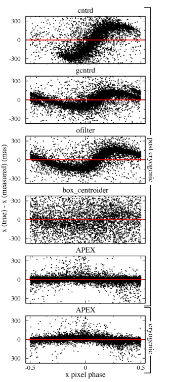
Figure 1.— The differences between true and measured x positions of stars in [3.6] images as a function distances of the measured position from the center of the pixel in the x direction for five routines: first derivative optimization (cntrd), Gaussian fitting (gcntrd), triangular weighting (ofilter), first moment (box_centroider), and PRF fitting (APEX). The first four routines produce large systematic errors ($>$ 100 mas) while APEX exhibits much smaller offsets in both the cryogenic and post-cryogenic data. Similar results are produced for y in [3.6] and x an y in [4.5]. Only detections with S/N $>$ 20 are plotted.

Figure 2.— Comparison of [3.6] x positional errors between APEX (blue) and four other methods for measuring positions (red) as a function of S/N. The solid lines are the median errors and the shaded regions encompass 80% of the errors. APEX produces the most precise positions at all values of S/N.

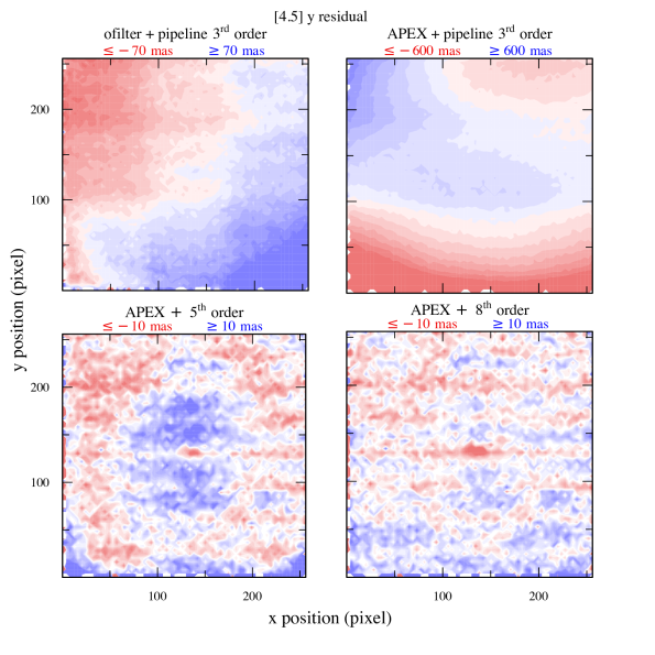
Figure 3.— Deviations from true y positions of sources in [4.5] images for different combinations of algorithms for measuring pixel coordinates and distortion corrections. The correction in the top panels is from the Spitzer data pipeline while those in the bottom panels have been derived in this work. In the top panels, we find that the ofilter routine produces much smaller residuals than APEX for the pipeline distortion correction. The bottom panels demonstrate that higher order distortion corrections can produce more accurate astrometry than the 3^rd order pipeline correction.

Figure 4.— Deviations from true x and y positions of sources in [3.6] and [4.5] images of Taurus produced by our final 7^th and 8^th order corrections, which were derived from data in the Galactic plane. We mark bad pixels (within solid rectangles) and pixels near the edges of the arrays (outside of dotted lines) where APEX produces erroneous positions, which were omitted from the derivation of our distortion corrections.

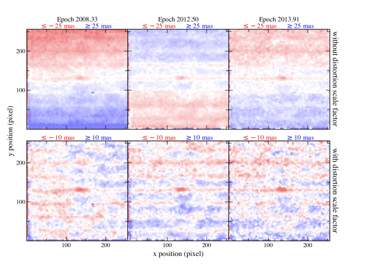
Figure 5.— Deviations from true y positions of sources in [4.5] images for one cryogenic epoch (2008.33) and two post cryogenic epochs (2012.50 and 2013.91). The residual maps in the top panel are produced with our distortion correction derived from data in the Galactic Plane (2011.58). The systematic offsets in each of those maps can be fit by a scale factor applied to the distortion correction. After applying such scale factors, we arrive at the residual maps in the bottom panel. The scale factors that we derive from these maps and datasets at additional epochs are shown in Figure 6.

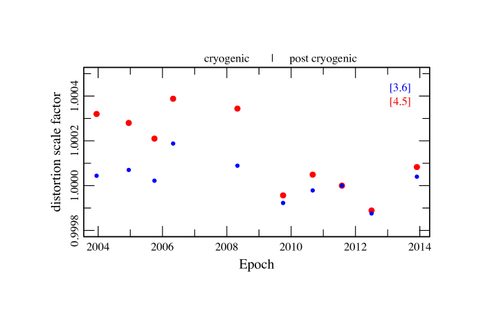
Figure 6.— Scale factors applied to our distortion corrections for [3.6] and [4.5] for datasets from various epochs during the Spitzer mission. The application of these factors removes the systematic offsets in residual maps like those shown in Figure 5.

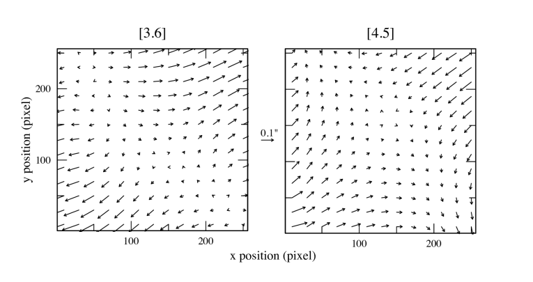
Figure 7.— Deviations of the distortions implied by our 7^th and 8^th corrections from a uniform plate scale for [3.6] and [4.5]. The deviations have been magnified by a factor of 200.

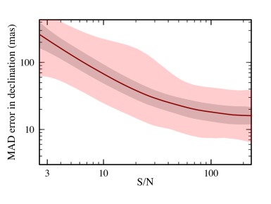
Figure 8.— Errors in declination for sources in IRAC images of the Chamaeleon I star-forming region as a function of S/N after applying our adopted distortion corrections (grey points). The median errors are plotted as the sold line and the darker and lighter shaded regions encompasses 50% and 90% of the errors, respectively. At S/N $>$ 100, the errors are less than 20 mas for half of the sources, which is the expected value if the error was due almost entirely to the measured positions (see Fig. 2) rather than errors in the distortion corrections or the relative positions and orientations among the dithered images.

References

- Beichman et al. (2013) Beichman, C., Gelino, C. R., Kirkpatrick, J. D., et al. 2013, ApJ, 764, 101
- Beichman et al. (2014) Beichman, C., Gelino, C. R., Kirkpatrick, J. D., et al. 2014, ApJ, 783, 68
- Calabretta & Greisen (2002) Calabretta, M. R., & Greisen, E. W. 2002, A&A 395, 1077
- Dupuy & Kraus (2013) Dupuy, T. J., & Kraus, A. L. 2013, Science, 341, 1492
- Fazio et al. (2004) Fazio, G. G., Hora, J. L., Allen, L. E., et al. 2004, ApJS, 154, 10
- Ingalls et al. (2012) Ingalls, J. G., Krick, J. E., Carey, S. J., et al. 2012, SPIE, 8442, 1
- Kirkpatrick et al. (2013) Kirkpatrick, J. D., Cushing, M. C., Gelino, C. R., et al. 2013, ApJ, 776, 128
- Kirkpatrick et al. (2014) Kirkpatrick, J. D., Schneider, A., Fajardo-Acosta, S., et al. 2014, ApJ, 783, 122
- Krick et al. (2015) Krick, K., Ingalls, J., Carey, S., et al. 2015, IRAC High Precision Photometry Website, http://irachpp.spitzer.caltech.edu
- Lewis et al. (2013) Lewis, N. K., Knutson, H. A., Showman, A. P., et al. 2013, ApJ, 766, 95
- Lowrance et al. (2014) Lowrance, P. J., Carey, S. J., Ingalls, J. G., et al. 2014, SPIE, 9143, 58
- Luhman (2014) Luhman, K. L. 2014, ApJL, 786, L18
- Luhman & Esplin (2014) Luhman, K. L., & Esplin, T. L. 2014, ApJ, 796, 6
- Makovoz & Marleau (2005) Makovoz, D., & Marleau, F. R. 2005, PASP, 117, 1113
- Marsh et al. (2013) Marsh, K. A., Wright, E. L., Kirkpatrick, J. D., et al. 2013, ApJ, 762, 119
- Metchev et al. (2015) Metchev, S. A., Heinze, A., Apai, D., et al. 2015, ApJ, 799, 154
- Mighell (2008) Mighell, K. J. 2008, SPIE, 7019, 1
- R Core Team (2013) R Core Team, 2013, R Foundation for Statistical Computing, Vienna, Austria, http://www.R-project.org
- Schwarz (1978) Schwarz, G. E. 1978, Annals of Statistics, 6, 461
- Shupe et al. (2005) Shupe, D. L., Moshir, M., Li, J., et al. 2005, ASPC, 347, 491
- Skrutskie et al. (2006) Skrutskie, M., Cutri, R. M., Stiening, R., et al. 2006, AJ, 131, 1163
- Thompson et al. (2013) Thompson, M. A., Kirkpatrick, J. D., Mace, G. N., et al. 2013, PASP, 125, 809
- Werner et al. (2004) Werner, M. W., Roellig, T. L., Low, F. J., et al. 2004, ApJS, 154, 1