Nonperturbative contribution to the strange-antistrange asymmetry of the nucleon sea

Abstract

We give predictions for the nonperturbative (intrinsic) contribution to the $s(x)-\bar{s}(x)$ asymmetry of the nucleon sea. For this purpose we use different light-front wave functions inspired by the AdS/QCD formalism, together with a model of the nucleon in terms of meson-baryon fluctuations. The holographic wave functions for an arbitrary number of constituents, recently derived by us, give results quite close to known parametrizations that appear in the literature.

I Introduction

Nowadays it is confirmed that hadrons are built by valence quarks together with a sea of $q\bar{q}$ pairs and gluons. This sea plays an important role in the understanding of several hadronic properties and provides an explanation of many experimental results in hadronic physics (for overviews and discussions of experimental and theoretical progress in this field see e.g. Refs. Sullivan:1971kd -Feng:2012gu ). In this vein one of the interesting aspects is the study of the strange quark sea and the $s(x)-\bar{s}(x)$ asymmetry, since both experimental and theoretical analyses indicate the existence of an strange-quark asymmetry (SQA) in the nucleon sea. Therefore, this asymmetry is a major hadronic observable, whose study can shed light on our understanding of the nucleon structure.

There are two main mechanisms that can generate a SQA in the nucleon sea – nonperturbative (intrinsic) and perturbative (extrinsic) (see e.g. discussion in Refs. Catani:2004nc ; Feng:2012gu ). The nonperturbative (or intrinsic) contribution to the strange-quark asymmetry can be considered to originate from nucleons fluctuating into virtual baryon-meson states ($\Lambda K$ and $\Sigma K$). These contributions can be estimated by using nonperturbative models for the nucleons Signal:1987gz ; Brodsky:1996hc ; Cao:1999da and are shown to be dominant in the large-$x$ region. As was shown in Ref. Catani:2004nc , the perturbative SQA, which is significant in the small-$x$ region, is produced by perturbative QCD evolution at next-to-next-to-leading order (NNLO) or at three loops. Such phenomenon occurs even if the SQA vanishes at the initial scale due to nonvanishing $u$ and $d$ valence quark densities Catani:2004nc .

In this work we give predictions for the nonperturbative contribution to the $s(x)-\bar{s}(x)$ asymmetry, following the light-front approach proposed by Brodsky and Ma Brodsky:1996hc . This approach deals with two-body light-front wave functions (LFWF) describing meson-baryon fluctuations of the proton in convolution with specific quark LFWFs. The result was that $s(x)<\bar{s}(x)$ at small-$x$ and $s(x)>\bar{s}(x)$ at large-$x$, which is a behavior opposite to the one obtained in meson cloud models Cao:1999da . In Ref. Brodsky:1996hc both Gaussian and power-law quark LFWFs were considered, leading to similar results. We intend to clarify this issue, using what we consider are more realistic LFWFs. For this purpose we use three different kinds of wave functions and show that the asymmetry is quite sensitive to the LFWFs. Therefore, the study of the $s-\bar{s}$ asymmetry could serve as a further tool to distinguish between these LFWFs. In particular, we consider the traditional Gaussian wave function Brodsky:1996hc and two variants of LFWFs motivated by AdS/QCD models. These last ones are extracted by matching electromagnetic form factors in LF QCD and AdS/QCD for the massless case, and introducing modifications in order to take into account finite quark masses Brodsky:2006uqa . Notice that the same matching procedure allows for an extraction of GPDs Vega:2010ns and, in addition, for a generalization of the LFWFs for hadrons with an arbitrary number of constituents Gutsche:2013zia . In particular, we consider an holographic LFWF (variant I) obtained from matching to LF QCD at large $x$ and a holographic LFWF (variant II) obtained from matching to LF QCD at all values of $x$ and for an arbitrary number of constituents Gutsche:2013zia . The second type of holographic LFWF is more useful for our purposes, because it can be applied to the description of hadrons with an arbitrary number of constituents.

We should stress that the all three LFWFs can reproduce hadronic experimental data (e.g see Brodsky:2006uqa ; Liu:2015jna ), and therefore the study of the s-sbar asymmetry serves as an independent tool to asses which of these functions provides a better phenomenological description of the nucleon. All considered LFWFs contain the scale parameter $\kappa$, which has been fixed at the value that gives the best description of the data. For completeness we also consider the sensitivity of the $s(x)-\bar{s}(x)$ asymmetry to a choice of this parameter.

The paper is structured as follows. In Sec. II we introduce the main ingredients of the light-front approach that we use to calculate the $s(x)-\bar{s}(x)$ asymmetry. Then we briefly describe the set of LFWFs used in our calculations. In Sec. III we discuss our results. Finally in Sec. IV we present our conclusions.

II $s(x)-\bar{s}(x)$ asymmetry in a light cone approach

In the light-front formalism the proton state can be expanded in a series of components as

$$|P\rangle = |uud\rangle\psi_{uud/p}+|uudg\rangle\psi_{uudg/p}$$ (1)

$$+ \sum_{q\bar{q}}|uudq\bar{q}\rangle\psi_{uudq\bar{q}/p}+\ldots$$

where $|uud\rangle$, $|uudg\rangle$, $|uudq\bar{q}\rangle$, $\ldots$ are the contributing Fock states and $\psi_{uud/p}$, $\psi_{uudg/p}$, $\psi_{uudq\bar{q}/p}$, $\ldots$ are the quark/gluon LFWFs corresponding to these states. In Ref. Brodsky:1996hc a different light front approach was proposed, in which the nucleon has components arising from meson-baryon fluctuations, while these hadronic components are composite systems of quarks. This approach is similar to expansions used in meson-cloud models Sullivan:1971kd . In this case the nonperturbative contributions to the $s(x)$ and $\bar{s}(x)$ distributions in the proton can be expressed as convolutions (see e.g. Ref. Cao:1999da )

$$s(x)=\int_{x}^{1}\frac{dy}{y}f_{\Lambda/K\Lambda}(y)q_{s/\Lambda}\biggl{(}\frac{x}{y}\biggl{)}\,,$$ (2)

$$\bar{s}(x)=\int_{x}^{1}\frac{dy}{y}f_{K/K\Lambda}(y)q_{\bar{s}/K}\biggl{(}\frac{x}{y}\biggl{)}\,,$$ (3)

where $q_{s/\Lambda}$ and $q_{\bar{s}/K}$ are distributions of $s$ quarks and $\bar{s}$ antiquarks in the $\Lambda^{0}(\Sigma^{0})$ and $K^{+}$, respectively. The functions $f_{\Lambda/K\Lambda}(y)$ and $f_{K/K\Lambda}(y)$ describe the probability to find a $\Lambda$ or a $K$ with light-front momentum fraction y in the $K\Lambda$ state.

In the light-front model proposed in Brodsky:1996hc the meson-baryon distribution functions are calculated through the relation

$$f_{B/BM}(y)=\int\frac{d^{2}{\bf k}_{\perp}}{16\pi^{3}}|\psi_{BM}(y,{\bf k}_{\perp})|^{2}.$$ (4)

where $\psi_{BM}(y,{\bf k}_{\perp})$ is the LFWF describing the distribution of the baryon-meson (BM) components. An important property of these functions, which follows from momentum and charge conservation, is that $f_{BK}(y)=f_{KB}(1-y)$ Holtmann:1996be . Here we have defined $f_{BK}(y)=f_{B/BK}(y)$ and $f_{KB}(y)=f_{K/BK}(y)$. In this work we consider a fluctuation probability for $N\rightarrow\Lambda K$ of $1.27\%$, as in Ref. Cao:1999da .

In the same manner, the distribution functions $q_{s/\Lambda}$ and $q_{\bar{s}/K}$ can be determined by

$$q_{s/\Lambda}(x) = \int\frac{d^{2}{\bf k}_{\perp}}{16\pi^{3}}|\psi_{\Lambda}(x,{\bf k}_{\perp})|^{2}\,,$$ (5)

$$q_{\bar{s}/K}(x) = \int\frac{d^{2}{\bf k}_{\perp}}{16\pi^{3}}|\psi_{K}(x,{\bf k}_{\perp})|^{2}\,.$$ (6)

To calculate $f_{\Lambda/K\Lambda}$, $f_{K/K\Lambda}$, $q_{s/\Lambda}$ and $q_{\bar{s}/K}$ it is necessary to know the LFWF for the distribution of $\Lambda$ and $K$ inside the states $\Lambda K$ and $\Sigma K$, and for the quarks/antiquarks in the $\Lambda$ and $K$. As we mentioned before, in this paper we use three different kinds of the LFWFs: i) a typical Gaussian LFWF Brodsky:1996hc , ii) a so-called holographic LFWFs obtained using light-front holography ideas Brodsky:2006uqa at large $x$ and iii) a further generalization which is extracted from matching at any value of $x$ and that further allows to describe hadrons with an arbitrary number of constituents Gutsche:2013zia . In the first two cases we directly follow the ideas of Ref. Brodsky:1996hc , where two-body wave functions $\psi_{BM}$ are formed by two clusters - baryon (as a quark-diquark bound state) and meson (as the usual quark-antiquark bound state). The third LFWF considers hadrons with an arbitrary number of constituents in the two-body approximation. In particular, the twist-5 wave function corresponds to the LFWF of the baryon-meson bound state $\psi_{BM}$. For the inclusion of massive constituents (baryon and meson) we follow the procedure proposed and realized in Refs. Brodsky:2006uqa . In the next subsections we give details of all LFWF used in our calculations.

II.1 Gaussian wave function

Brodsky and Ma Brodsky:1996hc suggested to use two-body Gaussian and power-law wave functions to calculate the $s(x)$ and $\bar{s}(x)$ asymmetry. They got similar results in both cases. Here we first consider the Gaussian wave function specified as

$$\psi(x,{\bf k}_{\perp})=A\exp\biggl{[}-\frac{1}{8\kappa^{2}}\biggl{(}\frac{{\bf k}_{\perp}^{2}}{x(1-x)}+\mu_{12}^{2}\biggr{)}\biggr{]}\,,$$ (7)

where

$$\mu_{12}^{2}=\frac{m_{1}^{2}}{x}+\frac{m_{2}^{2}}{1-x}$$ (8)

and $m_{1}$ and $m_{2}$ are the masses of the constituents.

In this approach, the functions $f_{\Lambda/K\Lambda}$ and $f_{K/K\Lambda}$ are calculated as

$$f_{\Lambda/K\Lambda}(x) = \frac{\kappa^{2}A_{MB}^{2}}{4\pi^{2}}\,x(1-x)\,\exp\biggl{[}-\frac{\mu_{\Lambda K}^{2}}{4\kappa^{2}}\biggr{]}\,,$$ (9)

$$f_{K/K\Lambda}(x) = \frac{\kappa^{2}A_{MB}^{2}}{4\pi^{2}}\,x(1-x)\,\exp\biggl{[}-\frac{\mu_{K\Lambda}^{2}}{4\kappa^{2}}\biggr{]}\,.$$ (10)

These LFWFs satisfy the constraint $f_{BK}(x)=f_{KB}(1-x)$. On the other side, the distribution functions $q_{s/\Lambda}$ and $q_{\bar{s}/K}$ are given by

$$q_{s/\Lambda}(x) = \frac{\kappa^{2}A_{B}^{2}}{4\pi^{2}}\,x(1-x)\,\exp\biggl{[}-\frac{\mu_{sD}^{2}}{4\alpha^{2}}\biggr{]}\,,$$ (11)

$$q_{\bar{s}/K}(x) = \frac{\kappa^{2}A_{M}^{2}}{4\pi^{2}}\,x(1-x)\,\exp\biggl{[}-\frac{\mu_{\bar{s}K}^{2}}{4\kappa^{2}}\biggr{]}\,.$$ (12)

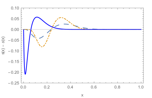
Figure 1: $s(x)-\bar{s}(x)$ plots for three different types of LFWFs: Gaussian LFWF (large dashed line – $\kappa=330$ MeV), holographic LFWF (variant I), (dot dashed line – $\kappa=350$ MeV) and holographic LFWF (variant II)(continuous line – $\kappa=350$ MeV).

Note that all the parameters involved in our calculations — constituent masses of quarks $m_{q}=330$ MeV, $m_{s}=480$ MeV, of diquark $m_{D}=600$ MeV, characteristic internal scale $\kappa=330$ MeV — have been fixed in Ref. Brodsky:1996hc and we use exactly the same set of parameters. The masses of hadrons involved in the calculation are $m_{\Lambda}=1115.683$ MeV and $m_{K^{+}}=493.677$ MeV. The normalization constants $A_{MB}$, $A_{B}$ and $A_{M}$ are obtained considering that the meson-baryon ($f_{\Lambda/K\Lambda}$, $f_{K/K\Lambda}$) and quark distribution ($q_{s/\Lambda}$, $q_{\bar{s}/K}$) functions are normalized to one:

$$\int\limits_{0}^{1}\!dxf_{K(\Lambda)/K\Lambda}(x)\!=\!\int\limits_{0}^{1}\!dxq_{s/\Lambda}(x)\!=\!\int\limits_{0}^{1}\!dxq_{\bar{s}/K}(x)\!=\!1\,.$$ (13)

Actually, these normalizations are correct when we do not include the probability for a meson-baryon fluctuation. When this probability is included, which is actually the case for equations (2) and (3), then the meson-baryon distribution normalizations should contain this probability. As mentioned before, here we have taken the fluctuation probability for $N\rightarrow\Lambda K$ to be $1.27\%$.

II.2 Holographic wave functions

In this section we consider two-body wave functions obtained by using light-front holography Brodsky:2006uqa . Specifically we use two types of wave functions – variant I (obtained from matching to LF QCD at large $x$) and variant II (obtained from matching at all values of $x$ and for an arbitrary number of constituents)

$$\psi(x,{\bf k}_{\perp}) = \frac{A}{\sqrt{x(1-x)}}$$ (14)

$$\times \exp\biggl{[}-\frac{1}{2\kappa^{2}}\biggl{(}\frac{{\bf k}_{\perp}^{2}}{x(1-x)}+\mu_{12}^{2}\biggr{)}\biggr{]}$$

and

$$\psi_{\tau}(x,{\bf k}_{\perp}) = A_{\tau}f_{\tau}(x)$$ (15)

$$\times \exp\biggl{[}-\frac{x\log(1/x)}{2\kappa^{2}(1-x)}\biggl{(}\frac{{\bf k}_{\perp}^{2}}{x(1-x)}+\mu_{12}^{2}\biggr{)}\biggr{]}\,,$$

where

$$f_{\tau}(x)=\frac{4\pi}{\kappa}\sqrt{\log(1/x)}(1-x)^{\frac{\tau-4}{2}}\,.$$ (16)

Here $\tau$ is the twist of the operator that creates these states, which in this case coincides with the number of constituents of the particular state.

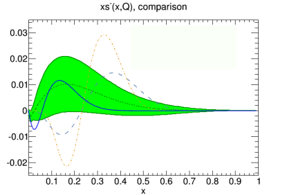
Figure 2: $xS^{-}=x(s(x)-\bar{s}(x))$. Green region and small dashed line correspond to MMHTHarland-Lang:2014zoa ) that it was generated with APFEL Carrazza:2014gfa . Other lines correspond to same cases in Fig. 1.

The first function satisfies the constraint $f_{BM}(x)=f_{MB}(1-x)$ with masses which are the same as used in the Gaussian case. The second LFWF Gutsche:2013zia is also a two-body wave function, describing both clusters as quark-diquark bound states. For both holographic LFWFs we take the same value $\kappa=350$ MeV fixed previoously from the best description of data on hadron properties Gutsche:2013zia .

In our specific calculations of the meson-baryon distribution functions we use $\tau=5$ with masses $m_{1}=m_{B}$ and $m_{2}=m_{M}$. Note that the condition $f_{BM}(x)=f_{MB}(1-x)$ is not satisfied in the case of the second holographic LFWF. To avoid this problem we define the meson-baryon distribution functions as

$$f_{BM}(x) = \int\frac{d^{2}{\bf k}_{\perp}}{16\pi^{3}}|\phi_{BM}(x,{\bf k}_{\perp})|^{2}\,,$$

$$\phi_{BM}(x,{\bf k}_{\perp}) = \psi_{5}(x,{\bf k}_{\perp})+\psi_{5}(1-x,{\bf k}_{\perp})\,.$$ (17)

To calculate $q_{s/\Lambda}$ and $q_{\bar{s}/K}$ we directly use equation (15) with $\tau=3$ and $2$ respectively. The parameters used in this case are the same as in the case of the holographic LFWF (variant II), also normalized to one.

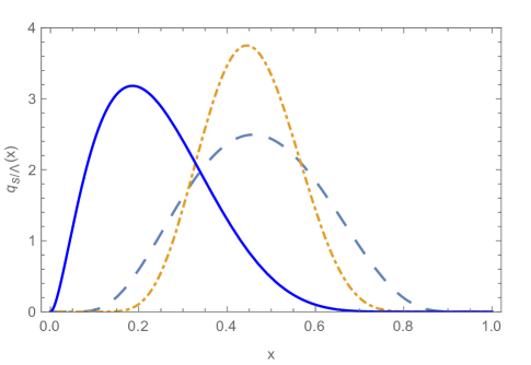
Figure 3: Strange quark density $q_{s/\Lambda}$. All notations as in Fig. 1.

III Results

Table 1: Second moment $\langle x(s-\bar{s})\rangle$

$\kappa$ (MeV)	Gaussian LFWF
330	0.00134
500	0.00108
1000	0.00058
$\kappa$ (MeV)	Holographic LFWF (I)
350	0.00157
550	0.00150
700	0.00143
$\kappa$ (MeV)	Holographic LFWF (II)
350	0.00091
550	0.00065
700	0.00047

For each LFWF we have calculated the meson-baryon distribution functions $f_{\Lambda/K\Lambda}$, $f_{K/K\Lambda}$ and the quark distributions $q_{s/\Lambda}$ and $q_{\bar{s}/K}$. Then using these quantities we calculate $s(x)-\bar{s}(x)$. Fig. I shows results for all three types of LFWFs using two slightly different values for the scale parameter $\kappa$, for reasons explained before. Notice that in both the Gaussian and the first holographic case (variant I) the point where the asymmetry vanishes is at $x\sim 0.7$, whereas in the other holographic case (variant II) it is near $x\sim 0.35$. Fig. 2 shows results for $x(s(x)-\bar{s}(x))$ calculated with models discussed here. Considering the value and location of maximum in $x(s(x)-\bar{s}(x))$, and region where start to be zero, we can see that our result for the holographic LFWF (variant II) is consistent with the result of the fit done in MMHT Harland-Lang:2014zoa .

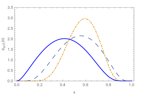
Figure 4: Strange quark density $q_{\bar{s}/K^{+}}$. All notations as in Fig. 1.

Figs. 3 and 4 show our predictions for the $s$- ($q_{s/\Lambda}$) and $\bar{s}$-quark ($q_{\bar{s}/K^{+}}$) distributions for the three variants of the LFWF. By inspection of Figs. 2 and 3 we can conclude that the results for the Gaussian and holographic (variant I) LFWF are close to each other, while the results for the holographic LFWF (variant II) are different. For the holographic LFWF (variant II) we get consistency with the results of the global fit performed by MMHTHarland-Lang:2014zoa .

Finally in Table I we present the results for the second moment $\langle x(s-\bar{s})\rangle$, using the different LFWFs. This quantity is defined as

$$\langle x(s-\bar{s})\rangle=\int\limits_{0}^{1}dxx\Big{(}s(x)-\bar{s}(x)\Big{)}\,,$$ (18)

where the $s(x)$ and $\bar{s}(x)$ are defined in Eqs. 2 and  3. All our results for the second moment are small, positive and consistent with a value $\langle x(s-\bar{s})\rangle\approx 0.005$ mentioned in Ref. Catani:2004nc , which would be required to attribute the NuTeV anomaly Zeller:2001hh to the strange asymmetry alone. The value is also in a good agreement with predictions of different models of $|\langle x(s-\bar{s})\rangle|\sim 10^{-4}$ (see discussion in Ref. Catani:2004nc ). For completeness, we also quote some other results for the second moment generated in nonperturbative mechanisms. The result $\langle x(s-\bar{s})\rangle=-0.0027\pm 0.0013$ Zeller:2002du was deduced from a lowest-order QCD analysis of neutrino data, $-0.001<\langle x(s-\bar{s})\rangle<0.004$ from a global QCD fit done in Ref. Olness:2003wz . Finally we mention the result for the second moment generated in a perturbative mechanism in Ref. Catani:2004nc of $\langle x(s-\bar{s})\rangle\approx-5\times 10^{-4}$ at the scale $Q^{2}=20$ GeV². Last result does not change too much when evolved to low scales and lies in the band derived in Ref. Olness:2003wz .

IV Conclusions

We calculated the $s(x)-\bar{s}(x)$ asymmetry in a light-front model considering three types of LFWFs. In all of these cases we observe that $s(x)<\bar{s}(x)$ for small values of $x$ and $s(x)>\bar{s}(x)$ in the region of large $x$. This behavior is exactly opposite to the one obtained in meson-cloud models. For the cases of the Gaussian and the holographic (variant I) LFWFs the asymmetry vanishes at $x\sim 0.6$, while for the second variant of the holographic LFWF this point moves to a lower value of $x\sim 0.35$. The latter case is closer to MMHT Harland-Lang:2014zoa (other recent parametrizations are NNPDF Ball:2014uwa , MSTW Martin:2009iq , MMHT Harland-Lang:2014zoa and nCTEQ Kusina:2015vfa ). Finally, our predictions for the second moment of the strange quark asymmetry $\langle x(s-\bar{s})\rangle=0.00102\pm 0.00055$ are consistent with previous results obtained with nonperturbative mechanisms.

Holographic wave functions has been used to calculate hadron properties, and his parameters was fixed, therefore, the study of the s-sbar asymmetry serves as independent tool to distinguish these functions. We present the results for fixed value of the $\kappa$, although for completeness also allow a variation of this parameter to display the sensitivity of s-sbar asymmetry to a choice of this parameter.

- (1) J. D. Sullivan, Phys. Rev. D 5, 1732 (1972); A. W. Thomas, Phys. Lett. B 126, 97 (1983); M. Burkardt and B. Warr, Phys. Rev. D 45, 958 (1992); C. Boros, J. T. Londergan and A. W. Thomas, Phys. Rev. Lett. 81, 4075 (1998); M. Burkardt, C. A. Miller and W. D. Nowak, Rept. Prog. Phys. 73, 016201 (2010).
- (2) A. I. Signal and A. W. Thomas, Phys. Lett. B 191, 205 (1987); H. R. Christiansen and J. Magnin, Phys. Lett. B 445, 8 (1998).
- (3) H. Holtmann, A. Szczurek and J. Speth, Nucl. Phys. A 596, 631 (1996); W. Melnitchouk, J. Speth and A. W. Thomas, Phys. Rev. D 59, 014033 (1998).
- (4) S. A. Rabinowitz et al., Phys. Rev. Lett. 70, 134 (1993); A. O. Bazarko et al. (CCFR Collaboration), Z. Phys. C 65, 189 (1995); M. Arneodo et al. (New Muon Collaboration), Nucl. Phys. B 483, 3 (1997); W. G. Seligman et al., Phys. Rev. Lett. 79, 1213 (1997).
- (5) S. J. Brodsky and B. Q. Ma, Phys. Lett. B 381, 317 (1996).
- (6) M. Gluck, E. Reya and M. Stratmann, Eur. Phys. J. C 2, 159 (1998); M. Gluck, E. Reya and A. Vogt, Eur. Phys. J. C 5, 461 (1998); M. Gluck, E. Reya, M. Stratmann and W. Vogelsang, Phys. Rev. D 63, 094005 (2001).
- (7) A. D. Martin, R. G. Roberts, W. J. Stirling and R. S. Thorne, Eur. Phys. J. C 14, 133 (2000); H. L. Lai et al. (CTEQ Collaboration), Eur. Phys. J. C 12, 375 (2000); S. I. Alekhin, Phys. Rev. D 63, 094022 (2001); A. Kusina et al., Phys. Rev. D 85, 094028 (2012).
- (8) F. G. Cao and A. I. Signal, Phys. Rev. D 60, 074021 (1999).
- (9) F. Olness et al., Eur. Phys. J. C 40, 145 (2005).
- (10) R. D. Ball et al. [NNPDF Collaboration], JHEP 1504, 040 (2015).
- (11) A. D. Martin, W. J. Stirling, R. S. Thorne and G. Watt, Eur. Phys. J. C 63, 189 (2009) doi:10.1140/epjc/s10052-009-1072-5 [arXiv:0901.0002 [hep-ph]].
- (12) L. A. Harland-Lang, A. D. Martin, P. Motylinski and R. S. Thorne, Eur. Phys. J. C 75, no. 5, 204 (2015).
- (13) S. Catani, D. de Florian, G. Rodrigo and W. Vogelsang, Phys. Rev. Lett. 93, 152003 (2004).
- (14) M. Salajegheh, Phys. Rev. D 92, no. 7, 074033 (2015).
- (15) G. Q. Feng, F. G. Cao, X. H. Guo and A. I. Signal, Eur. Phys. J. C 72, 2250 (2012).
- (16) S. J. Brodsky and G. F. de Teramond, Phys. Rev. Lett. 96, 201601 (2006); Phys. Rev. D 77, 056007 (2008); S. J. Brodsky, G. F. de Teramond, H. G. Dosch and J. Erlich, Phys. Rept. 584, 1 (2015; A. Vega, I. Schmidt, T. Branz, T. Gutsche and V. E. Lyubovitskij, Phys. Rev. D 80, 055014 (2009); T. Branz, T. Gutsche, V. E. Lyubovitskij, I. Schmidt and A. Vega, Phys. Rev. D 82, 074022 (2010); T. Gutsche, V. E. Lyubovitskij, I. Schmidt and A. Vega, Phys. Rev. D 85, 076003 (2012).
- (17) A. Vega, I. Schmidt, T. Gutsche and V. E. Lyubovitskij, Phys. Rev. D 83, 036001 (2011); Phys. Rev. D 85, 096004 (2012).
- (18) T. Gutsche, V. E. Lyubovitskij, I. Schmidt and A. Vega, Phys. Rev. D 89, 054033 (2014).
- (19) T. Liu and B. Q. Ma, Phys. Rev. D 92, no. 9, 096003 (2015) doi:10.1103/PhysRevD.92.096003 [arXiv:1510.07783 [hep-ph]]. D. Chakrabarti, C. Mondal and A. Mukherjee, Phys. Rev. D 91, no. 11, 114026 (2015) T. Huang, B. Q. Ma and Q. X. Shen, Phys. Rev. D 49, 1490 (1994) B. W. Xiao, X. Qian and B. Q. Ma, Eur. Phys. J. A 15, 523 (2002) B. Q. Ma, D. Qing and I. Schmidt, Phys. Rev. C 65, 035205 (2002)
- (20) S. Carrazza, A. Ferrara, D. Palazzo and J. Rojo, J. Phys. G 42, no. 5, 057001 (2015)
- (21) T. Gutsche, V. E. Lyubovitskij, I. Schmidt and A. Vega, Phys. Rev. D 91, 054028 (2015); Phys. Rev. D 87, 056001 (2013).
- (22) G. P. Zeller et al. [NuTeV Collaboration], Phys. Rev. Lett. 88, 091802 (2002) [Phys. Rev. Lett. 90, 239902 (2003)].
- (23) G. P. Zeller et al. [NuTeV Collaboration], Phys. Rev. D 65, 111103 (2002) [Phys. Rev. D 67, 119902 (2003)].
- (24) A. Kusina et al., arXiv:1509.01801 [hep-ph].