Modular Bond-graph Modelling and Analysis
of Biomolecular Systems

Abstract

Bond graphs can be used to build thermodynamically-compliant hierarchical models of biomolecular systems. As bond graphs have been widely used to model, analyse and synthesise engineering systems, this paper suggests that they can play the same rôle in the modelling, analysis and synthesis of biomolecular systems. The particular structure of bond graphs arising from biomolecular systems is established and used to elucidate the relation between thermodynamically closed and open systems. Block diagram representations of the dynamics implied by these bond graphs are used to reveal implicit feedback structures and are linearised to allow the application of control-theoretical methods.

Two concepts of modularity are examined: computational modularity where physical correctness is retained and behavioural modularity where module behaviour (such as ultrasensitivity) is retained. As well as providing computational modularity, bond graphs provide a natural formulation of behavioural modularity and reveal the sources of retroactivity. A bond graph approach to reducing retroactivity, and thus inter-module interaction, is shown to require a power supply such as that provided by the $ATP{\;\xrightleftharpoons{}\;}ADP+Pi$ reaction.

The MAPK cascade (Raf-MEK-ERK pathway) is used as an illustrative example.

1 Introduction

In their review paper The rôle of control and system theory in systems biology, Wellstead et al. [1] suggest that “systems biology is an area where systematic methods for model development and analysis, such as bond graphs, could make useful new contributions as they have done in the physical world”. The purpose of this paper is to show that bond graphs not only provide a systematic methods for model development and analysis of biomolecular systems but also provide a bridge allowing application of control engineering methodology, in particular feedback concepts, to systems biology.

Bond graphs were introduced by Paynter [2] and their engineering application is described in number of text books [3, 4, 5, 6] and a tutorial for control engineers [7]. Bond graphs were first used to model chemical reaction networks by Oster et al. [8] and a detailed account is given by Oster et al. [9]. Subsequent to this, the bond graph approach to chemical reactions has been extended by Cellier [10], Thoma and Mocellin [11] and Greifeneder and Cellier [12]. More recently, the bond graph approach has been used to analyse biochemical cycles by Gawthrop and Crampin [13] and has been shown to provide a modular approach to building hierarchical biomolecular system models which are robustly thermodynamically compliant [14]; combining thermodynamically compliant modules gives a thermodynamically compliant system. In this paper we will call this concept computational modularity.

Computational modularity is a necessary condition for building physically correct computational models of biomolecular systems. However, computational modularity does not imply that module properties (such as ultrasensitivity) are retained when a module is incorporated into a larger system. In the context of engineering, modules often have buffer amplifiers at the interface so that they have unidirectional connections and may thus be represented and analysed on a block diagram or signal flow graph where the properties of each module are retained. This will be called behavioural modularity in this paper. However, biological networks do not usually have this unidirectional property but rather display retroactivity [15, 16, 17, 18, 19, 20]; retroactivity modifies the properties of the interacting modules. As will be shown, the property of retroactivity is naturally captured by bond graphs. In particular, a bond graph approach to reducing retroactivity, and thus inter-module interaction, is discussed and shown to require a power supply such as that provided by the $ATP{\;\xrightleftharpoons{}\;}ADP+Pi$ reaction.

Early attempts at modelling the MAPK cascade [21, 22], used modules which displayed behavioural modularity. However, because they use the Michaelis-Menten approximation, the modules do not have the property of computational modularity and thus the results were based on a non-physical model. This was noted in later work which examined the neglected interactions: in particular, Ortega et al. [23] show that “product dependence and bifunctionality compromise the ultrasensitivity of signal transduction cascades” and the “effects of sequestration on signal transduction cascades” are considered by Bluthgen et al. [24]. In this paper, the MAPK cascade is used as an illustrative example which illustrates how a computationally modular approach based on bond graphs avoids the errors associated with assuming irreversible Michaelis-Menten kinetics. Moreover, the bond graph approach to reducing retroactivity is used to make the modules approximately modular in the behavioural sense. This emphasises the necessity for a power supply to support signalling networks in biology as well as in engineering.

The bond graph approach gives the set of nonlinear ordinary differential equations describing the biomolecular system being modelled. Linearisation of non-linear systems is a standard technique in control engineering: as discussed by Goodwin et al. [25], “The incentive to try to approximate a nonlinear system by a linear model is that the science and art of linear control is vastly more complete and simpler than they are for the nonlinear case.”. Nevertheless, it is important to realise that conclusions drawn from linearisation can only be verified using the full nonlinear equations. In the context of bond graphs, linearisation (and the associated concept of sensitivity) has been treated by a number of authors [26, 27, 28]. This paper builds on this work to explicitly derive the bond graph corresponding to the linearised nonlinear system and thus provide a method to analyse behavioural modularity.

§ 2 briefly shows how biomolecular systems can be modelled using bond graphs. § 3 shows how thermodynamically closed systems can be converted to thermodynamically open systems using the twin notions of chemostats and flowstats. Linearisation is required to understand module behaviour, and this is developed in § 4. § 5 looks at modularity, retroactivity and feedback and § 6 illustrates the main results using the MAPK cascade example. § 7 concludes the paper and suggests future research directions.

2 Bond Graph Modelling of Biomolecular Systems

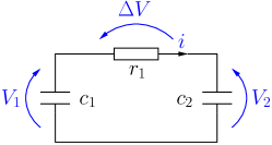
(a) Electrical Circuit

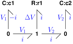
(b) Bond graph

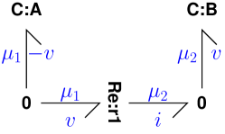
(c) Bond graph for $A{\;\xrightleftharpoons{1}\;}B$

Figure 1: Simple example. (a) An RC circuit schematic. (b) As discussed in the text, capacitors ($c_{1}$ & $c_{2}$) are represented by bond graph C components, resistors ($r_{1}$) by bond graph R components and connections by 0 and 1 junctions; the bonds ($\rightharpoondown$) carry the effort (voltage) and flow (current) variables. (c) The reaction $A{\;\xrightleftharpoons{1}\;}B$. As discussed in § 2.1, the 1 and R components are replaced by a single two port Re component representing the reaction and the C components correspond to the reactants $A$ and $B$.

As discussed by Maxwell [29], the use of “mathematical or formal analogy” enables us to avail “ourselves of the mathematical labours of those who had already solved problems essentially the same.” The bond graph approach provides a systematic approach to the use of analogy in the modelling of systems across different physical domains; in the context of this paper, this allows engineering concepts to be carried across to biomolecular systems.

A number of text books about bond graphs [3, 4, 5, 6] and a tutorial for control engineers [7] are available. Briefly, bond graphs focus on a pair of variables generically termed effort $e$ and flow $f$ whose product is power $p=ef$. In the electrical domain, effort is identified with voltage $V$ ($\mathrm{V}$) and flow with current $i$ ($\mathrm{C}\,\mathrm{s}\mathrm{e}\mathrm{c}^{-1}$) and in the mechanical domain effort is identified with force $F$ ($\mathrm{N}$) and flow with velocity $v$ ($\mathrm{m}\,\mathrm{s}\mathrm{e}\mathrm{c}^{-1}$). Thus voltage and force are effort analogies and current and velocity are flow analogies. Although the effort (and the flow) variables have different units in each domain, their product (power) has the same units ($\mathrm{W}$ or $\mathrm{J}\,\mathrm{s}\mathrm{e}\mathrm{c}^{-1}$); power is the common currency of disparate physical domains. The pair $e$ $f$ is represented on the bond graph by the harpoon symbol: $\rightharpoondown$ which can be optionally annotated with specific effort and flow variables, for example $\xrightharpoondown[f]{e}$. Sign convention is handled by the harpoon direction: thus if $e$ and $f$ are positive, the flow $f$ is in the harpoon direction.

As well as analogous variables, bond graphs deal in analogous components. Thus the bond graph C component models both the ideal electrical capacitor (with capacitance $c_{c}$) and the ideal mechanical spring (with stiffness $K_{s}$). In both cases, the C component physically accumulates flow to give the integrated flow $q$ corresponding to electrical charge or mechanical displacement. In the linear case, this gives an effort proportional to $q$. To summarise:

$$\dot{Q} =i V =\frac{Q}{c_{c}} (electrical)$$

$$\dot{x} =v F =K_{s}x (mechanical)$$

$$\dot{q} =f e =Kq (generic)$$ (1)

Similarly, electrical resistors and mechanical dampers are represented by bond graph R components where:

$$V =ri (electrical)$$ (2)

$$F =rv (mechanical)$$ (3)

$$e =rf (generic)$$ (4)

where $r$ represents the (linear) electrical resistance and mechanical damping factor.

Bonds are connected by 0 and 1 junctions which again conserve energy; the 0 junction gives the same effort on each impinging bond and the 1 junction gives the same flow on each impinging bond.

Figure 1 shows a simple electrical circuit connecting two capacitors with capacitance $c_{1}$ and $c_{2}$ by a resistor with resistance $r_{1}$. Figure 1(a) gives the electrical schematic diagram and Figure 1(b) gives the corresponding bond graph which uses the C , R , 0 and 1 components connected by bonds.

The bond graph TF component represents both an electrical transformer and a mechanical lever with ratio $\rho$. In generic terms, the bond graph fragment: $\xrightharpoondown[f_{1}]{e_{1}}$ TF:$\mathbf{\rho}$ $\xrightharpoondown[f_{2}]{e_{2}}$ represents the two equations:

$$f_{2} =\rho f_{1} e_{1} =\rho e_{2}$$ (5)

Note that energy is conserved as

$$p_{2}=e_{2}f_{2}=\frac{e_{1}}{\rho}\rho f_{1}=e_{1}f_{1}=p_{1}$$ (6)

2.1 Biomolecular bond graph components

It is assumed that biochemical reactions occur under conditions of constant pressure (isobaric) and constant temperature (isothermal). Under these conditions, the chemical potential $\mu_{A}$ of substance $A$ is given [30] in terms of its mole fraction $\chi_{A}$ as:

$$\mu_{A}=\mu_{A}^{\star}+RT\ln\chi_{A}~{}($~{}\mathrm{J}\,\mathrm{m}\mathrm{o}\mathrm{l}^{-1}$)$$ (7)

where the standard chemical potential $\mu_{A}^{\star}$ is the value of $\mu_{A}$ when $A$ is pure ($\chi_{A}=1$), $R=8.314~{}($~{}\mathrm{J}\mathrm{K}^{-1}\mathrm{m}\mathrm{o}\mathrm{l}^{-1}$)$ is the universal gas constant, $T~{}($\mathrm{K}$)$ is the absolute temperature and $\ln$ is the natural (or Napierian) logarithm. It is convenient to define a normalised chemical potential ${\check{\mu}}_{A}$ as:

$${\check{\mu}}_{A}=\frac{\mu_{A}}{RT}$$ (8)

The key to modelling chemical reactions by bond graphs is to determine the appropriate effort and flow variables. As discussed by Oster et al. [8, 9], the appropriate effort variable is chemical potential $\mu$ and the appropriate flow variable is molar flow rate $v$.

In the context of chemical reactions, the bond graph C component of Equation (1) is defined by Equation (7) as:

$$\dot{x}_{A} =v_{A}~{}($~{}\mathrm{m}\mathrm{o}\mathrm{l}\,\mathrm{s}\mathrm{e}\mathrm{c}^{-1}$) \mu_{A} =RT\ln K_{A}x_{A}~{}($~{}\mathrm{J}\,\mathrm{m}\mathrm{o}\mathrm{l}^{-1}$) (chemical)$$ (9)

where $x_{A}$ is the molar amount of $A$ and the thermodynamic constant $K_{A}$ is given by

$$K_{A}=\frac{1}{n_{total}}\exp{\frac{\mu_{A}^{\star}}{RT}}=\frac{1}{n_{total}}\exp{{\check{\mu}}_{A}^{\star}}~{}($~{}\mathrm{m}\mathrm{o}\mathrm{l}^{-1}$)$$ (10)

where $n_{total}$ is the total number of moles in the mixture. Alternatively, (9) can be written more simply in terms of the normalised chemical potential ${\check{\mu}}$ of Equation (8):

$$\dot{x}_{A} =v_{A}~{}($~{}\mathrm{m}\mathrm{o}\mathrm{l}\,\mathrm{s}\mathrm{e}\mathrm{c}^{-1}$) {\check{\mu}}_{A} =\ln K_{A}x_{A}$$ (11)

We follow Oster et al. [9] in describing chemical reactions in terms of the Marcelin – de Donder formulae as discussed by Van Rysselberghe [32] and Gawthrop and Crampin [13]. In particular, given the $i$th reaction [9, (5.9)]:

$$\nu^{f}_{A}A+\nu^{f}_{B}B+\nu^{f}_{C}C+\nu^{f}_{D}D\dots\;\xrightleftharpoons{i}\;\nu^{r}_{A}A+\nu^{r}_{B}B+\nu^{r}_{C}C+\nu^{r}_{D}D\dots$$ (12)

where the stoichiometric coefficients $\nu$ are either zero or positive integers, the forward affinity $A^{f}_{i}$ and the reverse affinity $A^{r}_{i}$ are defined as:

$$A^{f}_{i} =\nu^{f}_{A}\mu_{A}+\nu^{f}_{B}\mu_{B}+\nu^{f}_{C}\mu_{C}+\nu^{f}_{D}\mu_{D}\dots$$ (13)

$$A^{r}_{i} =\nu^{r}_{A}\mu_{A}+\nu^{r}_{B}\mu_{B}+\nu^{r}_{C}\mu_{C}+\nu^{r}_{D}\mu_{D}\dots$$ (14)

The units of affinity are the same as those of chemical potential: $\mathrm{J}\,\mathrm{m}\mathrm{o}\mathrm{l}^{-1}$. Again, normalised affinities are useful:

$${\check{A}}^{f}_{i} =\frac{A^{f}_{i}}{RT} {\check{A}}^{r}_{i} =\frac{A^{r}_{i}}{RT}$$ (15)

The $i$th reaction flow $v_{i}$ is then given by:

$$v_{i} =\kappa_{i}\left(v^{+}_{0}-v^{-}_{0}\right) \text{where }v^{+}_{0} =e^{\frac{A^{f}_{i}}{RT}}=e^{{\check{A}}^{f}_{i}} \text{and }v^{-}_{0} =e^{\frac{A^{r}_{i}}{RT}}\ =e^{{\check{A}}^{r}_{i}}$$ (16)

Note that the arguments of the exponential terms are dimensionless as are $v^{+}_{0}$ and $v^{-}_{0}$. The units of the reaction rate constant $\kappa_{i}$ are those of molar flow rate: $\mathrm{m}\mathrm{o}\mathrm{l}\,\mathrm{s}\mathrm{e}\mathrm{c}^{-1}$.

The $i$th reaction flow $v_{i}$ depends on the forward and reverse affinities $A^{f}_{i}$ and $A^{r}_{i}$ but cannot be written as the difference between the affinities. Unlike the electrical R component (see Figure 1), it cannot be written as a one port component with the flow dependent on the difference between the efforts. However, as discussed by Gawthrop and Crampin [13], a two port resistive component, the Re component, can be used to model the reaction (16).

The fact that the capacitive C and resistive Re components are intrinsically non-linear is one factor distinguishing biochemical systems from the electrical and mechanical systems of Equation (1).

The TF component is used in this context to account for any non-unity and non-zero stoichiometric coefficients $\nu$ in Equation (12) [8, 9, 13]. Moreover, as will be discussed in the next section, the TF component can be used to abstract the entire network of bonds, 0 and 1 junctions connecting the C and Re components.

2.2 Examples

Consider the simple reaction $A{\;\xrightleftharpoons{1}\;}B$. In this case ${\check{A}}^{f}={\check{\mu}}_{A}$ and ${\check{A}}^{r}={\check{\mu}}_{B}$. With reference to Figure 1(c), substance $A$ is modelled by C:$\mathbf{A}$, substance $B$ is modelled by C:$\mathbf{B}$ and the reaction by Re:$\mathbf{r1}$. The equations of the C components correspond to Equation (9) and that of the Re component to (16). The equations are:

$${\check{A}}^{f}={\check{\mu}}_{A} =\ln K_{A}x_{A} {\check{A}}^{r}={\check{\mu}}_{B} =\ln K_{B}x_{B}$$ (17)

$$v^{+}_{0} =e^{{\check{A}}^{f}}=K_{A}x_{A} v^{-}_{0} =e^{{\check{A}}^{r}}=K_{B}x_{B}$$ (18)

$$v =\kappa\left(K_{A}x_{A}-K_{B}x_{A}\right)=k^{+}x_{A}-k^{-}x_{B} \text{where }k^{+} =\kappa K_{A}\text{ and }k^{-}=\kappa K_{B}$$ (19)

In this simple case the equations are linear and the rate constants $k^{+}$ and $k^{-}$ are given in terms of the reaction rate-constant $\kappa$ and the thermodynamic constants $K_{A}$ and $K_{B}$. The equilibrium constant $K^{eq}$ is given by:

$$K^{eq}=\frac{k^{+}}{k^{-}}=\frac{K_{A}}{K_{B}}$$ (20)

and is thus a function of the thermodynamic constants $K_{A}$ and $K_{B}$ but not the reaction rate-constant $\kappa$. A general formula relating all the equilibrium constants in a biomolecular network to the rate constants is given by Gawthrop et al. [14, § 3].

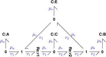
(a) Bond graph

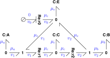
(b) Bond graph with enzyme degradation

Figure 2: Example: Enzyme catalysed reaction. (a) Bond graph of the enzyme catalysed reaction $A+E{\;\xrightleftharpoons{1}\;}C{\;\xrightleftharpoons{2}\;}B+E$. $A$ is the reactant, $B$ the product, $C$ the intermediate complex and $E$ the enzyme. ($A$ and $B$ are used as chemostats in § 3). (b) An enzyme degradation reaction Re:$\mathbf{r0}$ is added. (Re:$\mathbf{r0}$ is used as a flowstat in § 3).

The enzyme catalysed reaction

$$A+E{\;\xrightleftharpoons{1}\;}C{\;\xrightleftharpoons{2}\;}B+E$$ (21)

where $A$ is the reactant, $B$ the product, $C$ the intermediate complex and $E$ the enzyme, is ubiquitous in biochemical systems. The reaction (21) was first modelled using bond graphs by Oster et al. [9, Fig. 5.9].

Figure 2(a) is the bond graph corresponding to Equation (21). The components Re:$\mathbf{r1}$ and Re:$\mathbf{r2}$ represent reactions ${\;\xrightleftharpoons{1}\;}$ and ${\;\xrightleftharpoons{2}\;}$ and the four C components C:$\mathbf{A}$, C:$\mathbf{B}$, C:$\mathbf{C}$ and C:$\mathbf{E}$ represent the four species $A$, $B$, $C$ and $E$. The left-hand 1 junction ensures that the flow out of C:$\mathbf{A}$ and C:$\mathbf{E}$ is the reaction flow $v_{1}$ and the right-hand 1 junction ensures that the flow into C:$\mathbf{B}$ and C:$\mathbf{E}$ is the reaction flow $v_{2}$. The net flow into C:$\mathbf{E}$ is thus $v_{1}-v_{2}$.

The additional reaction Re:$\mathbf{r0}$ has been added in Figure 2(b) together with the zero-potential source $\boldsymbol{\oslash}$; this can be used to model enzyme degradation. C:$\mathbf{A}$ and C:$\mathbf{B}$ are used in § 3 as an example of a chemostat and Re:$\mathbf{r0}$ as an example of a flowstat. The enzyme catalysed reaction is analysed further in § 5.2.

3 Closed systems and open systems: chemostats and flowstats

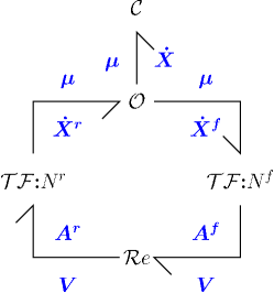
(a) Closed system bond graph

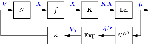
(b) Closed system block-diagram

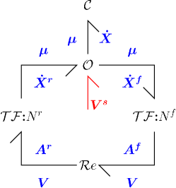
(c) Open system bond graph

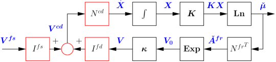
(d) Open system block diagram

Figure 3: Closed & open systems (a) General closed system. The bond symbols $\rightharpoondown$ correspond to vectors of bonds; $\mathcal{C}$, $\mathcal{R}e$ and $\mathcal{O}$ correspond to arrays of C , Re and 0 components ; the two $\mathcal{TF}$ components represent the intervening junction structure comprising bonds, 0 and 1 junctions and TF components. $N^{f}$ and $N^{r}$ are the forward and reverse stoichiometric matrices. (b) The corresponding block diagram. (d) The addition of the chemostat & flowstat flows $V^{s}$ to the closed system of Figure 3(a) gives an open system. (d) The corresponding block diagram.

Specific bond graphs (such as Figures 1(c) and 2(a)) model specific sets of chemical reactions. It is convenient to generalise such bond graphs to allow generic statements to be made and generic equations to be written. The molar amounts of the $n_{X}$ species $x_{A},x_{B},\dots$, the corresponding chemical potentials $\mu_{A},\mu_{B},\dots$ and the corresponding thermodynamic constants $K_{A},K_{B},\dots$ are collected into column vectors:

$$\boldsymbol{X} =\begin{pmatrix}x_{A}\\ x_{B}\\ \vdots\end{pmatrix} \boldsymbol{\mu} =\begin{pmatrix}\mu_{A}\\ \mu_{B}\\ \vdots\end{pmatrix} K =\begin{pmatrix}K_{A}\\ K_{B}\\ \vdots\end{pmatrix}$$ (22)

Similarly,the $n_{V}$ reaction flows $v_{1},v_{2},\dots$, affinities (forward and reverse) $A_{1},A_{2},\dots$ and the corresponding reaction constants $\kappa_{1},\kappa_{2},\dots$ are collected into column vectors:

$$\boldsymbol{V} =\begin{pmatrix}v_{1}\\ v_{2}\\ \vdots\end{pmatrix} \boldsymbol{A} =\begin{pmatrix}A_{1}\\ A_{2}\\ \vdots\end{pmatrix} \kappa =\begin{pmatrix}\kappa_{1}\\ \kappa_{2}\\ \vdots\end{pmatrix}$$ (23)

As discussed by Karnopp et al. [6], the C components can be subsumed into a single C -field, the Re components (as two-port R components) subsumed into an R-field and the connecting bonds, 0 and 1 junctions subsumed into a junction structure. Moreover, as this junction structure transmits, but does not store or dissipate energy, it can be modelled as the two multiport transformers $\mathcal{TF}{:}N^{f}$ and $\mathcal{TF}{:}N^{r}$ shown in Figure 3(a). These two multiport transformers are defined to transform flows as:

$$\dot{\boldsymbol{X}}^{r} =N^{r}\boldsymbol{V} \dot{\boldsymbol{X}}^{f} =N^{f}\boldsymbol{V}$$ (24)

Because they do not store or dissipate energy, it follows that the affinities are given by:

$$\boldsymbol{A}^{r} ={N^{r}}^{T}\boldsymbol{\mu} \boldsymbol{A}^{f} ={N^{f}}^{T}\boldsymbol{\mu}$$ (25)

As discussed by Gawthrop and Crampin [13], and with reference to Figure 3(a), the system states $\boldsymbol{X}$ correspond to the molar amounts of each species stored in each C components and are given in terms of the reaction flows $\boldsymbol{V}$ as

$$\dot{\boldsymbol{X}} =\dot{\boldsymbol{X}}^{r}-\dot{\boldsymbol{X}}^{f}=N\boldsymbol{V} \text{where }N =N^{r}-N^{f}$$ (26)

$N$ is the stoichiometric matrix [33]; $N^{f}$ and $N^{r}$ are referred to as the forward and reverse stoichiometric matrices.

From Equation (9), the composite chemical potential $\boldsymbol{\mu}$ is given by the non-linear equation:

$$\frac{\boldsymbol{\mu}}{RT} ={\boldsymbol{\check{\mu}}}=\text{\bf Ln }\boldsymbol{K}\boldsymbol{X} \text{where }\boldsymbol{K} =\text{diag }{K}$$ (27)

and from Equation (16), the composite reaction flow $\boldsymbol{V}$ is given by the non-linear equations

$$\boldsymbol{V}^{+}_{0} =\text{\bf Exp }\left(\frac{\boldsymbol{A}^{f}}{RT}\right)=\text{\bf Exp }{\boldsymbol{\check{A}}}^{f} \boldsymbol{V}^{-}_{0} =\text{\bf Exp }\left(\frac{\boldsymbol{A}^{r}}{RT}\right)=\text{\bf Exp }{\boldsymbol{\check{A}}}^{r}$$ (28)

$$\boldsymbol{V} =\boldsymbol{\kappa}\left(\boldsymbol{V}^{+}_{0}-\boldsymbol{V}^{-}_{0}\right) \text{where }\boldsymbol{\kappa} =\text{diag }{\kappa}$$ (29)

Defining the composite stoichiometric and composite reaction constant matrices $N^{fr}$ and $\boldsymbol{\kappa}^{fr}$ as.

$$N^{fr} =\begin{pmatrix}N^{f}&N^{r}\end{pmatrix} \text{and }\boldsymbol{\kappa}^{fr} =\begin{pmatrix}\boldsymbol{\kappa}&-\boldsymbol{\kappa}\end{pmatrix}$$ (30)

Equations (25), (28) and (29) can be rewritten in a more compact form as:

$${\boldsymbol{\check{A}}}^{fr} ={N^{fr}}^{T}{\boldsymbol{\check{\mu}}} \boldsymbol{V}_{0} =\text{\bf Exp }{\boldsymbol{\check{A}}}^{fr} \boldsymbol{V} =\boldsymbol{\kappa}^{fr}\boldsymbol{V}_{0}$$ (31)

which can be combined to give a compact expression for the flows $\boldsymbol{V}$ in terms of the state $\boldsymbol{X}$

$$\boldsymbol{V} =\boldsymbol{\kappa}^{fr}\text{\bf Exp }\left({N^{fr}}^{T}\text{\bf Ln }\boldsymbol{K}\boldsymbol{X}\right)$$ (32)

3.1 Block diagrams

Block diagrams are the conventional way of describing systems in the context of control design[25]. However, as discussed by Gawthrop and Bevan [7], bond graphs are superior to block diagrams in the context of system modelling. Nevertheless, block diagrams have advantages when analysing the system dynamics arising from the bond graph model; in particular, block diagrams expose the underlying feedback structure of the equations arising from the bond graph model. Figure 3(b) is the block diagram corresponding to the closed system bond graph of Figure 3(a); it is a diagrammatic way of writing down Equations (26), (27) and (31). Each arrow corresponds to a vector of signals corresponding to: the $n_{X}$ species concentrations $\boldsymbol{X}$ and normalised chemical potentials ${\boldsymbol{\check{\mu}}}$, the $n_{V}$ reaction flows $\boldsymbol{V}$ and the $2n_{V}$ normalised forward and reverse affinities ${\boldsymbol{\check{A}}}^{fr}$. $\int$ represents the integration of $\dot{X}$ to give $X$ implied by Equation (26). Ln and Exp represent the nonlinear functions in equations (27) and (29).

3.2 Examples

For example, in the case of the simple reaction $A{\;\xrightleftharpoons{1}\;}B$ of Figure 1(c):

$$\boldsymbol{X} =\begin{pmatrix}x_{A}\\ x_{B}\end{pmatrix} \boldsymbol{V} =\begin{pmatrix}v_{1}\end{pmatrix} {N^{f}} =\begin{pmatrix}1\\ 0\end{pmatrix} {N^{r}} =\begin{pmatrix}0\\ 1\end{pmatrix} {N^{fr}} =\begin{pmatrix}1&0\\ 0&1\end{pmatrix} N =\begin{pmatrix}-1\\ 1\end{pmatrix}$$ (33)

As ${N^{fr}}$ is a unit matrix, the ODE is

$$-\dot{x}_{A}=\dot{x}_{B}=v_{1}=\kappa\left(K_{A}x_{A}-K_{B}x_{B}\right)$$ (34)

In the case of the enzyme-catalysed reaction $A+E{\;\xrightleftharpoons{1}\;}C{\;\xrightleftharpoons{2}\;}B+E$ of Figure 2(b):

$$\boldsymbol{X} =\begin{pmatrix}x_{A}\\ x_{B}\\ x_{C}\\ x_{E}\end{pmatrix} \boldsymbol{V} =\begin{pmatrix}v_{1}\\ v_{2}\\ \end{pmatrix} N_{f} =\begin{pmatrix}1&0\\ 0&0\\ 0&1\\ 1&0\end{pmatrix} N_{r} =\begin{pmatrix}0&0\\ 0&1\\ 1&0\\ 0&1\end{pmatrix} N =\begin{pmatrix}-1&0\\ 0&1\\ 1&-1\\ -1&1\end{pmatrix}$$ (35)

Substituting into Equation (29) gives:

$$v_{1} =\kappa_{1}\left(K_{A}K_{E}x_{A}x_{E}-K_{C}x_{C}\right) v_{2} =\kappa_{2}\left(K_{C}x_{C}-K_{B}K_{E}x_{B}x_{E}\right)$$ (36)

and substituting into Equation (26) gives:

$$\dot{x}_{A} =-v_{1} \dot{x}_{B} =v_{2} \dot{x}_{C} =-\dot{x}_{E}=\left(v_{1}-v_{2}\right)$$ (37)

3.3 Chemostats

As discussed by Polettini and Esposito [35], the notion of a chemostat is useful in creating an open system from a closed system; a similar approach is used by Qian and Beard [36] who use the phrase “concentration clamping”. The chemostat has three interpretations:

1. one or more species is fixed to give a constant concentration [14]; this implies that an appropriate external flow is applied to balance the internal flow of the species.

2. an ideal feedback controller is applied to species to be fixed with setpoint as the fixed concentration and control signal an external flow.

3. as a C component with a fixed state.

Define $\mathcal{I}^{cs}$ as the set containing the indices of the species corresponding to the chemostats. Then the $n_{X}\times n_{X}$ diagonal matrices $I^{cs}$ and $I^{cd}$ are defined as:

$$I^{cs}_{ii} =\begin{cases}1&\text{if $i\in\mathcal{I}^{cs}$}\\ 0&\text{if $i\not\in\mathcal{I}^{cs}$}\end{cases} I^{cd}_{ii} =\begin{cases}0&\text{if $i\in\mathcal{I}^{cs}$}\\ 1&\text{if $i\not\in\mathcal{I}^{cs}$}\end{cases}$$ (38)

It follows that $I_{X}=I^{cs}+I^{cd}$ where $I_{X}$ is the $n_{X}\times n_{X}$ unit matrix. The stoichiometric matrix $N$ can then be expressed as the sum of two matrices: the chemostatic stoichiometric matrix $N^{cs}$ and the chemodynamic stoichiometric matrix$N^{cd}$ as

$$N =N^{cs}+N^{cd}$$ (39)

$$\text{where }N^{cs} =I^{cs}N\text{ and }N^{cd}=I^{cd}N$$ (40)

Note that $N^{cd}$ is the same as $N$ except that the rows corresponding to the chemostat variables are set to zero. The stoichiometric properties of $N^{cd}$, rather than $N$, determine system properties when chemostats are present. When chemostats are used, the state equation (26) is replaced by:

$$\dot{X}=N^{cd}V=NV-V^{cs}\text{ where }V^{cs}=N^{cs}V$$ (41)

and thus the fixed states are held constant by the external flow flow $V^{s}=-V^{cs}=-N^{cs}V$ acting at the C components. Thus the closed-system bond graph of Figure 3(a) is replaced by the open-system bond graph of Figure 3(c) where the external flows $V^{s}$ have been added.

3.4 Flowstats

In addition to “concentration clamping” (identified with chemostats in § 3.3), Qian and Beard [36] also use “boundary flux injection” to convert closed to open systems. Here we “fix” flows though Re components to create flowstats. Although Polettini and Esposito [35] “focus on chemostats for thermodynamic modelling” and note that chemostats can be used to to create fixed currents, it is argued that flowstats provide a useful complement to chemostats.

In a similar way to § 3.3, define $\mathcal{I}^{fs}$ as the set containing the indices of the reactions corresponding to the flowstats. Then the $n_{V}\times n_{V}$ diagonal matrices $I^{fs}$ and $I^{fd}$ are defined as:

$$I^{fs}_{ii} =\begin{cases}1&\text{if $i\in\mathcal{I}^{fs}$}\\ 0&\text{if $i\not\in\mathcal{I}^{fs}$}\end{cases} I^{fd}_{ii} =\begin{cases}0&\text{if $i\in\mathcal{I}^{fs}$}\\ 1&\text{if $i\not\in\mathcal{I}^{fs}$}\end{cases}$$ (42)

It follows that $I_{V}=I^{fs}+I^{fd}$ where $I_{V}$ is the $n_{V}\times n_{V}$ unit matrix. Thus the flows $V$ are replaced by $V^{cd}$ where:

$$V^{cd}=I^{fd}V+I^{fs}V^{fs}$$ (43)

Assuming that chemostats are also present, Equation 41 is replaced by

$$\dot{X}=N^{cd}V^{cd}=N^{cd}\left(I^{fd}V+I^{fs}V^{fs}\right)$$ (44)

If $V^{fs}\neq 0$, the stoichiometric properties of $N^{cd}$ (ie determined by the chemostats) determine system properties. However if $V^{fs}=0$ then the stoichiometric properties of

$$N^{d}=N^{cd}I^{fd}=I^{cd}NI^{fd}$$ (45)

(that is both chemostats and flowstats) determine system properties. Note that $N^{d}$ is the same as $N^{cd}$ except that the columns corresponding to the flowstat variables are set to zero.

Figure 3(d) is the block diagram corresponding to the open system bond graph of Figure 3(c). It differs from Figure 3(a) in that $N$ of Equation (27) is replaced by $N^{cd}$ of Equation (41) to reflect the fact that the chemostat states are not affected by $V$ and thus correspond to the zero rows of $N^{cd}$. Moreover, the matrices $I^{fd}$ and $I^{fds}$, and the flows $V^{fs}$ are added to reflect the effect of the flowstats.

3.5 Reduced-order equations

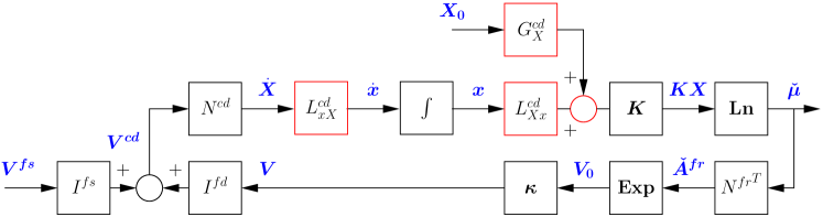
(a) Reduced-order system

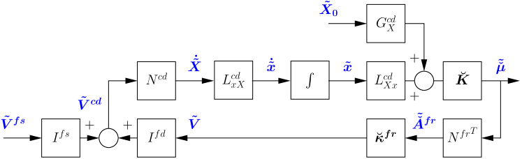
(b) Linearised Reduced-order system

Figure 4: Reduced-order system block diagrams. (a) Reduced-order system. (b) Linearised system corresponding to (a).

As discussed by number of authors [37, 38], the presence of conserved moieties leads to potential numerical difficulties with the solution of Equation (26). As chemostats introduce further conserved moieties it is important to resolve this issue. The following outline uses the notation and approach of Gawthrop and Crampin [13, §3(c)].

Defining ${G^{cd}}$ as the left null-space matrix of $N^{cd}$ it follows that:

$${G^{cd}}\dot{\boldsymbol{X}}={G^{cd}}{N^{cd}}\boldsymbol{V}=0$$ (46)

Hence each of the $n_{G}$ rows of ${G^{cd}}$ defines an algebraic relationship between the states contained in $\boldsymbol{X}$. Thus the number of independent states $n_{x}$ is given in terms of the total number of states $n_{X}$ by:

$$n_{x}=n_{X}-n_{G}$$ (47)

The derivative of the independent states $\boldsymbol{x}$ is given in terms of the derivative of state $\boldsymbol{X}$ by the $n_{x}\times n_{X}$ transformation matrix ${L^{cd}}_{xX}$

$$\dot{\boldsymbol{x}}={L^{cd}}_{xX}\dot{\boldsymbol{X}}$$ (48)

Similarly

$$\dot{\boldsymbol{X}}={L^{cd}}_{Xx}\dot{\boldsymbol{x}}$$ (49)

where ${L^{cd}}_{Xx}$ is an $n_{X}\times n_{x}$ matrix. Integrating equation (49),

$$\boldsymbol{X} ={L^{cd}}_{Xx}\boldsymbol{x}+\boldsymbol{X}_{0}-{L^{cd}}_{Xx}\boldsymbol{x}_{0}={L^{cd}}_{Xx}\boldsymbol{x}+{G^{cd}}_{X}\boldsymbol{X}_{0}$$ (50)

$$\text{where }{G^{cd}}_{X} =I_{n_{X}\times n_{X}}-{L^{cd}}_{Xx}{L^{cd}}_{xX}$$ (51)

and $\boldsymbol{x}_{0}$ and $\boldsymbol{X}_{0}$ are the values of $\boldsymbol{x}$ and $\boldsymbol{X}$ at time $t=0$.

Figure 4(a) corresponds to the open system bond graph and block diagram of Figure 3, but the reduced-order equations (48) and  (50) have been incorporated. The block ${L^{cd}}_{xX}$ contracts the state dimension from $n_{X}$ to $n_{x}$ and the block ${L^{cd}}_{Xx}$ expands it again. The initial condition term $G_{X}\boldsymbol{X}(0)$ becomes an exogenous signal analogous to the setpoint term of feedback control; note that this includes the states of all of the chemostats.

3.6 Examples

The simple reaction $A{\;\xrightleftharpoons{1}\;}B$ of Figure 1(c) has a single conserved moiety represented by

$$x_{A}+x_{B}=x_{AB}$$ (52)

where $x_{AB}$ is a constant. One possibility is

$$\boldsymbol{x} =\begin{pmatrix}x_{A}\end{pmatrix} L_{xX} =\begin{pmatrix}1&0\end{pmatrix} L_{Xx} =\begin{pmatrix}1\\ -1\end{pmatrix} G_{X} =\begin{pmatrix}0&0\\ 1&1\end{pmatrix}$$ (53)

The enzyme-catalysed reaction $A+E{\;\xrightleftharpoons{1}\;}C{\;\xrightleftharpoons{2}\;}B+E$ of Figure 2(b) has a number of possible representations depending on which C components are chemostats and which Re components are flowstats. Two of these are examined here.

Firstly, consider the case where both C:$\mathbf{A}$ and C:$\mathbf{B}$ are chemostats and Re:$\mathbf{r0}$ is a flowstat with zero flow. The relevant stoichiometric matrix is thus $N^{d}$ of Equation (45) that determines system properties and

$$N^{d} =\begin{pmatrix}0&0&0\\ 0&0&0\\ 0&1&-1\\ 0&-1&1\end{pmatrix} G^{d} =\begin{pmatrix}1&0&0&0\\ 0&1&0&0\\ 0&0&1&1\end{pmatrix}$$ (54)

$G^{d}$ has three rows corresponding to the three conserved moieties $x_{A}$, $x_{B}$ and $x_{C}+x_{E}$. The first correspond to the two chemostats, the third to the well-known conserved moiety for enzyme-catalysed reactions: the total enzyme amount is conserved. There is only one independent state which is chosen as $x_{C}$. With this choice:

$$L_{xX} =\begin{pmatrix}0&0&1&0\end{pmatrix} L_{Xx} =\begin{pmatrix}0\\ 0\\ 1\\ -1\end{pmatrix} G_{X} =\begin{pmatrix}1&0&0&0\\ 0&1&0&0\\ 0&0&0&0\\ 0&0&1&1\end{pmatrix}$$ (55)

Secondly, consider the case where both C:$\mathbf{A}$ and C:$\mathbf{B}$ are chemostats and Re:$\mathbf{r0}$ is a flowstat with non-zero flow. The relevant stoichiometric matrix is thus $N^{c}d$ of Equation (40) that determines system properties and

$$N^{cd} =\begin{pmatrix}0&0&0\\ 0&0&0\\ 0&1&-1\\ 1&-1&1\end{pmatrix} G^{cd} =\begin{pmatrix}1&0&0&0\\ 0&1&0&0\end{pmatrix}$$ (56)

The effect of the variable flowstat is to remove the third conserved moiety leaving only the chemostat states $x_{A}$ and $x_{B}$. There are now two independent states $x_{C}$ and $x_{E}$. This gives:

$$L_{xX} =\begin{pmatrix}0&0&1&0\\ 0&0&0&1\end{pmatrix} L_{Xx} =\begin{pmatrix}0&0\\ 0&0\\ 1&0\\ 0&1\end{pmatrix} G_{X} =\begin{pmatrix}1&0&0&0\\ 0&1&0&0\\ 0&0&0&0\\ 0&0&0&0\end{pmatrix}$$ (57)

4 Linearisation

As discussed in the Introduction, linearisation of non-linear systems is a standard technique in control engineering. In § 5 of this paper, linearisation is used to analyse the properties of modules.

Assuming that the system reaches a steady-state $\bar{\boldsymbol{X}}$, that is $\dot{\boldsymbol{X}}=0$ when $\boldsymbol{X}=\bar{\boldsymbol{X}}$, the system can be linearised about that steady state by introducing perturbation variables $\tilde{\boldsymbol{X}}$ so that $\boldsymbol{X}=\tilde{\boldsymbol{X}}+\bar{\boldsymbol{X}}$. These can be defined for each relevant variable; for example:

$$x =\bar{x}+\tilde{x} \mu =\bar{\mu}+\tilde{\mu} A^{f} =\bar{A^{f}}+\tilde{A^{f}} A^{r} =\bar{A^{r}}+\tilde{A^{r}} v =\bar{v}+\tilde{v}$$ (58)

If the perturbation is small, each variable can be approximated using a first-order Taylor series; thus, for example $\tilde{\mu}\approx\frac{\partial\mu}{\partial x}\tilde{x}$.

4.1 Component linearisation: C and Re

The non-linear C component is defined by the equations (11). In particular, for substance $A$:

$${\check{\mu}}_{A} =\ln K_{A}x_{A} \dot{x}_{A} =v_{A}$$ (59)

Using the perturbation approach, it follows that the linearised C component is defined by the equations:

$$\tilde{{\check{\mu}}}_{A} =\breve{K}_{A}\tilde{x}_{A} \breve{K}_{A} =\frac{\partial{\check{\mu}}_{A}}{\partial{x_{A}}}=\frac{1}{\bar{x}_{A}} \dot{\tilde{x}}_{A} =\tilde{v}_{A}$$ (60)

The non-linear Re component representing the $ith$ reaction (12) is defined by equations (16), in particular:

$$v_{i} =\kappa_{i}\left(v_{0}^{+}-v_{0}^{-}\right) v_{0}^{+} =e^{{\check{A}}^{f}_{i}} v_{0}^{-} =e^{{\check{A}}^{r}_{i}}$$ (61)

Hence the linearised Re component is defined by the equations:

$$\tilde{v}_{i} =\breve{\kappa}^{f}_{i}\tilde{{\check{A}}}^{f}_{i}-\breve{\kappa}^{r}_{i}\tilde{{\check{A}}}^{r}_{i} \breve{\kappa}^{f}_{i} =\frac{\partial v_{i}}{\partial{{\check{A}}^{f}_{i}}}=\kappa_{i}{\bar{v}_{0}^{+}} \breve{\kappa}^{r}_{i} =-\frac{\partial v_{i}}{\partial{{\check{A}}^{r}_{i}}}=\kappa_{i}\bar{v}_{0}^{-}$$ (62)

4.2 Linearised system equations

Section 4.1 shows how the bond graph components are linearised; essentially the non-linear $\exp$ and $\ln$ functions are replaced by linear gains dependent on the steady-state flows and steady-state states respectively. The $n_{X}$ constants $\breve{K}_{A},\breve{K}_{B},\dots$ of the linearised C components, and the $n_{V}$ constants $\breve{\kappa}^{f}_{1},\breve{\kappa}^{f}_{2},\dots$ and $\breve{\kappa}^{r}_{1},\breve{\kappa}^{r}_{2},\dots$ are collected into column vectors:

$$\breve{K} =\begin{pmatrix}\breve{K}_{A}\\ \breve{K}_{B}\\ \vdots\end{pmatrix} \breve{\kappa}^{f} =\begin{pmatrix}\breve{\kappa}^{f}_{1}\\ \breve{\kappa}^{f}_{2}\\ \vdots\end{pmatrix} \breve{\kappa}^{r} =\begin{pmatrix}\breve{\kappa}^{r}_{1}\\ \breve{\kappa}^{r}_{2}\\ \vdots\end{pmatrix}$$ (63)

Figure 4(b) shows the block diagram corresponding to the linearisation of the reduced-order system depicted in Figure 4(a) where:

$$\breve{\boldsymbol{K}} =\text{diag }{\breve{K}} \breve{\boldsymbol{\kappa}} =\text{diag }{\breve{\kappa}^{fr}} \text{where }\breve{\kappa}^{fr} =\begin{pmatrix}\breve{\kappa}^{f}\\ \breve{\kappa}^{r}\end{pmatrix}$$ (64)

The block diagram of the linearised version of the full system of Figure 3(d) gives the following linear state-space equations:

$$\tilde{\boldsymbol{V}} =\boldsymbol{C}\tilde{\boldsymbol{X}} \tilde{\boldsymbol{V}}^{cd} =I^{fd}\tilde{\boldsymbol{V}}+I^{fs}\tilde{\boldsymbol{V}}^{fs} \dot{\tilde{\boldsymbol{X}}} =\boldsymbol{A}\tilde{\boldsymbol{X}}+\boldsymbol{B}\tilde{\boldsymbol{V}}^{fs}$$ (65)

where

$$\boldsymbol{A} =N^{cd}I^{fd}\boldsymbol{C}=N^{d}\boldsymbol{C} \boldsymbol{B} =N^{cd}I^{fs} \boldsymbol{C} =\breve{\boldsymbol{\kappa}}^{fr}{N^{fr}}^{T}\breve{\boldsymbol{K}}$$ (66)

The block diagram of the reduced system in Figure 4(b) gives the following linear state-space equations:

$$\tilde{\boldsymbol{V}} =\boldsymbol{c}\tilde{\boldsymbol{x}}+\boldsymbol{d}\tilde{\boldsymbol{X}}_{0} \dot{\tilde{\boldsymbol{x}}} =\boldsymbol{a}\tilde{\boldsymbol{x}}+\boldsymbol{b}_{v}\tilde{\boldsymbol{V}}^{fs}+\boldsymbol{b}_{x}\tilde{\boldsymbol{X}}_{0}$$ (67)

where

$$\boldsymbol{a} =L^{cd}_{xX}\boldsymbol{A}L^{cd}_{Xx} \boldsymbol{b}_{v} =L^{cd}_{xX}\boldsymbol{B} \boldsymbol{b}_{x} =L^{cd}_{xX}\boldsymbol{A}G^{cd}_{X} \boldsymbol{c} =\boldsymbol{C}L^{cd}_{Xx} \boldsymbol{d} =\boldsymbol{C}G^{cd}_{X}$$ (68)

Equations (67) can be written more compactly as:

$$\tilde{\boldsymbol{V}} =\boldsymbol{c}\tilde{\boldsymbol{x}}+\boldsymbol{d}\tilde{\boldsymbol{U}}$$ (69)

$$\dot{\tilde{\boldsymbol{x}}} =\boldsymbol{a}\tilde{\boldsymbol{x}}+\boldsymbol{b}\tilde{\boldsymbol{U}}$$ (70)

$$\text{where }\boldsymbol{U} =\begin{pmatrix}\tilde{\boldsymbol{X}}_{0}\\ \tilde{\boldsymbol{V}}^{fs}\end{pmatrix}$$ (71)

$$\boldsymbol{b} =\begin{pmatrix}\boldsymbol{b}_{x}&\boldsymbol{b}_{v}\end{pmatrix}$$ (72)

$$\text{and }\boldsymbol{d} =\begin{pmatrix}\boldsymbol{d}_{x}&0_{n_{x}\times n_{V}}\end{pmatrix}$$ (73)

where $0_{n_{x}\times n_{V}}$ is the zero matrix with indicated dimensions.

Because the state-space systems (65) and (67) are linear, they can also be represented as transfer functions in the Laplace variable $s$. In particular, the reduced-order system (67) has the transfer function $\boldsymbol{G}(s)$ given by

$$\boldsymbol{G}(s) =\boldsymbol{c}\left(sI_{n_{x}\times n_{x}}-\boldsymbol{a}\right)^{-1}\boldsymbol{b}+\boldsymbol{d}$$ (74)

$$\text{where }\boldsymbol{V}(s) =\boldsymbol{G}(s)\boldsymbol{U}(s)$$

$I_{n_{x}\times n_{x}}$ is the unit matrix with indicated dimensions.

4.3 Examples

The simple reaction $A{\;\xrightleftharpoons{1}\;}B$ of Figure 1(c) has a flow given by (19). As both state derivatives are proportional to $v$, it follows that the steady-state is defined by: $v=\kappa\left(K_{A}x_{A}-K_{B}x_{A}\right)=0$. As noted in Equation (52), $x_{A}+x_{B}=x_{AB}$ where $x_{AB}$ is a constant. It follows that the steady-state values of $x_{A}$ and $x_{B}$ are

$$\bar{x}_{A} =\frac{K_{B}}{K_{A}+K_{B}}x_{AB} \bar{x}_{B} =\frac{K_{A}}{K_{A}+K_{B}}x_{AB}$$ (75)

From Equation (18) $v^{+}_{0}=K_{A}x_{A}$ and $v^{-}_{0}=K_{B}x_{B}$. Hence

$$\bar{v}^{+}_{0}=\bar{v}^{-}_{0}=\frac{K_{A}K_{B}}{K_{A}+K_{B}}x_{AB}$$ (76)

Using the formulae (60) and (62), it follows that the coefficients of the linearised C components are:

$$\breve{K}_{A} =\frac{1}{\bar{x}_{A}}=\frac{K_{A}+K_{B}}{K_{B}\bar{x}_{AB}} \breve{K}_{B} =\frac{1}{\bar{x}_{B}}=\frac{K_{A}+K_{B}}{K_{A}\bar{x}_{AB}}$$ (77)

and that the coefficients of the linearised Re component are:

$$\breve{\kappa}^{f}=\breve{\kappa}^{r}=\kappa\frac{K_{A}K_{B}}{K_{A}+K_{B}}x_{AB}$$ (78)

Hence the linearised equations for the flow are:

$$\tilde{v}=\breve{\kappa}^{f}\breve{K}_{A}\tilde{x}_{A}-\breve{\kappa}^{r}\breve{K}_{B}\tilde{x}_{B}=\kappa\left(K_{A}\tilde{x}_{A}-K_{B}\tilde{x}_{B}\right)$$ (79)

As expected, the linearisation of a linear equation is the same as the linear equation.

5 Modularity, Retroactivity and Feedback

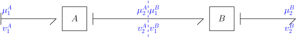
(a) Series connection: bond graph

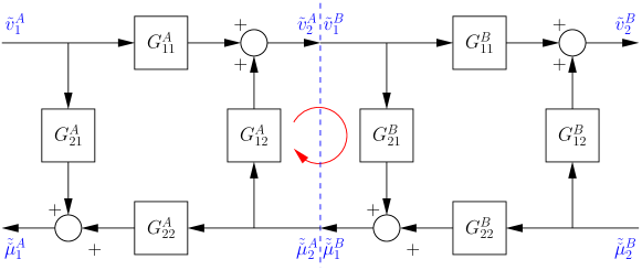
(b) Series connection: linearised block diagram

Figure 5: Modularity, Retroactivity and Feedback

Modularity provides one approach to understanding the complex systems associated with biochemical systems [39, 40, 41, 42, 43, 44]. However, as discussed by Kaltenbach and Stelling [45] there are many possible concepts of modularity. These include structure deduced from the stoichiometric matrix [46, 47]; modular construction of in silico models [48]; and modular structure designed to minimise the retroactivity between modules [45, 19, 20].

This paper focuses on two overlapping, but conceptually different concepts of modularity:

Computation modularity:

modules retain physically correct results when connected together to form a system

Behavioural modularity:

modules retain their behaviour (such as ultrasensitivity) when connected together.

Gawthrop et al. [14] have shown that bond graphs provide an effective foundation for modular construction of computer models of biochemical systems. This paper focuses on the second interpretation of modularity and shows that bond graphs provide a natural interpretation of inter-module retroactivity [15, 16, 17, 49, 50, 19, 20]. Retroactivity has been illustrated experimentally in the context of “signalling properties of a covalent modification cycle” [51], “load-induced modulation of signal transduction networks” [52] and the “temporal dynamics of gene transcription” [53]. Retroactivity can be removed using “insulation” Vecchio and Sontag [54], Sontag [49], Del Vecchio and Murray [20]; however, this may come at an energetic cost [55].

As discussed in the Introduction, feedback is another concept crucial to the understanding of complex systems. Kholodenko [22], Brightman and Fell [56], Asthagiri and Lauffenburger [57], Kolch et al. [58], Hornberg et al. [59] and Sauro and Ingalls [60] investigate the feedback in the context of MAPK cascades. As will be shown in this paper, retroactivity and feedback are closely related concepts. As will be seen, feedback arises in a number of ways including:

Intrinsic feedback

due to the interaction of reactions and species within and between modules

Conserved moieties

implicitly generate feedback loops

Feedback inhibition

explicitly uses negative feedback.

As discussed in § 4, linearisation of a non-linear system allows a wide range of control engineering techniques to be applied. In this section linearisation is used to investigate behavioural modularity using transfer functions and frequency-domain methods.

Figure 5(a) shows the series interconnection of two bond graph modules labelled $A$ and $B$. In this example, each module has two ports labelled $1$ and $2$ and the modules are interconnected to form a composite module $AB$ with two ports. To create a block diagram from a bond graph, the concept of causality is required. This concept is discussed in detail in the textbooks [3, 4, 5, 6], but here it suffices to know that causality determines which variable on a bond impinging on a system is the input, and which the output. For example, in this case the causality is such that flow $v$ is the input (and effort $\mu$ the output) on port 1 and that effort $\mu$ is the input (and flow $v$ the output) on port 2.

As discussed by Gawthrop et al. [14], the bond graph approach can be used to build arbitrarily complex systems out of such modules. However, to delve more deeply into the power of the bond graph approach and to understand how modules interact, it is instructive to look at the block diagram equivalents following linearisation as discussed in § 4. With the assumed causality, each module can be represented by four transfer functions $G_{11}$,$G_{12}$,$G_{21}$ and $G_{22}$ which can be combined into a $2\times 2$ matrix:

$$\begin{pmatrix}\tilde{v}_{2}\\ \tilde{{\check{\mu}}}_{1}\end{pmatrix}=\begin{pmatrix}G_{11}&G_{12}\\ G_{21}&G_{22}\end{pmatrix}\begin{pmatrix}\tilde{v}_{1}\\ \tilde{{\check{\mu}}}_{2}\end{pmatrix}$$ (80)

Using the superscripts $A$ and $B$ to refer to the two modules, the four transfer functions of Equation (80) can be represented for each of the interconnected modules as Figure 5(b). Connecting port 2 of $A$ to port $1$ of $B$ in Figure 5(a) is equivalent to connecting the corresponding signals in Figure 5(b):

$$\tilde{v}^{A}_{2}=\tilde{v}^{B}_{1}\text{ and }\tilde{{\check{\mu}}}^{A}_{2}=\tilde{{\check{\mu}}}^{B}_{1}$$ (81)

This connection induces a feedback loop involving $G^{A}_{12}$ and $G^{B}_{21}$ thus the properties of the composite system are dependent on the loop gain $L_{I}$ of this feedback loop.

In particular, using Equations (80) for $A$ and $B$ and substituting (81) gives the transfer function $G^{AB}$ for the composite module as

$$G^{AB}_{11} =\frac{G^{A}_{11}G^{B}_{11}}{1+L_{I}}$$ (82)

$$G^{AB}_{12} =G^{B}_{12}+\frac{G^{B}_{11}G^{A}_{12}G^{B}_{22}}{1+L_{I}}$$ (83)

$$G^{AB}_{21} =G^{A}_{21}+\frac{G^{A}_{22}G^{B}_{21}G^{A}_{11}}{1+L_{I}}$$ (84)

$$G^{AB}_{22} =\frac{G^{B}_{22}G^{A}_{22}}{1+L_{I}}$$ (85)

$$L_{I} =-G^{A}_{12}G^{B}_{21}$$ (86)

$L_{I}$ will be called the interaction loop-gain. In linear systems, feedback shifts system poles and therefore changes the behaviour of the interacting systems. In particular, each of the transfer functions $G^{AB}_{ij}$ of equations (82) – (85) is modified by the interaction loop-gain. Thus the feedback loop comprising $G^{A}_{12}$ and $G^{B}_{21}$ is the source of behaviour alteration when two modules are connected. It follows that approximate behavioural modularity is achieved by making the interaction loop-gain as small as possible. Indeed, in the special case that $G^{A}_{12}=G^{B}_{21}=0$ and so $L_{I}=0$ then:

$$G^{AB}_{11} =G^{A}_{11}G^{B}_{11}, G^{AB}_{21} =G^{A}_{21} G^{AB}_{12} =G^{B}_{12} G^{AB}_{22} =G^{B}_{22}G^{A}_{22}$$ (87)

5.1 Example module: Simple reaction

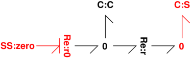
(a) With flowstat and chemostat

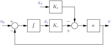
(b) Block diagram

(c) With ports

(d) Example series connection

Figure 6: Example module: simple reaction

Figure 6(a) shows a simple reaction system comprising a species represented by the C component C:$\mathbf{C}$ and the reaction component Re:$\mathbf{r}$. This closed system is converted to an open system by appending a flowstat Re:$\mathbf{r0}$ with flow $v_{0}$ and a chemostat C:$\mathbf{S}$ with state $x_{s}$. This system is linear and the reaction flow (though Re:$\mathbf{r}$) is given by:

$$v=\kappa\left(K_{c}x_{c}-K_{s}x_{s}\right)$$ (88)

and the rate of change of $x_{c}$ is

$$\dot{x}_{c}=v_{0}-v$$ (89)

Equations (88) and (89) can be visualised using the block diagram of Figure 6(b) which clearly shows the implicit feedback structure with loop gain

$$L=\frac{\kappa K_{c}}{s}$$ (90)

It follows from the block diagram of Figure 6(b) that:

$$\begin{pmatrix}v\\ x_{c}\end{pmatrix}=\frac{1}{1+L}\begin{pmatrix}L&\kappa K_{s}\\ \frac{1}{s}&\frac{\kappa K_{s}}{s}\end{pmatrix}\begin{pmatrix}v_{0}\\ x_{s}\end{pmatrix}=\frac{1}{s+\kappa K_{c}}\begin{pmatrix}\kappa K_{c}&-s\kappa K_{s}\\ 1&\kappa K_{s}\end{pmatrix}\begin{pmatrix}v_{0}\\ x_{s}\end{pmatrix}$$ (91)

In the particular case that $\kappa=K_{c}=K_{s}=1$

$$G_{11} =G_{22}=G_{21}=\frac{1}{s+1} G_{12} =\frac{-s}{s+1}$$ (92)

If two identical copies of this module are placed in series as in Figure 6(d),

$$L_{I} =\frac{s}{(s+1)^{2}} \frac{1}{1+L_{I}} =\frac{(s+1)^{2}}{s^{2}+3s+1}$$ (93)

and the resulting overall transfer function is:

$$G^{AB}_{11} =G_{22}=\frac{1}{s^{2}+3s+1} G^{AB}_{21} =\frac{-s(s+2)}{s^{2}+3s+1} G^{AB}_{12} =\frac{s+2}{s^{2}+3s+1}$$ (94)

The isolated modules each have a single pole at $s=-1$; the series modules has a pole at $s=-0.38$ and at $s=-2.62$. This shift in pole location is due to non-zero interaction loop-gain $L_{I}$ (86).

Such reaction systems are often incorrectly modelled using an irreversible reaction where the flow is independent of $\mu_{2}$. This would imply that $G_{12}=G_{22}=L=0$ and thus the overall transfer function would be

$$G^{AB}_{11} =\frac{1}{(s+1)^{2}}=\frac{1}{s^{2}+2s+1} G^{AB}_{21} =\frac{-s}{s+1} G^{AB}_{12} =G^{AB}_{22}=0$$ (95)

This thermodynamically incorrect system has zero retroactivity. As will be shown in the sequel, approximate irreversibility, and thus approximate zero retroactivity, can be achieved but at the metabolic cost of using a power supply such as that provided by the $ATP{\;\xrightleftharpoons{}\;}ADP+Pi$ reaction.

5.2 Example module: Enzyme-catalysed reaction

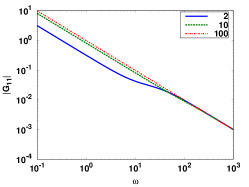
(a) $|G_{11}(j\omega)|$

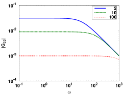
(b) $|G_{22}(j\omega)|$

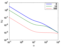
(c) $|L_{I}(j\omega)|=|G_{12}(j\omega)G_{21}(j\omega)|$

Figure 7: Example module: Enzyme-catalysed reaction. The three frequency responses are plotted for $K_{A}=2,10,100$ against frequency $\omega~{}($~{}\mathrm{r}\mathrm{a}\mathrm{d}\,\mathrm{s}\mathrm{e}\mathrm{c}^{-1}$)$.

As an example, the enzyme-catalysed reaction of Figure 2(b) is considered as a two-port module (as illustrated in Figure 5). In particular, the flowstat corresponding to Re:$\mathbf{r0}$ is replaced by port 1 and the chemostat corresponding to C:$\mathbf{B}$ is replaced by port 2. Thus Equation (80) becomes:

$$\begin{pmatrix}\tilde{v}_{2}\\ \tilde{{\check{\mu}}}_{E}\end{pmatrix}=\begin{pmatrix}G_{11}&G_{12}\\ G_{21}&G_{22}\end{pmatrix}\begin{pmatrix}\tilde{v}_{0}\\ \tilde{{\check{\mu}}}_{B}\end{pmatrix}$$ (96)

The system parameters were $K_{B}=K_{C}=K_{E}=1$, $\kappa_{1}=10$ and $\kappa_{2}=1$. Three alternative values were used for $K_{A}$: $2$, $10$ and $100$. Using an initial state $\boldsymbol{X}_{0}=\left(100\;1\;0\;1\right)^{T}$, the steady states were found for each value of $K_{A}$ and the system was linearised using the method of § 4. The transfer functions for the three cases were found to be:

$$G_{2} =\begin{pmatrix}\frac{-s+10}{s^{2}+32s}&\frac{-0.34s-10.31}{s+32}\\ \frac{2.91s+32}{s^{2}+32s}&\frac{-1}{s+32}\\ \end{pmatrix}$$ (97)

$$G_{10} =\begin{pmatrix}\frac{-s+90}{s^{2}+112s}&\frac{-0.10s-10.80}{s+112}\\ \frac{10.18s+112}{s^{2}+112s}&\frac{-1}{s+112}\\ \end{pmatrix}$$ (98)

$$G_{100} =\begin{pmatrix}\frac{-s+990}{s^{2}+1012s}&\frac{-0.01s-10.98}{s+1012}\\ \frac{92s+1012}{s^{2}+1012s}&\frac{-1}{s+1012}\\ \end{pmatrix}$$ (99)

Although these transfer functions are simple enough to analyse directly, in more complex cases it is useful to look at the transfer function frequency responses obtained by replacing the Laplace variable $s$ by $j\omega$ where $j=\sqrt{-1}$ and $\omega$ is a frequency in $\mathrm{r}\mathrm{a}\mathrm{d}\,\mathrm{s}\mathrm{e}\mathrm{c}^{-1}$. Figure 7 gives the frequency response magnitude of the three transfer functions: $G_{11}$ relating $\tilde{v}_{0}$ to $\tilde{v}_{2}$, $G_{22}$ relating $\tilde{{\check{\mu}}}_{B}$ to $\tilde{{\check{\mu}}}_{E}$ and the loop-interaction $L_{I}=-G_{12}G_{21}$. for each of the three cases.

The forward transfer function $G_{11}$ approaches $\frac{1}{s}$ as $K_{A}$ increases, the transfer functions $G_{22}$ and $L_{I}$ decrease as $K_{A}$ increases. Thus larger values of $K_{A}$ give approximate behavioural modularity. However, this comes at an energetic cost measured by the external flow associated with the chemostat C:$\mathbf{A}$.

5.3 Example module: Phosphorylation/dephosphorylation

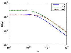
(a) $|G_{11}(j\omega)|$

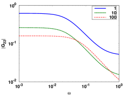
(b) $|G_{22}(j\omega)|$

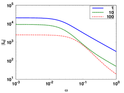
(c) $|L_{I}(j\omega)|=|G_{12}(j\omega)G_{21}(j\omega)|$

Figure 8: Example module: Phosphorylation/dephosphorylation

A bond graph model of the thermodynamically correct formulation of the phosphorylation/dephosphorylation cycle of Beard and Qian [61] was presented by Gawthrop and Crampin [13]. Figure 9(a) shows a modular version where the two ports are given by flowstat Re:$\mathbf{r0}$ and the chemostat C:$\mathbf{MP}$. The three components representing $ATP$, $ADP$ and $Pi$ (C:$\mathbf{ATP}$,C:$\mathbf{ADP}$ and C:$\mathbf{P}$) are also chemostats and provide the power source for the module.

As in § 5.2, this module can be analysed by plotting the frequency response of the three transfer functions. The parameters (which are illustrative and do not correspond to a specific biological instance) are:

$$\boldsymbol{X} =\begin{pmatrix}x_{E1}\\ x_{C1}\\ x_{E2}\\ x_{C2}\\ x_{ATP}\\ x_{ADP}\\ x_{P}\\ x_{M}\\ x_{MP}\\ \end{pmatrix} \boldsymbol{X}_{0} =\begin{pmatrix}0\\ 0\\ 0.001\\ 0\\ 1,10,100\\ 1\\ 0.01\\ 10\\ 0\\ \end{pmatrix} K =\begin{pmatrix}100\\ 1\\ 100\\ 1\\ 0.1\\ 0.001\\ 0.001\\ 1\\ 1\\ \end{pmatrix} \kappa =\begin{pmatrix}10\\ 1000\\ 10\\ 1000\\ \end{pmatrix}$$ (100)

The (fixed) amount of $ATP$ was set at three alternative values: $x_{ATP}=1,10,100$. As in § 5.2, larger values give reduced loop interaction at the expense of more power needed to drive the module.

5.4 Example module: Feedback inhibition

The idea that a product can inhibit an enzyme and thus give negative feedback is a well-established concept in biology [62, 63, 64, 65]. This section focuses on one possible mechanism, competitive inhibition [66, § 1.4.3]. The basic idea is that the product $P$ binds to the enzyme $E$ to form a complex $C$ (thus partially sequestering $E$) via the reaction:

$$P+E{\;\xrightleftharpoons{}\;}C$$ (101)

Together with an additional flow of enzyme modelled by Re:$\mathbf{r0}$, this reaction is modelled by the bond graph of Figure 10(a). This can be represented as a two-port module if C:$\mathbf{P}$, Re:$\mathbf{r0}$ and associated junctions are replaced by ports. This module will be used in the sequel to apply feedback inhibition to the MAPK cascade.

6 MAPK cascades.

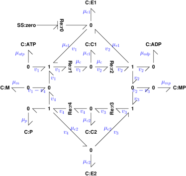
(a) Phosphorylation/dephosphorylation

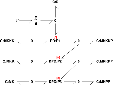
(b) MAPK cascade

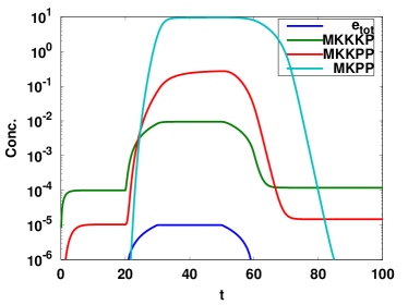
(c) Time courses

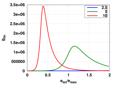
(d) Effect of $ATP$

Figure 9: MAPK cascade: modular model

The mitogen-activated protein kinase (MAPK) cascade is a well-studied signalling pathway with ultrasensitive components [21, 22, 58]. However, the use of the Michaelis-Menten approximation to enzyme-catalysed reactions can be misleading in this context. In particular, as discussed by Voit [67, §9.5], “It is tempting to set up the two phosphorylation steps with Michaelis-Menten rate functions, but such a strategy is not the best option, because (1) the enzyme concentration is not constant, (2) the enzyme concentration is not necessarily smaller than the substrate concentration, and (3) the two reaction steps are competing for the same enzyme.”.

This section shows that the bond graph property of computational modularity can be used to build a computational model of the MAPK cascade which is thermodynamically correct and thus avoids the pitfalls associated with inappropriate use of the Michaelis-Menten approximation. Moreover, having seen in § 5.3 that that the bond graph module corresponding to phosphorylation/dephosphorylation can be designed to give approximate behavioural modularity, the MAPK cascade can be built with approximate behavioural modularity.

Figure 9(b) shows the bond graph of the MAPK cascade based on the phosphorylation/dephosphorylation module PD of Figure 8 and the double phosphorylation/dephosphorylation module DPD the Re:$\mathbf{r0}$ component is used as a flowstat generating a flow $v_{0}$ as discussed in Section 5.2. The nonlinear system of ODEs corresponding to Figure 9(b) was simulated for 100 time units with an input $v_{0}$ given by

$$v_{0}=\begin{cases}10^{-6}&20\geq t\geq 30\\ -10^{-6}&50\geq t\geq 60\\ 0&\text{otherwise}\end{cases}$$ (102)

This gives a maximum value of the total enzyme of $e_{max}=10^{-5}$. The system parameters are those used in § 5.3.

Figure 9(c) shows the corresponding time courses for the total amount of enzyme $e_{tot}$, and the amounts of $MKKKP$, $MKKPP$ and $MKPP$. A logarithmic scale is used to account for the large range of values. Note that the gain between $e_{tot}$ and the concentration $x_{MKPP}$ is of the order of $10^{6}$.

The steady-state value of $x_{MKPP}$ was computed for a range of values of $e_{tot}$ and the incremental values $\frac{dx_{MKPP}}{de_{tot}}$ were computed numerically for three values of $ATP$: $x_{ATP}=2.5,5,10$. Figure 9(d) shows the incremental gain plotted against $e_{tot}$. The high gain due to the ultrasensitivity of the phosphorylation/dephosphorylation modules vanishes between $ATP$ amounts of $2$ and $5$.

(a) Feedback inhibition

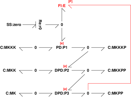
(b) MAPK cascade with feedback inhibition

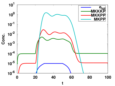
(c) Time courses

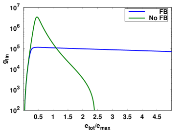
(d) Incremental gains.

Figure 10: MAPK cascade with feedback inhibition

In his seminal paper Black [68] points out that “by building an amplifier whose gain is deliberately made, say 40 decibels higher than necessary …, and then feeding the output back on the input in such a way as to throw away the excess gain, it has been found possible to effect extraordinary improvement in constancy of amplification and freedom from non-linearity.” In this context, Figure 10(b) is the same as Figure 9(b) except that the feedback inhibition module of § 5.4 is incorporated in to the bond graph and the system is re-simulated with $K_{fi}=4$ and $\kappa_{fi}=1$.

The steady-state value of $x_{MKPP}$ was computed for a range of values of $e_{tot}$ and the incremental values $\frac{dx_{MKPP}}{de_{tot}}$ were computed numerically both with and without feedback and plotted in Figure 10(d). The gain of the system is reduced by a factor of about $20$ but the system is now more linear: the gain is approximately constant over a wider range of $e_{tot}$ than was the case without feedback.

7 Conclusion

Building on its inherent computational modularity; it has been shown that the bond graph approach can be used to explain and adjust behavioural modularity. The MAPK cascade was used as an example to illustrate this point. It would be interesting to repeat the MAPK examples with parameter values taken from the literature [69, 70]. This may provide insight into the evolutionary trade-off between energy consumption and signalling performance [71, 72, 73].

Control-theoretic concepts based on linearisation were shown to provide a quantitative analysis of behavioural modularity. However, nonlinear systems can be approximated in other ways apart from linearisation. In the context of metabolic network modelling, Heijnen [74] discusses and compares a number of approximations including: logarithmic-linear, power law generalised mass action, S-systems [63, 67] and linear logarithmic [75, 76]. It would be interesting to see whether such approximations provide an alternative to linearisation in analysing behavioural modularity.

It has been suggested that metabolism and its dysfunctions may related to certain diseases including Parkinson’s disease [77, 78], heart disease [79], cancer [80, 81] and chronic fatigue [82]. It is envisaged the the energy-based approach used in this paper will help to understand such energy-related diseases.

The example in this paper examines a signalling network as an analogy to an electronic amplifier. Gene regulatory networks have been analysed and synthesised as amplifiers [83, 84, 85]. Future work will examine the bond graph based analysis and synthesis of gene regulatory networks.

Acknowledgements

Peter Gawthrop would like to thank the Melbourne School of Engineering for its support via a Professorial Fellowship. This research was in part conducted and funded by the Australian Research Council Centre of Excellence in Convergent Bio-Nano Science and Technology (project number CE140100036).

References

- Wellstead et al. [2008] Peter Wellstead, Eric Bullinger, Dimitrios Kalamatianos, Oliver Mason, and Mark Verwoerd. The role of control and system theory in systems biology. Annual Reviews in Control, 32(1):33 – 47, 2008. ISSN 1367-5788. doi:DOI: 10.1016/j.arcontrol.2008.02.001.
- Paynter [1961] H. M. Paynter. Analysis and design of engineering systems. MIT Press, Cambridge, Mass., 1961.
- Wellstead [1979] P. E. Wellstead. Introduction to Physical System Modelling. Academic Press, 1979.
- Gawthrop and Smith [1996] P. J. Gawthrop and L. P. S. Smith. Metamodelling: Bond Graphs and Dynamic Systems. Prentice Hall, Hemel Hempstead, Herts, England., 1996. ISBN 0-13-489824-9.
- Mukherjee et al. [2006] Amalendu Mukherjee, Ranjit Karmaker, and Arun Kumar Samantaray. Bond Graph in Modeling, Simulation and Fault Indentification. I.K. International, New Delhi,, 2006.
- Karnopp et al. [2012] Dean C Karnopp, Donald L Margolis, and Ronald C Rosenberg. System Dynamics: Modeling, Simulation, and Control of Mechatronic Systems. John Wiley & Sons, 5th edition, 2012. ISBN 978-0470889084.
- Gawthrop and Bevan [2007] Peter J Gawthrop and Geraint P Bevan. Bond-graph modeling: A tutorial introduction for control engineers. IEEE Control Systems Magazine, 27(2):24–45, April 2007. doi:10.1109/MCS.2007.338279.
- Oster et al. [1971] George Oster, Alan Perelson, and Aharon Katchalsky. Network thermodynamics. Nature, 234:393–399, December 1971. doi:10.1038/234393a0.
- Oster et al. [1973] George F. Oster, Alan S. Perelson, and Aharon Katchalsky. Network thermodynamics: dynamic modelling of biophysical systems. Quarterly Reviews of Biophysics, 6(01):1–134, 1973. doi:10.1017/S0033583500000081.
- Cellier [1991] F. E. Cellier. Continuous system modelling. Springer-Verlag, 1991.
- Thoma and Mocellin [2006] Jean U. Thoma and Gianni Mocellin. Simulation with Entropy Thermodynamics: Understanding Matter and Systems with Bondgraphs. Springer, 2006. ISBN 978-3-540-32798-1.
- Greifeneder and Cellier [2012] J. Greifeneder and F.E. Cellier. Modeling chemical reactions using bond graphs. In Proceedings ICBGM12, 10th SCS Intl. Conf. on Bond Graph Modeling and Simulation, pages 110–121, Genoa, Italy, 2012.
- Gawthrop and Crampin [2014] Peter J. Gawthrop and Edmund J. Crampin. Energy-based analysis of biochemical cycles using bond graphs. Proceedings of the Royal Society A: Mathematical, Physical and Engineering Science, 470(2171):1–25, 2014. doi:10.1098/rspa.2014.0459. Available at arXiv:1406.2447.
- Gawthrop et al. [2015] Peter J. Gawthrop, Joseph Cursons, and Edmund J. Crampin. Hierarchical bond graph modelling of biochemical networks. Proceedings of the Royal Society A: Mathematical, Physical and Engineering Sciences, 471(2184):1–23, 2015. ISSN 1364-5021. doi:10.1098/rspa.2015.0642. Available at arXiv:1503.01814.
- Saez-Rodriguez et al. [2004] J. Saez-Rodriguez, Andreas Kremling, H. Conzelmann, K. Bettenbrock, and E.D. Gilles. Modular analysis of signal transduction networks. Control Systems, IEEE, 24(4):35–52, Aug 2004. ISSN 1066-033X. doi:10.1109/MCS.2004.1316652.
- Saez-Rodriguez et al. [2005] J. Saez-Rodriguez, A. Kremling, and E.D. Gilles. Dissecting the puzzle of life: modularization of signal transduction networks. Computers and Chemical Engineering, 29(3):619 – 629, 2005. ISSN 0098-1354. doi:10.1016/j.compchemeng.2004.08.035. Computational Challenges in Biology.
- Del Vecchio et al. [2008] Domitilla Del Vecchio, Alexander J. Ninfa, and Eduardo D. Sontag. Modular cell biology: retroactivity and insulation. Molecular Systems Biology, 4:1–16, 2008. doi:10.1038/msb4100204.
- Ossareh et al. [2011] Hamid R. Ossareh, Alejandra C. Ventura, Sofia D. Merajver, and Domitilla Del Vecchio. Long signaling cascades tend to attenuate retroactivity. Biophysical Journal, 100(7):1617 – 1626, 2011. ISSN 0006-3495. doi:10.1016/j.bpj.2011.02.014.
- Del Vecchio [2013] Domitilla Del Vecchio. A control theoretic framework for modular analysis and design of biomolecular networks. Annual Reviews in Control, 37(2):333 – 345, 2013. ISSN 1367-5788. doi:10.1016/j.arcontrol.2013.09.011.
- Del Vecchio and Murray [2014] Domitilla Del Vecchio and Richard M Murray. Biomolecular Feedback Systems. Princeton University Press, 2014. ISBN 0691161534.
- Huang and Ferrell [1996] C Y Huang and J E Ferrell. Ultrasensitivity in the mitogen-activated protein kinase cascade. Proceedings of the National Academy of Sciences, 93(19):10078–10083, 1996.
- Kholodenko [2000] Boris N. Kholodenko. Negative feedback and ultrasensitivity can bring about oscillations in the mitogen-activated protein kinase cascades. European Journal of Biochemistry, 267(6):1583–1588, 2000. ISSN 1432-1033. doi:10.1046/j.1432-1327.2000.01197.x.
- Ortega et al. [2002] Fernando Ortega, Luis Acerenza, Hans V. Westerhoff, Francesca Mas, and Marta Cascante. Product dependence and bifunctionality compromise the ultrasensitivity of signal transduction cascades. Proceedings of the National Academy of Sciences, 99(3):1170–1175, 2002. doi:10.1073/pnas.022267399.
- Bluthgen et al. [2006] Nils Bluthgen, Frank J. Bruggeman, Stefan Legewie, Hanspeter Herzel, Hans V. Westerhoff, and Boris N. Kholodenko. Effects of sequestration on signal transduction cascades. FEBS Journal, 273(5):895–906, 2006. ISSN 1742-4658. doi:10.1111/j.1742-4658.2006.05105.x.
- Goodwin et al. [2001] G.C. Goodwin, S.F. Graebe, and M.E. Salgado. Control System Design. Prentice Hall, Englewood Cliffs, New Jersey, 2001.
- Karnopp [1977] Dean Karnopp. Power and energy in linearized physical systems. Journal of the Franklin Institute, 303(1):85 – 98, 1977. ISSN 0016-0032. doi:10.1016/0016-0032(77)90078-3.
- Gawthrop [2000] Peter J Gawthrop. Sensitivity bond graphs. Journal of the Franklin Institute, 337(7):907–922, November 2000. doi:10.1016/S0016-0032(00)00052-1.
- Borutzky [2011] Wolfgang Borutzky. Incremental bond graphs. In Wolfgang Borutzky, editor, Bond Graph Modelling of Engineering Systems, pages 135–176. Springer New York, 2011. ISBN 978-1-4419-9367-0. doi:10.1007/978-1-4419-9368-7_4.
- Maxwell [1871] J.C. Maxwell. Remarks on the mathematical classification of physical quantities. Proceedings London Mathematical Society, pages 224–233, 1871.
- Atkins and de Paula [2011] Peter Atkins and Julio de Paula. Physical Chemistry for the Life Sciences. Oxford University Press, 2nd edition, 2011.
- Job and Herrmann [2006] G Job and F Herrmann. Chemical potential – a quantity in search of recognition. European Journal of Physics, 27(2):353–371, 2006. doi:10.1088/0143-0807/27/2/018.
- Van Rysselberghe [1958] Pierre Van Rysselberghe. Reaction rates and affinities. The Journal of Chemical Physics, 29(3):640–642, 1958. doi:10.1063/1.1744552.
- Palsson [2006] Bernhard Palsson. Systems biology: properties of reconstructed networks. Cambridge University Press, 2006. ISBN 0521859034.
- van der Schaft et al. [2013] A. van der Schaft, S. Rao, and B. Jayawardhana. On the mathematical structure of balanced chemical reaction networks governed by mass action kinetics. SIAM Journal on Applied Mathematics, 73(2):953–973, 2013. doi:10.1137/11085431X.
- Polettini and Esposito [2014] Matteo Polettini and Massimiliano Esposito. Irreversible thermodynamics of open chemical networks. I. Emergent cycles and broken conservation laws. The Journal of Chemical Physics, 141(2):024117, 2014. doi:10.1063/1.4886396.
- Qian and Beard [2005] Hong Qian and Daniel A. Beard. Thermodynamics of stoichiometric biochemical networks in living systems far from equilibrium. Biophysical Chemistry, 114(2-3):213 – 220, 2005. ISSN 0301-4622. doi:10.1016/j.bpc.2004.12.001.
- Sauro [2009] H.M. Sauro. Network dynamics. In Rene Ireton, Kristina Montgomery, Roger Bumgarner, Ram Samudrala, and Jason McDermott, editors, Computational Systems Biology, volume 541 of Methods in Molecular Biology, pages 269–309. Humana Press, New York, 2009. ISBN 978-1-58829-905-5. doi:10.1007/978-1-59745-243-4-13.
- Ingalls [2013] Brian P. Ingalls. Mathematical Modelling in Systems Biology. MIT Press, 2013.
- Hartwell et al. [1999] Leland H Hartwell, John J Hopfield, Stanislas Leibler, and Andrew W Murray. From molecular to modular cell biology. Nature, 402:C47–C52, 1999.
- Lauffenburger [2000] Douglas A. Lauffenburger. Cell signaling pathways as control modules: Complexity for simplicity? Proceedings of the National Academy of Sciences, 97(10):5031–5033, 2000. doi:10.1073/pnas.97.10.5031.
- Csete and Doyle [2002] Marie E. Csete and John C. Doyle. Reverse engineering of biological complexity. Science, 295(5560):1664–1669, 2002. doi:10.1126/science.1069981.
- Bruggeman et al. [2002] Frank J. Bruggeman, Hans V. Westerhoff, Jan B. Hoek, and Boris N. Kholodenko. Modular response analysis of cellular regulatory networks. Journal of Theoretical Biology, 218(4):507 – 520, 2002. ISSN 0022-5193. doi:10.1006/jtbi.2002.3096.
- Bruggeman et al. [2008] F.J. Bruggeman, J.L. Snoep, and H.V. Westerhoff. Control, responses and modularity of cellular regulatory networks: a control analysis perspective. Systems Biology, IET, 2(6):397–410, November 2008. ISSN 1751-8849. doi:10.1049/iet-syb:20070065.
- Szallasi et al. [2010] Z. Szallasi, V. Periwal, and Jorg Stelling. On modules and modularity. In Z. Szallasi, J. Stelling, and V. Periwal, editors, System Modeling in Cellular Biology: From Concepts to Nuts and Bolts, pages 19–40. MIT press, 2010.
- Kaltenbach and Stelling [2012] Hans-Michael Kaltenbach and Jorg Stelling. Modular analysis of biological networks. In Igor I. Goryanin and Andrew B. Goryachev, editors, Advances in Systems Biology, volume 736 of Advances in Experimental Medicine and Biology, pages 3–17. Springer New York, 2012. ISBN 978-1-4419-7209-5. doi:10.1007/978-1-4419-7210-1_1.
- Schuster et al. [2000] Stefan Schuster, Boris N. Kholodenko, and Hans V. Westerhoff. Cellular information transfer regarded from a stoichiometry and control analysis perspective. Biosystems, 55(1–3):73 – 81, 2000. ISSN 0303-2647. doi:10.1016/S0303-2647(99)00085-4.
- Poolman et al. [2007] Mark G. Poolman, Cristiana Sebu, Michael K. Pidcock, and David A. Fell. Modular decomposition of metabolic systems via null-space analysis. Journal of Theoretical Biology, 249(4):691 – 705, 2007. ISSN 0022-5193. doi:10.1016/j.jtbi.2007.08.005.
- Neal et al. [2014] Maxwell L. Neal, Michael T. Cooling, Lucian P. Smith, Christopher T. Thompson, Herbert M. Sauro, Brian E. Carlson, Daniel L. Cook, and John H. Gennari. A reappraisal of how to build modular, reusable models of biological systems. PLoS Comput Biol, 10(10):e1003849, 10 2014. doi:10.1371/journal.pcbi.1003849.
- Sontag [2011] Eduardo D. Sontag. Modularity, retroactivity, and structural identification. In Heinz Koeppl, Gianluca Setti, Mario di Bernardo, and Douglas Densmore, editors, Design and Analysis of Biomolecular Circuits, pages 183–200. Springer New York, 2011. ISBN 978-1-4419-6765-7. doi:10.1007/978-1-4419-6766-4_9.
- Jayanthi and Del Vecchio [2011] S. Jayanthi and Domitilla Del Vecchio. Retroactivity attenuation in bio-molecular systems based on timescale separation. Automatic Control, IEEE Transactions on, 56(4):748–761, April 2011. ISSN 0018-9286. doi:10.1109/TAC.2010.2069631.
- Ventura et al. [2010] Alejandra C. Ventura, Peng Jiang, Lauren Van Wassenhove, Domitilla Del Vecchio, Sofia D. Merajver, and Alexander J. Ninfa. Signaling properties of a covalent modification cycle are altered by a downstream target. Proceedings of the National Academy of Sciences, 107(22):10032–10037, 2010. doi:10.1073/pnas.0913815107.
- Jiang et al. [2011] Peng Jiang, Alejandra C. Ventura, Eduardo D. Sontag, Sofia D. Merajver, Alexander J. Ninfa, and Domitilla Del Vecchio. Load-induced modulation of signal transduction networks. Science Signaling, 4(194):ra67–ra67, 2011. ISSN 1945-0877. doi:10.1126/scisignal.2002152.
- Jayanthi et al. [2013] Shridhar Jayanthi, Kayzad Soli Nilgiriwala, and Domitilla Del Vecchio. Retroactivity controls the temporal dynamics of gene transcription. ACS Synthetic Biology, 2(8):431–441, 2013. doi:10.1021/sb300098w.
- Vecchio and Sontag [2009] Domitilla Del Vecchio and Eduardo D. Sontag. Engineering principles in bio-molecular systems: From retroactivity to modularity. European Journal of Control, 15(3–4):389 – 397, 2009. ISSN 0947-3580. doi:10.3166/ejc.15.389-397.
- Barton and Sontag [2012] John Barton and Eduardo D Sontag. The energy costs of biological insulators. arXiv preprint arXiv:1210.3809, 2012.
- Brightman and Fell [2000] Frances A Brightman and David A Fell. Differential feedback regulation of the MAPK cascade underlies the quantitative differences in EGF and NGF signalling in PC12 cells. FEBS Letters, 482(3):169 – 174, 2000. ISSN 0014-5793. doi:10.1016/S0014-5793(00)02037-8.
- Asthagiri and Lauffenburger [2001] Anand R. Asthagiri and Douglas A. Lauffenburger. A computational study of feedback effects on signal dynamics in a mitogen-activated protein kinase (MAPK) pathway model. Biotechnology Progress, 17(2):227–239, 2001. ISSN 1520-6033. doi:10.1021/bp010009k.
- Kolch et al. [2005] Walter Kolch, Muffy Calder, and David Gilbert. When kinases meet mathematics: the systems biology of MAPK signalling. FEBS Letters, 579(8):1891 – 1895, 2005. ISSN 0014-5793. doi:DOI: 10.1016/j.febslet.2005.02.002. Systems Biology.
- Hornberg et al. [2005] Jorrit J. Hornberg, Bernd Binder, Frank J. Bruggeman, Birgit Schoeberl, Reinhart Heinrich, and Hans V. Westerhoff. Control of MAPK signalling: from complexity to what really matters. Oncogene, 24:5533–5542, June 2005. ISSN 0950-9232. doi:10.1038/sj.onc.1208817.
- Sauro and Ingalls [2007] Herbert M Sauro and Brian Ingalls. MAPK cascades as feedback amplifiers. arXiv preprint arXiv:0710.5195, 2007.
- Beard and Qian [2010] Daniel A Beard and Hong Qian. Chemical biophysics: quantitative analysis of cellular systems. Cambridge University Press, 2010.
- Monod et al. [1963] Jacques Monod, Jean-Pierre Changeux, and Francois Jacob. Allosteric proteins and cellular control systems. Journal of Molecular Biology, 6(4):306 – 329, 1963. ISSN 0022-2836. doi:10.1016/S0022-2836(63)80091-1.
- Savageau [2009] Michael A. Savageau. Biochemical Systems Analysis. A Study of Function and Design in Molecular Biology. Addison-Wesley, Reading, Mass., 40th anniversary issue edition, 2009.
- Fell [1997] David Fell. Understanding the control of metabolism, volume 2 of Frontiers in Metabolism. Portland press, London, 1997. ISBN 1 85578 047 X.
- Cornish-Bowden [2013] Athel Cornish-Bowden. Fundamentals of enzyme kinetics. Wiley-Blackwell, London, 4th edition, 2013. ISBN 978-3-527-33074-4.
- Keener and Sneyd [2009] James P Keener and James Sneyd. Mathematical Physiology: I: Cellular Physiology, volume 1. Springer, 2nd edition, 2009.
- Voit [2013] Eberhard O. Voit. A First Course in Systems Biology. Garland Science, New York and London, 2013.
- Black [1934] H.S. Black. Stabilized feedback amplifiers. The Bell System Technical Journal, 13(1):1–18, Jan 1934. ISSN 0005-8580. doi:10.1002/j.1538-7305.1934.tb00652.x.
- Nguyen et al. [2013] Lan K. Nguyen, David Matallanas, David R. Croucher, Alexander von Kriegsheim, and Boris N. Kholodenko. Signalling by protein phosphatases and drug development: a systems-centred view. FEBS Journal, 280(2):751–765, 2013. ISSN 1742-4658. doi:10.1111/j.1742-4658.2012.08522.x.
- Ahmed et al. [2014] Shoeb Ahmed, Kyle G Grant, Laura E Edwards, Anisur Rahman, Murat Cirit, Michael B Goshe, and Jason M Haugh. Data-driven modeling reconciles kinetics of ERK phosphorylation, localization, and activity states. Molecular systems biology, 10(1):718, 2014.
- Hasenstaub et al. [2010] Andrea Hasenstaub, Stephani Otte, Edward Callaway, and Terrence J. Sejnowski. Metabolic cost as a unifying principle governing neuronal biophysics. Proceedings of the National Academy of Sciences, 107(27):12329–12334, 2010. doi:10.1073/pnas.0914886107.
- de Atauri et al. [2004] P. de Atauri, D. Orrell, S. Ramsey, and H. Bolouri. Evolution of design principles in biochemical networks. Systems Biology, IEE Proceedings, 1(1):28–40, June 2004. ISSN 1741-2471. doi:10.1049/sb:20045013.
- Albergante et al. [2014] Luca Albergante, J Julian Blow, and Timothy J Newman. Buffered qualitative stability explains the robustness and evolvability of transcriptional networks. eLife, 3:1–28, 2014. doi:10.7554/eLife.02863.
- Heijnen [2005] Joseph J. Heijnen. Approximative kinetic formats used in metabolic network modeling. Biotechnology and Bioengineering, 91(5):534–545, 2005. ISSN 1097-0290. doi:10.1002/bit.20558.
- Wang et al. [2007] Feng-Sheng Wang, Chih-Lung Ko, and Eberhard O. Voit. Kinetic modeling using S-systems and lin-log approaches. Biochemical Engineering Journal, 33(3):238 – 247, 2007. ISSN 1369-703X. doi:10.1016/j.bej.2006.11.002.
- Berthoumieux et al. [2011] Sara Berthoumieux, Matteo Brilli, Hidde de Jong, Daniel Kahn, and Eugenio Cinquemani. Identification of metabolic network models from incomplete high-throughput datasets. Bioinformatics, 27(13):i186–i195, 2011. doi:10.1093/bioinformatics/btr225.
- Cloutier et al. [2012] M. Cloutier, R. Middleton, and P. Wellstead. Feedback motif for the pathogenesis of Parkinson’s disease. Systems Biology, IET, 6(3):86–93, June 2012. ISSN 1751-8849. doi:10.1049/iet-syb.2011.0076.
- Wellstead [2012] Peter Wellstead. A New Look at Disease: Parkinson’s through the eyes of an engineer. Control Systems Principles, Stockport, UK, 2012. ISBN 978-0-9573864-0-2.
- Neubauer [2007] Stefan Neubauer. The failing heart – an engine out of fuel. New England Journal of Medicine, 356(11):1140–1151, 2007. doi:10.1056/NEJMra063052.
- Masoudi-Nejad and Asgari [2014] Ali Masoudi-Nejad and Yazdan Asgari. Metabolic cancer biology: structural-based analysis of cancer as a metabolic disease, new sights and opportunities for disease treatment. Seminars in cancer biology, 30:21–29, 2014.
- Yizhak et al. [2014] Keren Yizhak, Sylvia E Le Dévédec, Vasiliki Maria Rogkoti, Franziska Baenke, Vincent C de Boer, Christian Frezza, Almut Schulze, Bob van de Water, and Eytan Ruppin. A computational study of the Warburg effect identifies metabolic targets inhibiting cancer migration. Molecular Systems Biology, 10(8), 2014. ISSN 1744-4292. doi:10.15252/msb.20134993.
- Morris and Maes [2013] Gerwyn Morris and Michael Maes. A neuro-immune model of myalgic encephalomyelitis/chronic fatigue syndrome. Metabolic Brain Disease, 28(4):523–540, 2013. ISSN 0885-7490. doi:10.1007/s11011-012-9324-8.
- Zhang et al. [2007] David Yu Zhang, Andrew J. Turberfield, Bernard Yurke, and Erik Winfree. Engineering entropy-driven reactions and networks catalyzed by dna. Science, 318(5853):1121–1125, 2007. doi:10.1126/science.1148532.
- Bath and Turberfield [2007] Jonathan Bath and Andrew J. Turberfield. DNA nanomachines. Nat Nano, 2:275–284, May 2007. ISSN 1748-3387. doi:10.1038/nnano.2007.104.
- Nakakuki [2015] Takashi Nakakuki. A multifunctional controller realized by biochemical reactions. SICE Journal of Control, Measurement, and System Integration, 8(2):99–107, 2015. doi:10.9746/jcmsi.8.99.