Estimating the number of unseen species:
A bird in the hand is worth $\log n$ in the bush

Abstract

Estimating the number of unseen species is an important problem in many scientific endeavors. Its most popular formulation, introduced by Fisher, uses $n$ samples to predict the number $U$ of hitherto unseen species that would be observed if $t\cdot n$ new samples were collected. Of considerable interest is the largest ratio $t$ between the number of new and existing samples for which $U$ can be accurately predicted.

In seminal works, Good and Toulmin constructed an intriguing estimator that predicts $U$ for all $t\leq 1$, thereby showing that the number of species can be estimated for a population twice as large as that observed. Subsequently Efron and Thisted obtained a modified estimator that empirically predicts $U$ even for some $t>1$, but without provable guarantees.

We derive a class of estimators that provably predict $U$ not just for constant $t>1$, but all the way up to $t$ proportional to $\log n$. This shows that the number of species can be estimated for a population $\log n$ times larger than that observed, a factor that grows arbitrarily large as $n$ increases. We also show that this range is the best possible and that the estimators’ mean-square error is optimal up to constants for any $t$. Our approach yields the first provable guarantee for the Efron-Thisted estimator and, in addition, a variant which achieves stronger theoretical and experimental performance than existing methodologies on a variety of synthetic and real datasets.

The estimators we derive are simple linear estimators that are computable in time proportional to $n$. The performance guarantees hold uniformly for all distributions, and apply to all four standard sampling models commonly used across various scientific disciplines: multinomial, Poisson, hypergeometric, and Bernoulli product.

1 Introduction

Species estimation is an important problem in numerous scientific disciplines. Initially used to estimate ecological diversity [Cha84, CL92, BF93, CCG⁺12], it was subsequently applied to assess vocabulary size [ET76, TE87], database attribute variation [HNSS95], and password innovation [FH07]. Recently it has found a number of bio-science applications including estimation of bacterial and microbial diversity [KLR99, PBG⁺01, HHRB01, GTPB07], immune receptor diversity [RCS⁺09], and unseen genetic variations [ILLL09].

All approaches to the problem incorporate a statistical model, with the most popular being the extrapolation model introduced by Fisher, Corbet, and Williams [FCW43] in 1943. It assumes that $n$ independent samples $X^{n}\stackrel{{\scriptstyle\mathrm{def}}}{{=}}X_{1},\ldots,X_{n}$ were collected from an unknown distribution $p$, and calls for estimating

$$U\stackrel{{\scriptstyle\mathrm{def}}}{{=}}U(X^{n},X_{n+1}^{n+m})\stackrel{{\scriptstyle\mathrm{def}}}{{=}}\left|\{X_{n+1}^{n+m}\}\backslash\{X^{n}\}\right|,$$

the number of hitherto unseen symbols that would be observed if $m$ additional samples $X_{n+1}^{n+m}\stackrel{{\scriptstyle\mathrm{def}}}{{=}}X_{n+1},\ldots,X_{n+m}$, were collected from the same distribution.

In 1956, Good and Toulmin [GT56] predicted $U$ by a fascinating estimator that has since intrigued statisticians and a broad range of scientists alike [Kol86]. For example, in the Stanford University Statistics Department brochure [sta92], published in the early 90’s and slightly abbreviated here, Bradley Efron credited the problem and its elegant solution with kindling his interest in statistics. As we shall soon see, Efron, along with Ronald Thisted, went on to make significant contributions to this problem.

This example evaluates the Good-Toulmin estimator for the special case where the original and future samples are of equal size, namely $m=n$. To describe the estimator’s general form we need only a modicum of nomenclature.

The prevalence ${\varPhi_{i}}\stackrel{{\scriptstyle\mathrm{def}}}{{=}}{\varPhi_{i}}(X^{n})$ of an integer $i\geq 0$ in $X^{n}$ is the number of symbols appearing $i$ times in $X^{n}$. For example, for $X^{7}$=bananas, ${\varPhi_{1}}=2$ and ${\varPhi_{2}}={\varPhi_{3}}=1$, and in Corbet’s table, ${\varPhi_{1}}=118$ and ${\varPhi_{2}}=74$. Let $t\stackrel{{\scriptstyle\mathrm{def}}}{{=}}\frac{m}{n}$ be the ratio of the number of future and past samples so that $m=tn$. Good and Toulmin estimated $U$ by the surprisingly simple formula

$$U^{\scriptscriptstyle\rm GT}\stackrel{{\scriptstyle\mathrm{def}}}{{=}}U^{\scriptscriptstyle\rm GT}(X^{n},t)\stackrel{{\scriptstyle\mathrm{def}}}{{=}}-\sum_{i=1}^{\infty}\left(-t\right)^{i}{\varPhi_{i}}.$$ (1)

They showed that for all $t\leq 1$, $U^{\scriptscriptstyle\rm GT}$ is nearly unbiased, and that while $U$ can be as high as $nt$,

$$\mathbb{E}(U^{\scriptscriptstyle\rm GT}-U)^{2}\lesssim nt^{2},$$

hence in expectation, $U^{\scriptscriptstyle\rm GT}$ approximates $U$ to within just $\sqrt{n}t$. Figure 1 shows that for the ubiquitous Zipf distribution, $U^{\scriptscriptstyle\rm GT}$ indeed approximates $U$ well for all $t<1$.

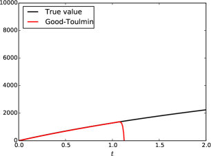
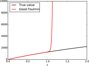
Figure 1: GT estimate as a function of $t$ for two realizations random samples of size $n=5000$ generated by a Zipf distribution $p_{i}\propto 1/(i+10)$ for $1\leq i\leq 10000$.

Naturally, we would like to estimate $U$ for as large a $t$ as possible. However, as $t>1$ increases, $U^{\scriptscriptstyle\rm GT}$ grows as $(-t)^{i}{\varPhi_{i}}$ for the largest $i$ such that ${\varPhi_{i}}>0$. Hence whenever any symbol appears more than once, $U^{\scriptscriptstyle\rm GT}$ grows super-linearly in $t$, eventually far exceeding $U$ that grows at most linearly in $t$. Figure 1 also shows that for the same Zipf distribution, for $t>1$ indeed $U^{\scriptscriptstyle\rm GT}$ does not approximate $U$ at all.

To predict $U$ for $t>1$, Good and Toulmin [GT56] suggested using the Euler transform [AS64] that converts an alternating series into another series with the same sum, and heuristically often converges faster. Interestingly, Efron and Thisted [ET76] showed that when the Euler transform of $U^{\scriptscriptstyle\rm GT}$ is truncated after $k$ terms, it can be expressed as another simple linear estimator,

$$U^{\scriptscriptstyle\rm ET}\stackrel{{\scriptstyle\mathrm{def}}}{{=}}\sum_{i=1}^{n}h^{\rm ET}_{i}\cdot{\varPhi_{i}},$$

where

$$h^{\rm ET}_{i}\stackrel{{\scriptstyle\mathrm{def}}}{{=}}-\left(-t\right)^{i}\cdot\mathbb{P}\left(\mathrm{Bin}\Big{(}k,\frac{1}{1+t}\Big{)}\geq i\right),$$

and

$$\mathbb{P}\left(\mathrm{Bin}\left(k,\frac{1}{1+t}\right)\geq i\right)=\begin{cases}\sum_{j=i}^{k}\binom{k}{j}\frac{t^{k-j}}{(1+t)^{k}}&i\leq k,\\ 0&i>k,\end{cases}$$

is the binomial tail probability that decays with $i$, thereby moderating the rapid growth of $(-t)^{i}$.

Over the years, $U^{\scriptscriptstyle\rm ET}$ has been used by numerous researchers in a variety of scenarios and a multitude of applications. Yet despite its wide-spread use and robust empirical results, no provable guarantees have been established for its performance or that of any related estimator when $t>1$. The lack of theoretical understanding, has also precluded clear guidelines for choosing the parameter $k$ in $U^{\scriptscriptstyle\rm ET}$.

2 Approach and results

We construct a family of estimators that provably predict $U$ optimally not just for constant $t>1$, but all the way up to $t\propto\log n$. This shows that per each observed sample, we can infer properties of $\log n$ yet unseen samples. The proof technique is general and provides a disciplined guideline for choosing the parameter $k$ for $U^{\scriptscriptstyle\rm ET}$ and, in addition, a modification that outperforms $U^{\scriptscriptstyle\rm ET}$.

2.1 Smoothed Good-Toulmin (SGT) estimator

To obtain a new class of estimators, we too start with $U^{\scriptscriptstyle\rm GT}$, but unlike $U^{\scriptscriptstyle\rm ET}$ that was derived from $U^{\scriptscriptstyle\rm GT}$ via analytical considerations aimed at improving the convergence rate, we take a probabilistic view that controls the bias and variance of $U^{\scriptscriptstyle\rm GT}$ and balances the two to obtain a more efficient estimator.

Note that what renders $U^{\scriptscriptstyle\rm GT}$ inaccurate when $t>1$ is not its bias but mainly its high variance due to the exponential growth of the coefficients $(-t)^{i}$ in (1); in fact $U^{\scriptscriptstyle\rm GT}$ is the unique unbiased estimator for all $t$ and $n$ in the closely related Poisson sampling model (see Section 3). Therefore it is tempting to truncate the series (1) at the $\ell^{\mathrm{th}}$ term and use the partial sum as an estimator:

$$U^{\ell}\stackrel{{\scriptstyle\mathrm{def}}}{{=}}-\sum_{i=1}^{\ell}\left(-t\right)^{i}{\varPhi_{i}}.$$ (2)

However, for $t>1$, it can be shown that for certain distributions most of the symbols typically appear $\ell$ times and hence the last term in (2) dominates, resulting in a large bias and inaccurate estimates regardless of the choice of $\ell$ (see Section 5.1 for a rigorous justification).

To resolve this problem, we truncate the Good-Toulmin estimator at a random location, denoted by an independent random nonnegative integer $L$, and average over the distribution of $L$, which yields the following estimator:

$$U^{\scriptscriptstyle\rm L}=\mathbb{E}_{L}\left[-\sum_{i=1}^{L}\left(-t\right)^{i}{\varPhi_{i}}\right].$$ (3)

The key insight is that since the bias of $U^{\ell}$ typically alternates signs as $\ell$ grows, averaging over different cutoff locations takes advantage of the cancellation and dramatically reduces the bias. Furthermore, the estimator (3) can be expressed simply as a linear combination of prevalences:

$$U^{\scriptscriptstyle\rm L}=\mathbb{E}_{L}\left[-\sum_{i\geq 1}\left(-t\right)^{i}{\varPhi_{i}}\mathbbm{1}_{i\leq L}\right]=-\sum_{i\geq 1}\left(-t\right)^{i}\mathbb{P}\left(L\geq i\right){\varPhi_{i}}.$$ (4)

We shall refer to estimators of the form (4) Smoothed Good-Toulmin (SGT) estimators and the distribution of $L$ the smoothing distribution.

Choosing different smoothing distributions results a variety of linear estimators, where the tail probability $\mathbb{P}\left(L\geq i\right)$ compensates the exponential growth of $\left(-t\right)^{i}$ thereby stabilizing the variance. Surprisingly, though the motivation and approach are quite different, SGT estimators include $U^{\scriptscriptstyle\rm ET}$ in (1) as a special case which corresponds to the binomial smoothing $L\sim\mathrm{Bin}(k,\frac{1}{1+t})$. This provides an intuitive probabilistic interpretation of $U^{\scriptscriptstyle\rm ET}$, which was originally derived via Euler’s transform and analytic considerations. As we show in the next section, this interpretation leads to the first theoretical guarantee for $U^{\scriptscriptstyle\rm ET}$ as well as improved estimators that are provably optimal.

2.2 Main results

Since $U$ takes in values between $0$ and $nt$, we measure the performance of an estimator $U^{\scriptscriptstyle\rm E}$ by the worst-case normalized mean-square error (NMSE),

$$\mathcal{E}_{n,t}(U^{\scriptscriptstyle\rm E})\stackrel{{\scriptstyle\mathrm{def}}}{{=}}\max_{p}\mathbb{E}_{p}\left(\frac{U^{\scriptscriptstyle\rm E}-U}{nt}\right)^{2}.$$

Observe that this criterion conservatively evaluates the performance of the estimator for the worst possible distribution. The trivial estimator that always predicts $nt/2$ new elements has NMSE equal to $1/4$, and we would like to construct estimators with vanishing NMSE, which can estimate $U$ up to an error that diminishes with $n$, regardless of the data-generating distribution; in particular, we are interested in the largest $t$ for which this is possible.

Relating the bias and variance of $U^{\scriptscriptstyle\rm L}$ to the expectation of $t^{L}$ and another functional we obtain the following performance guarantee for SGT estimators with appropriately chosen smoothing distributions.

Theorem 1.

For Poisson or binomially distributed $L$ with the parameters given in Table 1, for all $t\geq 1$ and $n\in\mathbb{N}$,

$$\mathcal{E}_{n,t}(U^{\scriptscriptstyle\rm L})\lesssim\frac{1}{n^{1/t}}.$$

Smoothing distribution	Parameters	$\mathcal{E}_{n,t}(U^{\scriptscriptstyle\rm L})\lesssim$
Poisson $(r)$	$r=\frac{1}{2t}\log_{e}\frac{n(t+1)^{2}}{t-1}$	$n^{-1/t}$
Binomial $(k,q)$	$k=\left\lceil\frac{1}{2}\log_{2}\frac{nt^{2}}{t-1}\right\rceil$, $q=\frac{1}{t+1}$	$n^{-\log_{2}(1+1/t)}$
Binomial $(k,q)$	$k=\left\lceil\frac{1}{2}\log_{3}\frac{nt^{2}}{t-1}\right\rceil$, $q=\frac{2}{t+2}$	$n^{-\log_{3}(1+2/t)}$

Table 1: NMSE of SGT estimators for three smoothing distributions. Since for any $t\geq 1$, $\log_{3}(1+2/t)\geq\log_{2}(1+1/t)\geq 1/t$, binomial smoothing with $q=2/(2+t)$ yields the best convergence rate.

Theorem 1 provides a principled way for choosing the parameter $k$ for $U^{\scriptscriptstyle\rm ET}$ and the first provable guarantee for its performance, shown in Table 1. Furthermore, the result shows that a modification of $U^{\scriptscriptstyle\rm ET}$ with $q=\frac{2}{t+2}$ enjoys even faster convergence rate and, as experimentally demonstrated in Section 8, outperforms the original version of Efron-Thisted as well as other state-of-the-art estimators.

Furthermore, SGT estimators are essentially optimal as witnessed by the following matching minimax lower bound.

Theorem 2.

There exist universal constant $c,c^{\prime}$ such that for any $t\geq c$, any $n\in\mathbb{N}$, and any estimator $U^{\scriptscriptstyle\rm E}$

$$\mathcal{E}_{n,t}(U^{\scriptscriptstyle\rm E})\gtrsim\frac{1}{n^{c^{\prime}/t}}.$$

Theorems 1 and 2 determine the limit of predictability up to a constant multiple.

Corollary 1.

For any $\delta>0$,

$$\lim_{n\to\infty}\frac{\max\{t:\mathcal{E}_{n,t}(U^{\scriptscriptstyle\rm E})<\delta\textrm{\,\, for some $U^{\scriptscriptstyle\rm E}$}\}}{\log n}\asymp\frac{1}{\log\frac{1}{\delta}}.$$

The rest of the paper is organized as follows: In Section 3, we describe the four statistical models commonly used across various scientific disciplines, namely, the multinomial, Poisson, hypergeometric, and Bernoulli product models. Among the four models Poisson is the simplest to analyze and hence in Sections 4 and 5, we first prove Theorem 1 for the Poisson model and in Section 6 we prove similar results for the other three statistical models. In Section 7, we prove the lower bound for the multinomial and Poisson models. Finally, in Section 8 we demonstrate the efficiency and practicality of our estimators on a variety of synthetic and data sets.

3 Statistical models

The extrapolation paradigm has been applied to several statistical models. In all of them, an initial sample of size related to $n$ is collected, resulting in a set $S_{\text{old}}$ of observed elements. We consider collecting a new sample of size related to $m$, that would result in a yet unknown set $S_{\text{new}}$ of observed elements, and we would like to estimate

$$|S_{\text{new}}\backslash S_{\text{old}}|,$$

the number of unseen symbols that will appear in the new sample. For example, for the observed sample bananas and future sample sonatas, $S_{\text{old}}=\{\tt a,b,n,s\}$, $S_{\text{new}}=\{\tt a,n,o,s,t\}$, and $|S_{\text{new}}\backslash S_{\text{old}}|=|\{\tt o,t\}|=2$.

Four statistical models have been commonly used in the literature (cf. survey [BF93] and [CCG⁺12]), and our results apply to all of them. The first three statistical models are also referred as the abundance models and the last one is often referred to as the incidence model in ecology [CCG⁺12].

Multinomial:

This is Good and Toulmin’s original model where the samples are independently and identically distributed (i.i.d.), and the initial and new samples consist of exactly $n$ and $m$ elements respectively. Formally, $X^{n+m}=X_{1},\ldots,X_{n+m}$ are generated independently according to an unknown discrete distribution of finite or even infinite support, $S_{\text{old}}=\{X^{n}\}$, and $S_{\text{new}}=\{X_{n+1}^{n+m}\}$.

Hypergeometric:

This model corresponds to a sampling-without-replacement variant of the multinomial model. Specifically, $X^{n+m}$ are drawn uniformly without replacement from an unknown collection of symbols that may contain repetitions, for example, an urn with some white and black balls. Again, $S_{\text{old}}=\{X^{n}\}$ and $S_{\text{new}}=\{X_{n+1}^{n+m}\}$.

Poisson:

As in the multinomial model, the samples are also i.i.d., but the sample sizes, instead of being fixed, are Poisson distributed. Formally, $N\sim\mathrm{poi}(n)$, $M\sim\mathrm{poi}(m)$, $X^{N+M}$ are generated independently according to an unknown discrete distribution, $S_{\text{old}}=\{X^{N}\}$, and $S_{\text{new}}=\{X_{N+1}^{N+M}\}$.

Bernoulli-product:

In this model we observe signals from a collection of independent processes over subset of an unknown set $\mathcal{X}$. Every $x\in\mathcal{X}$ is associated with an unknown probability $0\leq p_{x}\leq 1$, where the probabilities do not necessarily sum to 1. Each sample $X_{i}$ is a subset of $\mathcal{X}$ where symbol $x\in\mathcal{X}$ appears with probability $p_{x}$ and is absent with probability $1-p_{x}$, independently of all other symbols. $S_{\text{old}}=\cup_{i=1}^{n}X_{i}$ and $S_{\text{new}}=\cup_{i=n+1}^{n+m}X_{i}$.

For theoretical analysis in Sections 4 and 5 we use the Poisson sampling model as the leading example due to its simplicity. Later in Section 6, we show that very similar results continue to hold for the other three models.

We close this section by discussing two problems that are closely related to the extrapolation model, namely, support size estimation and missing mass estimation, which correspond to $m=\infty$ and $m=1$ respectively. Indeed, the probability that the next sample is new is precisely the expected value of $U$ for $m=1$, which is the goal in the basic Good-Turing problem [Goo53, Rob68, MS00, OS15]. On the other hand, any estimator $U^{\scriptscriptstyle\rm E}$ for $U$ can be converted to a (not necessarily good) support size estimator by adding the number of observed symbols. Estimating the support size of an underlying distribution has been studied by both ecologists [Cha84, CL92, BF93] and theoreticians [RRSS09, VV11, VV13, WY15b]; however, to make the problem non-trivial, all statistical models impose a lower bound on the minimum non-zero probability of each symbol, which is assumed to be known to the statistician. We discuss these estimators and their differences to our results in Section 4.3.

4 Preliminaries and the Poisson model

Throughout the paper, we use standard asymptotic notation, e.g., for any positive sequences $\{a_{n}\}$ and $\{b_{n}\}$, denote $a_{n}=\Theta(b_{n})$ or $a_{n}\asymp b_{n}$ if $1/c\leq a_{n}/b_{n}\leq c$ for some universal constant $c>0$. Let $\mathbbm{1}_{A}$ denote the indicator random variable of an event $A$. Let $\mathrm{Bin}(n,p)$ denote the binomial distribution with $n$ trials and success probability $p$ and let $\mathrm{poi}(\lambda)$ denote the Poisson distribution with mean $\lambda$. All logarithms are with respect to the natural base unless otherwise specified.

Let $p$ be a probability distribution over a discrete set $\mathcal{X}$, namely $p_{x}\geq 0$ for all $x\in\mathcal{X}$ and $\sum_{x\in\mathcal{X}}p_{x}=1$. Recall that the sample sizes are Poisson distributed: $N\sim\mathrm{poi}(n)$, $M\sim\mathrm{poi}(m)$, and $t=\frac{m}{n}$. We abbreviate the number of unseen symbols by

$$U\stackrel{{\scriptstyle\mathrm{def}}}{{=}}U(X^{N},X_{N+1}^{N+M}),$$

and we denote an estimator by $U^{\scriptscriptstyle\rm E}\stackrel{{\scriptstyle\mathrm{def}}}{{=}}U^{\scriptscriptstyle\rm E}(X^{N},t)$.

Let $N_{x}$ and $N_{x}^{\prime}$ denote the multiplicity of a symbol $x$ in the current samples and future samples, respectively. Let $\lambda_{x}\stackrel{{\scriptstyle\mathrm{def}}}{{=}}np_{x}$. Then a symbol $x$ appears $N_{x}\sim\mathrm{poi}(np_{x})=\mathrm{poi}(\lambda_{x})$ times, and for any $i\geq 0$,

$$\mathbb{E}[\mathbbm{1}_{N_{x}=i}]=e^{-\lambda_{x}}\frac{\lambda_{x}^{i}}{i!}.$$

Hence

$$\mathbb{E}[{\varPhi_{i}}]=\mathbb{E}\left[\sum_{x}\mathbbm{1}_{N_{x}=i}\right]=\sum_{x}e^{-\lambda_{x}}\frac{\lambda_{x}^{i}}{i!}.$$

A helpful property of Poisson sampling is that the multiplicities of different symbols are independent of each other. Therefore, for any function $f(x,i)$,

$$\mathrm{Var}\left(\sum_{x}f(x,N_{x})\right)=\sum_{x}\mathrm{Var}(f(x,N_{x})).$$

Many of our derivations rely on these three equations. For example,

$$\mathbb{E}[U]=\sum_{x}\mathbb{E}[\mathbbm{1}_{N_{x}=0}]\cdot\mathbb{E}[\mathbbm{1}_{N_{x}^{\prime}>0}]=\sum_{x}e^{-\lambda_{x}}\cdot(1-e^{-t\lambda_{x}}),$$

and

$$\mathrm{Var}(U) =\mathrm{Var}\left(\sum_{x}\mathbbm{1}_{N_{x}=0}\cdot\mathbbm{1}_{N_{x}^{\prime}>0}\right)=\sum_{x}\mathrm{Var}\left(\mathbbm{1}_{N_{x}=0}\cdot\mathbbm{1}_{N_{x}^{\prime}>0}\right)$$

$$\leq\sum_{x}\mathbb{E}\left[\mathbbm{1}_{N_{x}=0}\cdot\mathbbm{1}_{N_{x}^{\prime}>0}\right]=\mathbb{E}\left[U\right].$$

Note that these equations imply that the standard deviation of $U$ is at most $\sqrt{\mathbb{E}[U]}\ll\mathbb{E}[U]$, hence $U$ highly concentrates around its expectation, and estimating $U$ and $\mathbb{E}[U]$ are essentially the same.

4.1 The Good-Toulmin estimator

Before proceeding with general estimators, we prove a few properties of $U^{\scriptscriptstyle\rm GT}$. Under the Poisson model, $U^{\scriptscriptstyle\rm GT}$ is in fact the unique unbiased estimator for $U$.

Lemma 1 ([ET76]).

For any distribution,

$$\mathbb{E}[U]=\mathbb{E}[U^{\scriptscriptstyle\rm GT}].$$

Proof.

$$\mathbb{E}[U] =\mathbb{E}\left[\sum_{x}\mathbbm{1}_{N_{x}=0}\cdot\mathbbm{1}_{N_{x}>0}\right]=\sum_{x}e^{-\lambda_{x}}\cdot\left(1-e^{-t\lambda_{x}}\right)$$

$$=-\sum_{x}e^{-\lambda_{x}}\cdot\sum^{\infty}_{i=1}\frac{(-t\lambda_{x})^{i}}{i!}=-\sum^{\infty}_{i=1}(-t)^{i}\cdot\sum_{x}e^{-\lambda_{x}}\frac{\lambda_{x}^{i}}{i!}$$

$$=-\sum^{\infty}_{i=1}(-t)^{i}\cdot\mathbb{E}[{\varPhi_{i}}]=\mathbb{E}[U^{\scriptscriptstyle\rm GT}].\qed$$

Even though $U^{\scriptscriptstyle\rm GT}$ is unbiased for all $t$, for $t>1$ it has high variance and hence does not estimate $U$ well even for the simplest distributions.

Lemma 2.

For any $t>1$,

$$\lim_{n\to\infty}\mathcal{E}_{n,t}(U^{\scriptscriptstyle\rm GT})=\infty.$$

Proof.

Let $p$ be the uniform distribution over two symbols $a$ and $b$, namely, $p_{a}=p_{b}=1/2$. First consider even $n$. Since $(U^{\scriptscriptstyle\rm GT}-U)^{2}$ is always nonnegative,

$$\mathbb{E}[(U^{\scriptscriptstyle\rm GT}-U)^{2}]\geq\mathbb{P}(N_{a}=N_{b}=n/2)(2(-t)^{n/2})^{2}=\left(e^{-n/2}\frac{(n/2)^{n/2}}{(n/2)!}\right)^{2}4t^{n}\geq\frac{4t^{n}}{e^{2}n},$$

where we used the fact that $k!\leq(\frac{k}{e})^{k}\sqrt{k}e$. Hence for $t>1$,

$$\lim_{n\to\infty}\frac{\mathbb{E}[(U^{\scriptscriptstyle\rm GT}-U)^{2}]}{(nt)^{2}}\geq\lim_{n\to\infty}\frac{4t^{n}}{e^{2}n(nt)^{2}}=\infty.$$

The case of odd $n$ can be shown similarly by considering the event $N_{a}=\lfloor n/2\rfloor,N_{b}=\lceil n/2\rceil$. ∎

4.2 General linear estimators

Following [ET76], we consider general linear estimators of the form

$$U^{\scriptscriptstyle\rm h}=\sum^{\infty}_{i=1}{\varPhi_{i}}\cdot h_{i},$$ (5)

which can be identified with a formal power series $h(y)=\sum^{\infty}_{i=1}\frac{h_{i}y^{i}}{i!}$. For example, $U^{\scriptscriptstyle\rm GT}$ in (1) corresponds to the function $h(y)=1-e^{-yt}$. The next lemma bounds the bias and variance of any linear estimator $U^{\scriptscriptstyle\rm h}$ using properties of the function $h$. In Section 5.2 we apply this result to the SGT estimator whose coefficients are of the specific form:

$$h_{i}=-\left(-t\right)^{i}\cdot\mathbb{P}\left(L\geq i\right).$$

Let ${\varPhi_{+}}\stackrel{{\scriptstyle\mathrm{def}}}{{=}}\sum^{\infty}_{i=1}{\varPhi_{i}}$ denote the number of observed symbols.

Lemma 3.

The bias of $U^{\scriptscriptstyle\rm h}$ is

$$\mathbb{E}[U^{\scriptscriptstyle\rm h}-U]=\sum_{x}e^{-\lambda_{x}}\left(h(\lambda_{x})-(1-e^{-t\lambda_{x}})\right),$$

and the variance satisfies

$$\mathrm{Var}(U^{\scriptscriptstyle\rm h}-U)\leq\mathbb{E}[{\varPhi_{+}}]\cdot\sup_{i\geq 1}h^{2}_{i}+\mathbb{E}[U].$$

Proof.

Note that

$$U^{\scriptscriptstyle\rm h}-U =\sum^{\infty}_{i=1}{\varPhi_{i}}h_{i}-\sum_{x}\mathbbm{1}_{N_{x}=0}\cdot\mathbbm{1}_{N_{x}^{\prime}>0}$$

$$=\sum^{\infty}_{i=1}\sum_{x}\mathbbm{1}_{N_{x}=i}\cdot h_{i}-\sum_{x}\mathbbm{1}_{N_{x}=0}\cdot\mathbbm{1}_{N_{x}^{\prime}>0}$$

$$=\sum_{x}\left(\sum^{\infty}_{i=1}\mathbbm{1}_{N_{x}=i}\cdot h_{i}-\mathbbm{1}_{N_{x}=0}\cdot\mathbbm{1}_{N_{x}^{\prime}>0}\right).$$

For every symbol $x$,

$$\mathbb{E}\left[\sum^{\infty}_{i=1}\mathbbm{1}_{N_{x}=i}\cdot h_{i}-\mathbbm{1}_{N_{x}=0}\cdot\mathbbm{1}_{N_{x}^{\prime}>0}\right] =\sum^{\infty}_{i=1}e^{-\lambda_{x}}\frac{\lambda^{i}_{x}}{i!}\cdot h_{i}-e^{-\lambda_{x}}\cdot(1-e^{-t\lambda_{x}})$$

$$=e^{-\lambda_{x}}\left(\sum^{\infty}_{i=1}\frac{\lambda^{i}_{x}h_{i}}{i!}-(1-e^{-t\lambda_{x}})\right)$$

$$=e^{-\lambda_{x}}\left(h(\lambda_{x})-(1-e^{-t\lambda_{x}})\right),$$

from which (3) follows. For the variance, observe that for every symbol $x$,

$$\mathrm{Var}\left(\sum^{\infty}_{i=1}\mathbbm{1}_{N_{x}=i}\cdot h_{i}-\mathbbm{1}_{N_{x}=0}\cdot\mathbbm{1}_{N_{x}^{\prime}>0}\right) \leq\mathbb{E}\left[\left(\sum^{\infty}_{i=1}\mathbbm{1}_{N_{x}=i}\cdot h_{i}-\mathbbm{1}_{N_{x}=0}\cdot\mathbbm{1}_{N_{x}^{\prime}>0}\right)^{2}\right]$$

$$\stackrel{{\scriptstyle(a)}}{{=}}\mathbb{E}\left[\sum^{\infty}_{i=1}\mathbbm{1}_{N_{x}=i}h_{i}^{2}\right]+\mathbb{E}[\mathbbm{1}_{N_{x}=0}]\cdot\mathbb{E}[\mathbbm{1}_{N_{x}^{\prime}>0}]$$

$$=\sum^{\infty}_{i=1}\mathbb{E}[\mathbbm{1}_{N_{x}=i}]\cdot h_{i}^{2}+\mathbb{E}[\mathbbm{1}_{N_{x}=0}]\cdot\mathbb{E}[\mathbbm{1}_{N_{x}^{\prime}>0}],$$

where $(a)$ follows as for every $i\neq j$, $\mathbb{E}[\mathbbm{1}_{N_{x}=i}\mathbbm{1}_{N_{x}=j}]=0$. Since the variance of a sum of independent random variables is the sum of variances,

$$\mathrm{Var}(U^{\scriptscriptstyle\rm h}-U) \leq\sum_{x}\sum^{\infty}_{i=1}\mathbb{E}[\mathbbm{1}_{N_{x}=i}]h_{i}^{2}+\sum_{x}\mathbb{E}[\mathbbm{1}_{N_{x}=0}]\cdot\mathbb{E}[\mathbbm{1}_{N_{x}^{\prime}>0}]$$

$$=\sum^{\infty}_{i=1}\mathbb{E}[{\varPhi_{i}}]\cdot h_{i}^{2}+\mathbb{E}[U]$$

$$\leq\mathbb{E}[{\varPhi_{+}}]\cdot\sup_{i\geq 1}h^{2}_{i}+\mathbb{E}[U].\qed$$

Lemma 3 enables us to reduce the estimation problem to a task on approximating functions. Specifically, in view of (3), the goal is to approximate $1-e^{-yt}$ by a function $h(y)$ whose derivatives at zero all have small magnitude.

4.3 Estimation via polynomial approximation and support size estimation

Approximation-theoretic techniques for estimating norms and other properties such as support size and entropy have been successfully used in the statistics literature. For example, estimating the $L_{p}$ norms in Gaussian models [LNS99, CL11] and estimating entropy [WY15b, JVHW15] and support size [WY15a] of discrete distributions. Among the aforementioned problems, support size estimation is closest to ours. Hence, we now discuss the difference between the approximation technique we use and the those used for support size estimation.

The support size of a discrete distribution $p$ is

$$S(p)=\sum_{x}\mathbbm{1}_{p_{x}>0}.$$ (6)

At the first glance, estimating $S(p)$ may appear similar to species estimation problem as one can convert a support size estimator $\hat{S}$ to $\hat{U}$ by

$$\hat{U}=\hat{S}-\sum^{\infty}_{i=1}{\varPhi_{i}}.$$

However, without any assumption on the distribution it is impossible to estimate the support size. For example, regardless how many samples are collected, there could be infinitely many symbols with arbitrarily small probabilities that will never be observed. A common assumption is therefore that the minimum non-zero probability of the underlying distribution $p$, denoted by $p^{+}_{\min}$, is at least $1/k$, for some known $k$. Under this assumption [VV11] used a linear programming estimator similar to the one in [ET76], to estimate the support size within an additive error of $k\epsilon$ with constant probability using $\Omega(\frac{k}{\log k}\frac{1}{\epsilon^{2}})$ samples. Based on best polynomial approximations recently [WY15a] showed that the minimax risk of support size estimation satisfies

$$\min_{\hat{S}}\max_{p:p^{+}_{\min}\geq 1/k}\mathbb{E}_{p}[(\hat{S}-S(p))^{2}]=k^{2}\exp\left(-\Theta\left(\max\left\{\sqrt{\frac{k\log k}{n}},\frac{k}{n},1\right\}\right)\right)$$

and that the optimal sample complexity of for estimating $S(p)$ within an additive error of $k\epsilon$ with constant probability is in fact $\Theta(\frac{k}{\log k}\log^{2}\frac{1}{\epsilon})$. Note that the assumption $p^{+}_{\min}\geq 1/k$ is crucial for this result to hold for otherwise estimation is impossible; in contrast, as we show later, for species estimation no such assumptions are necessary. The intuition is that if there exist a large number of very improbable symbols, most likely they will not appear in the new samples anyway.

To estimate the support size, in view of (6) and the assumption $p^{+}_{\min}\geq 1/k$, the technique of [WY15a] is to approximate the indicator function $y\mapsto\mathbbm{1}_{y\geq 1/k}$ in the range $\{0\}\cup[1/k,\log k/n]$ using Chebyshev polynomials. Since by assumption no $p_{x}$ lies in $(0,\frac{1}{k})$, the approximation error in this interval is irrelevant. For example, in Figure 2, the red curve is a useful approximation for the support size, even though it behaves badly over $(0,1/k)$. To estimate the average number of unseen symbols $U$, in view of (3), we need to approximate $y\mapsto 1-e^{-yt}$ over the entire $[0,\infty)$ as in, e.g., Figure 2.

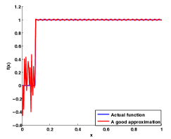
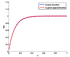
Figure 2: (a) a good approximation for support size; (b) a good approximation for species estimation.

Concurrent to this work, [VV15] proposed a linear programming algorithm to estimate $U$. However, their NMSE is $O(\frac{t}{\log n})$ compared to the optimal result $O(n^{-1/t})$ in Theorem 1, thus exponentially weaker for $t=o(\log n)$. Furthermore, the computational cost far exceeds those of our linear estimators.

5 Results for the Poisson model

In this section, we provide the performance guarantee for SGT estimators under the Poisson sampling model. We first show that the truncated GT estimators incurs a high bias. We then introduce the class of smoothed GT estimators obtained by averaging several truncated GT estimators and bound their mean squared error in Theorem 3 for an arbitrary smoothing distribution. We then apply this result to obtain NMSE bounds for Poisson and Binomial smoothing in Corollaries 2 and 3 respectively, which imply the main result (Theorem 1) announced in Section 2.2 for the Poisson model.

5.1 Why truncated Good-Toulmin does not work

Before we discuss the SGT estimator, we first show that the naive approach of truncating the GT estimator described in Section 2.1 leads to bad performance when $t>1$. Recall from Lemma 3 that designing a good linear estimator boils to approximating $1-e^{-yt}$ by an analytic function $h(y)=\sum_{i\geq 1}\frac{h_{i}}{i!}y^{i}$ such that all its derivatives at zero are small, namely, $\sup_{i\geq 1}|h_{i}|$ is small. The GT estimator corresponds to the perfect approximation

$$h^{\scriptscriptstyle\rm GT}(y)=1-e^{-yt};$$

however, $\sup_{i\geq 1}|h_{i}|=\max(t,t^{\infty})$, which is infinity if $t>1$ and leads to large variance. To avoid this situation, a natural approach is to use use the $\ell$-term Taylor expansion of $1-e^{-yt}$ at $0$, namely,

$$h^{\ell}(y)=-\sum^{\ell}_{i=1}\frac{(-yt)^{i}}{i!},$$ (7)

which corresponds to the estimator $U^{\ell}$ defined in (2). Then $\sup_{i\geq 1}|h_{i}|=t^{\ell}$ and, by Lemma 3, the variance is at most $n(t^{\ell}+t)$. Hence if ${\ell}\leq\log_{t}m$, the variance is at most $n(m+t)$. However, note that the $\ell$-term Taylor approximation is a degree-$\ell$ polynomial which eventually diverges and deviates from $1-e^{-yt}$ as $y$ increases, thereby incurring a large bias. Figure 3 illustrates this phenomenon by plotting the function $1-e^{-yt}$ and its Taylor expansion with $5,10,$ and $20$ terms.

.

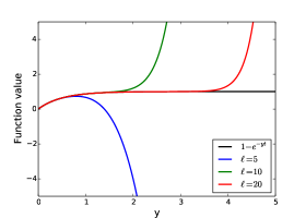
Figure 3: (a) Taylor approximation for $t=2$, (b) Averages of $10$ and $11$ term Taylor approximation $t=2$.

Indeed, the next result (proved in Appendix A) rigorously shows that the NMSE of truncated GT estimator never vanishes:

Lemma 4.

There exist a constant $c>0$ such that for any $\ell\geq 0$, any $t>1$ and any $n\in\mathbb{N}$,

$$\mathcal{E}_{n,t}(U^{\scriptscriptstyle\ell})\geq\frac{c(t-1)^{5}}{t^{4}}.$$

5.2 Smoothing by random truncation

As we saw in the previous section, the $\ell$-term Taylor approximation, where all the coefficients after the $\ell^{\mathrm{th}}$ term are set to zero results in large bias. Instead, one can choose a weighted average of several Taylor series approximations, whose biases cancel each other leading to significant bias reduction. For example, in Figure 3, we plot

$$wh^{10}+(1-w)h^{11}$$

for various values of $w\in[0,1]$. Notice that the weight $w=0.6$ leads to better approximation of $1-e^{-yt}$ than both $h^{10}$ and $h^{11}$.

A natural generalization of the above argument entails taking the weighted average of various Taylor approximations with respect to a given probability distribution over $\mathbb{Z}_{+}\stackrel{{\scriptstyle\mathrm{def}}}{{=}}\{0,1,2,\ldots\}$. For a $\mathbb{Z}_{+}$-valued random variable $L$, consider the power series

$$h^{\scriptscriptstyle\rm L}(y)=\sum^{\infty}_{\ell=0}\mathbb{P}(L=\ell)\cdot h^{\ell}(y),$$

where $h^{\ell}$ is defined in (7). Rearranging terms, we have

$$h^{\scriptscriptstyle\rm L}(y)=\sum^{\infty}_{\ell=0}\mathbb{P}(L=\ell)\sum^{\ell}_{i=1}\frac{-(-yt)^{i}}{i!}=-\sum^{\infty}_{i=1}\frac{(-yt)^{i}}{i!}\mathbb{P}(L\geq i).$$

Thus, the linear estimator with coefficients

$$h^{\scriptscriptstyle\rm L}_{i}=-(-t)^{i}\mathbb{P}\left(L\geq i\right),$$ (8)

is precisely the SGT estimator $U^{\scriptscriptstyle\rm L}$ defined in (4). Special cases of smoothing distributions include:

• $L=\infty$: This corresponds to the original Good-Toulmin estimator (1) without smoothing;

• $L=\ell$ deterministically: This leads to the estimator $U^{\ell}$ in (2) corresponding to the $\ell$-term Taylor approximation;

• $L\sim\mathrm{Bin}(k,1/(1+t))$: This recovers the Efron-Thisted estimator (1), where $k$ is a tuning parameter to be chosen.

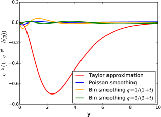
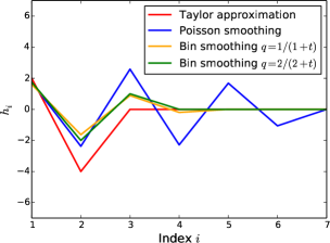
Figure 4: Comparisons of approximations of $h^{\scriptscriptstyle\rm L}(\cdot)$ with $\mathbb{E}[L]=2$ and $t=2$. (a) $e^{-y}(1-e^{-yt}-h^{\scriptscriptstyle\rm L}(y))$ as a function of $y$. (b) Coefficients $h^{\scriptscriptstyle\rm L}_{i}$ as a function of index $i$.

We study the performance of linear estimators corresponding to the Poisson smoothing and the Binomial smoothing. To this end, we first systematically upper bound the bias and variance for any probability smoothing $L$. We plot the error that corresponds to each smoothing in Figure 4. Notice that the Poisson and binomial smoothings have significantly small error compared to the Taylor series approximation. The coefficients of the resulting estimator is plotted in Figure 4. It is easy so see that the maximum absolute value of the coefficient is higher for the Taylor series approximation compared to the Poisson or binomial smoothings.

Lemma 5.

For a random variable $L$ over $\mathbb{Z}_{+}$ and $t\geq 1$,

$$\mathrm{Var}(U^{\scriptscriptstyle\rm L}-U)\leq\mathbb{E}[{\varPhi_{+}}]\cdot{\mathbb{E}}^{2}[t^{L}]+\mathbb{E}[U].$$

Proof.

By Lemma 3, to bound the variance it suffices to bound the highest coefficient in $h^{\scriptscriptstyle\rm L}$.

$$|h^{\scriptscriptstyle\rm L}_{i}|\leq t^{i}\mathbb{P}(L\geq i)=t^{i}\sum^{\infty}_{j=i}\mathbb{P}(L=j)\leq\sum^{\infty}_{j=i}\mathbb{P}(L=j)t^{j}\leq\mathbb{E}[t^{L}].$$ (9)

The above bound together with Lemma 3 yields the result. ∎

To bound the bias, we need few definitions. Let

$$g(y)\stackrel{{\scriptstyle\mathrm{def}}}{{=}}-\sum_{i=1}^{\infty}\frac{\mathbb{P}\left(L\geq i\right)}{i!}(-y)^{i}.$$ (10)

Under this definition, $h^{\scriptscriptstyle\rm L}(y)=g(yt)$. We use the following auxiliary lemma to bound the bias.

Lemma 6.

For any random variable $L$ over $\mathbb{Z}_{+}$,

$$g(y)-(1-e^{-y})=-e^{-y}\int_{0}^{y}\mathbb{E}\left[{\frac{(-s)^{L}}{L!}}\right]e^{s}\text{d}s.$$

Proof.

Subtracting (10) from the Taylor series expansion of $1-e^{-y}$ ,

$$g(y)-(1-e^{-y})= ~{}\sum_{i=1}^{\infty}\frac{\mathbb{P}\left(L<i\right)}{i!}(-y)^{i}$$

$$= ~{}\sum_{i=1}^{\infty}\sum_{j=0}^{i-1}\frac{(-y)^{i}}{i!}\mathbb{P}\left(L=j\right)$$

$$= ~{}\sum_{j=0}^{\infty}\left(\sum_{i=j+1}^{\infty}\frac{(-y)^{i}}{i!}\right)\mathbb{P}\left(L=j\right).$$

Note that $\sum_{i=j+1}^{\infty}\frac{z^{i}}{i!}$ can be expressed (via incomplete Gamma function) as

$$\sum_{i=j+1}^{\infty}\frac{z^{i}}{i!}=\frac{e^{z}}{j!}\int_{0}^{z}\tau^{j}e^{-\tau}\text{d}\tau.$$

Thus by Fubini’s theorem,

$$g(y)-(1-e^{-y})= ~{}\sum_{j=0}^{\infty}\frac{e^{-y}}{j!}\int_{0}^{-y}\tau^{j}e^{-\tau}\text{d}\tau\mathbb{P}\left(L=j\right)$$

$$= ~{}e^{-y}\int_{0}^{-y}e^{-\tau}\text{d}\tau\left(\sum_{j=0}^{\infty}\frac{\tau^{j}}{j!}\mathbb{P}\left(L=j\right)\right)$$

$$= ~{}-e^{-y}\int_{0}^{y}e^{s}\text{d}s\left(\sum_{j=0}^{\infty}\frac{(-s)^{j}}{j!}\mathbb{P}\left(L=j\right)\right)$$

$$= ~{}-e^{-y}\int_{0}^{y}\mathbb{E}\left[{\frac{(-s)^{L}}{L!}}\right]e^{s}\text{d}s.\qed$$

To bound the bias, we need one more definition. For a random variable $L$ over $\mathbb{Z}_{+}$, let

$$\xi_{L}(t)\stackrel{{\scriptstyle\mathrm{def}}}{{=}}\max_{0\leq s<\infty}\left\lvert\mathbb{E}\left[{\frac{(-s)^{L}}{L!}}\right]\right\rvert e^{-s/t},$$

Lemma 7.

For a random variable $L$ over $\mathbb{Z}_{+}$,

$$|\mathbb{E}[U^{\scriptscriptstyle\rm L}-U]|\leq(\mathbb{E}[{\varPhi_{+}}]+\mathbb{E}[U])\cdot\xi_{L}(t).$$

Proof.

By Lemma 6,

$$|g(y)-(1-e^{-y})| \leq e^{-y}\int_{0}^{y}\left\lvert\mathbb{E}\left[{\frac{(-s)^{L}}{L!}}\right]\right\rvert e^{s}\text{d}s$$

$$\leq\max_{s\leq y}\left\lvert\mathbb{E}\left[{\frac{(-s)^{L}}{L!}}\right]\right\rvert e^{-y}\int_{0}^{y}e^{s}\text{d}s$$

$$=\max_{s\leq y}\left\lvert\mathbb{E}\left[{\frac{(-s)^{L}}{L!}}\right]\right\rvert(1-e^{-y}).$$

For a symbol $x$,

$$e^{-\lambda_{x}}\left(h^{\scriptscriptstyle\rm L}(\lambda_{x})-(1-e^{-\lambda_{x}t})\right)=e^{-\lambda_{x}}\left(g(\lambda_{x}t)-(1-e^{-\lambda_{x}t})\right).$$

Hence,

$$\lvert e^{-\lambda_{x}}\left(h^{\scriptscriptstyle\rm L}(\lambda_{x})-1-e^{-\lambda_{x}t}\right)\rvert \leq(1-e^{-\lambda_{x}t})\max_{0\leq y\leq\infty}e^{-y}\max_{0\leq s\leq yt}\left\lvert\mathbb{E}\left[{\frac{(-s)^{L}}{L!}}\right]\right\rvert$$

$$\leq(1-e^{-\lambda_{x}t})\max_{0\leq s\leq\infty}\left\lvert\mathbb{E}\left[{\frac{(-s)^{L}}{L!}}\right]\right\rvert e^{-s/t}.$$

The lemma follows by summing over all the symbols and substituting $\sum_{x}1-e^{-\lambda_{x}t}\leq\sum_{x}1-e^{-\lambda_{x}(t+1)}=\mathbb{E}[{\varPhi_{+}}]+\mathbb{E}[U]$. ∎

The above two lemmas yield our main result.

Theorem 3.

For any random variable $L$ over $\mathbb{Z}_{+}$ and $t\geq 1$,

$$\mathbb{E}[(U^{\scriptscriptstyle\rm L}-U)^{2}]\leq\mathbb{E}[{\varPhi_{+}}]\cdot{\mathbb{E}}^{2}[t^{L}]+\mathbb{E}[U]+(\mathbb{E}[{\varPhi_{+}}]+\mathbb{E}[U])^{2}\xi_{L}(t)^{2}.$$

We have therefore reduced the problem of computing mean-squared loss, to that of computing expectation of certain function of the random variable. We now apply the above theorem for Binomial and Poisson smoothings. Notice that the above bound is distribution dependent and can be used to obtain stronger results for certain distributions. However, in the rest of the paper, we concentrate on obtaining minimax guarantees.

5.3 Poisson smoothing

Corollary 2.

For $t\geq 1$, $L\sim\mathrm{poi}(r)$ with $r=\frac{1}{2t}\log\left(\frac{n(t+1)^{2}}{t-1}\right)$,

$$\mathcal{E}_{n,t}(U^{\scriptscriptstyle\rm L})\leq\frac{c_{t}}{n^{1/t}},$$

where $0\leq c_{t}\leq 3$ and $\lim_{t\to\infty}c_{t}=1$.

Proof.

For $L\sim\mathrm{poi}(r)$,

$$\mathbb{E}[t^{L}]=e^{-r}\sum^{\infty}_{\ell=0}\frac{(rt)^{\ell}}{\ell!}=e^{r(t-1)}.$$ (11)

Furthermore,

$$\mathbb{E}\left[{\frac{(-s)^{L}}{L!}}\right]=e^{-r}\sum_{j=0}^{\infty}\frac{(-sr)^{j}}{(j!)^{2}}=e^{-r}J_{0}(2\sqrt{sr}),$$

where $J_{0}$ is the Bessel function of first order which takes values in $[-1,1]$ cf. [AS64, 9.1.60]. Therefore

$$\xi_{L}(t)\leq e^{-r}.$$ (12)

Equations (11) and (12) together with Theorem 3 yields

$$\mathbb{E}[(U^{\scriptscriptstyle\rm L}-U)^{2}]\leq\mathbb{E}[{\varPhi_{+}}]\cdot e^{2r(t-1)}+\mathbb{E}[U]+(\mathbb{E}[{\varPhi_{+}}]+\mathbb{E}[U])^{2}\cdot e^{-2r}.$$

Since $\mathbb{E}[{\varPhi_{+}}]\leq n$ and $\mathbb{E}[U]\leq nt$,

$$\mathbb{E}[(U^{\scriptscriptstyle\rm L}-U)^{2}]\leq ne^{2r(t-1)}+nt+(n+nt)^{2}e^{-2r}.$$

Choosing $r=\frac{1}{2t}\log\frac{n(t+1)^{2}}{t-1}$ yields

$$\mathcal{E}_{n,t}(U^{\scriptscriptstyle\rm L})\leq\frac{1}{(nt)^{1/t}}\cdot\left(\frac{t(t-1)}{(t+1)^{2}}\right)^{\frac{1-t}{t}}+\frac{1}{nt},$$

and the lemma with $c_{t}\stackrel{{\scriptstyle\mathrm{def}}}{{=}}\frac{1}{t^{1/t}}\cdot\left(\frac{t(t-1)}{(t+1)^{2}}\right)^{\frac{1-t}{t}}+\frac{1}{t}$. ∎

5.4 Binomial smoothing

We now prove the results when $L\sim\mathrm{Bin}(k,q)$. Our analysis holds for all $q\in[0,2/(2+t)]$ and in this range, the performance of the estimator improves as $q$ increases, and hence the NMSE bounds are strongest for $q=2/(2+t)$. Therefore, we consider binomial smoothing for two cases: the Efron-Thisted suggested value $q=1/(1+t)$ and the optimized value $q=2/(2+t)$.

Corollary 3.

For $t\geq 1$ and $L\sim\mathrm{Bin}(k,q)$, if $k=\left\lceil\frac{1}{2}\log_{2}\frac{nt^{2}}{t-1}\right\rceil\text{ and }q=\frac{1}{t+1}$, then

$$\mathcal{E}_{n,t}(U^{\scriptscriptstyle\rm L})\leq\frac{c_{t}}{n^{\log_{2}(1+1/t)}},$$

where $c_{t}$ satisfies $0\leq c_{t}\leq 6$ and $\lim_{t\to\infty}c_{t}=1$; if $k=\left\lceil\frac{1}{2}\log_{3}\frac{nt^{2}}{t-1}\right\rceil\text{ and }q=\frac{2}{t+2}$, then

$$\mathcal{E}_{n,t}(U^{\scriptscriptstyle\rm L})\leq\frac{c^{\prime}_{t}}{(nt)^{\log_{3}(1+2/t)}},$$

where $c^{\prime}_{t}$ satisfies $0\leq c^{\prime}_{t}\leq 6$ and $\lim_{t\to\infty}c^{\prime}_{t}=1$.

Proof.

If $L\sim\mathrm{Bin}(k,q)$,

$$\mathbb{E}[t^{L}]=\sum^{k}_{\ell=0}{k\choose\ell}(tq)^{\ell}(1-q)^{k-\ell}=(1+q(t-1))^{k}.$$

Furthermore,

$$\mathbb{E}\left[{\frac{(-s)^{L}}{L!}}\right]=\sum_{j=0}^{k}\frac{(-s)^{j}}{j!}\binom{k}{j}(q)^{j}(1-q)^{k-j}=(1-q)^{k}L_{k}\left(\frac{qs}{1-q}\right),$$

where

$$L_{k}(y)=\sum_{j=0}^{k}\frac{(-y)^{j}}{j!}\binom{k}{j}$$ (13)

is the Laguerre polynomial of degree $k$. If $\frac{tq}{2(1-q)}\leq 1$, for any $s\geq 0$,

$$e^{-\frac{s}{t}}\left\lvert\mathbb{E}\left[{\frac{(-s)^{L}}{L!}}\right]\right\rvert\leq(1-q)^{k}e^{-\frac{s}{t}}e^{\frac{qs}{2(1-q)}}\leq(1-q)^{k},$$

where the second inequality follows from the fact cf. [AS64, 22.14.12] that for all $y\geq 0$ and all $k\geq 0$,

$$|L_{k}(y)|\leq e^{y/2}.$$ (14)

Hence for $q\leq 2/(t+2)$,

$$\mathbb{E}[(U^{\scriptscriptstyle\rm L}-U)^{2}]\leq\mathbb{E}[{\varPhi_{+}}]\cdot(1+q(t-1))^{2k}+\mathbb{E}[U]+(\mathbb{E}[{\varPhi_{+}}]+\mathbb{E}[U])^{2}\cdot(1-q)^{2k}.$$

Since $\mathbb{E}[U]\leq nt$ and $\mathbb{E}[{\varPhi_{+}}]\leq n$,

$$\mathbb{E}[(U^{\scriptscriptstyle\rm L}-U)^{2}]\leq n\cdot(1+q(t-1))^{2k}+nt+(nt+n)^{2}\cdot(1-q)^{2k}.$$ (15)

Substituting the Efron-Thisted suggested $q=\frac{1}{t+1}$ results in

$$\mathcal{E}_{n,t}(U^{\scriptscriptstyle\rm L})\leq\left(\frac{2^{2k}}{nt^{2}}+\frac{(t+1)^{2}}{t^{2}}\right)\left(\frac{t}{t+1}\right)^{2k}+\frac{1}{nt}.$$

Choosing $k=\left\lceil\frac{1}{2}\log_{2}\frac{nt^{2}}{t-1}\right\rceil$ yields the first result with $c_{t}\stackrel{{\scriptstyle\mathrm{def}}}{{=}}\left(\frac{4}{t-1}+\left(\frac{t+1}{t}\right)^{2}\right)\cdot\left(\frac{t-1}{t^{2}}\right)^{\log_{2}(1+1/t)}+\frac{1}{t}$. For the second result, substituting $q=\frac{2}{t+2}$ in (15) results in

$$\mathcal{E}_{n,t}(U^{\scriptscriptstyle\rm L})\leq\left(\frac{3^{2k}}{nt^{2}}+\frac{(t+1)^{2}}{t^{2}}\right)\left(\frac{t}{t+2}\right)^{2k}+\frac{1}{nt}.$$

Choosing $k=\left\lceil\frac{1}{2}\log_{3}\frac{nt^{2}}{t-1}\right\rceil$ yields the result with $c^{\prime}_{t}\stackrel{{\scriptstyle\mathrm{def}}}{{=}}\left(\frac{9}{t-1}+\frac{(t+1)^{2}}{t^{2}}\right)\cdot\left(\frac{t-1}{t^{2}}\right)^{\log_{3}(1+2/t)}+\frac{1}{t}$ . ∎

In terms of the exponent, the result is strongest for $L\sim\mathrm{Bin}(k,2/(t+2))$. Hence, we state the following asymptotic result, which is a direct consequence of Corollary 3:

Corollary 4.

For $L\sim\mathrm{Bin}(k,q)$, $q=\frac{2}{t+2}$,$k=\lceil\log_{3}(\frac{nt^{2}}{t-1})\rceil$, and any fixed $\delta$, the maximum $t$ till which $U^{\scriptscriptstyle\rm L}$ incurs a NMSE of $\delta$ is

$$\lim_{n\to\infty}\frac{\max\{t:\mathcal{E}_{n,t}(U^{\scriptscriptstyle\rm L})<\delta\}}{\log n}\geq\frac{2}{\log 3\cdot\log\frac{1}{\delta}}.$$

Proof.

By Corollary 3, if $t\to\infty$, then

$$\mathcal{E}_{n,t}(U^{\scriptscriptstyle\rm L})\leq(1+o(1))n^{-\frac{2+o(1)}{t\log 3}}.$$

where $o(1)=o_{t}(1)$ is uniform in $n$. Consequently, if $t=(\alpha+o(1))\log n$ and $n\to\infty$, then

$$\limsup_{n\to\infty}\mathcal{E}_{n,t}(U^{\scriptscriptstyle\rm L})\leq e^{-\frac{2}{\alpha\log 3}}.$$

Thus for any fixed $\delta$, the maximum $t$ till which $U^{\scriptscriptstyle\rm L}$ incurs a NMSE of $\delta$ is

$$\lim_{n\to\infty}\frac{\max\{t:\mathcal{E}_{n,t}(U^{\scriptscriptstyle\rm L})<\delta\}}{\log n}\geq\frac{2}{\log 3\cdot\log\frac{1}{\delta}}.\qed$$

Corollaries 2 and 3 imply Theorem 1 for the Poisson model.

6 Extensions to other models

Our results so far have been developed for the Poisson model. Next we extend them to the multinomial model (fixed sample size), the Bernoulli-product model, and the hypergeometric model (sampling without replacement) [BF93], for which upper bounds of NMSE for general smoothing distributions that are analogous to Theorem 3 are presented in Theorem 4, 5 and 6, respectively. Using these results, we obtain the NMSE for Poisson and Binomial smoothings similar to Corollaries 2 and 3. We remark that up to multiplicative constants, the NMSE under multinomial and Bernoulli-product model are similar to those of Poisson model; however, the NMSE under hypergeometric model is slightly larger.

6.1 The multinomial model

The multinomial model corresponds to the setting described in Section 1, where upon observing $n$ i.i.d. samples, the objective is to estimate the expected number of new symbols $U(X^{n},X_{n+1}^{n+m})$ that would be observed if we took $m$ more samples. We can write the expected number of new symbols as

$$U(X^{n},X_{n+1}^{n+m})=\sum_{x}\mathbbm{1}_{N_{x}=0}\cdot\mathbbm{1}_{N_{x}^{\prime}>0}.$$

As before we abbreviate

$$U\stackrel{{\scriptstyle\mathrm{def}}}{{=}}U(X^{n},X_{n+1}^{n+m})$$

and similarly $U^{\scriptscriptstyle\rm E}\stackrel{{\scriptstyle\mathrm{def}}}{{=}}U^{\scriptscriptstyle\rm E}(X^{n},t)$ for any estimator $E$. The difficulty in handling multinomial distributions is that, unlike the Poisson model, the number of occurrences of symbols are correlated; in particular, they sum up to $n$. This dependence renders the analysis cumbersome. In the multinomial setting each symbol is distributed according to $\mathrm{Bin}(n,p_{x})$ and hence

$$\mathbb{E}[\mathbbm{1}_{N_{x}=i}]={n\choose i}p^{i}_{x}(1-p_{x})^{n-i}.$$

As an immediate consequence,

$$\mathbb{E}[{\varPhi_{i}}]=\mathbb{E}\left[\sum_{x}\mathbbm{1}_{N_{x}=i}\right]=\sum_{x}{n\choose i}p^{i}_{x}(1-p_{x})^{n-i}.$$

We now bound the bias and variance of an arbitrary linear estimator $U^{\scriptscriptstyle\rm h}$. We first show that the bias $\mathbb{E}[U^{\scriptscriptstyle\rm h}-U]$ under the multinomial model is close to that under the Poisson model, which is $\sum_{x}e^{-\lambda_{x}}(h(\lambda_{x})-(1-e^{-t\lambda_{x}}))$ as given in (3).

Lemma 8.

The bias of $U^{\scriptscriptstyle\rm h}=\sum^{\infty}_{i=1}{\varPhi_{i}}h_{i}$ satisfies

$$\left\lvert\mathbb{E}[U^{\scriptscriptstyle\rm h}-U]-\sum_{x}e^{-\lambda_{x}}\left(h(\lambda_{x})-(1-e^{-t\lambda_{x}})\right)\right\rvert\leq 2\sup_{i}|h_{i}|+2.$$

Proof.

First we recall a result on Poisson approximation: For $X\sim\mathrm{Bin}(n,p)$ and $Y\sim\mathrm{poi}(np)$,

$$|\mathbb{E}[f(X)]-\mathbb{E}[f(Y)]|\leq 2p\sup_{i}|f(i)|,$$ (16)

which follows from the total variation bound $d_{\rm TV}(\mathrm{Bin}(n,p),\mathrm{poi}(np))\leq p$ [BH84, Theorem 1] and the fact that $d_{\rm TV}(\mu,\nu)=\frac{1}{2}\sup_{\|f\|_{\infty}\leq 1}\int fd\mu-\int fd\nu$. In particular, taking $f(x)=\mathbbm{1}_{x=0}$ gives

$$0\leq e^{-np}-(1-p)^{n}\leq 2p.$$

Note that the linear estimator can be expressed as $U^{\scriptscriptstyle\rm h}=\sum_{x}h_{N_{x}}$. Under the multinomial model,

$$\mathbb{E}[U^{\scriptscriptstyle\rm h}-U]=\sum_{x}\mathbb{E}_{N_{x}\sim\mathrm{Bin}(n,p_{x})}[h_{N_{x}}]-\sum_{x}(1-p_{x})^{n}(1-(1-p_{x})^{m}).$$

Under the Poisson model,

$$\sum_{x}e^{-\lambda_{x}}\left(h(\lambda_{x})-(1-e^{-t\lambda_{x}})\right)=\sum_{x}\mathbb{E}_{N_{x}\sim\mathrm{poi}(np_{x})}[h_{N_{x}}]-\sum_{x}e^{-np_{x}}(1-e^{-mp_{x}}).$$

Then

$$\left|\sum_{x}\mathbb{E}_{N_{x}\sim\mathrm{Bin}(n,p_{x})}[h_{N_{x}}]-\sum_{x}\mathbb{E}_{N_{x}\sim\mathrm{poi}(np_{x})}[h_{N_{x}}]\right|\overset{(\ref{eq:poi-approx})}{\leq}2\sup_{i}|h_{i}|\sum_{x}p_{x}=2\sup_{i}|h_{i}|.$$

Furthermore,

$$~{}\sum_{x}(1-p_{x})^{n}(1-(1-p_{x})^{m})-\sum_{x}e^{-np_{x}}(1-e^{-mp_{x}})$$

$$\leq ~{}\sum_{x}e^{-np_{x}}(e^{-mp_{x}}-(1-p_{x})^{m})\overset{(\ref{eq:poi-approx0})}{\leq}\sum_{x}e^{-np_{x}}2p_{x}\leq 2.$$

Similarly, $\sum_{x}(1-p_{x})^{n}(1-(1-p_{x})^{m})-\sum_{x}e^{-np_{x}}(1-e^{-mp_{x}})\geq-2$. Assembling the above proves the lemma. ∎

The next result bounds the variance.

Lemma 9.

For any linear estimator $U^{\scriptscriptstyle\rm h}$,

$$\mathrm{Var}(U^{\scriptscriptstyle\rm h}-U)\leq 8n\max\left\{\sup_{i\geq 1}h^{2}_{i},1\right\}+8m.$$

Proof.

Recognizing that $U^{\scriptscriptstyle\rm h}-U$ is a function of $n+m$ independent random variables, namely, $X_{1},\ldots,X_{n+m}$ drawn i.i.d. from $p$, we apply Steele’s variance inequality [Ste86] to bound its variance. Similar to (6.1),

$$U^{\scriptscriptstyle\rm h}-U=\sum_{x}h_{N_{x}}+\mathbbm{1}_{N_{x}=0}\mathbbm{1}_{N_{x}^{\prime}>0}$$

Changing the value of any one of the first $n$ samples changes the multiplicities of two symbols, and hence the value of $U^{\scriptscriptstyle\rm h}-U$ can change by at most $4\max(\max_{i\geq 1}|h_{i}|,1)$. Similarly, changing any one of the last $m$ samples changes the value of $U^{\scriptscriptstyle\rm h}-U$ by at most four. Applying Steele’s inequality gives the lemma. ∎

Lemmas 8 and 9 are analogous to Lemma 3. Together with (9) and Lemma 7, we obtain the main result for the multinomial model.

Theorem 4.

For $t\geq 1$ and any random variable $L$ over $\mathbb{Z}_{+}$,

$$\mathbb{E}[(U^{\scriptscriptstyle\rm L}-U)^{2}]\leq 8n\,{\mathbb{E}}^{2}[t^{L}]+8m+\left((n(t+1)\xi_{L}(t)+2\mathbb{E}[t^{L}]+2\right)^{2}.$$

Similar to Corollaries 2 and 3, one can compute the NMSE for Binomial and Poisson smoothings. We remark that up to multiplicative constants the results are identical to those for the Poisson model.

6.2 Bernoulli-product model

Consider the following species assemblage model. There are $k$ distinct species and each one can be found in one of $n$ independent sampling units. Thus every species can be present in multiple sampling units simultaneously and each sampling unit can capture multiple species. For example species $x$ can be found in sampling units $1,3$ and $5$ and species $y$ can be found in units $2,3$, and $4$. Given the data collected from $n$ sampling units, the objective is to estimate the expected number of new species that would be observed if we placed $m$ more units.

The aforementioned problem is typically modeled as by the Bernoulli-product model. Since, in this model each sample only has presence-absence data, it is often referred to as incidence model [CCG⁺12]. For notational simplicity, we use the same notation as the other three models. In Bernoulli-product model, for a symbol $x$, $N_{x}$ denotes the number of sampling units in which $x$ appears and ${\varPhi_{i}}$ denotes the number of symbols that appeared in $i$ sampling units. Given a set of distinct symbols (potentially infinite), each symbol $x$ is observed in each sampling unit independently with probability $p_{x}$ and the observations from each sampling unit are independent of each other. To distinguish from the multinomial and Poisson sampling models where each sample can be only one symbol, we refer to samples here as sampling units. Given the results of $n$ sampling units, the goal is to estimate the expected number of new symbols that would appear in the next $m$ sampling units. Let $p_{{}_{S}}=\sum_{x}p_{x}$. Note that $p_{{}_{S}}$ is also the expected number of symbols that we observe for each sampling unit and need not sum to $1$. For example, in the species application, probability of catching bumble bee can be $0.5$ and honey bee be $0.7$.

This model is significantly different from the multinomial model in two ways. Firstly, here given $n$ sampling units the number of occurrences of symbols are independent of each other. Secondly, $p_{{}_{S}}\stackrel{{\scriptstyle\mathrm{def}}}{{=}}\sum_{x}p_{x}$ need not be $1$. In the Bernoulli-product model, the probability observing each symbol at a particular sample is $p_{x}$ and hence in $n$ samples, the number of occurrences is distributed $\mathrm{Bin}(n,p_{x})$. Therefore the probability that $x$ is be observed in $i$ sampling units is

$$\mathbb{E}[\mathbbm{1}_{N_{x}=i}]={n\choose i}p^{i}_{x}(1-p_{x})^{n-i},$$

and an immediate consequence on the number of distinct symbols that appear $i$ sampling units is

$$\mathbb{E}[{\varPhi_{i}}]=\mathbb{E}\left[\sum_{x}\mathbbm{1}_{N_{x}=i}\right]=\sum_{x}{n\choose i}p^{i}_{x}(1-p_{x})^{n-i}.$$

Furthermore, the expected total number of symbols is $np_{{}_{S}}$ and hence

$$\sum^{n}_{i=1}\mathbb{E}[{\varPhi_{i}}]i=np_{{}_{S}}.$$

Under the Bernoulli-product model the objective is to estimate the number of new symbols that we observe in $m$ more sampling units and is

$$U(X^{n},X_{n+1}^{n+m})=\sum_{x}\mathbbm{1}_{N_{x}=0}\cdot\mathbbm{1}_{N_{x}^{\prime}>0}.$$

As before, we abbreviate

$$U\stackrel{{\scriptstyle\mathrm{def}}}{{=}}U(X^{n},X_{n+1}^{n+m})$$

and similarly $U^{\scriptscriptstyle\rm E}\stackrel{{\scriptstyle\mathrm{def}}}{{=}}U^{\scriptscriptstyle\rm E}(X^{n},t)$ for any estimator $E$. Since the probabilities need not add up to $1$, we redefine our definition of $\mathcal{E}_{n,t}(U^{\scriptscriptstyle\rm E})$ as

$$\mathcal{E}_{n,t}(U^{\scriptscriptstyle\rm E})\stackrel{{\scriptstyle\mathrm{def}}}{{=}}\max\mathbb{E}_{p}\left(\frac{U-U^{\scriptscriptstyle\rm E}}{ntp_{{}_{S}}}\right)^{2}.$$

Under this model, the SGT estimator satisfy similar results to that of Corollaries 2 and 3, up to multiplicative constants. The main ingredient is to bound the bias and variance (like Lemma 3). We note that since the marginal of $N_{x}$ is $\mathrm{Bin}(n,p_{x})$ under both the multinomial and the Bernoulli-product model, the bias bound follows entirely analogously as in Lemma 8. The proof of variance bound is very similar to that of Lemma 3 and hence is omitted.

Lemma 10.

The bias of the linear estimator $U^{\scriptscriptstyle\rm h}$ is

$$\left\lvert\mathbb{E}[U^{\scriptscriptstyle\rm h}-U]-\sum_{x}e^{-\lambda_{x}}\left(h(\lambda_{x})-(1-e^{-t\lambda_{x}})\right)\right\rvert\leq 2p_{{}_{S}}\left(\sup_{i}|h_{i}|+1\right),$$

and the variance

$$\mathrm{Var}(U^{\scriptscriptstyle\rm h}-U)\leq np_{{}_{S}}\cdot\left(t+\sup_{i\geq 1}{h^{2}_{i}}\right).$$

The above lemma together with (9) and Lemma 7 yields the main result for the Bernoulli-product model.

Theorem 5.

For any random variable $L$ over $\mathbb{Z}_{+}$ and $t\geq 1$,

$$\mathbb{E}[(U^{\scriptscriptstyle\rm L}-U)^{2}]\leq np_{{}_{S}}\cdot\left(t+{\mathbb{E}}^{2}[t^{L}]\right)+(n(t+1)p_{{}_{S}}\xi_{L}(t)+2p_{{}_{S}}(\mathbb{E}[t^{L}]+1))^{2}.$$

Similar to Corollaries 2 and 3, one can compute the normalized mean squared loss for Binomial and Poisson smoothings. We remark that up to multiplicative constants the results would be similar to that for the Poisson model.

6.3 The hypergeometric model

The hypergeometric model considers the population estimation problem with samples drawn without replacement. Given $n$ samples drawn uniformly at random, without replacement from a set $\{y_{1},\ldots,y_{R}\}$ of $R$ symbols, the objective is to estimate the number of new symbols that would be observed if we had access to $m$ more random samples without replacement, where $n+m\leq R$. Unlike the Poisson, multinomial, and Bernoulli-product models we have considered so far, where the samples are independently and identically distributed, in the hypergeometric model the samples are dependent hence a modified analysis is needed.

Let $r_{x}\stackrel{{\scriptstyle\mathrm{def}}}{{=}}\sum^{R}_{i=1}\mathbbm{1}_{y_{i}=x}$ be the number of occurrences of symbol $x$ in the $R$ symbols, which satisfies $\sum_{x}r_{x}=R$. Denote by $N_{x}$ the number of times $x$ appears in the $n$ samples drawn without replacements, which is distributed according to the hypergeometric distribution $\mathrm{Hyp}(R,r_{x},n)$ with the following probability mass function:

$$\mathbb{P}(N_{x}=i)=\frac{{r_{x}\choose i}{R-r_{x}\choose n-i}}{{R\choose n}}.$$

We also denote the joint distribution of $\{N_{x}\}$, which is multivariate hypergeometric, by $\mathrm{Hyp}(\{r_{x}\},n)$. Consequently,

$$\mathbb{E}[{\varPhi_{i}}]=\sum_{x}\mathbb{P}(N_{x}=i)=\sum_{x}\frac{{r_{x}\choose i}{R-r_{x}\choose n-i}}{{R\choose n}}.$$

Furthermore, conditioned on $N_{x}=0$, $N_{x}^{\prime}$ is distributed as $\mathrm{Hyp}(R-n,r_{x},m)$ and hence

$$\mathbb{E}[U]=\sum_{x}\mathbb{E}[\mathbbm{1}_{N_{x}=0}]\cdot\mathbb{E}[\mathbbm{1}_{N_{x}^{\prime}>0}|\mathbbm{1}_{N_{x}=0}]=\sum_{x}\frac{{R-r_{x}\choose n}}{{R\choose n}}\cdot\left(1-\frac{{R-n-r_{x}\choose m}}{{R-n\choose m}}\right).$$ (17)

As before, we abbreviate

$$U\stackrel{{\scriptstyle\mathrm{def}}}{{=}}U(X^{n},X_{n+1}^{n+m})$$

which we want to estimate and similarly for any estimator $U^{\scriptscriptstyle\rm E}\stackrel{{\scriptstyle\mathrm{def}}}{{=}}U^{\scriptscriptstyle\rm E}(X^{n},t)$. We now bound the variance and bias of a linear estimator $U^{\scriptscriptstyle\rm h}$ under the hypergeometric model.

Lemma 11.

For any linear estimator $U^{\scriptscriptstyle\rm h}$,

$$\mathrm{Var}(U^{\scriptscriptstyle\rm h}-U)\leq 12n\sup_{i}h^{2}_{i}+6n+3m.$$

Proof.

We first note that for a random variable $Y$ that lies in the interval $[a,b]$,

$$\mathrm{Var}(Y)\leq\frac{(a-b)^{2}}{4}.$$

For notational convenience define $h_{0}=0$. Then $U^{\scriptscriptstyle\rm h}=\sum_{x}h_{N_{x}}$. Let $Z=\sum\mathbbm{1}_{N_{x}=0}$ and $Z^{\prime}=\sum\mathbbm{1}_{N_{x}=N_{x}^{\prime}=0}$ denote the number of unobserved symbols in the first $n$ samples and the total $n+m$ samples, respectively. Then $U=Z-^{\prime}Z$. Since the collection of random variables $\mathbbm{1}_{N_{x}=0}$ indexed by $x$ are negatively correlated, we have

$$\mathrm{Var}\bigl{(}Z)\leq\sum_{x}\mathrm{Var}(\mathbbm{1}_{N_{x}=0}\bigr{)}=\sum_{x}\mathbb{E}[\mathbbm{1}_{N_{x}=0}(1-\mathbbm{1}_{N_{x}=0})]\leq\sum_{x}\mathbb{E}\left[\mathbbm{1}_{N_{x}>0}\right]\leq n.$$

Analogously, $\mathrm{Var}(Z^{\prime})\leq n+m$ and hence

$$\mathrm{Var}(U^{\scriptscriptstyle\rm h}-U)=\mathrm{Var}(U^{\scriptscriptstyle\rm h}-Z+Z^{\prime})\leq 3\mathrm{Var}(U^{\scriptscriptstyle\rm h})+3\mathrm{Var}(Z^{\prime})+3\mathrm{Var}(Z)\leq 3\mathrm{Var}(U^{\scriptscriptstyle\rm h})+6n+3m.$$

Thus it remains to show

$$\mathrm{Var}(U^{\scriptscriptstyle\rm h})\leq 4n\sup_{i}h^{2}_{i}.$$ (18)

By induction on $n$, we show that for any $n\in\mathbb{N}$, any set of nonnegative integers $\{r_{x}\}$ and any function $(x,k)\mapsto f(x,k)$ with $k\in\mathbb{Z}_{+}$ satisfying $f(x,0)=0$,

$$\mathrm{Var}\left(\sum_{x}f(x,N_{x})\right)\leq 4n\|f\|_{\infty}^{2},$$ (19)

where $\{N_{x}\}\sim\mathrm{Hyp}(\{r_{x}\},n)$ and $\|f\|_{\infty}=\sup_{x,k}|f(x,k)|$. Then the desired Equation (18) follows from (19) with $f(x,k)=h_{k}$.

We first prove (19) for $n=1$, in which case exactly one of $N_{x}$’s is one and the rest are zero. Hence, $|\sum_{x}f(x,N_{x})|\leq\|f\|_{\infty}$ and $\mathrm{Var}(\sum_{x}f(x,N_{x}))\leq\|f\|_{\infty}^{2}$.

Next assume the induction hypothesis holds for $n-1$. Let $X_{1}$ denote the first sample and let $\tilde{N}_{x}$ denote the number of occurrences of symbol $x$ in samples $X_{2},\ldots,X_{n}$. Then $N_{x}=\tilde{N}_{x}+\mathbbm{1}_{X_{1}=x}$. Furthermore, conditioned on $X_{1}=y$, $\{\tilde{N}_{x}\}\sim\mathrm{Hyp}(\{\tilde{r}_{x}\},n-1)$, where $\tilde{r}_{x}=r_{x}-\mathbbm{1}_{x=y}$. By the law of total variance, we have

$$\mathrm{Var}\left(\sum_{x}f(x,N_{x})\right)=\mathbb{E}\left[V(X_{1})\right]+\mathrm{Var}\left(g(X_{1})\right).$$ (20)

where

$$V(y)\stackrel{{\scriptstyle\mathrm{def}}}{{=}}\mathrm{Var}\left(\sum_{x}f(x,N_{x})\Bigg{|}X_{1}=y\right),\quad g(y)\stackrel{{\scriptstyle\mathrm{def}}}{{=}}\mathbb{E}\left[\sum_{x}f(x,N_{x})\Bigg{|}X_{1}=y\right]$$

For the first term in (20), note that

$$V(y)=\mathrm{Var}\left(\sum_{x}f(x,\tilde{N}_{x}+\mathbbm{1}_{x=y})\Bigg{|}X_{1}=y\right)=\mathrm{Var}\left(\sum_{x}f_{y}(x,\tilde{N}_{x})\Bigg{|}X_{1}=y\right).$$

where we defined $f_{y}(x,k)\stackrel{{\scriptstyle\mathrm{def}}}{{=}}f(x,k+\mathbbm{1}_{x=y})$. Hence, by the induction hypothesis, $V(y)\leq 4(n-1)\|f_{y}\|_{\infty}^{2}\leq 4(n-1)\|f\|_{\infty}^{2}$ and $\mathbb{E}\left[V(X_{1})\right]\leq 4(n-1)||f||^{2}_{\infty}$.

For the second term in (20), observe that for any $y\neq z$

$$g(y)=\mathbb{E}[f(y,\tilde{N}_{y}+1)|X_{1}=y]+\mathbb{E}[f(z,\tilde{N}_{z})|X_{1}=y]+\mathbb{E}\left[\sum_{x\neq y,z}f(x,\tilde{N}_{x})\Bigg{|}X_{1}=y\right],$$

and

$$g(z)=\mathbb{E}[f(z,\tilde{N}_{z}+1)|X_{1}=z]+\mathbb{E}[f(y,\tilde{N}_{y})|X_{1}=z]+\mathbb{E}\left[\sum_{x\neq y,z}f(x,\tilde{N}_{x})\Bigg{|}X_{1}=z\right],$$

Observe that $\{N_{x}\}_{x\neq y,z}$ have the same joint distribution conditioned on either $X_{1}=y$ or $X_{1}=z$ and hence $\mathbb{E}[\sum_{x\neq y,z}f(x,\tilde{N}_{x})|X_{1}=y]=\mathbb{E}[\sum_{x\neq y,z}f(x,\tilde{N}_{x})|X_{1}=z]$. Therefore $|g(y)-g(z)|\leq 4\|f\|_{\infty}$ for any $y\neq z$. This implies that the function $g$ takes values in an interval of length at most $4\|f\|_{\infty}$. Therefore $\mathrm{Var}(g(X_{1}))\leq\frac{1}{4}(4\|f\|_{\infty})^{2}=4\|f\|_{\infty}^{2}$. This completes the proof of (19) and hence the lemma. ∎

Let

$$B(h,r_{x})\stackrel{{\scriptstyle\mathrm{def}}}{{=}}\sum^{r_{x}}_{i=1}{r_{x}\choose i}\left(\frac{n}{R}\right)^{i}\left(1-\frac{n}{R}\right)^{r_{x}-i}h_{i}-\left(1-\frac{n}{R}\right)^{r_{x}}\left(1-\left(1-\frac{m}{R-n}\right)^{r_{x}}\right).$$

To bound the bias, we first prove an auxiliary result.

Lemma 12.

For any linear estimator $U^{\scriptscriptstyle\rm h}$,

$$\left\lvert\mathbb{E}[U^{\scriptscriptstyle\rm h}-U]-\sum_{x}B(h,r_{x})\right\rvert\leq 4\max\left(\sup_{i}|h_{i}|,1\right)+\frac{2R}{R-n}.$$

Proof.

Recall that $N_{x}\sim\mathrm{Hyp}(R,r_{x},n)$. Let $\tilde{N}_{x}$ be a random variable distributed as $\mathrm{Bin}(r_{x},n/R)$. Since $\mathrm{Hyp}(R,r_{x},n)$ coincides with $\mathrm{Hyp}(R,n,r_{x})$, we have

$$d_{\rm TV}(\mathrm{Bin}(r_{x},n/R),\mathrm{Hyp}(R,r_{x},n))=d_{\rm TV}(\mathrm{Bin}(r_{x},n/R),\mathrm{Hyp}(R,n,r_{x}))\leq\frac{2r_{x}}{R},$$

where the last inequality follows from [DF80, Theorem 4]. Since $d_{\rm TV}(\mu,\nu)=\frac{1}{2}\sup_{\|f\|_{\infty}\leq 1}\int fd\mu-\int fd\nu=\sup_{E}\mu(E)-\nu(E)$, we have

$$\left|\mathbb{E}[f(N_{x})]-\mathbb{E}[f(\tilde{N}_{x})]\right|\leq\frac{4r_{x}}{R}\sup_{i}|f(i)|,$$ (21)

and

$$\left\lvert\frac{{R-n-r_{x}\choose m}}{{R-n\choose m}}-\left(1-\frac{m}{R-n}\right)^{r_{x}}\right\rvert\leq d_{\rm TV}(\mathrm{Bin}(r_{x},m/(R-n)),\mathrm{Hyp}(R-n,m,r_{x}))\leq\frac{2r_{x}}{R-n}.$$ (22)

Define $f_{x}(i)=h_{i}-\mathbbm{1}_{i=0}\left(1-\left(1-\frac{m}{R-n}\right)^{r_{x}}\right)$. In view of (17) and the fact that $\sum r_{x}=R$, we have

$$\left\lvert\mathbb{E}[U^{\scriptscriptstyle\rm h}-U]-\sum_{x}\mathbb{E}[f_{x}(N_{x})]\right\rvert\leq\frac{2R}{R-n}.$$

Applying (21) yields

$$\sum_{x}\left\lvert\mathbb{E}[f_{x}(\tilde{N}_{x})]-\mathbb{E}\left[f_{x}(N_{x})\right]\right\rvert\leq 4\sup_{i}|f_{x}(i)|\leq 4\max\left(\sup_{i}|h_{i}|,1\right).$$

The above equation together with (22) results in the lemma since $B(h,r_{x})=\mathbb{E}[f_{x}(\tilde{N}_{x})]$. ∎

Note that to upper bound the bias, we need to bound $\sum_{x}B(h,r_{x})$. It is easy to verify for the GT coefficients $h^{\scriptscriptstyle\rm GT}_{i}=-\left(-t\right)^{i}$ with $t=m/n$, $B(h^{\scriptscriptstyle\rm GT},r_{x})=0$. Therefore, if we choose $h=h^{\scriptscriptstyle\rm L}$ based on the tail of random variable $L$ with $h^{\scriptscriptstyle\rm L}_{i}=h^{\scriptscriptstyle\rm GT}_{i}\mathbb{P}\left(L\geq i\right)$ as defined in (8), we have

$$B(h^{\scriptscriptstyle\rm L},r_{x})= ~{}\sum^{r_{x}}_{i=1}{r_{x}\choose i}\left(\frac{n}{R}\right)^{i}\left(1-\frac{n}{R}\right)^{r_{x}-i}(-t)^{i}\mathbb{P}(L<i)$$

$$= ~{}\left(1-\frac{n}{R}\right)^{r_{x}}\sum^{r_{x}}_{i=1}{r_{x}\choose i}\left(-\frac{m}{R-n}\right)^{i}\mathbb{P}(L<i).$$ (23)

Similar to Lemma 6, our strategy is to find an integral presentation of the bias. This is done in the following lemma.

Lemma 13.

For any $y\geq 0$ and any $k\in\mathbb{N}$,

$$\sum^{k}_{i=1}{k\choose i}(-y)^{i}\mathbb{P}(L<i)=-k(1-y)^{k}\int^{y}_{0}\mathbb{E}\left[{k-1\choose L}(-s)^{L}\right](1-s)^{-k-1}ds.$$ (24)

Remark 1.

For the special case of $y=1$, (24) is understood in the limiting sense: Letting $\delta=1-y$ and $\beta=\frac{1-s}{\delta}$, we can rewrite the right-hand side as

$$-k\int^{1/\delta}_{1}\mathbb{E}\left[{k-1\choose L}(\beta\delta-1)^{L}\right]k\beta^{-k-1}d\beta.$$

For all $|\delta|\leq 1$ and hence $0\leq 1-\beta\delta\leq 2$, we have

$$\left|\mathbb{E}\left[{k-1\choose L}(\beta\delta-1)^{L}\right]\right|=\Big{|}\mathbb{E}\left[{k-1\choose L}(\beta\delta-1)^{L}\mathbbm{1}_{L<k}\right]\Big{|}\leq 4^{k}.$$

By dominated convergence theorem, as $\delta\to 0$, the right-hand side converges to $-\mathbb{E}\left[\binom{k-1}{L}(-1)^{L}\right]$ and coincides with the left-hand side, which can be easily obtained by applying $\binom{k}{i}=\binom{k-1}{i}+\binom{k-1}{i-1}$.

Proof.

Denote the left-hand side of (24) by $F(y)$. Using $i\binom{k}{i}=k\binom{k-1}{i-1}$, we have

$$F^{\prime}(y)= ~{}\sum^{k}_{i=1}{k\choose i}(-i)(-y)^{i-1}\mathbb{P}(L<i)=-k\sum^{k}_{i=1}{k-1\choose i-1}(-y)^{i-1}\mathbb{P}(L<i)$$

$$= ~{}-k\sum^{k}_{i=1}{k-1\choose i-1}(-y)^{i-1}\mathbb{P}(L<i-1)-k\sum^{k}_{i=1}{k-1\choose i-1}(-y)^{i-1}\mathbb{P}(L=i-1).$$ (25)

The second term is simply $-k\mathbb{E}\left[{k-1\choose L}(-y)^{L}\right]\stackrel{{\scriptstyle\mathrm{def}}}{{=}}G(y)$. For the first term, since $L\geq 0$ almost surely and $\binom{k}{i}=\binom{k-1}{i}+\binom{k-1}{i-1}$, we have

$$k\sum^{k}_{i=1}{k-1\choose i-1}(-y)^{i-1}\mathbb{P}(L<i-1)= ~{}k\sum^{k}_{i=1}{k-1\choose i}(-y)^{i}\mathbb{P}(L<i)$$

$$= ~{}k\sum^{k}_{i=1}{k\choose i}(-y)^{i}\mathbb{P}(L<i)-k\sum^{k}_{i=1}{k-1\choose i-1}(-y)^{i}\mathbb{P}(L<i)$$

$$= ~{}kF(y)-yF^{\prime}(y).$$ (26)

Combining (25) and (26) yields the following ordinary differential equation:

$$F^{\prime}(y)(1-y)+kF(y)=G(y),\quad F(0)=0,$$

whose solution is readily obtained as $F(y)=(1-y)^{k}\int_{0}^{y}(1-s)^{-k-1}G(s)ds$, i.e., the desired Equation (24). ∎

Combining Lemma 12–13 yields the following bias bound:

Lemma 14.

For any random variable $L$ over $\mathbb{Z}_{+}$ and $t=m/n\geq 1$,

$$|\mathbb{E}[U^{\scriptscriptstyle\rm L}-U]|\leq nt\cdot\max_{0\leq s\leq 1}\left\lvert\mathbb{E}\left[{r_{x}-1\choose L}(-s)^{L}\right]\right\rvert+4\mathbb{E}[t^{L}]+\frac{2R}{R-n}.$$

Proof.

Recall the coefficient bound (9) that $\sup_{i}|h_{i}|\leq\mathbb{E}[t^{L}]$. By Lemma 12 and the assumption that $t\geq 1$,

$$\left\lvert\mathbb{E}[U^{\scriptscriptstyle\rm h}-U]-\sum_{x}B(h^{\scriptscriptstyle\rm L},r_{x})\right\rvert\leq 4\mathbb{E}[t^{L}]+\frac{2R}{R-n}.$$

Thus it suffices to bound $\sum_{x}B(h^{\scriptscriptstyle\rm L},r_{x})$. For every $x$, using (23) and applying Lemma 13 with $y=\frac{m}{R-n}$ and $k=r_{x}$, we obtain

$$B(h^{\scriptscriptstyle\rm L},r_{x}) =-\left(1-\frac{n+m}{R}\right)^{r_{x}}\int^{\frac{m}{R-n}}_{0}\mathbb{E}\left[{r_{x}-1\choose L}(-s)^{L}\right]r_{x}(1-s)^{-r_{x}-1}ds.$$

Since $0\leq\frac{m}{R-n}\leq 1$, letting $K=\max_{0\leq s\leq 1}\big{|}\mathbb{E}\big{[}{r_{x}-1\choose L}(-s)^{L}\big{]}\big{|}$, we have

$$|B(h^{\scriptscriptstyle\rm L},r_{x})| \leq\left(1-\frac{n+m}{R}\right)^{r_{x}}K\int^{\frac{m}{R-n}}_{0}r_{x}(1-s)^{-r_{x}-1}ds.$$

$$=K\left(\left(1-\frac{n}{R}\right)^{r_{x}}-\left(1-\frac{n+m}{R}\right)^{r_{x}}\right)\leq K\left(1-\frac{n}{R}\right)^{r_{x}-1}\frac{mr_{x}}{R},$$

where the last inequality follows from the convexity of $x\mapsto(1-x)^{r_{x}}$. Summing over all symbols $x$ results in the lemma. ∎

Combining Lemma 14 and Lemma 11 gives the following NMSE bound:

Theorem 6.

Under the assumption of Lemma 14,

$$\mathbb{E}[(U^{\scriptscriptstyle\rm L}-U)^{2}]\leq 12(n+1){\mathbb{E}}^{2}[t^{L}]+6n+3m+\frac{12R^{2}}{(R-n)^{2}}+3m^{2}\max_{1\geq\alpha>0}\left\lvert\mathbb{E}\left[{r_{x}-1\choose L}(-\alpha)^{L}\right]\right\rvert^{2}.$$

As before, we can choose various smoothing distribution and obtain upper bounds on the mean squared error.

Corollary 5.

If $L\sim\mathrm{poi}(r)$ and $R-n\geq m\geq n$, then

$$\mathbb{E}[(U^{\scriptscriptstyle\rm L}-U)^{2}]\leq 12(n+1)e^{2r(t-1)}+3m^{2}e^{-r}+9m+48.$$

Furthermore, if $r=\frac{1}{2t-1}\cdot\log(nt^{2})$,

$$\mathcal{E}_{n,t}(U^{\scriptscriptstyle\rm L})\leq\frac{27}{(nt^{2})^{\frac{1}{2t-1}}}+\frac{9nt+48}{(nt)^{2}}.$$

Proof.

For $L\sim\mathrm{poi}(r)$, $\mathbb{E}[t^{L}]=e^{r(t-1)}$ and

$$\max_{0\leq\alpha\leq 1}\left\lvert\mathbb{E}\left[{r_{x}-1\choose L}(-\alpha)^{L}\right]\right\rvert=e^{-r}\max_{0\leq\alpha\leq 1}|L_{r_{x}-1}\left(\alpha r\right)|\leq e^{-r/2},$$

where $L_{r_{x}-1}$ is the Laguerre polynomial of degree $r_{x}-1$ defined in (13) and the last equality follows the bound (14). Furthermore, $R/(R-n)=1+n/(R-n)\leq 1+n/m\leq 2$ and $n\leq m$, and hence the first part of the lemma. The second part follows by substituting the value of $r$. ∎

7 Lower bounds

Under the multinomial model (i.i.d. sampling), we lower bound the risk $\mathcal{E}_{n,t}(U^{\scriptscriptstyle\rm E})$ for any estimator $U^{\scriptscriptstyle\rm E}$ using the support size estimation lower bound in [WY15a]. Since the lower bound in [WY15a] also holds for the Poisson model, so does our lower bound.

Recall that for a discrete distribution $p$, $S(p)=\sum_{x}\mathbbm{1}_{p_{x}>0}$ denotes its support size. It is shown that given $n$ i.i.d. samples drawn from a distribution $p$ whose minimum non-zero mass $p^{+}_{\min}$ is at least $1/k$, the minimax mean-square error for estimating $S(p)$ satisfies

$$\min_{\hat{S}}\max_{p:p^{+}_{\min}\geq 1/k}\mathbb{E}[(\hat{S}-S(p))^{2}]\geq c^{\prime}k^{2}\cdot\exp\left(-c\max\left(\sqrt{\frac{n\log k}{k}},\frac{n}{k}\right)\right).$$ (27)

where $c,c^{\prime}$ are universal positive constants with $c>1$. We prove Theorem 2 under the multinomial model with $c$ being the universal constant from (27).

Suppose we have an estimator $\hat{U}$ for $U$ that can accurately predict the number of new symbols arising in the next $m$ samples, we can then produce an estimator for the support size by adding the number of symbols observed, ${\varPhi_{+}}$, in the current $n$ samples, namely,

$$\hat{S}=\hat{U}+{\varPhi_{+}}.$$ (28)

Note that $U=\sum_{x}\mathbbm{1}_{N_{x}=0}\mathbbm{1}_{N^{\prime}_{x}>0}$. When $m=\infty$, $U$ is the total number of unseen symbols and we have $S(p)=U+{\varPhi_{+}}$. Consequently, if $\hat{U}$ can foresee too far into the future (i.e., for too large an $m$), then (28) will constitute a support size estimator that is too good to be true.

Combining Theorem 2 with the positive result (Corollary 2 or 3) yields the following characterization of the minimax risk:

Corollary 6.

For all $t\geq c$, we have

$$\inf_{U^{\scriptscriptstyle\rm E}}\mathcal{E}_{n,t}(U^{\scriptscriptstyle\rm E})=\exp\left(-\Theta\left(\max\left\{\frac{\log n}{t},1\right\}\right)\right)$$

Consequently, as $n\to\infty$, the minimax risk $\inf_{U^{\scriptscriptstyle\rm E}}\mathcal{E}_{n,t}(U^{\scriptscriptstyle\rm E})\to 0$ if and only if $t=o(\log n)$.

Proof of Theorem 2.

Recall that $m=nt$. Let $\hat{U}$ be an arbitrary estimator for $U$. For the support size estimator $\hat{S}=\hat{U}+{\varPhi_{+}}$ defined in (28), it must obey the lower bound (27). Hence there exists some $p$ satisfying $p_{\min}^{+}\geq 1/k$, such that

$$\mathbb{E}[(S(p)-{\hat{S}})^{2}]\geq c^{\prime}k^{2}\cdot\exp\left(-c\max\left(\sqrt{\frac{n\log k}{k}},\frac{n}{k}\right)\right).$$ (29)

Let $S=S(p)$ denote the support size, which is at most $k$. Let $\tilde{U}\stackrel{{\scriptstyle\mathrm{def}}}{{=}}\mathbb{E}_{X^{n+m}_{n+1}}[U]$ be the expectation of $U$ over the unseen samples $X^{n+m}_{n+1}$ conditioned on the available samples $X_{1}^{n}$. Then $\tilde{U}=\sum_{x}\mathbbm{1}_{N_{x}=0}\left(1-(1-p_{x})^{nt}\right)$. Since the estimator $\hat{U}$ is independent of $X^{n+m}_{n+1}$, by convexity,

$$\mathbb{E}_{X^{n+m}_{1}}[(U-\hat{U})^{2}]\geq\mathbb{E}_{X^{n}_{1}}[(\mathbb{E}_{X^{n+m}_{n+1}}[U-\hat{U}])^{2}]=\mathbb{E}[(\tilde{U}-\hat{U})^{2}].$$ (30)

Notice that with probability one,

$$|S-\tilde{U}-{\varPhi_{+}}|\leq Se^{-nt/k}\leq ke^{-nt/k},$$ (31)

which follows from

$$\tilde{U}+{\varPhi_{+}}=\sum_{x:p_{x}>0}\mathbbm{1}_{N_{x}=0}\left(1-(1-p_{x})^{nt}\right)+\mathbbm{1}_{N_{x}>0}\leq S,$$

and, on the other hand,

$$\tilde{U}+{\varPhi_{+}} =\sum_{x:p_{x}\geq 1/k}\mathbbm{1}_{N_{x}=0}\left(1-(1-p_{x})^{nt}\right)+\mathbbm{1}_{N_{x}>0}$$

$$\geq\sum_{x}\mathbbm{1}_{N_{x}=0}\left(1-(1-1/k)^{nt}\right)+\mathbbm{1}_{N_{x}>0}\geq S(1-(1-1/k)^{nt})\geq S(1-e^{-nt/k}).$$

Expanding the left hand side of (29),

$$\mathbb{E}[(S-{\hat{S}})^{2}] =\mathbb{E}\left[\left(S-\tilde{U}-{\varPhi_{+}}+\tilde{U}-\hat{U}\right)^{2}\right]\leq 2\mathbb{E}[(S-\tilde{U}-{\varPhi_{+}})^{2}]+2\mathbb{E}[(\tilde{U}-\hat{U}))^{2}]$$

$$\overset{(\ref{eq:Snewt})}{\leq}2k^{2}e^{-2nt/k}+2\mathbb{E}[(\tilde{U}-\hat{U}))^{2}]\overset{(\ref{eq:UUtilde})}{\leq}2k^{2}e^{-2nt/k}+2\mathbb{E}[(U-\hat{U}))^{2}]$$

Let

$$k=\min\left\{\frac{nt^{2}}{c^{2}\log\frac{nt^{2}}{c^{2}}},\frac{nt}{\log\frac{4}{c^{\prime}}}\right\},$$

which ensures that

$$c^{\prime}k^{2}\cdot\exp\left(-c\max\left\{\sqrt{\frac{n\log k}{k}},\frac{n}{k}\right\}\right)\geq 4k^{2}e^{-2nt/k}.$$ (32)

Then

$$\mathbb{E}[(U-\hat{U})^{2}]\geq k^{2}e^{-2nt/k},$$

establishes the following lower bound with $\alpha\stackrel{{\scriptstyle\mathrm{def}}}{{=}}\frac{c^{\prime 2}}{4\log^{2}(4/c^{\prime})}$ and $\beta\stackrel{{\scriptstyle\mathrm{def}}}{{=}}c^{2}$:

$$\min_{E}\mathcal{E}_{n,t}(U^{\scriptscriptstyle\rm E})\geq\min\left\{\alpha,\frac{4t^{2}}{\beta^{2}\log^{2}\frac{nt^{2}}{\beta}}\left(\frac{\beta}{nt^{2}}\right)^{2\beta/t}\right\}.$$

To verify (32), since $t\geq c$ by assumption, we have $\exp(\frac{2tn}{k}-\frac{cn}{k})\geq\exp(\frac{nt}{k})\geq\frac{4}{c^{\prime}}$. Similarly, since $k\log k\leq\frac{nt^{2}}{c^{2}}$ by definition, we have $\frac{2nt}{k}\geq 2c^{\prime}\sqrt{\frac{n\log k}{k}}$ and hence $\exp\big{(}\frac{2tn}{k}-c\sqrt{\frac{n\log k}{k}}\big{)}\geq\exp(\frac{nt}{k})\geq\frac{4}{c^{\prime}}$, completing the proof of (32).

Thus we have shown that there exist universal positive constants $\alpha,\beta$ such that

$$\min_{E}\mathcal{E}_{n,t}(U^{\scriptscriptstyle\rm E})\geq\min\left\{\alpha,\frac{4t^{2}}{\beta^{2}\log^{2}\frac{nt^{2}}{\beta}}\left(\frac{\beta}{nt^{2}}\right)^{2\beta/t}\right\}.$$

Let $y=\left(\frac{nt^{2}}{\beta}\right)^{2\beta/t}$, then

$$\min_{E}\mathcal{E}_{n,t}(U^{\scriptscriptstyle\rm E})\geq\min\left\{\alpha,16\frac{1}{y\log^{2}y}\right\}.$$

Since $y>1$, $y^{3}\geq y\log^{2}y$ and hence for some constants $c_{1},c_{2}>0$,

$$\min_{E}\mathcal{E}_{n,t}(U^{\scriptscriptstyle\rm E})\geq\min\left\{\alpha,16\frac{1}{y^{3}}\right\}\geq\min\left\{\alpha,\left(\frac{\beta}{nt^{2}}\right)^{6\beta/t}\right\}\geq c_{1}\min\left\{1,\left(\frac{1}{n}\right)^{c_{2}/t}\right\}\geq\frac{c_{1}}{n^{c_{2}/t}}.\qed$$

8 Experiments

We demonstrate the efficacy of our estimators by comparing their performance with that of several state-of-the-art support-size estimators currently used by ecologists: Chao-Lee estimator [Cha84, CL92], Abundance Coverage Estimator (ACE) [Cha05], and the jackknife estimator [SvB84], combined with the Shen-Chao-Lin unseen-species estimator [SCL03]. We consider various natural synthetic distributions and established datasets. Starting with the former, Figure 5 shows the species discovery curve, the prediction of $U$ as a function of $t$ of several predictors for various distributions. The true value is shown in black, and the other estimators are color coded, with the solid line representing their mean estimate, and the shaded area corresponding to one standard deviation. Note that the Chao-Lee and ACE estimators are designed specifically for uniform distributions, hence in Figure 5(a) they coincide with the true value, but for all other distributions, our proposed smoothed Good-Toulmin estimators outperform the existing ones.

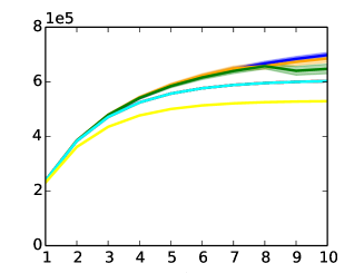
(a) Uniform

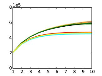
(b) Two steps: $\frac{1}{2k}\times\frac{k}{2}\cup\frac{3}{2k}\times\frac{k}{2}$

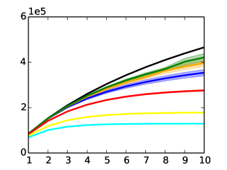
(c) Zipf-$1$: $p_{i}\propto\frac{1}{i}$

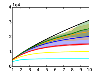
(d) Zipf-$1.5$: $p_{i}\propto\frac{1}{i^{1.5}}$

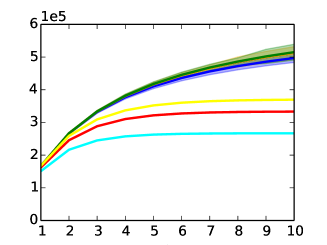
(e) Dirichlet-$1$ prior

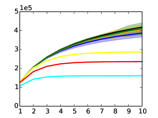
(f) Dirichlet-$1/2$ prior

True value	Previous		Proposed
	Chao-Lee		Poisson smoothing
	ACE		Binomial smoothing $q=1/(t+1)$
	Jackknife		Binomial smoothing $q=2/(t+2)$

Figure 5: Comparisons of the estimated number of unseen species as a function of $t$. All experiments have distribution support size $10^{6}$, $n=5\cdot 10^{5}$, and are averaged over $100$ iterations.

Of the proposed estimators, the binomial-smoothing estimator with parameter $q=\frac{2}{2+t}$ has a stronger theoretical guarantee and performs slightly better than the others. Hence when considering real data we plot only its performance and compare it with the other state-of-the art estimators. We test the estimators on three real datasets taken from various scientific applications where the samples size $n$ ranges from few hundreds to a million. For all these date sets, our estimator outperforms the existing procedures.

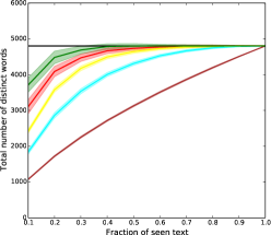
(a) Hamlet random

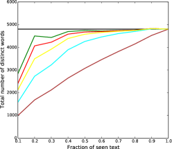
(b) Hamlet consecutive

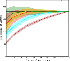
(c) SLOTUs

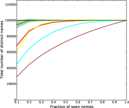
(d) Last names

True value	Previous		Proposed
	Chao-Lee		Binomial smoothing $q=2/(t+2)$
	ACE
	Jackknife
	Empirical

Figure 6: Estimates for number of: $(a)$ distinct words in Hamlet with random sampling $(b)$ distinct words in Hamlet with consecutive sampling $(c)$ SLOTUs on human skin $(d)$ last names.

Figure 6(a) shows the first real-data experiment, predicting vocabulary size based on partial text. Shakespeare’s play Hamlet consists of $n_{\text{total}}=31999$ words, of which $4804$ are distinct. We randomly select $n$ of the $n_{\text{total}}$ words without replacement, predict the number of unseen words in $n_{\text{total}}-n$ new ones, and add it to those observed. The results shown are averaged over $100$ trials. Observe that the new estimator outperforms existing ones and that as little as $20\%$ of the data already yields an accurate estimate of the total number of distinct words. Figure 6(b) repeats the experiment but instead of random sampling, uses the first $n$ consecutive words, with similar conclusions.

Figure 6(c) estimates the number of bacterial species on the human skin. [GTPB07] considered forearm skin biota of six subjects. They identified $n_{\text{total}}=1221$ clones consisting of $182$ different species-level operational taxonomic units (SLOTUs). As before, we select $n$ out of the $n_{\text{total}}$ clones without replacement and predict the number of distinct SLOTUs found. Again the estimates are more accurate than those of existing estimators and are reasonably accurate already with $20\%$ of the data.

Finally, Figure 6(d) considers the 2000 United States Census [Bur14], which lists all U.S. last names corresponding to at least 100 individuals. With these many repetitions, even just a small fraction of the data will cover all names, hence we first subsampled the data $n_{\text{total}}=10^{6}$ and obtained a list of 100328 distinct last names. As before we estimate for this number using $n$ randomly chosen names, again with similar conclusions.

Appendix A Proof of Lemma 4

Proof.

To rigorously prove an impossibility result for the truncated GT estimator, we demonstrate a particular distribution under which the bias is large. Consider the uniform distribution over $n/({\ell}+1)$ symbols, where $\ell$ is a non-zero even integer. By Lemma 3, for this distribution the bias is

$$\mathbb{E}[U-U^{\ell}] =\sum_{x}e^{-\lambda_{x}}(1-e^{-\lambda_{x}t}-h(\lambda_{x}))$$

$$=\frac{n}{{\ell}+1}e^{-({\ell}+1)}\left(1-e^{-({\ell}+1)t}+\sum^{\ell}_{i=1}\frac{(-({\ell}+1)t)^{i}}{i!}\right)$$

$$\geq\frac{n}{{\ell}+1}e^{-({\ell}+1)}\left(\sum^{\ell}_{i=1}\frac{(-({\ell}+1)t)^{i}}{i!}\right)$$

$$\stackrel{{\scriptstyle(a)}}{{\geq}}\frac{n}{{\ell}+1}e^{-({\ell}+1)}\left(\frac{(({\ell}+1)t)^{\ell}}{\ell!}-\frac{(({\ell}+1)t)^{\ell-1}}{(\ell-1)!}\right)$$

$$\geq\frac{n}{({\ell}+1)}e^{-({\ell+1})}\frac{(({\ell}+1)t)^{\ell}}{\ell!}\cdot\frac{(t-1)}{t}$$

$$\geq\frac{n}{3(\ell+1)^{3/2}}t^{\ell}\frac{(t-1)}{t}\geq\frac{n}{3\cdot 2^{3/2}}\frac{t^{\ell}}{\ell^{3/2}}\frac{(t-1)}{t},$$

where $(a)$ follows from the fact that $\frac{(-({\ell}+1)t)^{i}}{i!}$ for $i=1,\ldots,\ell$ is an alternating series with increasing magnitude of terms. Hence

$$\mathbb{E}[U-U^{\ell}]\geq\frac{n}{3\cdot 2^{3/2}}\frac{(t-1)}{t}\min_{\ell\in\{2,4,\ldots\}}\frac{t^{\ell}}{\ell^{3/2}}.$$

For $t\geq 2$, the above minimum occurs at $\ell=2$ and hence $\min_{\ell\in\{2,4,\ldots\}}\frac{t^{\ell}}{\ell^{3/2}}\geq\frac{(t-1)^{3/2}}{2^{3/2}}$. For $1<t<2$, using the fact that $e^{y}\geq ey$ for $y>0$ and $\log t\geq(t-1)\log 2$ for $1<t<2$, we have $\min_{\ell\in\{2,4,\ldots\}}\frac{t^{\ell}}{\ell^{3/2}}\geq(\frac{2e\log t}{3})^{3/2}\geq(\frac{2e\log 2(t-1)}{3})^{3/2}$. Thus for any even value of $\ell>0$,

$$\mathbb{E}[U-U^{\ell}]\geq\frac{n(t-1)^{5/2}}{6.05t}.$$

A similar argument holds for odd values of $\ell$ and $\ell=0$, showing that $|\mathbb{E}[U-U^{\ell}]|\gtrsim\frac{n(t-1)^{5/2}}{t}$ and hence the desired NMSE bound. ∎

References

- [AS64] M. Abramowitz and I. A. Stegun. Handbook of mathematical functions with formulas, graphs, and mathematical tables. Wiley-Interscience, New York, NY, 1964.
- [BF93] John Bunge and M Fitzpatrick. Estimating the number of species: a review. Journal of the American Statistical Association, 88(421):364–373, 1993.
- [BH84] A. D. Barbour and Peter Hall. On the rate of poisson convergence. Mathematical Proceedings of the Cambridge Philosophical Society, 95:473–480, 5 1984.
- [Bur14] United States Census Bureau. Frequently occurring surnames from the Census 2000, 2014.
- [CCG+12] Robert K Colwell, Anne Chao, Nicholas J Gotelli, Shang-Yi Lin, Chang Xuan Mao, Robin L Chazdon, and John T Longino. Models and estimators linking individual-based and sample-based rarefaction, extrapolation and comparison of assemblages. Journal of Plant Ecology, 5(1):3–21, 2012.
- [Cha84] Anne Chao. Nonparametric estimation of the number of classes in a population. Scandinavian Journal of statistics, pages 265–270, 1984.
- [Cha05] Anne Chao. Species estimation and applications. Encyclopedia of statistical sciences, 2005.
- [CL92] Anne Chao and Shen-Ming Lee. Estimating the number of classes via sample coverage. Journal of the American statistical Association, 87(417):210–217, 1992.
- [CL11] T.T. Cai and M. G. Low. Testing composite hypotheses, Hermite polynomials and optimal estimation of a nonsmooth functional. The Annals of Statistics, 39(2):1012–1041, 2011.
- [DF80] P. Diaconis and D. Freedman. Finite exchangeable sequences. Ann. Probab., 8(4):745–764, 08 1980.
- [ET76] B. Efron and R. Thisted. Estimating the number of unseen species: How many words did shakespeare know? Biometrika, 63(3):435–447, 1976.
- [FCW43] Ronald Aylmer Fisher, A Steven Corbet, and Carrington B Williams. The relation between the number of species and the number of individuals in a random sample of an animal population. The Journal of Animal Ecology, pages 42–58, 1943.
- [FH07] Dinei Florencio and Cormac Herley. A large-scale study of web password habits. In Proceedings of the 16th international conference on World Wide Web, pages 657–666. ACM, 2007.
- [Goo53] Irving John Good. The population frequencies of species and the estimation of population parameters. Biometrika, 40(3-4):237–264, 1953.
- [GT56] I.J. Good and G.H. Toulmin. The number of new species, and the increase in population coverage, when a sample is increased. Biometrika, 43(1-2):45–63, 1956.
- [GTPB07] Zhan Gao, Chi-hong Tseng, Zhiheng Pei, and Martin J Blaser. Molecular analysis of human forearm superficial skin bacterial biota. Proceedings of the National Academy of Sciences, 104(8):2927–2932, 2007.
- [HHRB01] Jennifer B Hughes, Jessica J Hellmann, Taylor H Ricketts, and Brendan JM Bohannan. Counting the uncountable: statistical approaches to estimating microbial diversity. Applied and environmental microbiology, 67(10):4399–4406, 2001.
- [HNSS95] Peter J Haas, Jeffrey F Naughton, S Seshadri, and Lynne Stokes. Sampling-based estimation of the number of distinct values of an attribute. In VLDB, volume 95, pages 311–322, 1995.
- [ILLL09] Iuliana Ionita-Laza, Christoph Lange, and Nan M Laird. Estimating the number of unseen variants in the human genome. Proceedings of the National Academy of Sciences, 106(13):5008–5013, 2009.
- [JVHW15] Jiantao Jiao, Kartik Venkat, Yanjun Han, and Tsachy Weissman. Minimax estimation of functionals of discrete distributions. IEEE Transactions on Information Theory, 61(5):2835–2885, 2015.
- [KLR99] Ian Kroes, Paul W Lepp, and David A Relman. Bacterial diversity within the human subgingival crevice. Proceedings of the National Academy of Sciences, 96(25):14547–14552, 1999.
- [Kol86] Gina Kolata. Shakespeare’s new poem: An ode to statistics. Science (New York, NY), 231(4736):335, 1986.
- [LNS99] Oleg Lepski, Arkady Nemirovski, and Vladimir Spokoiny. On estimation of the norm of a regression function. Probability Theory and Related Fields, 113(2):221–253, 1999.
- [MS00] David A. McAllester and Robert E. Schapire. On the convergence rate of good-turing estimators. In In the Proc. of the Conference on Learning Theory, pages 1–6, 2000.
- [OS15] Alon Orlitsky and Ananda Theertha Suresh. Competitive distribution estimation: Why is Good-Turing good. In Advances in Neural Information Processing Systems, pages 2134–2142, 2015.
- [PBG+01] Bruce J Paster, Susan K Boches, Jamie L Galvin, Rebecca E Ericson, Carol N Lau, Valerie A Levanos, Ashish Sahasrabudhe, and Floyd E Dewhirst. Bacterial diversity in human subgingival plaque. Journal of bacteriology, 183(12):3770–3783, 2001.
- [RCS+09] Harlan S Robins, Paulo V Campregher, Santosh K Srivastava, Abigail Wacher, Cameron J Turtle, Orsalem Kahsai, Stanley R Riddell, Edus H Warren, and Christopher S Carlson. Comprehensive assessment of T-cell receptor -chain diversity in t cells. Blood, 114(19):4099–4107, 2009.
- [Rob68] Herbert E Robbins. Estimating the total probability of the unobserved outcomes of an experiment. The Annals of Mathematical Statistics, 39(1):256–257, 1968.
- [RRSS09] Sofya Raskhodnikova, Dana Ron, Amir Shpilka, and Adam Smith. Strong lower bounds for approximating distribution support size and the distinct elements problem. SIAM Journal on Computing, 39(3):813–842, 2009.
- [SCL03] Tsung-Jen Shen, Anne Chao, and Chih-Feng Lin. Predicting the number of new species in further taxonomic sampling. Ecology, 84(3):798–804, 2003.
- [sta92] Stanford statistics department brochure, 1992. https://statistics.stanford.edu/sites/default/files/1992_StanfordStatisticsBrochure.pdf.
- [Ste86] J. Michael Steele. An Efron-Stein inequality for nonsymmetric statistics. Ann. Statist., 14(2):753–758, 06 1986.
- [SvB84] Eric P Smith and Gerald van Belle. Nonparametric estimation of species richness. Biometrics, pages 119–129, 1984.
- [TE87] Ronald Thisted and Bradley Efron. Did shakespeare write a newly-discovered poem? Biometrika, 74(3):445–455, 1987.
- [VV11] Gregory Valiant and Paul Valiant. Estimating the unseen: an -sample estimator for entropy and support size, shown optimal via new CLTs. In Proceedings of the 43rd annual ACM symposium on Theory of computing, pages 685–694, 2011.
- [VV13] Paul Valiant and Gregory Valiant. Estimating the unseen: Improved estimators for entropy and other properties. In Advances in Neural Information Processing Systems, pages 2157–2165, 2013.
- [VV15] Gregory Valiant and Paul Valiant. Instance optimal learning. arXiv preprint arXiv:1504.05321, 2015.
- [WY15a] Yihong Wu and Pengkun Yang. Chebyshev polynomials, moment matching, and optimal estimation of the unseen. preprint arxiv:1504.01227, Apr. 2015.
- [WY15b] Yihong Wu and Pengkun Yang. Minimax rates of entropy estimation on large alphabets via best polynomial approximation. to appear in IEEE Transactions on Information Theory, arxiv:1407.0381, Jul 2015.