Quantum Corrections to Holographic Mutual Information

Abstract:

We compute the leading contribution to the mutual information (MI) of two disjoint spheres in the large distance regime for arbitrary conformal field theories (CFT) in any dimension. This is achieved by refining the operator product expansion method introduced by Cardy [1]. For CFTs with holographic duals the leading contribution to the MI at long distances comes from bulk quantum corrections to the Ryu-Takayanagi area formula. According to the FLM proposal[2] this equals the bulk MI between the two disjoint regions spanned by the boundary spheres and their corresponding minimal area surfaces. We compute this quantum correction and provide in this way a non-trivial check of the FLM proposal.

1 Introduction

It is well known that the mutual information for disjoint and compact regions in holographic theories undergoes a sharp transition when the separation distance is larger than some characteristic scale $r_{c}$ [3]. The usual Ryu-Takayanagi formula for the entanglement entropy gives a zero contribution to the mutual information for $r>r_{c}$ and therefore we expect the leading non-zero answer to be determined by quantum fluctuations in the dual space-time. As proposed by Faulkner, Lewkowycz and Maldacena (FLM) [2] such contributions at leading order are given by the mutual information between the bulk regions depicted in Figure 1.

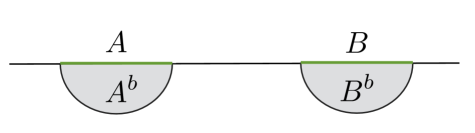
Figure 1: This paper studies the MI between the boundary regions $A,B$. The FLM proposal predicts the non-zero contribution to the MI for $r>r_{c}$ is given by the bulk MI between the hemispherical regions $A_{b}$ and $B_{b}$ contained within the Ryu-Takayanagi minimal surfaces.

While FLM gives us an in principle prescription for calculating quantum corrections to entanglement entropy actually carrying out such computations is technically challenging. In three bulk dimensions alternative methods to compute quantum corrections to MI are available [9]. This approach is based on computing the one-loop determinant of the bulk partition function in the geometries constructed in [10], and has been extensively and successfully applied in a large variety of situations [11, 12, 13, 14, 15, 16, 17, 18, 19] finding agreement with independent CFT calculations. It should be emphasized that the approach of [9] is quite different to FLM. It is expected that the two approaches should agree for 2d CFTs, however this has never been explicitly demonstrated. Additionally, the one loop determinant methods are essentially out of reach in higher dimensions. It is thus of fundamental importance to develop techniques that allow us to carry out computations with the FLM proposal, and to check the results against boundary CFT calculations where available.

An obvious difficulty this program faces is the lack of CFT results for entanglement entropy/mutual information in CFT’s that one could use to compare with their corresponding holographic predictions. We plan to remedy this situation and the first result we would like to present is the leading correction to MI in the limit of large distances $r$ between the two spherical shaped regions in any CFT:

$$I=\mathcal{N}_{\Delta}\frac{\sqrt{\pi}\Gamma(2\Delta+1)}{4\Gamma(2\Delta+\frac{3}{2})}\frac{(R_{A}R_{B})^{2\Delta}}{r^{4\Delta}}+\ldots$$ (1)

where $\Delta$ is the scaling dimension of the lowest dimension scalar operator, $R_{A}$ and $R_{B}$ are the radius of the two spheres and $\mathcal{N}_{\Delta}$ is the number/degeneracy of such real scalar operators. We use the framework setup by Cardy for calculating MI in higher dimensions [1]. While the scale dependent part of (1) was established in [1] and in the earlier numerical work of [20], the exact pre-factor was left unknown, except for some results in free theories. Surprisingly the pre-factor we find is the same as in $2d$ CFTs [21].

The methods of [1] have been applied in a variety of situations to compute Rényi mutual information and mutual information for free scalars and fermions at zero and finite temperature [22, 23, 24, 25, 26]. The main tool is an operator product expansion argument used to express the Rényi mutual information in terms of multi-correlators of the different fields in the replicated geometry [3, 21, 1]. The new ingredient we add to this discussion is a method to find the analytic continuation in the replica parameter $n$ of sums of the OPE coefficients that works for any CFT. This continuation is inspired by recent results for computing perturbative corrections to EE [27, 28].

Turning to the bulk FLM computation we find that the framework of [1] can also be used to compute the leading term of the bulk mutual information for disjoint hemispheres in arbitrary space-time dimensions. We consider only the contribution coming from a free scalar field living on the $AdS_{d+1}$ background, where the mass of the scalar is related to the conformal dimension of the dual operator in the usual way. Interestingly, the curved geometry does not represent any obstacle in carrying out this calculation and therefore opens the door to a larger exploration of mutual information in curved geometries. These two independent results agree perfectly and therefore provide important evidence for the validity of FLM.

The organization of this paper goes as follows: in section 2, we present a brief overview of the general framework for computing mutual information of disjoint regions in a large distance expansion, following closely the presentation of [1]. In section 3 we present a detailed calculation of the coefficient of the leading term in the mutual information for disjoint spheres in arbitrary CFT and for any dimension. The equivalent dual bulk computation, that is the mutual information between hemispheres in the AdS background, is presented in the section 4.

2 Mutual Information expansion

In this section we briefly review the general framework to compute the mutual information between disjoint regions in quantum field theories following closely [1]. We take the QFT to live on a (potentially) curved $d$ dimensional manifold $\mathcal{M}$.

The Rényi entropy for a given region $X$ is given by

$$S^{(n)}_{X}=\frac{1}{1-n}\log{\rm Tr}_{{\cal H}_{X}}\rho^{n}_{X}$$ (2)

where ${\cal H}_{X}$ is the Hilbert space associated to the region $X$ and $\rho_{X}$ is the reduced density matrix describing the degrees of freedom living in $X$. When $n$ is an integer this quantity can be expressed in terms of a path-integral on a conifold defined by taking $n$ copies of the QFT on $\mathcal{M}^{\otimes n}$ and sewing them together along the region $X$. The Rényi entropies are given by

$$S^{(n)}_{X}=\frac{1}{1-n}\log\left(\frac{Z({\cal C}^{(n)}_{X})}{Z^{n}}\right)\,,$$ (3)

where $Z$ is the partition function on the original space, and $Z({\cal C}^{(n)}_{X})$ is the partition function on the conifold. We are interested in the mutual information $I(A,B)$ associated to two disjoint regions $A$ and $B$, which can be defined as

$$I(A,B)\equiv\lim_{n\to 1}I^{(n)}(A,B)$$ (4)

where $I^{(n)}(A,B)$ is the Rényi mutual information given by:

$$I^{(n)}(A,B)\equiv S_{A}^{(n)}+S_{B}^{(n)}-S_{A\cup B}^{(n)}$$ (5)

or in terms of path integrals

$$I^{(n)}(A,B)=\frac{1}{1-n}\log\left(\frac{Z({\cal C}^{(n)}_{A\cup B})Z^{n}}{Z({\cal C}^{(n)}_{A})Z({\cal C}^{(n)}_{B})}\right)\,.$$ (6)

Part of the difficulty of this calculation is coming up with an analytic continuation in $n$ away from the integers in order to properly take the limit (4). We will address this issue shortly. Further simplification occurs in the limit where the distance between objects $r$ is much larger than the individual sizes $R_{A},R_{B}$. In that situation we can think of the sewing operation in the region $B$ as seen from the point of view of $A$ as a semi-local operation that couples the n QFTs. That is

$$\frac{Z({\cal C}^{(n)}_{A\cup B})}{Z^{n}}=\langle\Sigma_{A}^{(n)}\Sigma_{B}^{(n)}\rangle_{\mathcal{M}^{n}}$$ (7)

where we make the replacement:

$$\Sigma_{A}^{(n)}=\frac{Z({\cal C}_{A}^{(n)})}{Z^{n}}\sum_{\{k_{j}\}}C_{\{k_{j}\}}^{A}\prod_{j=0}^{n-1}\Phi^{(j)}_{k_{j}}(r_{A})$$ (8)

and $\Phi^{(j)}_{k_{j}}(r_{A})$ is a complete set of operators in the $j$th copy of the QFT located at a conveniently chosen point $r_{A}$ in region $A$. By making appropriate subtractions we can take these operators to have vanishing one point functions on $\mathcal{M}$. An arbitrary product of operators far from $A$ in the conifold geometry of region $A$ is therefore given by

$$\langle\prod_{j^{\prime}=0}^{n-1}\Phi^{(j^{\prime})}_{k^{\prime}_{j^{\prime}}}(r)\rangle_{{\cal C}^{(n)}_{A}} = \langle\prod_{j^{\prime}=0}^{n-1}\Phi^{(j^{\prime})}_{k^{\prime}_{j^{\prime}}}(r)\sum_{\{k_{j}\}}C_{\{k_{j}\}}^{A}\prod_{j=0}^{n-1}\Phi^{(j)}_{k_{j}}(r_{A})\rangle_{\mathcal{M}^{\otimes n}}$$ (9)

$$= \sum_{\{k_{j}\}}C_{\{k_{j}\}}^{A}\prod_{j}\langle\Phi_{k^{\prime}_{j}}(r)\Phi_{k_{j}}(r_{A})\rangle_{\cal M}$$

As pointed out by Cardy this equation is true for any arbitrary QFT, however for a CFT in flat space we can use scalar operators with the following normalization

$$\langle\Phi_{k^{\prime}}(r)\Phi_{k}(r_{A})\rangle_{\mathbb{R}^{d}}=\frac{\delta_{kk^{\prime}}}{|r-r_{A}|^{2x_{k}}}\,.$$ (10)

Plugging (10) into (9) allows us to extract the coefficients of interest

$$C_{\{k_{j}\}}^{A}=\lim_{r\to\infty}|r|^{2\sum_{j}x_{k_{j}}}\langle\prod_{j^{\prime}}\Phi^{(j)}_{k_{j}}(r)\rangle_{{\cal C}^{(n)}_{A}}\,$$ (11)

and with them we can write a formal expression for the ratio of partition functions required for the evaluation of the Rényi mutual information

$$\frac{Z({\cal C}^{(n)}_{A\cup B})Z^{n}}{Z({\cal C}^{(n)}_{A})Z({\cal C}^{(n)}_{B})}=\sum_{\{k_{j}\}}{C^{A}_{\{k_{j}\}}}{C^{B}_{\{k_{j}\}}}r^{-2\sum_{j}x_{k_{j}}}\,.$$ (12)

Assuming a $\mathbf{Z}_{2}$ symmetry for the lowest dimension operator in the CFT, say $\mathcal{O}$, ( $\mathbf{Z}_{2}$ acts as $\mathcal{O}(r)\to-\mathcal{O}(r)$) such that the symmetry is not spontaneously broken in the replica manifold, then $\langle\mathcal{O}^{(j)}(r)\rangle_{{\cal C}^{A}_{n}}=0$. Thus the first contribution to (12) comes from replacing each of the $\Sigma^{(n)}_{A,B}$ with two operator insertions of $\mathcal{O}$ on the different replicas $j,j^{\prime}=0,\ldots n-1$ and is therefore given by

$$\frac{Z({\cal C}^{(n)}_{A\cup B})Z^{n}}{Z({\cal C}^{(n)}_{A})Z({\cal C}^{(n)}_{B})}=1+\frac{1}{2}\sum_{j\neq j^{\prime}}{C^{A}_{jj^{\prime}}}{C^{B}_{jj^{\prime}}}r^{-4\Delta}+\ldots\,,$$ (13)

where the factor of $1/2$ appears to account for the double counting in the sum, and the number 1 comes from the contribution to (11) where all $\Phi_{k}(r)=\mathbf{1}$.

Using (11) the coefficients $C_{jj^{\prime}}$ are simply

$$C_{jj^{\prime}}^{A}=\lim_{r\to\infty}|r|^{4\Delta}\langle\mathcal{O}^{(j)}(r)\mathcal{O}^{(j^{\prime})}(r)\rangle_{{\cal C}^{(n)}_{A}}\,.$$ (14)

where $\Delta$ is the lowest scaling dimension of the CFT operators and then (13) just depends on two point functions in the conifold manifold. The first non-trivial contribution to the mutual information is

$$I(A,B) = \lim_{n\to 1}\frac{1}{1-n}\left(\frac{n}{2}\sum_{j=1}^{n-1}{C^{A}_{0j}}{C^{B}_{0j}}\right)r^{-4\Delta}+\ldots$$ (15)

where we have used the cyclicity of the replica manifold to reduced the double sum to a single one.

3 CFT in Euclidean space

In this section we evaluate the leading term in the mutual information (15), when $A\cup B$ is a system of two largely separated $d-1$ spheres. In our setup we will consider an arbitrary CFT in flat euclidean geometry with $d$ dimensions. Our starting point uses the conformal transformation introduced in [29], to map two point correlation functions in the conifold associated to a single entangling sphere to finite temperature two point functions in Hyperbolic space. As shown in [27], sums over the replica manifold of thermal Green functions can be computed by using their analyticity properties as well as its exact form for ($n=1$), which is the one that can be conformally mapped to a two point function in flat euclidean space. We use a method similar to that of [27], to evaluate the limiting sum in (15).

Thinking in terms of embedding coordinates (we use the notation and conventions given in [27]) the map between $\mathbb{R}^{d}$ and $\mathbb{S}^{1}\times\mathbb{H}^{d-1}$ can be stated as follow

$$P|_{H}=\Omega P|_{E}$$ (16)

where $P$ is a point lying in the upper projective light cone of $\mathbb{R}^{1,d+1}$ with $P|_{E}$, $P|_{H}$ corresponding to its representation in terms of Euclidean and Hyperbolic coordinates respectively, and $\Omega=R^{-1}(Y^{I}+\cos\tau)$ is the conformal factor that relates them both. More specifically

$$P|_{E}=\left(\frac{R^{2}+x^{2}}{2R},\frac{R^{2}-x^{2}}{2R},x^{\mu}\right),\qquad x^{\mu}\in\mathbb{R}^{d}$$ (17)

and

$$P|_{H}=\left(Y^{I},\cos\tau,\sin\tau,Y^{m}\right),\qquad(Y^{I},Y^{m})\in\mathbb{H}^{d-1}$$ (18)

where $\mathbb{H}^{d-1}$ is defined as the locus $-(Y^{I})^{2}+Y^{m}Y^{m}=-1$ and $Y^{I}>0$ with $m=1,\cdots d-1$, and $\tau$ is the coordinate on the $\mathbb{S}^{1}$ where $\tau\equiv\tau+2\pi$. While this conformal mapping is appropriate for a CFT living on flat space, it can be extended to the conifold geometry ${\cal C}^{(n)}_{A}$ simply by making the $\tau$ circle larger such that $\tau\equiv\tau+2\pi n$.

At the level of the two point functions in the conifold geometry the statement is

$$\langle{\cal O}(x_{a}){\cal O}(x_{b})\rangle_{{\cal C}^{(n)}_{A}}=\Omega^{\Delta}(a)\Omega^{\Delta}(b)G_{n}(\tau_{b}-\tau_{a};Y_{a}\cdot Y_{b})$$ (19)

where $G_{n}$ is the thermal Green function in hyperbolic space associated to the operator $\cal O$ at temperature $T=1/2\pi n$. That is

$$G_{n}(\tau_{b}-\tau_{a};Y_{a}\cdot Y_{b})={\rm tr}\left(e^{-2\pi nH}{\cal T}{\cal O}(i\tau_{a},Y_{a}){\cal O}(i\tau_{b},Y_{b})\right)$$ (20)

where $\cal T$ is for the euclidean time ordering operation. We want to use this relation to evaluate the leading contribution to (15). Note that while the conformal factors are only well defined if $n$ is an integer, the thermal green’s function is defined for any $n$ and this will be the key feature that allows us to analytically continue the sums in (15). Further, while $G_{n}$ is an unknown theory dependent function, all we will need in order to compute the MI is the thermal greens function at $n=1$ which is known.

The explicit expression for the thermal Green function at $T=1/2\pi$ is,

$$G_{1}(\tau;Y_{a}\cdot Y_{b})=\frac{c_{\Delta}}{(-2Y_{a}\cdot Y_{b}-2\cos(\tau))^{\Delta}}\,,$$ (21)

where it is easy to show that $c_{\Delta}=1$ due to the normalization given in (10). The point $r$ far away from region $A$ on the $j$’th replica maps under (16) to:

$$\left(\tau=\pi(2j-1),Y_{I}\rightarrow 1\right)\quad{\rm with}\quad|r|\sim 2^{1/2}R(Y_{I}-1)^{-1/2}$$ (22)

This allows us to write the OPE coefficients (14) in terms of the thermal Green functions

$$C_{jj^{\prime}} = \lim_{Y^{I}\to 1}(R)^{4\Delta}2^{2\Delta}(Y_{I}-1)^{-2\Delta}\Omega^{2\Delta}(\pi,Y_{I})G_{n}(2\pi(j-j^{\prime});-1)$$ (23)

$$= (2R)^{2\Delta}G_{n}(2\pi(j-j^{\prime}))$$

where we used the simplified notation $G_{n}(\tau)\equiv G_{n}(\tau;Y_{a}\cdot Y_{b}=-1)$. The mutual information in terms of the thermal Green functions is therefore given by:

$$I(A,B)=\lim_{n\to 1}\frac{(4R_{A}R_{B})^{2\Delta}}{2|r_{A}-r_{B}|^{4\Delta}}\frac{1}{1-n}\left(\sum_{j=1}^{n-1}G^{2}_{n}(2\pi j)\right)+\ldots\,.$$ (24)

This quantity can be evaluated following similar steps to the calculation of [27] with some obvious modifications.

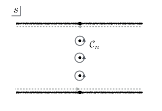
Figure 2: Integration contour used to evaluate the sum in 24.

To start with we use the unique analytic continuation of the thermal green function to the complex time plane $G_{n}(\tau)\to G_{n}(-is)$ with $s\in\mathbb{C}$ and $0<\textrm{Im}(s)<2\pi n$ and expressed the sum as a contour integral

$$\sigma_{n}\equiv\sum_{j=1}^{n-1}G^{2}_{n}(2\pi j)=\int_{{\cal C}_{n}}\frac{ds}{2\pi i}\frac{G^{2}_{n}(-is)}{e^{s}-1}$$ (25)

where ${\cal C}_{n}$ is the prescribed contour in figure 2. At this point it is convenient to make a convenient subtraction from the integrand in (25) which leads to a vanishing contribution to the integral due to the absence of poles within the contour ${\cal C}_{n}$:

$$\sigma_{n}=\int_{{\cal C}_{n}}\frac{ds}{2\pi i}G^{2}_{n}(-is)k_{n}(s)\qquad k_{n}(s)\equiv\left(\frac{1}{e^{s}-1}-\frac{1}{e^{s/n}-1}\right)$$ (26)

This subtraction ensures that the kernel $k_{n}(s)$ vanishes when $n=1$. Assuming the integrand goes to zero when $\textrm{Re}(s)\to\pm\infty$ we can deform the integration contour to the lines with ${\Im}s=\epsilon,2\pi n-\epsilon$ just above and below the branch cuts that are expected to appear in the thermal Greens function:

$$\sigma_{n}=\int_{-\infty}^{\infty}\frac{ds}{2\pi i}\left(G^{2}_{n}(-is+\epsilon)k_{n}(s+i\epsilon)-G^{2}_{n}(-is-\epsilon)k_{n}(s-i\epsilon)\right)$$ (27)

where $\epsilon>0$. We have additionally used the $2\pi n$ periodicity of $G^{2}_{n}$ and $k_{n}$ in the complex plane setting $e^{2\pi in}=1$ which is true prior to analytic continuation in $n$.

The limit of interest can now be taken:

$$\lim_{n\to 1}\frac{1}{n-1}\sigma_{n}=\int_{-\infty}^{\infty}\frac{ds}{2\pi i}\left(G^{2}_{1}(-is+\epsilon)\hat{k}(s+i\epsilon)-G^{2}_{1}(-is-\epsilon)\hat{k}(s-i\epsilon)\right)$$ (28)

where:

$$\qquad\hat{k}(s)\equiv-\frac{1}{4\sinh^{2}(s/2)}\,.$$ (29)

The last step is to deform the integration contour in the first term to ${\Im}s=\pi$ and ${\Im}s=-\pi$ in the second term. This is convenient since $G_{1}^{2}(-is^{\prime}+\pi)=G_{1}^{2}(-is^{\prime}-\pi)$ and these are non singular when $s^{\prime}=0$ so we have dropped the $i\epsilon$’s. This leads to the final answer:

$$\lim_{n\to 1}\frac{1}{n-1}\sigma_{n}=\int_{-\infty}^{\infty}ds^{\prime}\frac{G_{1}^{2}(-is^{\prime}+\pi)}{4\cosh^{2}(s^{\prime}/2)}=\int_{-\infty}^{\infty}ds^{\prime}(2\cosh(s^{\prime}/2))^{-4\Delta-2}$$ (30)

This last integral is in fact convergent and well defined for $\textrm{Re}(\Delta)>-1/2$ and evaluates to:

$$\frac{2\sqrt{\pi}}{4^{2\Delta+1}}\frac{\Gamma(2\Delta+1)}{\Gamma(2\Delta+3/2)}.$$ (31)

Plugging this result into (24), gives the leading term in the mutual information

$$I(A,B)=\frac{\sqrt{\pi}\Gamma(2\Delta+1)}{4\Gamma(2\Delta+\frac{3}{2})}\frac{(R_{A}R_{B})^{2\Delta}}{|r_{A}-r_{B}|^{4\Delta}}+\ldots$$ (32)

valid for any CFT. This is a surprising result since it is independent of the space-time dimension of the theory and therefore equals the one for 2D CFTs.

4 Field Theory in the Bulk

In the previous section we found that the leading term in the mutual information between separated spheres in any dimensions depends only on the lowest scaling dimension of the CFT operators. This powerful result gives us a good amount of data to check the FLM prescription as a reliable method to compute quantum corrections to holographic entanglement entropy. This section will focus on carrying out the computation dual to the CFT calculation of the section 3. That is, we perform the calculation of the leading term in the mutual information between separated hemispheres for a scalar QFT in an AdS background geometry.

This calculation fits into the framework described in section 2 as applied to an arbitrary QFT in curved geometry. As described there, an important simplification occurs when the theory is a CFT. However, we argue that such a simplification is irrelevant if we are just interested in the leading term of the mutual information at large separation. The relevant coefficient is still given in terms of the two point correlation functions of operators in the conifold AdS background. This quantity can be computed via an application of the method of images, as described in [1], since in this approximation the bulk quantum fields can be considered to be free.

In section 2 the method to extract the appropriate OPE coefficients involved examining multi-point function of a set of fields in the replicated space at points far from region $A$. Taking the general result (9) and applying it to two identical non-unit operators $\phi$ on distinct replicas $j$ and $j^{\prime}$ this formal expression can be written as

$$\langle\phi^{(j)}(r)\phi^{(j^{\prime})}(r)\rangle_{{\cal C}^{(n)}_{A}} = C_{jj^{\prime}}^{A}\langle\phi(r)\phi(r_{A})\rangle_{{\cal M}}^{2}$$ (33)

$$+\left.\sum_{k_{j},k_{j^{\prime}}}\right.^{\prime}C_{k_{j},k_{j^{\prime}}}^{A}\langle\phi(r)\Phi_{k_{j}}(r_{A})\rangle_{\cal M}\langle\phi(r)\Phi_{k_{j^{\prime}}}(r_{A})\rangle_{\mathcal{M}}\,.$$

where this last sum is over operators distinct from $\phi$, that is $\Phi_{k_{j}},\Phi_{k_{j^{\prime}}}\neq\phi$. Notice that for a CFT the choice of normalization (10) made the later sum in (33) equal to zero unlike in an arbitrary QFT. However, for a free scalar theory, the largest two point function at long distances corresponds to that of the fundamental field $\phi(r)$ with itself, and therefore the two point function between $\phi(r)$ and any other operator of the theory is smaller for large separations. That is, if $r\gg r_{A}$, then

$$\langle{\Phi}_{k_{j},k_{j}^{\prime}}(r)\phi(r_{A})\rangle\ll\langle\phi(r)\phi(r_{A})\rangle\,.$$ (34)

That means that the main contribution to the LHS of (33) is given by the first term in the RHS of (33).

Therefore, by taking $r\to\infty$ we can extract the coefficients $C^{A}_{jj^{\prime}}$:

$$C^{A}_{jj^{\prime}}=\lim_{r\to\infty}G_{1}(r,r_{A})^{-1}G_{1}(r,r_{A})^{-1}\langle\phi^{(j)}(r)\phi^{(j^{\prime})}(r)\rangle_{{\cal C}^{(n)}_{A}}\,.$$ (35)

This quantity determines the first correction to the ratio

$$\frac{Z({\cal C}^{(n)}_{A\cup B})Z^{n}}{Z({\cal C}^{(n)}_{A})Z({\cal C}^{(n)}_{B})}=1+\frac{1}{2}\sum_{jj^{\prime}}{C}^{A}_{jj^{\prime}}{C}^{B}_{jj^{\prime}}G_{1}(r_{A},r_{B})^{2}+\cdots$$ (36)

required for the evaluation of the mutual information up to that order. This is the equivalent of (13) in AdS space-time.

The two point function for a free scalar in the AdS bulk is given by [30]

$$G_{1}(r,r^{\prime})=\frac{2C_{\Delta}}{\nu}\left(\frac{\xi}{2}\right)^{\Delta}F(\frac{\Delta}{2},\frac{\Delta}{2}+\frac{1}{2};\nu;\xi^{2})$$ (37)

where

$$\xi=\frac{2zz^{\prime}}{z^{2}+z^{\prime 2}+(t_{E}-t^{\prime}_{E})^{2}+(x-x^{\prime})^{2}}\,,$$ (38)

where the $d$ boundary theory coordinates in euclidean signature are $(t_{E},x^{\alpha})$ and $x^{\alpha}$ are the spatial coordinates with $\alpha=1,\ldots d-1$. The metric of AdS is given by:

$$ds^{2}=\frac{dz^{2}+dt_{E}^{2}+dx^{2}}{z^{2}}$$ (39)

We also have set $\Delta=\frac{d}{2}+\nu$ and $\nu=\sqrt{\frac{d^{2}}{4}+m^{2}}$.

The two points $r_{A}$ and $r_{B}$ are well separated such that the Greens function becomes in this limit

$$G_{1}(r_{A},r_{B})\approx\frac{2C_{\Delta}}{\nu}\frac{z^{\Delta}_{A}z^{\Delta}_{B}}{|x_{A}-x_{B}|^{2\Delta}}\,.$$ (40)

We can rewrite (36) as

$$\frac{Z({\cal C}^{(n)}_{A\cup B})Z^{n}}{Z({\cal C}^{(n)}_{A})Z({\cal C}^{(n)}_{B})}=1+\frac{1}{2}\sum_{jj^{\prime}}{\tilde{C}}^{A}_{jj^{\prime}}{\tilde{C}}^{B}_{jj^{\prime}}\frac{1}{|x_{A}-x_{B}|^{4\Delta}}+\cdots$$ (41)

where ${\tilde{C}}^{A}_{jj^{\prime}}=\frac{2C_{\Delta}z^{2\Delta}_{A}}{\nu}C^{A}_{jj^{\prime}}$ and similarly for $B$. The mutual information in terms of the tilde coefficients is given by

$$I(A,B) \approx \lim_{n\to 1}\frac{1}{1-n}\left(\frac{1}{2}\sum_{jj^{\prime}}{\tilde{C}^{A}_{jj^{\prime}}}{\tilde{C}^{B}_{jj^{\prime}}}\right)\frac{1}{|x_{A}-x_{B}|^{4\Delta}}\,.$$ (42)

We now focus on evaluating the coefficients ${\tilde{C}}^{A}_{jj^{\prime}}$. Further simplification is possible in the case in which the entangling surface is a hemisphere in AdS. Consider the following inversion transformation

$$x^{\prime\alpha} = \frac{x^{\alpha}+n^{\alpha}R_{A}}{(x+R_{A}n)^{2}+t_{E}^{2}+z^{2}}-\frac{n^{\alpha}}{2R_{A}}\,,\qquad t^{\prime}_{E}=\frac{t_{E}}{(x+R_{A})^{2}+t_{E}^{2}+z^{2}}\,,$$

$$z^{\prime} = \frac{z}{(x+R_{A}n)^{2}+t_{E}^{2}+z^{2}}$$ (43)

where $n^{\alpha}=(1,0,\ldots 0)$ is a $d-1$ dimensional vector. This transformation maps the conifold ${\cal C}^{(n)}_{A}$ with singularities located on the hemisphere $x^{2}+z^{2}=R_{A}^{2}$ at $t_{E}=0$ to a conifold ${\cal C^{\prime}}^{(n)}_{A}$ with singularities located on the plane $(t^{\prime}_{E}=0,x^{\prime 1}=0)$. This later coordinate system is more suitable for some analytic manipulations.

We will apply this to the point $r_{A}$ as well as the point at $r=r_{\infty}\rightarrow\infty$ needed to evaluate (35). The reference point $r_{A}=(z_{A},t_{E},x^{\alpha})$ we can take in the middle of the $A$ hemisphere:

$$\left(z=z_{A},\,t_{E}=0,\,x^{\alpha}=0\right)\rightarrow\left(z^{\prime}=\frac{z_{A}}{R_{A}^{2}+z_{A}^{2}},\,t^{\prime}_{E}=0,\,x^{\prime\alpha}=\frac{n^{\alpha}}{2R_{A}}\frac{R_{A}^{2}-z_{A}^{2}}{(R_{A}^{2}+z_{A}^{2})}\right)$$ (44)

and the point at infinity becomes:

$$r_{\infty}\rightarrow r_{\infty}^{\prime}\approx\left(z^{\prime}=\epsilon,\,t^{\prime}_{E}=0,\,x^{\prime\alpha}=-n^{\alpha}/2R_{A}\right)$$ (45)

where we should take the limit $\epsilon\rightarrow 0$ in order to send $r_{\infty}\rightarrow\infty$. For example in this limit $G_{1}(r^{\prime},r^{\prime}_{A})\rightarrow(\epsilon z_{A})^{\Delta}2C_{\Delta}\nu^{-1}$, such that the OPE coefficients in (35) become

$$C^{A}_{jj^{\prime}}=\lim_{\epsilon\to 0}\epsilon^{-2\Delta}z_{A}^{-2\Delta}\left(\frac{\nu}{2C_{\Delta}}\right)^{2}\langle\phi^{({j})}(r^{\prime})\phi^{(j^{\prime})}(r^{\prime})\rangle_{{\cal C^{\prime}}^{(n)}_{A}}\,.$$ (46)

The tilde coefficients are now

$$\tilde{C}^{A}_{jj^{\prime}}=\lim_{\epsilon\to 0}\epsilon^{-2\Delta}\frac{\nu}{2C_{\Delta}}\langle\phi^{(j)}(r^{\prime})\phi^{(j^{\prime})}(r^{\prime})\rangle_{{\cal C^{\prime}}^{(n)}_{A}}\,$$ (47)

Now, we analyticaly continue $n$ to the values $1/m$ where $m$ is an integer. This allows us to calculate the two point function on ${\cal C^{\prime}}^{(1/m)}_{A}$ using the method of images since the resulting space can be regarded as a $\mathbb{Z}_{m}$ quotient of $AdS$:

$$\langle\phi^{(j)}(r^{\prime})\phi^{(j^{\prime})}(r^{\prime})\rangle_{{\cal C^{\prime}}^{(1/m)}_{A}}=\sum_{k=0}^{m-1}\langle\phi(r^{\prime}[\theta_{j}+2\pi k/m])\phi(r^{\prime}[\theta_{j^{\prime}}])\rangle_{AdS_{d+1}}\,,$$ (48)

where we have dropped the $j$ superscript in the fields since now the fields are defined in a single copy of AdS. The point $r^{\prime}[\theta]$ is defined:

$$r^{\prime}[\theta]=\left(z^{\prime}=\epsilon,\,\,t^{\prime}_{E}=-\sin(\theta)/2R_{A},\,\,x^{\prime\alpha}=-n^{\alpha}\cos(\theta)/2R_{A}\right)$$ (49)

which is a rotation of the point $r^{\prime}_{\infty}$ about the conifold plane by angle $\theta$. The angle $\theta_{j}$ will eventually be set equal to $2\pi j$ since they label the replicas when $n$ is taken to be an integer, however for now we keep $\theta_{j}$ general. Using the $z=\epsilon\to 0$ limit of the AdS green functions as well we can write (48) as

$$\langle\phi^{(j)}(r^{\prime})\phi^{(j^{\prime})}(r^{\prime})\rangle_{{\cal C^{\prime}}^{(1/m)}_{A}}=\frac{2C_{\Delta}}{\nu}\epsilon^{2\Delta}(2R_{A})^{2\Delta}\sum_{k=0}^{m-1}\frac{1}{(2-2\cos(\theta_{j^{\prime}}-\theta_{j}+2\pi k/m))^{\Delta}}\,.$$

We can calculate this last sum again using contour integration methods to write this as:

$$g_{m}(\theta)\equiv\sum_{k=0}^{m-1}\frac{1}{(2-2\cos(\theta+2\pi k/m))^{\Delta}}=\int_{-\infty}^{\infty}\frac{ds}{2\pi i}\left(q_{m}(s+i\delta)-q_{m}(s-i\delta)\right)$$ (50)

where

$$q_{m}(s)=\frac{m}{(e^{(s-i\theta)m}-1)}\frac{1}{(2-2\cosh s)^{\Delta}}$$ (51)

and $\delta$ is a positive infinitesimal parameter. This last expression is then the desired $m$ analytic continuation. Note that this function is periodic in $\theta\equiv\theta+2\pi/m$ so to make sense of the continuation in $m$ it is natural to define $\hat{\theta}=m\theta$ which is then defined for $0<\hat{\theta}<2\pi$. In order to gain confidence in this result we study the $n$ continuation more carefully in Appendix A where we check numerically that the resulting function agrees with the original sum when $m$ is an integer and is well behaved in various limits away from integer $m$.

We can now take $m\rightarrow 1/n$ where $n$ is integer. We will not need to know explicitly the function $g_{1/n}(\theta)$ just that it satisfies certain nice properties. Firstly it is periodic $g_{1/n}(\theta+2\pi n)=g_{1/n}(\theta)$. Secondly when $n=1$ we find:

$$g_{1}(\theta)=\frac{1}{(2-2\cos\theta)^{\Delta}}$$ (52)

and finally it is well behaved (decays exponentially) as $s=i\theta\rightarrow\pm\infty$. Indeed these properties are sufficient for us to apply the same analytic continuation techniques for the replica sum as in Section 3. The tilde coefficients become:

$$\tilde{C}_{jj^{\prime}}=(2R_{A})^{2\Delta}g_{1/n}(2\pi(j-j^{\prime}))$$ (53)

such that the leading correction to the mutual information is:

$$I(A,B)=\frac{(2R_{A})^{2\Delta}(2R_{B})^{2\Delta}}{2|x_{A}-x_{B}|^{4\Delta}}\lim_{n\to 1}\frac{n}{1-n}\sum_{j=1}^{n-1}(g_{1/n}(2\pi j))^{2}$$ (54)

Where this sum is almost identical to (24) in section 3. The main difference is that $G_{n}$, the CFT greens function on $\mathbb{S}^{1}\times\mathbb{H}^{d-1}$, has been replaced by $g_{1/n}$. Since $g_{1/n}$ is $2\pi n$ periodic in $\theta$ it can be considered a thermal Green’s function just like $G_{n}$ and thus analytically continued to the complex $\theta$ plane. Repeating the steps of Section 3 and taking the limit $n\to 1$ we arrive at the identical result to the field theory. We emphasize that $G_{n}$ is different from $g_{1/n}$ (the later is known explicitly while the former is highly theory dependent.) The fact that these different thermal green functions $G_{n}$ and $g_{1/n}$ give rise to the same contribution to the mutual information, is related to the expected agreement between the proposal of [9] and the FLM. We have this established this agreement in the situation at hand.

5 Conclusions

In this work we have presented a set of analytic checks that support the validity of the FLM prescription as applied to the calculation of the leading large distant term in the mutual information between bulk hemispherical regions. This was made possible by providing the CFT counterpart of this calculation, namely, the mutual information between spherical regions in a generic CFT on flat space-time. Notably, the CFT result is universal, and depends only on the lowest scaling dimension of the CFT operators of the theory, and therefore agree with the 2d CFT result.

The methods used in the calculation of the bulk mutual information are expected to be applicable to the computation of similar contributions coming from non-scalar bulk operators, like bulk gravitons. Since there are some critical uncertainties when attempting to apply FLM to gravitons this is an important avenue for further exploration.

Appendix A Analytic continuation of the conifold Green’s function

We gave an expression in (50) for the analytic continuation of $g_{m}(\theta)$ away from integer $m$ where it can be calculated with the method of images. Here we would like to un-package this expression and make some consistency checks.

Firstly the branch cut structure obscures a little the precise definition in (50) and so we give here a slightly more refined version by changing integration variables to $\lambda=e^{s}$ such that:

$$g_{m}(\hat{\theta})=\frac{1}{2\pi i}\int_{C_{+}\cup C_{-}}\frac{d\lambda}{\lambda}\frac{m}{\lambda^{m}e^{-i\hat{\theta}}-1}\left[(-\lambda)^{\Delta}(1-\lambda)^{-2\Delta}\right]$$ (55)

where we take $C_{+}=(0,\infty)+i\delta$ and $C_{-}=(\infty,0)-i\delta$ and pick the branch cuts of the power functions in the standard way to lie on the negative real axis. We have set $\hat{\theta}=\theta m$. Note that it is not convenient to write this as a discontinuity along the branch cut for $\lambda>0$ because this discontinuity itself does not integrate to a finite answer (there is a divergence at $\lambda=1$ for nice values of $\Delta$) and this is regulated by the $i\delta$ prescription. Rather to get a handle on this numerically we can simply rotate the integration contour to $\lambda=e^{i\phi}\mu$ where $\phi={\rm min}[\hat{\theta}/(2m),\pi]$ for the $C_{+}$ contour and $\phi=-{\rm min}[(2\pi-\hat{\theta})/(2m),\pi]$ for the $C_{-}$ contour and we should integrate from $\mu=0$ to $\infty$. This choice is to avoid poles in $\lambda$ occurring at the roots: $\lambda^{m}e^{-i\hat{\theta}}-1=0$. We are assuming $0<\hat{\theta}<2\pi$ for this discussion which is sufficient because of the periodicity of $g_{m}(\hat{\theta})$. This is the definition we work with numerically.

We have checked for several values of $\Delta$ that indeed this does agree with the sum in (50) when $m$ is an integer. It is also clear that $g_{m}(\hat{\theta})$ is an analytic function of $m$ for ${\rm Re}(m)>0$ and for large $m$ behaves as $\sim m^{2\Delta}$ which at least gives it some nice properties that one might believe defines it uniquely.

The final thing to check is the behavior for the real time Greens function: $\hat{\theta}\rightarrow i\eta$ and taking $\eta\rightarrow\pm\infty$. It is not hard to see that:

$$\lim_{\eta\rightarrow\pm\infty}g_{m}(i\eta)\propto e^{-|\eta|\Delta/m}$$ (56)

All of these properties makes this a well defined euclidean thermal green function that we could for example compare to $G_{1/m}$ defined in Section 3.

References

- [1] J. Cardy, “Some results on the mutual information of disjoint regions in higher dimensions,” J.Phys. A46 (2013) 285402, arXiv:1304.7985 [hep-th].
- [2] T. Faulkner, A. Lewkowycz, and J. Maldacena, “Quantum corrections to holographic entanglement entropy,” JHEP 1311 (2013) 074, arXiv:1307.2892.
- [3] M. Headrick, “Entanglement Rényi entropies in holographic theories,” Phys.Rev. D82 (2010) 126010, arXiv:1006.0047 [hep-th].
- [4] B. Swingle, L. Huijse, and S. Sachdev, “Entanglement entropy of compressible holographic matter: loop corrections from bulk fermions,” Phys. Rev. B90 (2014) no.~4, 045107, arXiv:1308.3234 [hep-th].
- [5] S. Leichenauer, “Thermal Corrections to Entanglement Entropy from Holography,” arXiv:1502.07348 [hep-th].
- [6] B. Swingle and M. Van Raamsdonk, “Universality of Gravity from Entanglement,” arXiv:1405.2933 [hep-th].
- [7] T. Miyagawa, N. Shiba, and T. Takayanagi, “Double-Trace Deformations and Entanglement Entropy in AdS,” arXiv:1511.07194 [hep-th].
- [8] N. Engelhardt and A. C. Wall, “Quantum Extremal Surfaces: Holographic Entanglement Entropy beyond the Classical Regime,” JHEP 01 (2015) 073, arXiv:1408.3203 [hep-th].
- [9] T. Barrella, X. Dong, S. A. Hartnoll, and V. L. Martin, “Holographic entanglement beyond classical gravity,” JHEP 1309 (2013) 109, arXiv:1306.4682 [hep-th].
- [10] T. Faulkner, “The Entanglement Renyi Entropies of Disjoint Intervals in AdS/CFT,” arXiv:1303.7221 [hep-th].
- [11] B. Chen, J.-q. Wu, and Z.-c. Zheng, “Holographic Rényi Entropy of Single Interval on Torus: with W symmetry,” arXiv:1507.00183 [hep-th].
- [12] B. Chen and J.-q. Wu, “Holographic Calculation for Large Interval Rényi Entropy at High Temperature,” arXiv:1506.03206 [hep-th].
- [13] B. Chen and J.-q. Wu, “Large Interval Limit of Rényi Entropy At High Temperature,” arXiv:1412.0763 [hep-th].
- [14] B. Chen and J.-q. Wu, “Single interval Rényi entropy at low temperature,” JHEP 1408 (2014) 032, arXiv:1405.6254 [hep-th].
- [15] M. Beccaria and G. Macorini, “On the next-to-leading holographic entanglement entropy in ,” JHEP 1404 (2014) 045, arXiv:1402.0659 [hep-th].
- [16] B. Chen, F.-y. Song, and J.-j. Zhang, “Holographic Rényi entropy in AdS3/LCFT2 correspondence,” JHEP 1403 (2014) 137, arXiv:1401.0261 [hep-th].
- [17] B. Chen and J.-J. Zhang, “On short interval expansion of Rényi entropy,” JHEP 1311 (2013) 164, arXiv:1309.5453 [hep-th].
- [18] B. Chen, J. Long, and J.-j. Zhang, “Holographic Rényi entropy for CFT with W symmetry,” JHEP 1404 (2014) 041, arXiv:1312.5510 [hep-th].
- [19] E. Perlmutter, “Comments on Rényi entropy in AdS3/CFT2,” JHEP 1405 (2014) 052, arXiv:1312.5740 [hep-th].
- [20] N. Shiba, “Entanglement Entropy of Two Spheres,” JHEP 07 (2012) 100, arXiv:1201.4865 [hep-th].
- [21] P. Calabrese, J. Cardy, and E. Tonni, “Entanglement entropy of two disjoint intervals in conformal field theory II,” J. Stat. Mech. 1101 (2011) P01021, arXiv:1011.5482 [hep-th].
- [22] H. J. Schnitzer, “Mutual Rényi information for two disjoint compound systems,” arXiv:1406.1161 [hep-th].
- [23] C. P. Herzog, “Universal Thermal Corrections to Entanglement Entropy for Conformal Field Theories on Spheres,” JHEP 1410 (2014) 28, arXiv:1407.1358 [hep-th].
- [24] C. P. Herzog and J. Nian, “Thermal corrections to Rényi entropies for conformal field theories,” JHEP 1506 (2015) 009, arXiv:1411.6505 [hep-th].
- [25] C. A. Agón, I. Cohen-Abbo, and H. J. Schnitzer, “Large distance expansion of Mutual Information for disjoint disks in a free scalar theory,” arXiv:1505.03757 [hep-th].
- [26] C. P. Herzog and M. Spillane, “Thermal Corrections to Rényi entropies for Free Fermions,” arXiv:1506.06757 [hep-th].
- [27] T. Faulkner, “Bulk Emergence and the RG Flow of Entanglement Entropy,” JHEP 05 (2015) 033, arXiv:1412.5648 [hep-th].
- [28] T. Faulkner, R. G. Leigh, and O. Parrikar, “Shape Dependence of Entanglement Entropy in Conformal Field Theories,” arXiv:1511.05179 [hep-th].
- [29] H. Casini, M. Huerta, and R. C. Myers, “Towards a derivation of holographic entanglement entropy,” JHEP 05 (2011) 036, arXiv:1102.0440 [hep-th].
- [30] E. D’Hoker and D. Z. Freedman, “Supersymmetric gauge theories and the AdS / CFT correspondence,” in Strings, Branes and Extra Dimensions: TASI 2001: Proceedings, pp. 3–158. 2002. arXiv:hep-th/0201253 [hep-th].