Hysteresis in Random-field Ising model on a
Bethe lattice with a mixed coordination number

Abstract

We study zero-temperature hysteresis in the random-field Ising model on a Bethe lattice where a fraction $c$ of the sites have coordination number $z=4$ while the remaining fraction $1-c$ have $z=3$. Numerical simulations as well as probabilistic methods are used to show the existence of critical hysteresis for all values of $c>0$. This extends earlier results for $c=0$ and $c=1$ to the entire range $0\leq c\leq 1$, and provides new insight in non-equilibrium critical phenomena.

I Introduction

The path-breaking study of zero-temperature hysteresis in the random-field Ising model  sethna1 ; sethna2 ; dahmen ; perkovic ; sethna3 , has enhanced our understanding of a complex system’s response to a slowly varying applied field. It explains several features observed in experiments; hysteresis, Barkhausen noise, return point memory, discontinuity in magnetization , and a non-equilibrium critical point. The non-equilibrium critical point is accompanied by anomalous scale-invariant fluctuations (avalanches) akin to those observed in the vicinity of an equilibrium second order phase transition. Consequently, the non-equilibrium critical point shows many of the same universal features as the equilibrium one. However, there appears to be a difference when it comes to the role of a lower critical dimension $d_{l}$. If the dimension of the system $d$ is lower than $d_{l}$, equilibrium thermal fluctuations are too large to allow a phase transition to an ordered state. For $d>d_{l}$, the system can make a phase transition if its temperature drops below a critical temperature. In the equilibrium case, $d_{l}=1$ for the Ising model, and $d_{l}=2$ for the random-field Ising model imry-ma ; aizenman . For the 2d Ising model solved by Onsager  onsager on a square lattice, the existence of a critical point is not supposed to depend on whether the lattice is square, triangular, or honeycomb. The short range structure of the lattice is irrelevant under a diverging correlation length. It is not unreasonable to expect the same for the non-equilibrium critical point. However, this is not borne out by numerical studies of the random-field Ising model, and our understanding of the general conditions for the existence of a non-equilibrium critical point remains far from satisfactory.

In the non-equilibrium random-field Ising model at zero temperature, with the random-field having mean value zero and standard deviation $\sigma$, $\sigma$ plays a role analogous to temperature in the equilibrium model. Numerical work on a simple cubic lattice shows that there is a critical value $\sigma_{c}$ such that the response of the system to a steadily increasing field $h$ has a discontinuity at $h=h_{c}$ if $\sigma<\sigma_{c}$. The size of the discontinuity decreases with increasing $\sigma$ and reduces to zero at a critical point; $\sigma=\sigma_{c}$, $h=h_{c}$. For $\sigma>\sigma_{c}$ the response is smooth and free from any singularity. There is no singularity in $d=1$ for any value of $\sigma$  shukla . For $d=2$, it was initially unclear if there is or is not a critical point on a square lattice  perkovic ; sethna3 . It suggested that $d_{l}$ may be equal to 2 as in the case of the thermal equilibrium random-field Ising model. However, this is not true. There is evidence that the existence of critical hysteresis depends on the coordination number of the lattice rather than the dimensionality of space in which the lattice is embedded. A large-scale numerical simulation shows that critical hysteresis is present on a square lattice spasojevic . It is also present on a triangular lattice  diana but absent on a honeycomb lattice sabhapandit . An exact solution of the model on a Bethe lattice of coordination number $z$ reveals that the critical point exists only on lattices with $z\geq 4$  dhar . The significance of this result seems to extend beyond a Bethe lattice. Numerical work shows the absence of a critical point on periodic lattices with $z=3$ and its presence on lattices with $z\geq 4$ irrespective of the dimensionality of the lattice  sabhapandit .

A question arises as to whether a lattice with a fractional coordination number $4-\epsilon$ ($0<\epsilon<1$) can support critical hysteresis. This question was examined in reference  kurbah . Starting from a triangular lattice ($z=6$), a fraction $f$ of the sites on one of its three sub-lattices were removed gradually and randomly till the lattice reduced to a honeycomb lattice ($z=3$). Earlier work had established the presence of critical hysteresis on the triangular lattice ($f=0$), and its absence on the honeycomb lattice ($f=1$). Numerical work for $f>0$ indicated that the critical hysteresis disappears if $f>2/3$, i.e. if the effective coordination number $z_{eff}=3(2-f)$ of each of the two undiluted sub-lattices of the triangular lattice drops below $z_{eff}=4$  kurbah . At $z_{eff}<4$, the probability of a spanning path through occupied sites on the triangular lattice goes to zero. However, one can construct other lattices with $3<z_{eff}<4$ which have spanning clusters across the lattice. This motivates us to reexamine the question on a Bethe lattice of a mixed coordination number: a fraction $c$ of the sites have $z=4$ nearest neighbors, and the remaining fraction $1-c$ have $z=3$ nearest neighbors. We study the lattice with the mixed coordination number numerically as well as analytically. The numerical work is performed on a random graph, but drawing conclusions from it regarding the existence of a critical point is as tedious as in the case of the periodic lattice. Fortunately, with the benefit of an analytic solution of the problem, it becomes easier to understand the numerical work. Our conclusion is that the critical hysteresis is present for all values of $c>0$.

II The model, simulations, and data analysis

The Hamiltonian for the random-field Ising model with interaction $J>0$ between nearest neighbor sites $i$ and $j$ is,

$$H=-J\sum_{i,j}{s_{i}s_{j}}-\sum_{i}h_{i}s_{i}-h\sum_{i}s_{i}$$ (1)

Here $s_{i}=\pm{1}$ is an Ising spin, $h_{i}$ is a random-field, and $h$ a uniform external field. The random-field has a Gaussian distribution with mean value zero and standard deviation $\sigma$.

The spin at time $t+1$ is updated by aligning it along the local field $l_{i}$ at site $i$ at time $t$;

$$s_{i}(t+1)=sign\mbox{ }l_{i}(t);\mbox{ }l_{i}=J\sum_{j}s_{j}+h_{i}+h$$ (2)

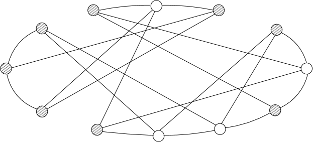
Figure 1: A random graph with 4 sites (open circles) having $z=4$, and 8 sites (filled circles) having $z=3$.

Simulations are performed on a random graph of $N$ sites where $cN$ sites have $z=4$ nearest neighbors, and the rest have $z=3$. A random graph for $z=4$ is constructed as described in reference  dhar and then a fraction of fourth neighbor bonds are removed. Figure (1) illustrates a random graph of 12 sites with 4 sites having $z=4$ and 8 sites having $z=3$. The actual simulations are performed on graphs of size $N>10^{6}$, and $0\leq c\leq 1$. We generate a quenched random-field distribution $\{h_{i}\}$ for a fixed value of $c$ and $\sigma$, and start with a sufficiently negative value of $h$ when all spins are down $\{s_{i}=-1\}$. The applied field $h$ is then increased slowly till some site becomes unstable i.e. it sees a positive local field at its site. At this point, $h$ is kept fixed and the system is updated iteratively till a fixed point is reached i.e. each spin is aligned along the local field at its site. The spins that flip up on the way to the fixed point form a connected cluster, and the number of spins that flip up is the size of the avalanche at $h$. Now $h$ is increased to the next instability in the system, and again the size of the avalanche is calculated as above. The process is repeated till all spins are up and stable. The locus of the fixed points gives the magnetization curve $m(h;\sigma,c)$ in increasing applied field $h$. The magnetization curve is macroscopically smooth but noisy (Barkhausen noise) at a microscopic scale because of the avalanches that separate neighboring fixed points. Our objective is to determine if the magnetization curve has a discontinuity i.e. if two neighboring fixed points are separated by a macroscopic avalanche.

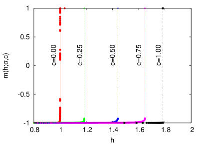
Figure 2: Magnetization $m(h;\sigma,c)$ in increasing field $h$ for $N=10^{8}$, $\sigma=0.50$ and values of $c$ as marked vertically next to each curve.

The value of $h$ where a discontinuity occurs in $m(h;\sigma,c)$, if indeed there is a discontinuity, shifts slightly from one configuration of random fields to another for the same size of the system. Averaging the magnetization over different configurations tends to smoothen the curve and hide the discontinuity. A discontinuity is better seen in a single run of a large system. Figure (2) shows magnetization curves for a single run for $N=10^{8}$, $\sigma=0.5$ and different values of $c$. We choose $\sigma=0.5$ because it is known from earlier work that $m(h;\sigma=0.5,c)$ is continuous for $c=0$ but discontinuous for $c=1$. Therefore for $\sigma=0.5$, there must be a value of $c$ where the behavior changes from smooth to discontinuous. However, it is difficult to read this from figure (2). Each curve in figure (2) seems to have a discontinuity, although the curve for $c=0$ has a slightly different character. With the benefit of an exact solution for $c=0$ we know that the curve will become smooth as the system size is increased beyond $N=10^{8}$. However, deciding a discontinuity by visual inspection is inadequate, and particularly so for locating the critical value $\sigma_{c}$ above which the discontinuity may disappear.

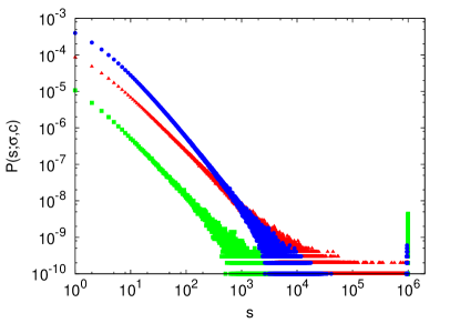
Figure 3: Probability $P(s;\sigma,c)$ of an avalanche of size $s$ along the lower half of the hysteresis loop for $\sigma=0.50$. The data is obtained from avalanches in a system of size $N=10^{6}$, averaged over $10^{4}$ independent configurations of the random field. The figure shows three cases (i) red (triangles) for $c=0$, (ii) blue (circles) for $c=0.5$, and (iii) green (squares) for $c=1$. Theory predicts discontinuous magnetization curves for $c=0.5$ and $c=1$, but continuous for $c=0$.

Another method of analyzing the data is to use the distribution of avalanche sizes  farrow . The probability $P(s;\sigma,c)$ of an avalanche of size $s$ on the trajectory $m(h;\sigma,c)$ is generally a product of two terms: (i) one that decreases exponentially with increasing $s$ and represents microscopic avalanches, and (ii) a delta function peak at a very large value of $s$ representing a macroscopic discontinuity. Figure (3) shows a plot of $\ln{P(s;\sigma=0.5,c)}$ $vs.$ $s$ for $c=0,0.5,1$ respectively. Figure (3) presents the data for $N=10^{6}$, averaged over $10^{4}$ configurations of the random-field distribution. An exact solution for integer $c$ predicts that $m(h;\sigma=0.5,c)$ is continuous for $c=0$, but discontinuous for $c=1$. The motivation behind the plot in figure (3) is to get an indication if the case of $c=0.5$ is more like $c=0$ or $c=1$. Evidently no definite conclusion can be reached in this regard from figure (3). The curve for $c=0.5$ seems to have a mixture of features of $c=0$ and $c=1$; there is an indication of a delta function peak, but there is also a relatively large proportion of small size avalanches which is characteristic of a smooth curve. It is fair to say that figure (3) alone does not give a clear indication of the nature of singularity for $c=0$ or $c=1$, let alone for intermediate values of $c$.

Evidently, finite size effects make it difficult to distinguish between a sharply rising continuous curve and one with a discontinuity. There does not appear to be a numerical method that can differentiate between these two types of curves with certainty. We also tested the ratio $R$ of the largest to the second largest avalanche on the magnetization curve. $R$ should diverge if a discontinuity is present, and therefore it may separate curves with a discontinuity from those without it. The efficacy of this method is rather poor for $\sigma=0.5$ but improves around $\sigma=1$ where it indicates the presence of a discontinuity for all positive values of $c$. However, we omit this analysis here and present an analytic solution of the problem which makes the situation clear.

III Analytic results

As discussed in reference  dhar , the thermodynamic limit of a random graph has the same structure as the deep interior of a Cayley tree. Theoretical analysis is simpler on a Cayley tree because of the absence of loops on it. We are able to adapt the method used in reference  dhar to the present case. A Cayley tree with $z=4$ is shown schematically in figure (3). Initially all spins are kept down. Spins are relaxed starting from the surface of the tree and moving one level at a time towards the root of the tree. Thus spins at level $n+1$ are relaxed keeping their nearest neighbor at level $n$ down. Consider a particular site at level $n$. It has three neighbors at level $n+1$ and one at level $n-1$. Any one of its four neighbors may be missing with probability $1-c$. If the missing neighbor is at level $n-1$, the site in question forms the vertex of a sub-tree which is disconnected from the rest of the tree and therefore does not affect the root of the tree. However, in writing a recursion relation for the relaxation process, we find it convenient to assume that the missing neighbor lies at level $n+1$ only. It amounts to overestimating the presence of $z=4$ sites on the lattice but we correct for it later.

Now we focus on the three sites at level $n+1$ referred above. One of these may be missing with probability $1-c$. If not missing, it may be a $z=4$ site or a $z=3$ site. Let $P^{n+1}_{4}(h)$, and $P^{n+1}_{3}(h)$ be the probability that the spin is up in the two cases respectively. The average probability that the spin at the site is up is equal to $<P^{n+1}(h)>=cP^{n+1}_{4}(h)+(1-c)P^{n+1}_{3}(h)$. It is easy to see that $P^{n}_{4}(h)$ and $P^{n}_{3}(h)$ are given by the recursion relations,

$$P^{n}_{4}(h)=<P^{n+1}(h)>^{3}p_{43}(h)+3<P^{n+1}(h)>^{2}[1-<P^{n+1}(h)>]p_{42}(h)$$

$$+3<P^{n+1}(h)>[1-<P^{n+1}(h)>]^{2}p_{41}(h)+[1-<P^{n+1}(h)>]^{3}p_{40}(h)$$ (3)

$$P^{n}_{3}(h)=<P^{n+1}(h)>^{2}p_{32}(h)+2<P^{n+1}(h)>[1-<P^{n+1}(h)>]p_{31}(h)$$

$$+[1-<P^{n+1}(h)>]^{2}p_{30}(h)$$ (4)

Here, $p_{zm}(h)$, $z=3,4$ and $m\leq z$, is the probability that the random-field at a site with $z$ neighbors is large enough so that the spin at the site can flip up if $m$ of its neighbors are up.

$$p_{zm}(h)=\frac{1}{\sqrt{2\pi\sigma^{2}}}\int_{(z-2m)J-h}^{\infty}dh_{i}\exp{-(h_{i}^{2}/2\sigma^{2})}\hskip 14.22636pt(m\leq z)$$

Equations (3) and (4) lead to fixed points $P^{*}_{4}(h)$ and $P^{*}_{3}(h)$ in the limit $n\rightarrow\infty$. Given that the spin at the root of the tree (i.e. any site in the deep interior of the Cayley tree) is down, the probability that its neighbor is up is given by, $P^{*}(h)=cP^{*}_{4}(h)+(1-c)P^{*}_{3}(h)$. The probability that the spin at the root is up depends on whether the root is a $z=4$ site or a $z=3$ site, and is given respectively by the following equations.

$$p_{4}(h)=[P^{*}(h)]^{4}p_{44}(h)+4[P^{*}(h)]^{3}[1-P^{*}(h)]p_{43}(h)+6[P^{*}(h)]^{2}[1-P^{*}(h)]^{2}p_{42}(h)$$

$$+4[P^{*}(h)][1-P^{*}(h)]^{3}p_{41}(h)+[1-P^{*}(h)]^{4}p_{40}(h)$$ (5)

$$p_{3}(h)=[P^{*}(h)]^{3}p_{33}(h)+3[P^{*}(h)]^{2}[1-P^{*}(h)]p_{32}(h)+3P^{*}(h)[1-P^{*}(h)]^{2}p_{31}(h)$$

$$+[1-P^{*}(h)]^{3}p_{30}(h)$$ (6)

The probability that the spin at the root is up is equal to $p(h)=cp_{4}(h)+(1-c)p_{3}(h)$, and the magnetization per site is equal to $m(h;\sigma,c)=2p(h)-1$. The magnetization per site on $z=3$ and $z=4$ sites is given by $m_{3}(h;\sigma,c)=2p_{3}(h)-1$ and $m_{4}(h;\sigma,c)=2p_{4}(h)-1$ respectively.

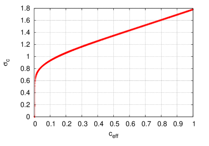
Figure 5: The critical value $\sigma_{c}$ vs. $c$ as obtained from the fixed point equations. The concentration $c$ of $z=4$ sites on the random graph corresponds to $c_{eff}=4c/(3+c)$ on the $x$-axis in the above figure. Critical hysteresis occurs on random graphs only if $\sigma<\sigma_{c}$.

The discontinuity in magnetization is related to a discontinuity in the fixed points $P^{*}_{4}(h)$ and $P^{*}_{3}(h)$ as a function of $h$. Since $P^{*}_{4}(h)$ and $P^{*}_{3}(h)$ are determined by coupled equations, a discontinuity in $P^{*}_{4}(h)$ at $h$ is accompanied by a discontinuity in $P^{*}_{3}(h)$ as well. We focus on their average value $P^{*}(h)=cP^{*}_{4}(h)+(1-c)P^{*}_{3}(h)$. Equations (3) and (4) reveal a critical value $\sigma_{c}$ for each concentration $c$ of $z=4$ sites: $\sigma_{c}$ separates discontinuous from continuous behavior of $P^{*}(h)$ and $m(h;\sigma,c)$. If $\sigma<\sigma_{c}$, $P^{*}(h)$ has three roots in a window of applied field centered at $h=J$. One of these roots is $P^{*}(h)=0.5$ at $h=J$, but this root is unstable. The other two roots are stable and correspond to a discontinuity in $P^{*}(h)$ which jumps up from a value $P^{*}(h)<0.5$ to a higher value $P^{*}(h)>0.5$. This corresponds to a jump in magnetization from a negative to a positive value. The size of the jump reduces as $\sigma$ increases, and vanishes at a non-equilibrium critical point at $\sigma=\sigma_{c}$ and $h=J$. At the critical point the two stable roots for $P^{*}(h)$ merge into each other. We determine $\sigma_{c}$ algebraically by requiring the two stable roots of the fixed point equation become a double root. The result is depicted in figure (5). It predicts that the discontinuity in $m(h;\sigma,c)$ occurs for all values of $c$ greater than zero and $\sigma<\sigma_{c}$; $\sigma_{c}$ decreases with decreasing $c$. For $\sigma>\sigma_{c}$, the magnetization curve is smooth.

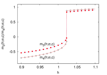
Figure 7: Magnetization $m_{3}(h;\sigma,c)$ and $m_{4}(h;\sigma,c)$ for $c=0.75,\sigma=1.5$ near a discontinuity. Theoretical expressions have been superimposed on the simulation data from a single run ($N=10^{7}$).

Before comparing the theoretical result with numerical simulations, we make a correction to which we alluded earlier in this section. The recursion relations on the Cayley tree assume that a $z=3$ site at level $n$ is necessarily connected to its neighbor at level $n-1$. This overestimates the concentration of $z=4$ sites at level $n-1$ by a fraction $(1-c)/4$, i.e. the fraction of $z=4$ sites at level $n-1$ becomes $c(1+(1-c)/4)$. The correction propagates all the way to the deep interior of the tree. The effective concentration of $z=4$ sites in the vicinity of the central site becomes $c_{eff}=c(1+r+r^{2}+r^{3}+\ldots)$ where $r=(1-c)/4$. Summing the geometric series we get, $c_{eff}=4c/(3+c)$. Thus simulations on a random graph with a fraction $c$ of $z=4$ sites should match the theoretical result for $c_{eff}$. This is indeed the case. A few selected comparisons are shown in figure (6) and figure (7). Figure (6) shows magnetization $m(h;\sigma,c)$ for $c=0.1,\sigma=0.9$ and $c=0.9,\sigma=1.6$ near a discontinuity. Corresponding theoretical expressions have been superposed on the simulation results and the two fit each other quite well. The curve with the discontinuity closer to $h=J$ is for $c=0.1$, and the other for $c=0.9$. The critical values of $\sigma$ for $c=0.1$ and $c=0.9$ are $\sigma_{c}=0.93$ and $\sigma_{c}=1.69$ respectively. Since the simulations are for $\sigma<\sigma_{c}$ but close to $\sigma_{c}$, they show discontinuity at $h>J$ but close to it. Figure (7) shows $m_{3}(h;\sigma,c)$ and $m_{4}(h;\sigma,c)$, the magnetization per site on $z=3$ and $z=4$ sites respectively for $c=0.75$ and $\sigma=1.5$ ($\sigma_{c}=1.56$). Again the corresponding theoretical expressions have been superimposed on the simulations and the fit is quite good as may be expected.

IV Discussion

The work presented above extends the treatment of critical hysteresis on Bethe lattices of integer coordination number to lattices with a fractional coordination number. It is significant from two points of view. The first point concerns the question of a lower critical coordination number $z_{l}$ vs. a lower critical dimension $d_{l}$. The existence of a non-equilibrium critical point is decided by $z_{l}$ rather than $d_{l}$. Earlier work suggested $z_{l}=4$, but the present result shows $z_{l}>3$. The physical significance of $z_{l}$ is not very clear at present. Mathematically, a discontinuity in $m(h;\sigma,c)$ occurs when $m(h;\sigma,c)$ has an ”$s$-shape”. An $s$-shape requires three solutions for $m(h;\sigma,c)$ for the same value of the applied field $h$ in some range of $h$. The middle part of the $s$-shaped curve on which $m(h;\sigma,c)$ decreases with increasing $h$ is physically unstable causing the magnetization to jump over it. Earlier work examined only integer values of $z$ and found $z=4$ to be the smallest value of $z$ for which $m(h;\sigma,c)$ could have three solutions. Somewhat surprisingly, this result for the Bethe lattice seems to apply also to several periodic lattices of integer coordination number, irrespective of the dimensionality of space $d$ in which the lattice is embedded. We have examined fractional coordination numbers and find $z_{l}>3$. Of course, the coordination number $z$ of a lattice site is necessarily an integer. We constructed random graphs with a mixture of sites with $z=3$ and $z=4$ so that the average coordination number $z$ lies between $3$ and $4$. Random graphs are excellent representations of a Bethe lattice or the deep interior of a Cayley tree. We studied the problem numerically on random graphs, but analytically on a Cayley tree. The numerical results fit corresponding theoretical expressions quite well. After an analytic solution is found, one may think the role of numerical work is essentially to check the solution. However, we have presented a brief account of our numerical effort to emphasize its difficulty in deciding the question of a true discontinuity in the magnetization. Methods which work on lattices of a uniform coordination number become less efficient when $z$ is disordered. Even on random graphs, it is hard to draw clear conclusions unless aided by analytical results. Since it is extremely difficult to obtain exact solutions on periodic lattices, search for better numerical methods has to continue.

The second point is that lattices with a mixed coordination number are quite common and important in the field of amorphous solids  mitra . In magnetism, the coordination number of a site determines the exchange and the anisotropy field at the site and therefore the predominant nature of the spin at the site i.e. discrete or continuous. This in turn affects the relaxation rate of the spin, and the shape of the hysteresis loop  kharwanlang . Similar effects are also important in molecular magnetism and its industrial applications  zadrozny . Thus the work presented here may be useful in understanding non-equilibrium phase transitions in a wider class of disordered materials and their applications.

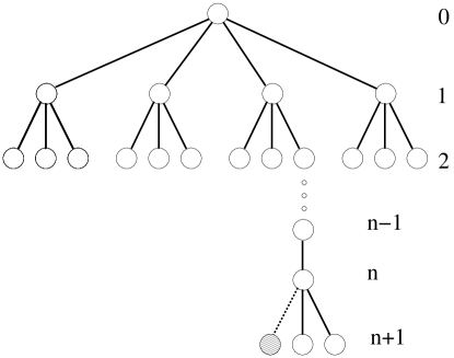
Figure 4: A Cayley tree of mixed coordination $z=3$ and $z=4$. A dark circle at level $n+1$ represents a $z=3$ site. Any of its four neighbors may be missing with probability $1/4$ but the recursion relations assume that the missing neighbor does not lie at level $n$. This overestimates the concentration of $z=4$ sites at level $n$. A fraction $c$ of $z=4$ sites on a random graph corresponds to a fraction $c_{eff}=4c/(3+c)$ in the deep interior of the Cayley tree (see text).

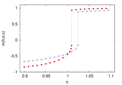
Figure 6: Magnetization $m(h;\sigma,c)$ for $c=0.1,\sigma=0.9$ (red/filled circles) and $c=0.9,\sigma=1.6$ (blue/open circles) near a discontinuity. Corresponding theoretical expressions have been superimposed on the simulation data for a single configuration of random-field for a system of size $N=10^{7}$.

References

- (1) J P Sethna, K A Dahmen, S Kartha, J A Krumhansl, B W Roberts, and J D Shore, Phys Rev Lett 70, 3347 (1993).
- (2) J P Sethna, K A Dahmen, and C R Myers, Nature 410, 242 (2001).
- (3) K Dahmen and J P Sethna, Phys Rev Lett 71, 3222(1993); K A Dahmen and J P Sethna, Phys Rev B 53, 14872 (1996).
- (4) O Perkovic, K Dahmen, and J P Sethna, Phys Rev Lett 75, 4528 (1995); O Percovic, K.A Dahmen and J.P Sethna, Phys. Rev. B 59, 6106(1999); O Percovic,K A Dahmen and J P Sethna, arXiv:cond-mat/9609072 v1.
- (5) J P Sethna, K A Dahmen, O Perkovic, in The Science of Hysteresis edited by G Bertotti and I Mayergoyz (Academic Press, Amsterdam, 2006).
- (6) Y Imry and S.-k. Ma, Phys Rev Lett 35, 1399 (1975).
- (7) M Aizenman and J Wehr, Phys Rev Lett 62, 2503 (1989); 64, 1311 (1990).
- (8) L Onsager, Phys Rev 65, 117 (1944).
- (9) P Shukla, Prog Theo Phys 96, 69-80 (1996); P Shukla, Phys Rev E 63, 27102 (2001).
- (10) D.Spasojevic, S. Janicevic and M.Knezevic, Phys. Rev. Lett, 106,175701(2011); Phys Rev E84, 051119 (2011).
- (11) D Thongjaomayum and P.Shukla, Phys Rev E 88, 042138 (2013).
- (12) S Sabhapandit, D Dhar, and P Shukla, Phys Rev Lett 88, 197202 (2002).
- (13) D Dhar, P Shukla, and J P Sethna, J Phys A30, 5259 (1997), and references therein.
- (14) L Kurbah, D Thongjaomayum and P.Shukla, Phys Rev E 91, 012131 (2015).
- (15) C. L. Farrow, P. Shukla, and P. M. Duxbury, J. Phys. A: Math. Theor. 40, F581 (2007); P. Shukla, Pramana 71, 319 (2008).
- (16) Physics of Structurally Disordered Solids, ed. S Mitra, Springer Science (2013).
- (17) R S Kharwanlang and P Shukla, Phys Rev E 85, 011124 (2012), and references there in.
- (18) J M Zadrozny et. al., Chem. Sci. 4, 125 (2013).