Random Forests for Big Data

Abstract

Big Data is one of the major challenges of statistical science and has numerous consequences from algorithmic and theoretical viewpoints. Big Data always involve massive data but they also often include online data and data heterogeneity. Recently some statistical methods have been adapted to process Big Data, like linear regression models, clustering methods and bootstrapping schemes. Based on decision trees combined with aggregation and bootstrap ideas, random forests were introduced by Breiman in 2001. They are a powerful nonparametric statistical method allowing to consider in a single and versatile framework regression problems, as well as two-class and multi-class classification problems. Focusing on classification problems, this paper proposes a selective review of available proposals that deal with scaling random forests to Big Data problems. These proposals rely on parallel environments or on online adaptations of random forests. We also describe how related quantities – such as out-of-bag error and variable importance – are addressed in these methods. Then, we formulate various remarks for random forests in the Big Data context. Finally, we experiment five variants on two massive datasets (15 and 120 millions of observations), a simulated one as well as real world data. One variant relies on subsampling while three others are related to parallel implementations of random forests and involve either various adaptations of bootstrap to Big Data or to “divide-and-conquer” approaches. The fifth variant relates on online learning of random forests. These numerical experiments lead to highlight the relative performance of the different variants, as well as some of their limitations.

1 Introduction

1.1 Statistics in the Big Data world

Big Data is one of the major challenges of statistical science and a lot of recent references start to think about the numerous consequences of this new context from the algorithmic viewpoint and for the theoretical implications of this new framework (see [1, 2, 3]). Big Data always involve massive data but they also often include data streams and data heterogeneity (see [4] for a general introduction), often characterized by the fact that data are frequently not structured data, properly indexed in a database and that simple queries cannot be easily performed on such data. These features lead to the famous three V (Volume, Velocity and Variety) highlighted by the Gartner, Inc., the advisory company about information technology research . In the most extreme situations, data can even have a too large size to fit in a single computer memory. Then data are distributed among several computers. For instance, Thusoo et al. [5] indicate that Facebook^© had more than 21PB of data in 2010. Frequently, the distribution of such data is managed using specific frameworks dedicated to shared computing environments such as Hadoop.

For statistical science, the problem posed by this large amount of data is twofold: first, as many statistical procedures have devoted few attention to computational runtimes, they can take too long to provide results in an acceptable time. When dealing with complex tasks, such as learning of a prediction model or complex exploratory analysis, this issue can occur even if the dataset would be considered of a moderate size for other (simpler tasks). Also, as pointed out in [6], the notion of Big Data depends itself on the available computing resources. This is especially true when relying on the free statistical software R [7], massively used in the statistical community, which capabilities are strictly limited by RAM. In this case, data can be considered as “large” if their size exceeds 20% of RAM and as “massive” if it exceeds 50% of RAM, because this amount of data strongly limits the available memory for learning the statistical model itself. As pointed out in [3], in the near future, statistics will have to deal with problems of scale and computational complexity to remain relevant. In particular, the collaboration between statisticians and computer scientists is needed to control runtimes that will maintain the statistical procedures usable on large-scale data while ensuring good statistical properties.

Recently, some statistical methods have been adapted to process Big Data, including linear regression models, clustering methods and bootstrapping schemes (see [8] and [9] for recent reviews and useful references). The main proposed strategies are based on i) subsampling [10, 11, 12, 13, 14], ii) divide and conquer approaches [15, 16, 17], which consist in splitting the problem into several smaller problems and in gathering the different results in a final step, iii) algorithm weakening [18], which explicitly treats the trade-off between computational time and statistical accuracy using a hierarchy of methods with increasing complexity, iv) online updates [19, 20], which update the results with sequential steps, each having a low computational cost. However, only a few papers really address the question of the difference between the “small data” standard framework compared to the Big Data in terms of statistical accuracy. Noticeable exceptions are the article of Kleiner et al. [12] who prove that their “Bag of Little Bootstraps” method is statistically equivalent to the standard bootstrap, the article of Chen and Xie [16] who demonstrate asymptotic equivalence to their “divide-and-conquer” based estimator with the estimator based on all data in the setting of regression and the article of Yan et al. [11] who show that the mis-clustering rate of their subsampling approach, compared to what would have been obtained with a direct approach on the whole dataset, converges to zero when the subsample size grows (in an unsupervised setting).

1.2 Random forests and Big Data

Based on decision trees and combined with aggregation and bootstrap ideas, random forests (abbreviated RF in the sequel), were introduced by Breiman [21]. They are a powerful nonparametric statistical method allowing to consider regression problems as well as two-class and multi-class classification problems, in a single and versatile framework. The consistency of RF has recently been proved by Scornet et al. [22], to cite the most recent result. On a practical point of view, RF are widely used (see [23, 24] for recent surveys) and exhibit extremely high performance with only a few parameters to tune. Since RF are based on the definition of several independent trees, it is thus straightforward to obtain a parallel and faster implementation of the RF method, in which many trees are built in parallel on different cores. In addition to the parallel construction of a lot of models (the trees of a given forest) RF include intensive resampling and, it is natural to think about using parallel processing and to consider adapted bootstrapping schemes for massive online context.

Even if the method has already been adapted and implemented to handle Big Data in various distributed environments (see, for instance, the libraries Mahout or MLib, the latter for the distributed framework “Spark”, among others), a lot of questions remain open. In this paper, we do not seek to make an exhaustive description of the various implementations of RF in scalable environments but we will highlight some problems posed by the Big Data framework, describe several standard strategies that can be use for RF and describe their main features, drawbacks and differences with the original approach. We finally experiment five variants on two massive datasets (15 and 120 millions of observations), a simulated one as well as real world data. One variant relies on subsampling while three others are related to parallel implementations of random forests and involve either various adaptations of bootstrap to Big Data or to “divide-and-conquer” approaches. The fifth variant relates to online learning of RF.

Since the free statistical software R [7], is de facto the esperanto in the statistical community, and since the most widely used programs for designing random forests are also available in R, we have adopted it for numerical experiments as much as possible. More precisely, the R package randomForest, implementing the original RF algorithm using Breiman and Cutler’s Fortran code, contains many options together with a detailed documentation. It has then been used in almost all experiments. The only exception is for online RF for which no implementation in R is available. We then use a python library, as an alternative tool in order to provide the means to compare this approach to the alternative Big Data variants.

The paper is organized as follows. After this introduction, we briefly recall some basic facts about RF in Section 2. Then, Section 3 is focused on strategies for scaling random forests to Big Data: some proposals about RF in parallel environments are reviewed, as well as a description of online strategies. The section includes a comparison of the features of every method and a discussion about the estimation of the out-of-bag error in these methods. Section 4 is devoted to numerical experiments on two massive datasets, an extensive study on a simulated one and an application to a real world one. Finally, Section 5 collects some conclusions and discusses two open perspectives.

2 Random Forests

Denoting by $L=\{(x_{1},y_{1}),\ldots,(x_{n},y_{n})\}$ a learning set of independent observations of the random vector $(X,Y)$, we distinguish $X=(X^{1},...,X^{p})$ where $X\in{R}^{p}$ is the vector of the predictors (or explanatory variables) from $Y\in\mathcal{Y}$ the explained variable, where $Y$ is either a class label for classification problems or a numerical response for regression ones. A classifier $s$ is a mapping $s:{R}^{p}\rightarrow\mathcal{Y}$ while the regression function appears naturally to be the function $s$ when we suppose that $Y=s(X)+\varepsilon$ with $E[\varepsilon|X]=0$. RF provide estimators of either the Bayes classifier, which minimizes the classification error $P(Y\neq s(X))$ or the regression function (see [25, 26] for further details on classification and regression problems). RF are a learning method for classification and regression based on the CART (Classification and Regression Trees) method defined by Breiman et al. [27]. The left part of Figure 1 provides an example of classification tree. Such a tree allows to predict the class label corresponding to a given $x$-value by simply starting from the root of the tree (at the top of the left part of the figure) and by answering the questions until a leaf is reached. The predicted class is then the value labeling the leaf. Such a tree is a classifier $s$ which allows to predict a $y$-value for any given $x$-value. This classifier is the function which is piecewise constant on the partition described in the right part of Figure 1. Note that splits are parallel to the axes defined by the original variables leading to an additive model.

Figure 1: Left: a classification tree allowing to predict the class label corresponding to a given $x$-value. Right: the associated partition of the predictor space.

While CART is a well-known way to design optimal single trees by performing first a growing step and then a pruning one, the principle of RF is to aggregate many binary decision trees coming from two random perturbation mechanisms: the use of bootstrap samples (obtained by randomly selecting $n$ observations with replacement from learning set $L$) instead of the whole sample $L$ and the construction of a randomized tree predictor instead of CART on each bootstrap sample. For regression problems, the aggregation step consists in averaging individual tree predictions, while for classification problems, it consists in performing a majority vote among individual tree predictions. The construction is summarized in Figure 2.

Figure 2: RF construction scheme: starting from the dataset (left of the figure), generate bootstrap samples (by randomly selecting $n$ observations with replacement from learning set $L$) and learn corresponding randomized binary decision trees. Finally aggregate them.

However, trees in RF have two main differences with respect to CART trees: first, in the growing step, at each node, a fixed number of input variables are randomly chosen and the best split is calculated only among them, and secondly, no pruning is performed.

In the next section, we will explain that most proposals made to adapt RF to Big Data often consider the original RF proposed by Breiman as an object that simply has to be mimicked in the Big Data context. But we will see, later in this article, that alternatives to this vision are possible. Some of these alternatives rely on other ways to resample the data and others are based on variants in the construction of the trees.

We will concentrate on the prediction performance of RF, focusing on out-of-bag (OOB) error, which allows to quantify the variable importance (VI in the sequel). The quantification of the variable importance is crucial for many procedures involving RF, e.g., for ranking the variables before a stepwise variable selection strategy (see [28]). Notations used in this section are given in Table 1

notation	used for
$n$	number of observations in dataset
$Q$	number of trees in the RF classifier
$t$	a tree in the RF classifier
OOBt	set of observations out-of-bag for the tree $t$
errTreet	misclassification rate for observations in OOBt made by $t$
$\widetilde{\textrm{errTree}}_{t}^{j}$	misclassification rate for observations OOB for $t$
	after a random permutations of values of $X^{j}$
$\hat{y}_{i}$	OOB prediction of observation $x_{i}$
	(aggregation of predictions made by trees $t$ such that $i\in\textrm{OOB}_{t}$)
errForest	OOB misclassification rate for the RF classifier
VI($X^{j}$)	Variable importance of $X^{j}$

Table 1: Notations used in Section 2.

For each tree $t$ of the forest, consider the associated $\mbox{OOB}_{t}$ sample (composed of data not included in the bootstrap sample used to construct $t$). The OOB error rate of the forest is defined, in the classification case, by:

$$\mbox{errForest}=\frac{1}{n}\mathrm{Card}\left\{i\in\{1,\ldots,n\}\>|\>y_{i}\neq\hat{y_{i}}\right\}$$ (1)

where $\hat{y_{i}}$ is the most frequent label predicted by trees $t$ for which observation $i$ is in the associated $\mbox{OOB}_{t}$ sample.

Denote by $\mbox{errTree}_{t}$ the error (misclassification rate for classification) of tree $t$ on its associated $\mbox{OOB}_{t}$ sample. Now, randomly permute the values of $X^{j}$ in $\mbox{OOB}_{t}$ to get a perturbed sample and compute $\widetilde{\mbox{errTree}_{t}}^{j}$, the error of tree $t$ on the perturbed sample. Variable importance of $X^{j}$ is then equal to:

$$\mbox{VI}(X^{j})=\frac{1}{Q}\sum_{t}(\widetilde{\mbox{errTree}_{t}}^{j}-\mbox{errTree}_{t})\$$

where the sum is over all trees $t$ of the RF and $Q$ denotes the number of trees of the RF.

3 Scaling random forests to Big Data

This section discusses the different strategies that can be used to scale random forest to Big Data: the first one is subsampling, denoted by sampRF in the sequel. Then, four parallel implementations of random forests (parRF, moonRF, blbRF and dacRF), relying on standard parallelization, adaptation of bootstraping schemes to Big Data or on a divide-and-conquer approach, are also presented. Finally, a different (and not equivalent) approach based on the online processing of data is also described, onRF. All these variants are compared to the original method, seqRF, in which all bootstrap samples and trees are built sequentially. The names of the different methods and references to the sections in which they are discussed are summarized in Table 2.

short name	full name	described in	relies on
seqRF	sequential RF	2	original method
sampRF	sampling RF	3.1	subsampling
parRF	parallel RF	3.2	parallelization
moonRF	$m$-out-of-$n$ RF	3.2.1	Big Data bootstrap
blbRF	Bag of Little Bootstraps RF	3.2.1	Big Data bootstrap
dacRF	divide-and-conquer RF	3.2.2	divide-and-conquer
onRF	online RF	3.3	online learning

Table 2: Names and references of the different variants of RF described in this article.

In addition, the section will use the following notations: RF will denote the random forest method (in a generic sense) or the final random forest classifier itself, obtained from the various approaches described in this section. The number of trees in the final classifier RF is denoted by $Q$, $n$ is the number of observations of the original dataset and, when a subsample is taken in this dataset (either with or without replacement), it is denoted by $\tau_{l}$ ($l$ identifies the subsample when several subsamples are used) and its size is usually denoted by $m$. When different processes are run in parallel, the number of processes is denoted by $K$. Depending on the method, this can lead to learn smaller RF with $q<Q$ trees that are denoted by $\textrm{RF}_{l}^{(q)}$, in which $l$ is an index that identifies the RF. The notation $\cup_{l=1}^{K}\textrm{RF}_{l}^{(q)}$ will be used for the classifier obtained from the aggregation of $K$ RF with $q$ trees each into a RF with $qK$ trees. Similarly, $t_{l}$ or $t_{ll^{\prime}}$ denote a tree, identified by the index $l$ or by two indices, $l$ and $l^{\prime}$, when required, and $\cup_{l=1}^{q}t_{l}$ denotes the random forest obtained from the aggregation of the $q$ trees $t_{1}$, …, $t_{q}$. Additional notations used in this section are summarized in Table 3.

notation	used for
$\tau_{l}$	subsample of the observations in the dataset
$m$	number of observations in subsamples
RF	final random forest classifier
$Q$	number of trees in the final random forest classifier
$K$	number of processes run in parallel
$q$	number of trees in intermediate (smaller) random forests
$\textrm{RF}_{l}^{(q)}$	RF number $l$ with $q$ trees
$\cup_{l=1}^{K}\textrm{RF}_{l}^{(q)}$	aggregation of $K$ RF with $q$ trees in a single classifier
$t_{l}$ or $t_{ll^{\prime}}$	tree identified by the index $l$ or by indices $l$ and $l^{\prime}$
$\cup_{l=1}^{q}t_{l}$	aggregation of $q$ trees in an RF classifier

Table 3: Notations used in Section 3.

3.1 Sub-sampling RF (sampRF)

Meng [14] points the fact that using all data is probably not required to obtain accurate estimations in learning methods and that sampling approaches is an important approach to deal with Big Data. The natural idea behind sampling is to simply subsample $m$ observations out of $n$ without replacement in the original sample (with $m\ll n$) and to use the original algorithm (either seqRF or the parallel implementation, parRF, described in Section 3.2) to process this subsample. This method is illustrated in Figure 3.

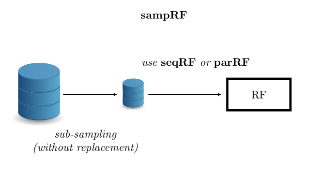
Figure 3: Sub-sampling RF (sampRF): $m$ observations out of $n$ are randomly selected without replacement and the original RF algorithm (seqRF) or its parallel version (parRF) described in Section 3.2 are used to obtain a final random forest with $Q$ trees.

Subsampling is a natural method for statisticians and it is appealing since it strongly reduces memory usage and computational efforts. However, it can lead to serious biases if the subsample is not carefully designed. More precisely, the need to control the representativeness of the subsampling is crucial. Random subsampling are usually adequate for such tasks, providing the fact that the sampling fraction is large enough. However, in the Big Data world, datasets are frequently not structured and indexed. In this situation, random subsampling can be a difficult task (see [14] for a discussion on this point and a description of a parallel strategy to overcome this problem). Section 4 provides various insights on the efficiency of subsampling, on the effect of the sampling fraction and on the representativeness of the subsample on the accuracy of the obtained classifier. The next section investigates approaches which try to make use of a wider proportion of observations in the dataset using efficient computational strategies.

3.2 Parallel implementations of random forests

As pointed in the introduction, RF offer a natural framework for handling Big Data. Since the method relies on bootstraping and independant construction of many trees, it is naturally suited for parallel computation. Instead of building all $Q$ bootstrap samples and trees sequentially as in seqRF, bootstrap samples and trees (or sets of a small number of bootstrap samples and trees) can be built in parallel. In the sequel, we will denote by parRF the approach in which $K$ processes corresponding to the learning of a forest with $q=\frac{Q}{K}$ trees each are processed in parallel. seqRF and parRF implementations are illustrated in Figure 4 (left and right, respectively). Using the parRF approach, one can hope for a computational time factor decrease of approximately $K$ between seqRF and parRF.

Figure 4: Sequential (left) and parallel (right) implementations of the standard RF algorithm. RF is the final random forest with $Q$ trees. parRF builds $K$ small random forests, $\textrm{RF}^{(q)}_{l}$, with $q=\frac{Q}{K}$ trees each, using $K$ processes run in parallel.

However, as pointed in [12], since the expected size of a bootstrap sample built from $\{1,\ldots,n\}$ is approximately $0.63n$, the need to process hundreds of such samples is hardly feasible in practice when $n$ is very large. Moreover, in the original algorithm from [21], the trees that composed the forest are fully developed trees, which means that the trees are grown until every terminal node (leaf) is perfectly homogeneous regarding the values of $Y$ for the observations that fall in this node. When $n$ is large, and especially in the regression case, this leads to very deep trees which are all computationally very expensive and even difficult to use for prediction purpose. However, as far as we know, no study addresses the question of the impact of controlling and/or tuning the maximum number of nodes in the forest’s trees.

The next subsection presents alternative solutions to address the issue of large size bootstrap samples while relying on the natural parallel background of RF. More precisely, we will discuss alternative bootstrap schemes for RF ($m$-out-of-$n$ bootstrap RF, moonRF, and Bag of Little Bootstraps RF, blbRF) and divide-and-conquer approach, dacRF. A last subsection will describe and comment on the mismatches of each of these approaches with the standard RF method, seqRF or parRF.

3.2.1 Alternative bootstrap schemes for RF (moonRF and blbRF)

To avoid selecting only some of the observations in the original big dataset as it is done in sampRF (Figure 3), some authors have focused on alternative bootstrap schemes aiming at reducing the number of different observations of each bootstrap samples. [29] propose the $m$-out-of-$n$ bootstrap that consists in building bootstrap samples with only $m$ observations taken without replacement in $\{1,\ldots,n\}$ (for $m\ll n$). This method is illustrated in Figure 5.

Figure 5: $m$-out-of-$n$ RF (moonRF): $Q$ samples without replacement with $m$ observations out of $n$ are randomly built in parallel and a tree is learned from each of these samples. The $Q$ trees are then aggregated to obtain a final random forest with $Q$ trees.

Initially designed to address the computational burden of standard bootstrapping, the method performance is strongly dependent on a convenient choice of $m$ and the data-driven scheme proposed in [30] for the selection of $m$ requires to test several different values of $m$ and eliminates computational gains.

More recently, an alternative to $m$-out-of-$n$ bootstrap called “Bag of Little Bootstraps” (BLB) has been described in [12]. This method aims at building bootstrap samples of size $n$, each one containing only $m\ll n$ different observations. The size of the bootstrap sample is the classical one ($n$), thus avoiding the problem of the bias involved by $m$-out-of-$n$ bootstrap methods. The approach is illustrated in Figure 6.

Figure 6: Bag of Little Bootstraps RF (blbRF). In this method, a subsampling step, performed $K$ times in parallel, is followed by an oversampling step which aims at building $q$ trees for each subsample, all obtained from a bootstrap sample of size $n$ of the original data. All the trees are then gathered into a final forest RF.

It consists in two steps: in a first step, $K$ subsamples, $(\tau_{l})_{l=1,\ldots,K}$, are obtained, with $m$ observations each, that are taken randomly without replacement from the original observations. In a second step, each of these subsamples is used to obtain a forest, RF${}^{(q)}_{l}$ with $q=\frac{Q}{K}$ trees. But instead of taking bootstrap samples from $\tau_{l}$, the method uses over-sampling and, for all $i\in\tau_{l}$, computes weights, $n_{i}^{l}$, from a multinomial distribution with parameters $n$ and $\frac{1}{m}\mathbf{1}_{m}$, where $\mathbf{1}_{m}$ is a vector with $m$ entries equal to 1. These weights satisfy $\sum_{i\in\tau_{l}}n_{i}^{l}=n$ and a bootstrap sample of the original dataset is thus obtained by using $n_{i}^{l}$ times each observation $i$ in $\tau_{l}$. For each $\tau_{l}$, $q$ such bootstrap samples are obtained to build $q$ trees. These trees are aggregated in a random forest RF${}^{(q)}_{l}$. Finally, all these (intermediate) random forests with $q$ trees are gathered together in a forest with $Q=qK$ trees. The processing of this method is thus simplified by a smart weighting scheme and is manageable even for very large $n$ because all bootstrap samples contain only a small number (at most $m$) of unique observations from the original data set. The number $m$ is typically of the order $n^{\gamma}$ for $\gamma\in[0.5,1]$, which can be very small compared to the typical number of observations (about $0.63n$) of a standard bootstrap sample. Interestingly, this approach is well supported by theoretical results because the authors of [12] prove its equivalence with the standard bootstrap method.

3.2.2 Divide-and-conquer RF (dacRF)

Standard alternative to deal with massive datasets while not using subsampling is to rely on a “divide-and-conquer” strategy. The large problem is divided into simpler subproblems and the solutions are aggregated together to solve the original problem. The approach is illustrated in Figure 7: the data are split into small sub-samples, or chunks, of data, $(x_{i},y_{i})_{i\in\tau_{l}}$, with $\cup_{l}\tau_{l}=\{1,\ldots,n\}$ and $\tau_{l}\cap\tau_{l^{\prime}}=\emptyset$.

Figure 7: divide-and-conquer RF (dacRF). In this method, the original dataset is partitionned into $K$ subsets. A random forest with $q$ trees is built from each of the subsets and all the forests are finally aggregated in a final forest, RF.

Each of these data chunks is processed in parallel and yields to the learning of an intermediate RF having a reduced number of trees. Finally, all these forests are simply aggregated together to define the final RF.

As indicated in [17], this approach is the standard MapReduce version of RF, implemented in the Apache${}^{\textrm{\tiny TM}}$ library Mahout. MapReduce is a method that proceeds in two steps: in a first step, called the Map step, the data set is split into several smaller chunks of data, $(x_{i},y_{i})_{i\in\tau_{k}}$, with $\cup_{k}\tau_{k}=\{1,\ldots,n\}$ and $\tau_{k}\cap\tau_{k^{\prime}}=\emptyset$, each one being processed by a separate core. These different Map jobs are independent and produce a list of couples of the form $(\mbox{key},\mbox{value})$, where “key” is a key indexing the data that are contained in “value”. In RF case, the output key is always equal to 1 and the output value is the forest learned on the corresponding chunk. Then, in a second step, called the Reduce step, each reduce job proceeds all the outputs of the Map jobs that correspond to a given key value. This step is skipped in RF case since the output of the different Map jobs are simply aggregated together to produce the final RF. The MapReduce paradigm takes advantage of the locality of data to speed the computation. Each Map job usually processes the data stored in a close proximity to its computational unit. As discussed in the next section and illustrated in Section 4.3, this can yield to biases in the resulting RF.

3.2.3 Mismatches with original RF

In this section, we want to stress the differences between the previously proposed parallel solutions and the original algorithm. Two methods will be said “equivalent” when they would provide similar results when used on a given dataset, up to the randomness in bootstrap sampling. For instance, seqRF and parRF are equivalent since the only difference between the two methods are the sequential or parallel learning of the trees. sampRF and dacRF are not equivalent to seqRF and are both strongly dependent on the representativity of the dataset. This is the standard issue encountered in survey approaches for sampRF but it is also a serious limitation to dacRF even if this method uses all observations. Indeed, if data are thrown in the different chunks with no control on the representativity of the subsamples, data chunks might well be specific enough to produce very heterogeneous forests: there would be no meaning in simply averaging all those trees together to make a global prediction. This is especially an issue when using the standard MapReduce paradigm since, as noted by Laptev et al. [13], data are rarely ordered randomly in the Big Data world. On the contrary, items are rather clustered on some particular attributes are often placed next to each other on disk and the data locality property of MapReduce thus leads to very biased data chunks.

Moreover, as pointed out by Kleiner et al. [12], another limit of sampRF and dacRF but also of moonRF comes from the fact that each forest is built on a bootstrap sample of size $m$. The success of $m$-out-of-$n$ bootstrap samples is highly conditioned on the choice of $m$: [29] reports results for $m$ of order $\mathcal{O}(n)$ for successful $m$-out-of-$n$ bootstrap. Bag of Little Bootstraps is an appealing alternative since the bootstrap sample size is the standard one ($n$). Moreover, [12] demonstrate a consistency result of the bootstrap estimation in their framework for $m=\mathcal{O}(\sqrt{n})$ and $K\sim\frac{n}{m}$ (when $n$ tends to $+\infty$).

In addition, some important features of all these approaches are summarized in Table 4. A desirable property for a high computational efficiency is that the number of different observations in bootstrap samples is as small as possible.

	can be computed	bootstrap	expected nb of
	in parallel	sample size	$\neq$ obs. in
			bootstrap samples
seqRF	yes	$n$	$0.63n$
parRF	(parRF)
sampRF	yes but	$m$	$0.63m$
	not critical
moonRF	yes	$m$	$m$
blbRF	yes	$n$	$m\left[1-\left(\frac{m-1}{m}\right)^{n}\right]$
dacRF	yes	$\frac{n}{K}$	$0.63\frac{n}{K}$

Table 4: Summary of the main features in the variants of the random forest algorithm (excluding online RF, onRF).

3.2.4 Out-of-bag error and variable importance measure

OOB error and VI are important diagnostic tools to help the user understand the forest accuracy and to perform variable selection. However, these quantities may be unavailable directly (or in a standard manner) in the RF variants described in the previous sections. This comes from the fact that sampRF, moonRF and blbRF use a prior subsampling step of $m$ observations. The forest (or the subforests) based on this subsample has not a direct access to the remaining $n-m$ observations that are always out-of-bag and should, in theory, be considered for OOB computation. In general, OOB error (and thus VI) cannot be obtained directly while the forest is trained. A similar problem occurs for dacRF in which all forests based on a given chunk of data are unaware of data the other chunks. In dacRF, it can even be memory costly to record which data have been used in each chunk to obtain OOB afterwards. Moreover, even in the case where this information is available, all RF alternatives presented in the previous sections, sampRF, moonRF, blbRF and dacRF, require to obtain the predictions for approximately $n-rm$ OOB observations (with $r=0.63$ for sampRF and dacRF, $r=1$ for moonRF and $r=1-\left(\frac{m-1}{m}\right)^{n}$ for blbRF) for all trees, which can be a computationally extensive task.

In this section, we present a first approximation of OOB error that can naturally be designed for sampRF and dacRF, and a second approximation for moonRF and blbRF. Additional notations used in this section are summarized in Table 5.

notation	used for
$K$	number of subsamples
	(equivalent to the number of processes run in parallel here)
$q$	number of trees in intermediate (smaller) random forests
$\hat{y}_{i}^{l}$	OOB prediction for observation $i\in\tau_{l}$ by forest obtained from $\tau_{l}$
errForestl	OOB error of RF${}_{l}^{(q)}$ restricted to $\tau_{l}$
$\hat{y}_{i}^{-l}$	prediction for observation $i\in\tau_{l}$ by forests (RF${}^{(q)}_{l^{\prime}})_{l^{\prime}\neq l}$
BDerrForest	approximation of OOB in sampRF, blbRF, moonRF and dacRF

Table 5: Notations used in Section 3.2.4.

OOB error approximation for sampRF and dacRF

As previously, $(\tau_{l})_{l=1,\ldots,K}$ denote the subsamples of data, each of size $m$, used to build independent forests in parallel (with $K=1$ for sampRF). Using each of these samples, a forest with $Q$ (sampRF) or $q=\frac{Q}{K}$ (dacRF) trees is defined, for which an OOB prediction, restricted to observations in $\tau_{l}$, can be calculated: $\hat{y}_{i}^{l}$ is obtained by a majority vote on the trees of the forest built from a bootstrap sample of $\tau_{l}$ for which $i$ is OOB.

An approximation of the OOB error of the forest learned from sample $\tau_{l}$ can thus be obtained with $\mbox{errForest}^{l}=\frac{1}{m}\textrm{Card}\left\{i\in\tau_{l}|y_{i}\neq\hat{y}_{i}^{l}\right\}$. This yields to the following approximation of the global OOB error of RF:

$$\mbox{BDerrForest}=\frac{1}{n}\sum_{l=1}^{K}m\times\mbox{errForest}^{l}$$

for dacRF or simply BDerrForest $=\mbox{errForest}^{1}$ for sampRF.

OOB error approximation for moonRF and blbRF

For moonRF, since samples are obtained without replacement, there are no OOB observations associated to a tree. However we can compute an OOB error as in standard forests, restricted to the set $\cup_{l=1}^{Q}\tau_{l}$ of observations that have been sampled in at least one of the subsamples $\tau_{l}$. This leads to obtain an approximation of the OOB error, BDerrForest, based on the prediction of approximately $(Q-1)m$ observations (up to the few observations that belong to several subsamples, which is very small if $m\ll n$) that are OOB for each of the $Q$ trees. This corresponds to an important computational gain as compared to the standard OOB error that would have required the prediction of approximately $n-m$ observations for each tree.

For blbRF, a similar OOB error approximation can be computed using $\cup_{l=1}^{K}\tau_{l}$. Indeed, since trees are built on samples of size $n$ obtained with replacement from $\tau_{l}$ (having a size equal to $m$), and again provided that $m\ll n$, there are no OOB observations associated to the trees with high probability. Again assuming that no observation belong to several subsamples $\tau_{l}$, the OOB prediction of an observation in $\tau_{l}$ can be approximated by a majority vote law based on the predictions made by subforests (RF${}^{(q)}_{l^{\prime}})_{l^{\prime}\neq l}$. If this prediction is denoted by $\hat{y}_{i}^{-l}$, then the following approximation of the OOB error can be derived:

$$\mbox{BDerrForest}=\frac{1}{Km}\sum_{l=1}^{K}\mathrm{Card}\left\{i\in\tau_{l}\>|\>y_{i}\neq\hat{y_{i}}^{-l}\right\}.$$

Again, for each tree, the number of predictions to make to compute this error is $(K-1)m$, which is small compared to the $n-m$ predictions that would have been performed to compute the standard OOB error.

Similar approximations can also be defined for VI (not investigated in this paper for the sake of simplicity).

3.3 Online random forests

The general idea of online RF (onRF), introduced by Saffari et al. [19], is to adapt RF methodology, in order to handle the case where data arrive sequentially. An online framework supposes that at a given time step one does not have access to all the data from the past, but only to the current observation. onRF are first defined in [19] and detailed only for classification problems. They combine the idea of online bagging, also called Poisson bootstrap, from [31, 32, 33], Extremely Randomized Trees (ERT) from [34], and a mechanism to update the forest each time a new observation arrives.

More precisely, when a new data arrives, the online bagging updates $k$ times a given tree, where $k$ is sampled from a Poisson distribution to mimic a batch bootstrap sampling. This means that this new data will appear $k$ times in the tree, which mimics the fact that one data can be drawn $k$ times in the batch sampling (with replacement). ERT is used instead of original Breiman’s RF, because it allows for a faster update of the forest: in ERT, $S$ splits (i.e., a split variable and a split value) are randomly drawn for every node, and the final split is optimized only among those $S$ candidate splits. Moreover, all decisions given by a tree are only based on the proportions of each class label among observations in a node. onRF keep up-to-date (in an online manner) an heterogeneity measure based on these proportions, used to determine the class label of a node. So when a node is created, $S$ candidate splits (hence $2S$ candidate new nodes) are randomly drawn and when a new data arrives in an existing node, this measure is updated for all those $2S$ candidate nodes. This mechanism is repeated until a stopping condition is realized and the final split minimizes the heterogeneity measure among the $S$ candidate splits. Then a new node is created and so on.

From the theoretical viewpoint, the recent article [20] introduces a new variant of onRF. The two main differences with the original onRF are that, 1) no online bootstrap is performed. 2) Each point is assigned to one of two possible streams at random with fixed probability. The data stream is then randomly partitioned in two streams: the structure stream and the estimation stream. Data from structure stream only participate on the splits optimization, while data from estimation stream are only used to allocate a class label to a node. Thanks to this partition, the authors manage to obtain consistency results of onRF.

[19] also describes an online estimation of the OOB error: since a given observation is OOB for all trees for which the Poisson random variable used to replicate the observation in the tree is equal to 0, the prediction provided for such a tree $t$ is used to update $\mbox{errTree}_{t}$. However, since the prediction cannot be re-evaluated after the tree has been updated with next data, this approach is only an approximation of the original $\mbox{errTree}_{t}$. Moreover, as far as we know, this approximation is not implemented in the python library RFTK which provides an implementation of onRF used in experiments of Section 4.4. Finally, since permuting the values of a given variable when the observations are processed online and are not stored after they have been processed is still an open issue for which [19, 20] give no solution. Hence, VI cannot be simply defined in this framework.

4 Experiments

The present section is devoted to numerical experiments on a massive simulated dataset (15 millions of observations) as well as a real world dataset (120 millions of observations), which aim at illustrating and comparing the five variants of RF for Big Data introduced in Section 3. The experimental framework and the data simulation model are first presented. Then four variants involving parallel implementations of RF are compared, and online RF is also considered. A specific focus on the influence of biases in subsampling and splitting is performed. Finally, we analyze the performance obtained on a well-known real-world benchmark for Big Data experiments that contains airline on-time performance data.

4.1 Experimental framework and simulation model

All experiments have been conducted on the same server (with concurrent access), with 8 processors AMD Opteron 8384 2.7Ghz, with 4 cores each, a total RAM equal to 256 Go and running on Debian 8 Jessie. Parallel methods were all run with 10 cores.

There are strong reasons to carry out experimentations in a unified way involving codes in R. This will be the case in this section except for onRF in Section 4.4. Due to their interest, onRF are considered in experimental part of the paper, even if, due to the lack of available program implemented in R, an exception has been made using a python code. To allow fair comparisons between the other methods and to make them independent from a particular software framework or a particular programming language, all methods have been programmed using the following packages:

• the package readr [35] (version 0.1.1), which allows to read more efficiently flat and tabular text files from disk;

• the package randomForest [36] (version 4.6-10), which implements RF algorithm using Breiman and Cutler’s original Fortran code;

• the package parallel [7] (version 3.2.0), which is part of R and supports parallel computation.

To address all these issues, simulated data are studied in this section. They correspond to a well controlled model and can thus be used to obtain comprehensive results on the various questions described above. The simulated dataset corresponds to 15,000,000 observations generated from the model described in [37]: this model is an equiprobable two class problem in which the variable to predict, $Y$, takes values in $\{-1,1\}$ and the predictors are, for 6 of them, true predictors, whereas the other ones (in our case only one) are random noise. The simulation model is defined through the law of $Y$ (${P}(Y=1)={P}(Y=-1)=0.5$) and the conditional distribution of the $(X^{j})_{j=1,\ldots,7}$ given $Y=y$:

• with probability equal to 0.7, $X^{j}\sim\mathcal{N}(jy,1)$ for $j\in\{1,2,3\}$ and $X^{j}\sim\mathcal{N}(0,1)$ for $j\in\{4,5,6\}$ (submodel 1);

• with probability equal to 0.3, $X^{j}\sim\mathcal{N}(0,1)$ for $j\in\{1,2,3\}$ and $X^{j}\sim\mathcal{N}((j-3)y,1)$ for $j\in\{4,5,6\}$ (submodel 2);

• $X^{7}\sim\mathcal{N}(0,1)$.

All variables are centered and scaled to unit variance after the simulation process, which gave a dataset which size (in plain text format) was equal to $1.9$ Go. Compared to the size of available RAM, this dataset was relatively moderate which allowed us to perform extensive comparisons while being in the realistic Big Data framework with a large number of observations.

This 15,000,000 observations of this dataset were first randomly ordered. Then, to illustrate the effect of representativeness of data in different sub-samples in both divide-and-coquer and online approaches, two permuted versions of this same dataset were considered (see Figure 8 for an illustration):

Figure 8: Illustration of the datasets unbalanced (left) and x-biases (right)

• unbalanced will refer to a permuted dataset in which $Y$ values arrive with a particular pattern. More precisely, we permuted the observations so that the first half of the observations contain a proportion $p$ (with $p\in\{10;1\}$%) of observations coming from the first class ($Y=1$), and the other half contains the same proportion of observations from the second class ($Y=-1$);

• x-biases will refer to a permuted dataset in which $X$ values arrive with a particular pattern. More precisely, in that case, the data are split into $P$ parts in which the first 70% of the observations are coming from submodel 1 and the last 30% are coming from submodel 2.

4.2 Four RF methods for Big Data involving parallel implementations

The aims of the simulations of this subsection were multiple: firstly, different approaches designed to handle Big Data with RF were compared. The comparison was made on the point of view of the computational effort needed to train the classifier and also in term of its accuracy. Secondly, the differences between the OOB error estimated by standard methods corresponding to a given approach (which generally uses only a part of the data to be computed) was compared to the OOB error of the classifier estimated on the whole data set.

All along this subsection we use a simulated dataset corresponding to 15,000,000 observations generated from the model described in Section 4.1 and randomly ordered. With the readr package, loading this dataset took approximately one minute.

As a baseline for comparison, a standard RF with 100 trees was trained in a sequential way with the R package randomForest. This package allows to control the complexity of the trees in the forest by setting a maximum number of terminal nodes (leaves). By default, fully developed trees are grown, with unlimited number of leaves, until all leaves are pure (i.e. composed of observations all belonging to the same class). Considering the very large number of observations, the number of leaves was limited to 500 in our experiments. The training of this forest took approximately $7$ hours and the resulting OOB error was equal to $4.564e^{-3}$ and has served as a baseline for the other experiments.

Figure 9: OOB error evolution for seqRF versus the number of trees (left), and the maximum number of leaves (right).

As illustrated by the left-hand side of Figure 9, the OOB error of seqRF (with a total number of trees equal to 500) stabilizes between $100$ and $200$ trees. The training of the RF with $500$ trees took approximately $18$ hours. Hence, we chose to keep a limited number of trees of 100, which seems a good compromise between accuracy and computational time. The choice of a maximum number of leaves of $500$ was also motivated by the fact that maximal trees did not bring much improvement in accuracy, as shown in the right-hand side of Figure 9. On the contrary, it increases the final RF complexity significantly (maximal trees contain approximately 60,000 terminal nodes).

We designed experiments to compare this sequential forest (seqRF) to the four variants introduced in Section 3, namely: sampRF, moonRF, blbRF and dacRF (see Table 2 for definitions). In this section, the purpose is only to compare the methods themselves so all subsamplings were done in such a way that the subsamples were representative of the whole dataset from the $X$ and $Y$ distributional viewpoint.

The different results are compared through the computational time needed by every method (real elapsed time as returned by R) and the prediction performance. This last quantity was assessed in three ways:

• errForest, which is defined in Equation (1 ) and refers to the standard OOB error of a RF. This quantity is hard to obtain with the different methods described in this chapter when the sample size is large but we nevertheless computed it to check if the approximations usually used to estimate this quantity are reliable;

• BDerrForest, which is the approximation of errForest defined in Section 3.2.4;

• errTest, which is a standard test error using a test sample, with 150,000 observations, generated independently from the training sample.

In all simulations, the maximum number of leaves in the trees was set to 500. In addition, errOOB and errTest were found always indistinguishable, which confirms that OOB error is a good estimation of the prediction error.

First, the impact of $K$ and $q$ for blbRF and dacRF was studied. As shown in Figure 10, when $q$ is set to $10$, blbRF and dacRF are quite insensitive to the choice of $K$. However, BDerrForest is a very pessimistic approximation of the prediction error for dacRF, whereas it gives good approximations for blbRF. Computational time for training is obviously linearly increasing for blbRF, as we built more sub-samples, whereas it is decreasing for dacRF, because the size of each chunk becomes smaller.

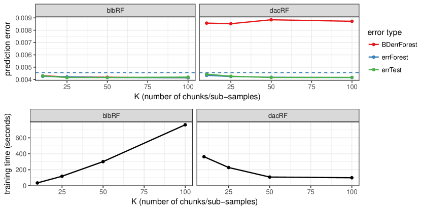
Figure 10: Evolution of prediction error (top) and computational time for training (bottom) versus $K$. $K$ is the number of chunks for dacRF (right) or the number of sub-samples for blbRF (left). The number of trees, $q$, is set to $10$.

Symmetrically, $K$ was then fixed to $10$ to illustrate the effect of the number of trees in each chunk/sub-samples. Results are provided in Figure 11. Again, blbRF is quite robust to the choice of $q$. On the contrary, for dacRF, the number of trees built in each chunk must be quite high to get an unbiased BDerrForest, at a cost of a substantially increased computational time. In other simulations for dacRF, $q$ was also set to $100$ and $K$ was increased but this did not give any improvement (not shown).

Figure 11: Evolution of the prediction error (top) and computational time for training (bottom) versus $q$. $q$ is the number of trees in each chunk for dacRF (right) or the number of trees in each sub-sample for blbRF (left). $K$ is set to $10$.

Due to these conclusions, the values $K=10$ and $q=50$ were chosen for blbRF and the values $K=10$, $q=100$ were chosen for dacRF in the rest of the simulations.

Second, the impact of the sampling fraction, $f=\frac{m}{n}$ was studied for sampRF and moonRF, with a number of trees set to $100$. More precisely, for sampRF, a subsample containing $m$ observations was randomly drawn for the entire dataset, with $f\in\{0.1,1,10\}$%. Results (see the right-hand side of Figure 12) show that BDerrForest is quite unbiased as soon as $f$ is larger than 1%. Furthermore, $f=10$% leads to some increase in computational time needed for training, even if this time is around $10$ times smaller than the one needed to train dacRF with $10$ chunks and $100$ trees.

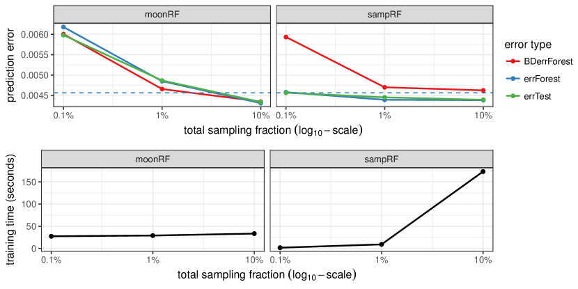
Figure 12: Evolution of the prediction error (top) and computational time for training (bottom) versus the sampling fraction ($\log_{10}$-scale) used in moonRF (left) and sampRF (right). The number of trees is set to $100$.

For moonRF, as the $100$ trees are built on samples with $m$ different observations each, the sampling fraction was varied in $\{10^{-5},10^{-4},10^{-3}\}$, in order to get a fraction of observations used by the entire forest (total sampling fraction, represented on the $x$-axes of the figure) comparable to the one used in sampRF. The left-hand part of Figure 12 shows that BDerrForest gives quite unbiased estimations of the prediction error. Moreover, the computational time for training remains low. The increase of the prediction error when $f=0.1$% is explained by the fact that subsamples contain only $150$ observations in this case. Based on these experiments, the total sampling fraction was set to 1% for both sampRF and moonRF in the rest of the simulations.

Several conclusions can be driven from these results. First, the computational time needed to train all these Big Data versions of RF is almost the same and quite reduced (about a few minutes) compared to the sequential RF. The fastest approach is to extract a very small subsample and the slowest is the dacRF approach with 10 chunks of 100 trees each (because the number of observations sent to each chunk is not much reduced compared to the original dataset). The results are not shown for the sake of simplicity but the performances are also quite stable: when a method was trained several times with the same parameters, the performances were almost always very close.

Regarding the errors, it has first to be noted that the prediction error (as assessed with errTest) is much better estimated by errForest than by the proxy of the OOB error provided by BDerrForest. In particular, BDerrForest tends to be biased for sampRF and moonRF approaches when the fraction of samples is very small and it tends to overestimate the prediction error (sometimes strongly) for dacRF.

Finally, many methods achieve a performance which is quite close to that of the standard RF algorithm: sampRF and moonRF approaches are quite close to the standard algorithm seqRF, even for very small subsamples (with at least 0.1% of the original observations, the difference between the two predictors is not very important). blbRF is also quite close to seqRF and remarkably stable to a change in its parameters $K$ and $q$. Finally, dacRF also gives an accurate predictor but its BDerrForest error estimation is close to the prediction error only when the number of trees in the forest is large enough: this is obtained at the price of a higher computational cost (about 10 times larger than for the other approaches).

4.3 More about subsampling biases and tree depth

In the previous section, simulations were conducted with representative subsamples and a maximum number of leaves equal to 500 for every tree in every forest. The present section pushes the analysis a bit further by specifically investigating the influence of these two features on the results. All simulations were performed with the same dataset and the same computing environment than in the previous section. Finally, the different parameters for the RF methods were fixed in light of the previous section: blbRF and dacRF were learned respectively with $K=10$ and $q=50$ and with $K=10$, $q=100$, whereas moonRF and sampRF were learned with total sampling fraction equal to $0.1$%.

As explained in Section 3.2, dacRF can be influenced by the lack of representativity of the data sent to the different chunks. In this section, we evaluate the influence of such cases in two different directions. We have considered the non representativity of observations in the different chunks/sub-samples, firstly according to $Y$ values using the unbalanced dataset and secondly, according to $X$ values using the x-biases dataset (see Section 4.1 for a description of these two datasets). For dacRF, this simulation corresponds to the case where the subforests built from the different chunks are very heterogeneous. This issue has been discussed in Section 3.2.3 and we will show that it indeed has a strong impact in practice.

Results associated to the unbalanced case are presented in Figure 13. In this case, data are organized so that, for dacRF, half of the chunks have a proportion $p\in\{0.01,0.1\}$ of observations from the first class ($Y=1$), and the other half have the same proportion of observations from the second class ($Y=-1$). For blbRF and moonRF, half of the sub-samples were drawn in order to get a proportion $p$ of observation from the first class and the other half the same proportion of observations from the second class. Finally, as there is only one subsample to draw for sampRF, it has been obtained with a proportion $p$ of observations of the first class. Hence, the results associated to sampRF are not fully comparable to the other two.

Figure 13: Prediction error behavior for 4 RF methods for unbalanced data. Unbalanced proportion $p$ is set to 0.01 (left) or to 0.1 (right).

The first fact worth noting in these results is again that errOOB and errTest are always very close, whereas BDerrForest is more and more biased as $p$ decreases. For $p=0.1$, BDerrForest bias is rather stable for all methods, except for sampRF (which is explained by the fact that only one subsample is chosen and thus 90% of the observations are coming from the second class). When $p=0.01$ (which corresponds to a quite extreme situation), we can see that dacRF is the most affected method, in terms of BDerrForest (BDerrForest strongly underestimates the prediction error) but also in terms of errOOB and errTest because these two quantities increase a lot.

Interestingly, moonRF is quite robust to this situation, whereas blbRF has a BDerrForest which strongly overestimates the prediction error. The difference of behavior between these two last methods might from the fact that, in our setting, 100 sub-samples are drawn for moonRF but only 10 for blbRF.

A similar conclusion is obtained for biases towards $X$ values: simulations have been performed for dacRF with x-biases obtained by partitionning the data into 2 parts (as illustrated on the right-hand side of Figure 8), leading to 7/10 of the $K=10$ chunks of data to contain only observations from submodel 1 and the other 3/10 chunks contaning only observations from submodel 2. Results are given in Figure 14.

Figure 14: Prediction errors for x-biases with dacRF ($K=10$ and $q=100$).

This result shows that the performance of the forest is strongly deteriorated when subforests are based on observations coming from different distributions $X|Y$: in this case, the test misclassification rate is multiplied by a factor of more than 50. Moreover, BDerrForest appears to be a very bad estimation of the prediction error of the forest.

Finally, the issue of tree depth is investigated more closely. As mentioned above, the maximum number of leaves was set to 500 in order to get comparable tree complexities. However homogeneity (in terms of classes) of leaves differs when a tree is built on the entire dataset or on a fraction of it. To illustrate this, the mean Gini index (over all leaves of a tree and over 100 trees) was computed (it is defined by $2\hat{p}(1-\hat{p})$, with $\hat{p}$ the proportion of observations of class 1 in a leaf). Results are reported in Table 6.

Sampling Comp. Max. tree Pruned tree mean Gini fraction time size size 100% 5 hours 60683 3789 0.233 10% 13 min 6999 966 0.183 1% 23 sec 906 187 0.073 0.1% 0.01 sec 35 10 0.000

Table 6: Number of leaves and leaves heterogeneity of trees built on various fractions of data. Second column indicates computational time needed to built one tree, while number of leaves of the maximal tree and the optimal pruned tree are given in third and fourth column respectively. The last column the mean Gini index over all leaves of a tree and over 100 trees.

For sampling fractions equal to 0.1% or 1%, tree leaves are pure (i.e., contain observations from only one class). But for sampling fractions equal to 100% and 10%, the heterogeneity of the leaves is more important. The effect of trees depth on RF performance was thus investigated. Recall that in RF all trees are typically grown to maximal trees (splits are performed until each leaf is pure) and that in CART an optimal tree is obtained by pruning the maximal tree. Table 6 contains the number of leaves of the maximal tree and the optimal CART tree associated to each sampling fraction. Trees with 500 leaves are very far from maximal trees in most cases and even far from optimal CART tree for sampling fractions equal to 100% and 10%.

Finally, performance of 3 RF methods using maximal trees instead of 500 leaves trees were obtained. The results are illustrated in Figure 15.

Figure 15: Prediction error (mesured by errTest) behavior for 3 RF methods when using maximal trees or a maximum number of leaves of 500.

Computational times are comparable to those shown in Figures 11 and 12, while the misclassification rates are slightly better. The remaining heterogeneity, when developing trees with 500 leaves, does not affect much the performance in that case. Hence, while pruning all trees would lead to a prohibitive computational time, a constraint on tree size may well be adapted to the Big Data case. This point needs a more in-depth analysis and is left for further research.

4.4 Online random forest

This section is dedicated to simulations with online RF. The simulations were performed with the method described in [20] which is available at https://github.com/david-matheson/rftk (onRF). The method is implemented in python. Thus computational time cannot be directly compared to the computational described in the two previous sections (because of the programming language side effect). Similarly, the input hyperparameters of randomForest function in the R package randomForest are not exactly the same than the ones proposed in onRF: for instance, in the R package, the complexity of each tree is controlled by setting the maximum number of leaves in a tree whereas in onRF, it is controlled by setting the maximum depth of the trees. Additionally, the two tools are very differently documented: every function and option in the R package are described in details in the documentation whereas RFTK is not provided with a documentation. However, the meaning of the different options and outputs of the library can be guessed from their names in most cases.

When relevant, we discuss the comparison between the standard approaches tested in the two previous sections and the online RF tested in the current version but the reader must be aware that some of the differences might come directly from the method itself (standard or online), whereas others come from the implementation and programming languages and that it is impossible to distinguish between the two in most cases.

The simulations in this section were performed on the datasets described in Section 4.1. The training dataset (randomly ordered) took approximately 9 minutes to be loaded with the function loadtxt of the python library numpy, which is about 9 times larger than the time needed by the R package readr to perform the same task. In the sequel, results about this dataset will be referred as standard. Moreover, simulations were also performed to study the effect of sampling (subsamples drawn at random with a sampling fraction in $\{0.01,0.1,1,10\}$%) or of biased order of arrival of the observations (with the datasets unbalanced, with $p=0.01$, and x-biases with 15 parts). For x-biases the number of parts was chosen differently than in the Section 4.2 (for dacRF) because only 2 parts would have led to a quite extreme situation for onRF, in which all data coming from submodel 1 are presented first, before all data coming from submodel 2 are presented. We have thus chosen a more moderate situations in which data from the two submodels are presented by blocks, alternating submodel 1 and submodel 2 blocks. Note that both simulation settings are similar, since dacRF processes the different (biased in $X$) blocks in parallel.

The forests were trained with a number of trees equal to 50 or 100 (for approximately 500 trees, the RAM capacity of the server was overloaded) and with a control of the complexity of the trees by their maximum depth which was varied in $\{5,10,15,50\}$. RFTK does not provide the online approximation of OOB error so the accuracy was assessed by the computation of the prediction error on the same test dataset used in the previous two sections.

Figure 16 displays the misclassification rate of onRF on the test dataset versus the type of bias in the order of arrival of data (no bias, unbalanced or x-biases) and versus the number of trees in the forest. The results are provided for forests in which the maximum depth of the trees was limited to 15 (which almost always correspond to fully developed trees).

Figure 16: onRF: Prediction error for the test dataset.

The result shows that, contrary to the dacRF case, x-biases almost do not affect the accuracy of the results, even if the classifier always has a better accuracy when data are presented in random order. On the contrary, unbalanced has a strong negative impact on accuracy of the classifier. Finally, for the best case scenario (standard), the accuracy of onRF is not much affected by the number of trees in the forest but the accuracy tends to get even worse when increasing the number of trees in the worst case scenario (unbalanced). In comparison with the strategies described in Section 4.2, onRF has comparable test error rates (between $(4-4.3)\times 10^{-3}$) for forests with 100 trees).

Additionally, Figure 17 displays the evolution of the computational time versus the type of bias in the order of arrival of data and the number of trees in the forest. The results are provided for forests in which the maximum depth of the trees was limited to 15.

Figure 17: Training time (seconds) of onRF.

As expected, computational time increases with the number of trees in the forest (and the increase is larger than the increase in the number of trees). Surprisingly, the computational time of the worse case scenario (unbalanced bias) is the smallest. A possible explanation is the fact that trees are presented successively a large number of observations with the same value of the target variable ($Y$): the terminal nodes are thus maybe more easily pure during the training process in this scenario.

Computational times are hard to compare with the ones obtained in Section 4.2. However, computational times are of order 30 minutes at most for dacRF, and 1-2 minutes for blbRF and moonRF, whereas onRF takes approximately 10 hours for 50 trees and 30 hours for 100 trees, which is even larger than training the forest sequentially with randomForest (7 hours).

Figure 18 displays the evolution of the misclassification rate and of the computational time versus the sampling fraction when a random subsample of the dataset is used for the training (the number of trees in the forest is equal to 100 and the maximum depth set to 15). The computational time needed to train the model is more than linear but the prediction accuracy also decreases in a more than linear way with the sampling fraction. The loss in accuracy is slightly worse than what was obtained in Section 4.2 for sampRF, showing than onRF might need a

Figure 18: Prediction error (left) and training time (right) versus sampling fraction for onRF. $x$-axis is $\log_{10}$-scaled.

Finally, Figure 19 displays the evolution of the test misclassification rate, of the computational time and of the average number of leaves in the trees versus the value of the maximum depth for forests with 100 trees. As expected, the computational time is in direct relation with the complexity of the forest (number of trees and maximum depth) but tends to remain almost stable for trees with maximum depth larger than 15. The same behavior is observed for the misclassification rate in standard and x-biases which reach their minimum for forests with a maximum depth set to 15. Finally, the number of leaves for unbalanced is much smaller, which also explains why the computational time needed to train the forest in this case is smaller. For this type of bias, the misclassification rates increases with the maximum depth for forest with maximum depths larger than 10: as for the number of trees, the complexity of the model seem to have a negative impact on this kind of bias.

Figure 19: Top: Average depth of trees in the forest. Bottom: Average number of leaves of trees in the forest. The black horizontal line corresponds to the maximum number of leaves used in experiments of Sections 4.2 and 4.3.

4.5 Airline dataset

In the present section, similar experiments are performed with a real world dataset related to flight delays. The data were first processed in [6] to illustrate the use of the R packages for Big Data computing bigmemory and foreach [38]. In [6], the data were mainly used for description purpose (e.g., quantile calculation), whereas we will be using it for prediction. More precisely, five variables based on the original variables included in the data set were used to predict if the flight was likely to arrive on time or with a delay larger than 15 minutes (flights with a delay smaller than 15 minutes were considered on time). The predictors were: the moment of the flight (two levels: night/daytime), the moment of the week (two levels: weekday/week-end), the departure time (in minutes, numeric) and distance (numeric). The dataset used to make the simulations contained 120,748,239 observations (observations with missing values were filtered out) and had a size equal to 3.2 GB (compared to the 12.3 GB of the original data with approximately the same number of observations). Loading the dataset and processing it to compute and extract the predictors and the target variables took approximately 30 minutes. Another feature of the dataset is that it is unbalanced: most of the flight are on time (only 19.3% of the flights are late).

The same method than the one described in Section 4.2 were compared:

• a standard RF, seqRF, was computed sequentially. It contained 100 trees. The RF took 16 hours to be obtained and its OOB error was equal to 18.32%;

• sampRF was trained with a subsample of the total data (1% of all the observations were sampled at random without replacement). These RF were trained in parallel with 15 cores, each core building 7 trees from bootstrap samples coming from the common subsample (the final RF hence contained 105 trees);

• a blbRF was also trained using $K=15$ subsamples, each containing about 454,272 observations (about 0.4% of the size of the total data set). 15 sub-forests were trained in parallel with 7 trees each (the final forest hence contained 105 trees);

• Finally dacRF was also obtained with $K=15$ chunks and $q=7$ trees in each sub-forest grown in the different (the final RF contained from to 1000 trees).

The number of trees, $q$, built in each chunk for dacRF is smaller than what seemed a good choice in Section 4.2, but for this example, increasing the number of trees did not lead to better accuracy (even if it increased a lot the computational time).

In all methods, the maximum number of terminal leafs in the trees was set to 500 and all RF were trained in parallel on 15 cores, except for the sequential approach. Results are given in Figure 20 in which the notations are the same as in Section 4.2.

Figure 20: Performance (computational time and misclassification rates) obtained by three different RF methods for Big Data on Airline data.

The results show that there is almost no difference in terms of performance accuracy between using all data and using only a small proportion (about 0.01%) of them. In terms of compromise between computational time and accuracy, using a small subsample is clearly the best strategy, provided that the user is able to obtain a representative subsample at a low computational cost. Also, contrary to what happened in the example described in Section 4.3, BDerrForest is always a good approximation of errForest. An explanation of this result might be that for Airline dataset, prediction accuracy is quite poor and this might be due to explanatory variables that are not informative enough. Hence differences between BDerrForest and errForest may be hidden by the fact that the two estimations of the prediction error are quite high.

In addition, the impact of the representativity, with respect to the target variable, of the samples on which the RF were trained was assessed: instead of using a representative (hence unbalanced) sample from the total dataset, a balanced subsample (for 50% of delayed flights and 50% of on time flights) was obtained and used as the input data to train the random forest. Its size was equal to 10% of the total dataset size. This approach obtained an errForest equal to 33.34% (and BDerrForest was equal to 39.15%), which is strongly deteriorated compared to the previous misclassification rates. In this example, the representativity of the observations contained in the subsample strongly impacts the estimated model. The model with balanced data has a better ability to detect late flights and favors the sensitivity over the specificity.

5 Conclusion and discussion

This final section provide a short conclusion and opens two perspectives. The first one proposes to consider re-weighting random forests as an alternative for tackling the lack of representativeness for BD-RF and the second one focuses on alternative online RF schemes as well RF for data streams.

5.1 Conclusions

This paper aims at extending standard Random Forests in order to process Big Data. Indeed RF is an interesting example among the widely used statistical methods in machine learning since it already offers several ways to deal with massive data in offline or online contexts. Focusing on classification problems, we reviewed some of the available proposals about RF in parallel environments and online RF. We formulated various remarks for RF in the Big Data context, including approximations of out-of-bag type errors. We experimented on two massive datasets (15 and 120 millions of observations), a simulated one and real world data, five variants involving subsampling, adaptations of bootstrap to Big Data, a divide-and-conquer approach and online updates.

Among the variants of RF that we tested, the fastest were sampRF with a small sampling fraction and blbRF. On the contrary, onRF was not found computationally efficient, even compared to the standard method seqRF, in which all data are processed as a whole and trees are built sequentially. On a performance point of view, all methods provide satisfactory results but parameters (size of the subsamples, number of chunks…) must be designed with care so as to obtain a low prediction error. However, since the estimation of OOB error that can be simply designed from the different variants was found a bad estimate of the prediction error in many cases, it is also advised to rather calculate an error on an independent smaller test subsample. When the amount of data is that big, computing such a test error is easy and can be performed at low computational cost.

Finally, one of the most crucial point stressed in the simulations is that the lack of representativeness of subsamples can result in drastic deterioration of the performances of Big Data variants of RF, especially of dacRF. However, designing a subsample representative enough of the whole dataset can be an issue per se in the Big Data context, but this problem is out of the scope of the present article.

5.2 Re-weighting schemes

As an alternative, some re-weighting schemes could be used to address the issue of the lack of representativeness for BD-RF. Let us sketch some possibilities.

Following a notation from Breiman [21], RF lead to better results when there is a higher diversity among the trees of the forest. So recently, some extensions of RF have been defined for improving an initial RF. In [39], Fawagreh et al. use an unsupervised learning technique (Local Outlier Factor, LOF) to identify diverse trees in the RF and then, they perform ensemble pruning by selecting trees with the highest LOF scores to produce an extension of RF termed LOFB-DRF, much smaller in size than RF and performing better. This scheme can be extended by using other diversity measures, see [40] presenting a theoretical analysis on six existing diversity measures.

Another possible variant would be to consider the whole forest as an ensemble of forests and to adapt the majority vote scheme with weights that address, e.g., the issue of the sampling bias. Recently in [41], Winham et al. propose to introduce a weighted RF approach to improve predictive performance: the weighting scheme is based on the individual performance of the trees and could be adapted to the dacRF framework.

Along the same ideas it would be, at least for an exploratory stage, possible to adapt a simple idea coming from the variants of AdaBoost [42] for classification boosting algorithms. Recall that the basic idea of boosting is, as for the RF case, to generate many different base predictors obtained by perturbing the training set and to combine them. Each predictor is designed sequentially highlighting the observations poorly predicted. This is a crucial difference with RF scheme for which the different training samples are obtained by independent bootstraps. But the aggregation part of the algorithm is interesting here: instead of taking the majority vote of the trees predictions as in the RF context, a weighted combination of trees is considered. The unnormalized weight of the tree $t$ is simply $\alpha_{t}=1/2\ln(\epsilon_{t}/(1-\epsilon_{t}))$ where $\epsilon_{t}$ is the misclassification error computed on the whole training sample $L$. This could be adapted by considering weighted forests using weights of such form, evaluated on a same (small) subset of observations supposed to be representative of the whole dataset.

5.3 Online data and Data Streams

The discussion sketched about online RF can be extended. Indeed the use of ERT variant of RF instead of Breiman’s RF allows to reduce the computational cost. It would be of interest to use this RF variant in dacRF, or even more randomized ones (like [43] PERT, Perfect Random Tree Ensembles, or [44, 45] PRF, Purely Random Forests). The idea of those latter variants is to not choose the variable involved in a split and the associated threshold from the data but to randomly choose them according to different schemes. Finally, onRF could be a way to use only a portion of the data set until the forest is accurate enough. Moreover, one valuable characteristic of onRF is that it could address both the issue of Volume and Velocity.

In the framework of online RF, only sequential inputs are considered. But more widely in the Big Data context, data streams are of interest. They allows to consider not only sequential inputs, but also entail unbounded data that should be processed in limited (given their unboundedness) memory and in an online fashion to obtain real-time answers to application queries (for an accurate and formal one, see [46]). Moreover, data streams can be processed in observation- or time-based windows or even batches which collect a number of recent observations (see for instance [47]). It could be interesting to fully adapt online RF to the data stream context (see for example [48] and [49]) and obtain similar theoretical results.

Additional Files

Additional file 1 — R and python scripts used for the simulation

R scripts used in the simulation sections are available at https://github.com/tuxette/bigdatarf.

References

- [1] J. Fan, F. Han, H. Liu, Challenges of big data analysis, National Science Review 1 (2) (2014) 293–314. doi:10.1093/nsr/nwt032.
- [2] R. Hoerl, R. Snee, R. De Veaux, Applying statistical thinking to ‘Big Data’ problems, Wiley Interdisciplinary Reviews: Computational Statistics 6 (4) (2014) 222–232. doi:10.1002/wics.1306.
- [3] M. Jordan, On statistics, computation and scalability, Bernoulli 19 (4) (2013) 1378–1390. doi:10.3150/12-BEJSP17.
-
[4]
P. Besse, A. Garivier, J. Loubes, Big
data - Retour vers le futur 3. De statisticien à data scientist, arXiv
preprint arXiv:1403.3758 (2014).
URL http://arxiv.org/abs/1403.3758 - [5] A. Thusoo, Z. Shao, S. Anthony, D. Borthakur, N. Jain, J. Sen Sarma, R. Murthy, H. Liu, Data warehousing and analytics infrastructure at facebook, in: Proceedings of the ACM SIGMOD International Conference on Management of Data (SIGMOD 2010), 2010, pp. 1013–1020.
-
[6]
M. Kane, J. Emerson, S. Weston,
Scalable strategies for computing
with massive data, Journal of Statistical Software 55 (14).
URL http://www.jstatsoft.org/v55/i14 -
[7]
R Core Team, R: A Language and Environment
for Statistical Computing, R Foundation for Statistical Computing, Vienna,
Austria (2016).
URL http://www.R-project.org -
[8]
P. Besse, N. Villa-Vialaneix, Statistique
et big data analytics. Volumétrie, l’attaque des clones, arXiv preprint
arXiv:1405.6676 (2014).
URL http://arxiv.org/abs/1405.6676 - [9] C. Wang, M. Chen, E. Schifano, J. Wu, J. Yan, A survey of statistical methods and computing for big data, arXiv preprint arXiv:1502.07989 (2015).
- [10] M. Bǎdoiu, S. Har-Peled, P. Indyk, Approximate clustering via core-sets, in: J. Reif (Ed.), Proceedings of the 34th annual ACM Symposium on Theory of Computing, no. 250-257, ACM New York, NY, USA, Montreal, QC, Canada, 2002. doi:10.1145/509907.509947.
- [11] D. Yan, L. Huang, M. Jordan, Fast approximate spectral clustering, in: J. Elder, F. Soulié-Fogelman, P. Flach, M. Zaki (Eds.), Proceedings of the 15th ACM SIGKDD international Conference on Knowledge Discovery and Data Mining, ACM New York, NY, USA, 2009, pp. 907–916. doi:10.1145/1557019.1557118.
- [12] A. Kleiner, A. Talwalkar, P. Sarkar, M. Jordan, A scalable bootstrap for massive data, Journal of the Royal Statistical Society: Series B (Statistical Methodology) 76 (4) (2014) 795–816.
- [13] N. Laptev, K. Zeng, C. Zaniolo, Early accurate results for advanced analytics on MapReduce, in: Proceedings of the 28th International Conference on Very Large Data Bases, Vol. 5 of Proceedings of the VLDB Endowment, Istanbul, Turkey, 2012.
- [14] X. Meng, Scalable simple random sampling and stratified sampling, in: Proceedings of the 30th International Conference on Machine Learning (ICML 2013), Vol. 28 of JMLR: W&CP, Georgia, USA, 2013.
- [15] C. Chu, S. Kim, Y. Lin, Y. Yu, G. Bradski, A. Ng, K. Olukotun, Map-Reduce for machine learning on multicore, in: J. Lafferty, C. Williams, J. Shawe-Taylor, R. Zemel, A. Culotta (Eds.), Advances in Neural Information Processing Systems (NIPS 2010), Vol. 23, Hyatt Regency, Vancouver, Canada, 2010, pp. 281–288.
- [16] X. Chen, M. Xie, A split-and-conquer approach for analysis of extraordinarily large data, Statistica Sinica 24 (2014) 1655–1684.
- [17] S. del Rio, V. López, J. Benítez, F. Herrera, On the use of MapReduce for imbalanced big data using random forest, Information Sciences 285 (2014) 112–137. doi:10.1016/j.ins.2014.03.043.
- [18] V. Chandrasekaran, M. Jordan, Computational and statistical tradeoffs via convex relaxation, Proceedings of the National Academy of Sciences USA 13 (2013) E1181–E1190.
- [19] A. Saffari, C. Leistner, J. Santner, M. Godec, H. Bischof, On-line random forests, in: Proceedings of IEEE 12th International Conference on Computer Vision Workshops (ICCV Workshops), IEEE, 2009, pp. 1393–1400.
- [20] M. Denil, D. Matheson, N. de Freitas, Consistency of online random forests, in: Proceedings of the 30th International Conference on Machine Learning (ICML 2013), 2013, pp. 1256–1264.
-
[21]
L. Breiman,