Abstract

In the context of minimal supersymmetric standard model (MSSM), we discuss the possibility of the lightest Higgs boson with mass $M_{h}=98$ GeV to be consistent with the $2.3\sigma$ excess observed at the LEP in the decay mode $e^{+}e^{-}\to Zh$, with $h\to b{\bar{b}}$. In the same region of the MSSM parameter space, the heavier Higgs boson $(H)$ with mass $M_{H}\sim 125$ GeV is required to be consistent with the latest data on Higgs coupling measurements at the end of 7 + 8 TeV LHC run with $25{\rm fb}^{-1}$ of data. While scanning the MSSM parameter space, we impose constraints coming from flavour physics, relic density of the cold dark matter as well as direct dark matter searches. We study the possibility of observing this light Higgs boson in vector boson fusion process and associated production with $W/Z$ boson at the high luminosity $(3000~{}{\rm fb}^{-1})$ run of the 14 TeV LHC. Our analysis shows that this scenario can hardly be ruled out even at the high luminosity run of the LHC. However, the precise measurement of the Higgs signal strength ratios can play a major role to distinguish this scenario from the canonical MSSM one.

 

 

1 Introduction

The LHC has recently started its second phase of run. The discovery of a new scalar particle of mass $\sim$ 125 GeV has been confirmed [1]. The properties of this newly discovered resonance seem to be in close agreement with that of the Standard Model (SM) Higgs boson of the same mass [2]. The production modes for the Higgs boson at the LHC are those via the gluon-gluon fusion, the vector boson ($W^{\pm},Z$) fusion and the associated production with a vector boson ($W^{\pm},Z$) or top quarks whereas its most effective decay modes are into 4 leptons ($e$ and $\mu$) , $W^{+}W^{*-}$, and $\gamma\gamma$ channels. One of the main goals of the current LHC run with increased centre of mass energy and higher luminosity is to find out whether the discovered particle is the Standard Model Higgs boson or a part of an extended Higgs sector containing several other physical scalars.

The Higgs sector of the Minimal Supersymmetric Standard Model (MSSM) [3, 4, 5, 6] has a far richer spectrum than that of the SM. The model has two CP-even neutral scalars (the lighter and the heavier ones $h$ and $H$ respectively), one CP-odd neutral scalar ($A$) and two charged scalars ($H^{\pm}$). At the tree level, only two input parameters other than the Z-boson mass ($M_{Z}$) are required to specify the Higgs sector of the MSSM. These inputs are $(i)$ the mass of the pseudoscalar Higgs boson ($M_{A}$) and $(ii)$ the ratio of vaccum expectation values (vevs) of the two Higgs doublets of the MSSM ($\tan\beta$). Dependence on other input parameters are induced once the radiative corrections to the Higgs mass are taken into account. We note that the couplings of $H$ to the gauge bosons such as $HZZ$, $HW^{+}W^{-}$ are proportional to $\cos(\beta-\alpha)$ where $\alpha$ is the Higgs mixing angle[6]. On the other hand, couplings like $hZZ$, $hW^{+}W^{-}$ are proportional to $\sin(\beta-\alpha)$.

In the well-known decoupling limit of the MSSM[6] characterized by the mass hierarchy $M_{H}\simeq M_{A}\simeq M_{H^{\pm}}\gg M_{Z},M_{h}$, all the Higgs bosons become much heavier than the lightest one ($h$) making the latter to have SM-like mass as well as couplings. In this limit one has $\cos(\beta-\alpha)\rightarrow 0$ indicating negligibly small values for the aforesaid couplings of the heavier Higgs bosons. Thus, it seems natural to consider the Higgs particle observed at the LHC as the lightest CP-even Higgs of the MSSM in the decoupling limit. However, the other possibility of having a non-decoupling regime of the MSSM where the observed boson at 125 GeV is interpreted as the heavier CP-even Higgs scalar $H$ can be consistent with the non-decoupling regime of the MSSM Higgs bosons where $M_{h}\sim M_{H}\sim M_{A}\sim M_{Z}$[6]. In this case, all the MSSM Higgses would be light with the lightest one lying somewhat below 125 GeV. The above non-decoupling scenario may get its motivation from an old result by the LEP collaboration which corresponds to an excess of Higgs-like events around a mass of 98 GeV [7, 8]. The excess was found in the channel $e^{+}e^{-}\rightarrow Zh$ with $h$ decaying into $b\bar{b}$. In a combined analysis of the four LEP working groups this excess reached a significance of 2.3$\sigma$. The above phenomena can not be explained within the SM since the SM Higgs boson would give rise to a larger production cross-section. In our previous analysis of Ref.[9] we explored the possibility of interpreting the 2.3$\sigma$ excess events in the MSSM with the name ‘Inclusive LEP-LHC Higgs (ILLH) scenario’ where $h$ and $H$ are required to correspond to the LEP excess near 98 GeV and the observed resonance at $\sim$ 125 GeV at the LHC respectively. There have been several studies in this direction and a partial list may be seen in Ref.[10, 11, 12, 13, 14, 15, 16, 17, 18, 19, 20, 21, 22, 23, 24]. In spite of the fact that the above MSSM scenario is believed to be cornered in recent times [25], we believe that it is important to review the current status of the scenario in relation to the latest LHC data via focussing our attention in relevant zones of appropriate parameters of MSSM in a model independent way.

We must note that if this scenario is indeed realized then $(i)$ the value of $\sin^{2}(\beta-\alpha)$ must be very small in order to explain the small $ZZh$ coupling at LEP and $(ii)$ the couplings of $H$ must be similar to that of the SM Higgs in order to be compatible with the 125 GeV resonance observed at the LHC. The parameter region which satisfies these two requirements must also pass through other direct constraints coming from the LHC, the most important ones are given as below.

• Exclusion limits in the channel $H/A\rightarrow\tau^{+}\tau^{-}$ : Both the ATLAS and CMS collaborations have searched for a neutral Higgs-like boson $\Phi$ in the decay channel $\tau^{+}\tau^{-}$ for certain benchmark scenarios [26, 27]. However, in order to perform a model-independent analysis one must consider the bounds on $\sigma\times{\rm BR}(\Phi\to\tau^{+}\tau^{-})$ as a function of $m_{\Phi}$, where $\sigma$ denotes the production cross-section for the non-minimal Higgs boson $\Phi$ decaying into the di-tau channel. Two different production modes for $\Phi$ are considered namely, the gluon-gluon fusion and the associated production with b-quark.

• Searches for $H^{\pm}$ : The ATLAS and CMS searches for $H^{\pm}$ are performed in $t\bar{t}$ events with subsequent decays $t\rightarrow bH^{\pm}$ and $H^{\pm}\rightarrow\tau\nu$ [28, 29]. Model-independent upper bounds are obtained for ${\rm BR}(t\rightarrow bH^{\pm})\times{\rm BR}(H^{\pm}\rightarrow\tau\nu)$. These searches exclude $\tan\beta$ up to 6 for 90 GeV $<M_{H^{\pm}}<$ 150 GeV.

These two searches together restrict $\tan\beta$ to have a very narrow range. Moreover, the constraints from heavy flavor physics also become very important in this region of parameter space. In particular, experimental limits on ${{\rm BR}(b\to s\gamma)}$ and ${{\rm BR}(B_{s}\to\mu^{+}\mu^{-})}$ are able to play very crucial roles to constrain the MSSM parameter space under question.

In Ref.[9] we imposed all of the above bounds on the MSSM parameter space to probe whether it could accommodate the ILLH scenario. However, for the Higgs signal strength constraints we used a conservative lower bound on ${\mu}^{\gamma\gamma}_{gg}$ (see Eq.3) taken as ${\mu}^{\gamma\gamma}_{gg}>0.5$. Afterwards, the bounds from the ATLAS and CMS collaborations for the pseudoscalar and charged Higgs search channels have become more stringent. On the other hand, the Higgs signal strength results have become more precise in recent times. Thus it seems very reasonable to reanalyze the 98-125 GeV Higgs scenario in the light of the updated collider constraints and to check whether there is any room left in the MSSM framework to accommodate a 98 GeV Higgs boson.

In this work we perform a detailed scan over the MSSM parameter space to find out the region allowed by all the relevant collider constraints mentioned above. We also demand that the MSSM parameter space must satisfy the PLANCK limit on dark matter relic density. Keeping these issues in mind we explore the possibility of observing the signals of the ILLH scenario in the high-luminosity run of the LHC. The plan of this paper is as follows.

In Sec. 2 we discuss the major constraints imposed on the MSSM parameter space of our interest and the parameter ranges we choose to perform the scanning procedure. The impact of the constraints on the MSSM parameter space as well as the main features of the allowed zone are studied in Sec. 3. In Sec. 4 we analyze the prospects of the ILLH scenario in the high luminosity run of the LHC. Finally, we conclude in Sec. 5.

2 Relevant constraints and parameter space scanning

In this section we enumerate the essential constraints and the scanning details of the MSSM parameter space considered in this analysis.

2.1 The basic constraints for the ILLH scenario

The ILLH scenario requires that the lightest CP-even Higgs boson should have a mass around 98 GeV, while the one observed at the LHC at 125 GeV to be the heavier CP-even Higgs boson. Thus, we consider the following ranges for $M_{h}$ and $M_{H}$.

$$95~{}{\rm GeV}<M_{h}<101~{}{\rm GeV},$$

$$122~{}{\rm GeV}<M_{H}<128~{}{\rm GeV}.$$ (1)

An uncertainty of 3 GeV in the Higgs boson mass is assumed which may come from the top mass uncertainty, uncertainties in the renormalization scheme and higher order loop corrections [30]. The value of $\sin^{2}(\beta-\alpha)$ must lie within the following range in order to satisfy the LEP limit.

$$0.1<\sin^{2}(\beta-\alpha)<0.25.$$ (2)

2.2 Constraints from the LHC

The different production mechanisms of the Standard Model Higgs boson at the LHC are the gluon-gluon fusion (ggF), vector boson fusion (VBF) and associated production with gauge bosons ($VH$, $V=W^{\pm},Z$) or with a pair of top quarks ($t\bar{t}H$). Among its various possible decay modes, the decay into a pair of bottom quarks is the most dominant one. Other sub-dominant decay modes include final states involving a pair of SM gauge bosons ($VV^{*}$), $\tau^{+}\tau^{-}$ and $\gamma\gamma$ etc. The di-photon final states refer to loop-induced phenomena involving $W$-boson and heavy fermion loops. Both the ATLAS and CMS collaborations have analyzed various production and decay modes of the Higgs boson observed at 125 GeV and put bounds on the various couplings of the SM Higgs. The signal strength parameter $\mu$ is defined as the ratio between the measured Higgs boson rate and its SM expectation as follows:

$${\mu}^{f}_{i}=\frac{\sigma_{i}\times{\rm BR}^{f}}{{(\sigma_{i})}_{\rm SM}\times{({\rm BR}^{f})}_{\rm SM}}.$$ (3)

Here, $\sigma_{i}$ represents the production cross-section for a given new physics model with $i$= ggF, VBF, VH and $t\bar{t}H$ processes for a generic Higgs boson $H$ with $f=\gamma\gamma$, $ZZ^{*}$, $WW^{*}$, $b\bar{b}$, $\tau^{+}\tau^{-}$ being the decay modes of the Higgs boson. The subscript “SM” represents the respective SM expectations. In Table 1, we display the most updated combined results on various Higgs signal strengths by the ATLAS and CMS collaborations [31]. The subscript ‘F’ denotes the combined data for the ggF and $t\bar{t}H$ process, while ‘V’ signifies the combined VBF and VH processes. Even though the Higgs production through the “fusion” (F) mode includes both the ggF and $t\bar{t}H$ processes, here we consider the ggF process only since $\frac{\sigma_{t\bar{t}H}}{\sigma_{ggF}}\sim$ 2% as estimated by the combined ATLAS & CMS data and also uncertainties in Higgs signal strength measurements associated to the $t\bar{t}H$ process being relatively large.

Channel	Combined ATLAS + CMS signal strength
${\mu}^{\gamma\gamma}_{F}$	$1.19^{+0.28}_{-0.25}$
${\mu}^{\rm WW}_{F}$	$1.0^{+0.23}_{-0.20}$
${\mu}^{\rm ZZ}_{F}$	$1.44^{+0.38}_{-0.34}$
${\mu}^{\rm bb}_{F}$	$1.09^{+0.93}_{-0.89}$
${\mu}^{\tau\tau}_{F}$	$1.10^{+0.61}_{-0.58}$
${\mu}^{\gamma\gamma}_{V}$	$1.05^{+0.44}_{-0.41}$
${\mu}^{\rm WW}_{V}$	$1.38^{+0.41}_{-0.37}$
${\mu}^{\rm ZZ}_{V}$	$0.48^{+1.37}_{-0.91}$
${\mu}^{\rm bb}_{V}$	$0.65^{+0.30}_{-0.29}$
${\mu}^{\tau\tau}_{V}$	$1.12^{+0.37}_{-0.35}$

Table 1: Combined results of the Higgs coupling measurements by the ATLAS and CMS collaborations at the end of 7 + 8 TeV run of the LHC with approximately 25 ${\rm fb}^{-1}$ of data [31]

At the end of 8 TeV run of the LHC, the signal strength variables associated with the observed 125 GeV Higgs boson still allow significant deviations from the SM predictions. Keeping this in mind, here we consider 2$\sigma$ deviations from the central value of various signal strength variables obtained after combining the ATLAS and CMS data.

$$0.69<{\mu}^{\gamma\gamma}_{F}<1.75,\quad 0.6<{\mu}^{WW}_{F}<1.46,\quad 0.76<{\mu}^{ZZ}_{F}<2.2,$$

$$-0.69<{\mu}^{bb}_{F}<2.95,\quad-0.06<{\mu}^{\tau\tau}_{F}<2.32,\quad 0.23<{\mu}^{\gamma\gamma}_{V}<1.93,$$

$$0.64<{\mu}^{WW}_{V}<2.2,\quad-1.34<{\mu}^{ZZ}_{V}<3.22,\quad 0.07<{\mu}^{bb}_{V}<1.25,$$

$$0.42<{\mu}^{\tau\tau}_{V}<1.86.$$ (4)

Apart from the above, there are two experimental constraints that play crucial roles in the parameter space of our interest namely the limits from direct searches of the pseudo-scalar and charged Higgs bosons at the LHC. We note that from the direct searches of the pseudo-scalar Higgs boson both the ATLAS and CMS collaborations have eliminated the zone $90<M_{A}<250$ GeV for $\tan\beta\mathrel{\mathchoice{\vbox{\offinterlineskip\halign{$\m@th\displaystyle\hfil#\hfil$\cr>\crcr\sim\crcr} }}{\vbox{\offinterlineskip\halign{$\m@th\textstyle\hfil#\hfil$\cr>\crcr\sim\crcr} }}{\vbox{\offinterlineskip\halign{$\m@th\scriptstyle\hfil#\hfil$\cr>\crcr\sim\crcr} }}{\vbox{\offinterlineskip\halign{$\m@th\scriptscriptstyle\hfil#\hfil$\cr>\crcr\sim\crcr} }}}$ 5.5 [26, 27]. On the other hand, the ATLAS and CMS have also searched for light charged Higgs bosons using $t\bar{t}$ events via $t\rightarrow bH^{+}$ mode with $H^{+}\rightarrow\tau^{+}\nu_{\tau}$ [28, 29]. The ATLAS analysis indicates that the regions of parameter space with $\tan\beta$ between 2 to 6 with $90<m_{H^{+}}<150$ GeV is disallowed. We note that the ATLAS and CMS exclusion limits are available for a few benchmark scenarios with specific choices of the MSSM model parameters (e.g. the so-called $m_{h}^{max},m_{h}^{mod\pm}$ etc. scenarios[26, 27, 28, 29]). However, these scenarios seem to be rather over-simplified. On the other hand, there exist model-independent limits on the production cross-section times branching ratio i.e., $\sigma\times{\rm BR}(\Phi\to\tau^{+}\tau^{-})$, for a non-standard Higgs boson $\Phi$ when it is produced via gluon-gluon fusion and b-quark associated processes [26, 27]. We use these model-independent limits in the present work.

2.3 Constraints from flavor physics and cosmological abundance of dark matter

The light pseudo-scalar and charged Higgs bosons naturally make the flavor physics constraints very significant for the parameter space of our interest. We consider the two most stringent rare b-decay constraints, namely ${{\rm BR}(b\to s\gamma)}$ and ${{\rm BR}(B_{s}\to\mu^{+}\mu^{-})}$, and allow $2\sigma$ deviation from the central limit [32],

$$2.82\times 10^{-4}<{{\rm BR}(b\to s\gamma)}<4.04\times 10^{-4},$$ (5)

$$1.57\times 10^{-9}<{{\rm BR}(B_{s}\to\mu^{+}\mu^{-})}<4.63\times 10^{-9}.$$ (6)

Following the analysis of the PLANCK experiment[34] as in Ref.[9], we take the DM relic density limits as $0.112<\Omega h^{2}<0.128$. However, in this analysis we allow the possibility of having a multicomponent DM scenario. Hence, we consider only the upper limit of the relic density constraint as given below.

$$\Omega_{{\widetilde{\chi}}_{1}^{0}}h^{2}<0.128.$$ (7)

This allows for the possibility of an under-abundant DM scenario with relic density lying below the lower limit of the PLANCK data. We also check the consistency with the upper bounds on the DM direct detection cross-section from the LUX [35] experiment.

2.4 Exploring the relevant MSSM parameter space for the ILLH scenario

Considering the data from $A/H\rightarrow\tau^{+}\tau^{-}$ and $H^{+}\rightarrow\tau^{+}\nu_{\tau}$ search channels as constraints, we focus on the ILLH scenario for a small range of $\tan\beta$, namely $1<\tan\beta<6.5$. Note that, LEP data [8] disfavors the region with $\tan\beta<3$ for SM-like SUSY Higgs boson search with SUSY breaking scale $M_{SUSY}=1$ TeV. However, for a 98 GeV non-SM-like Higgs boson $h$, $\tan\beta$ can indeed be smaller than 3. Thus, in our analysis we probe the regions with smaller values of $\tan\beta$. On the other hand, choice of a model independent approach for Higgs mass motivates us for scanning up to $\tan\beta=6.5$, a value higher than the limit of the ATLAS and CMS data.

We choose the decoupling zone ($\sim$ 3 TeV) for the first two generations of squarks and sleptons, considering the fact that there is no effect on the Higgs spectra in phenomenological MSSM (pMSSM) of the above scalars[36].

The parameter range over which we perform random scan can be listed as follows.

$$1<\tan\beta<6.5,~{}0.12<M_{A}<0.3~{}{\rm TeV},~{}0.3~{}{\rm TeV}<\mu<12~{}{\rm TeV}$$

$$0.05~{}{\rm TeV}<M_{1},M_{2}<1.5~{}{\rm TeV},~{}0.5~{}{\rm TeV}<M_{3}<3~{}{\rm TeV},$$

$$-8~{}{\rm TeV}<A_{t},A_{b}<12~{}{\rm TeV},~{}A_{u}=A_{d}=A_{\tau}=A_{e}=0,$$

$$0.3~{}{\rm TeV}<M_{\tilde{q}_{3}}<5~{}{\rm TeV},~{}{\rm where},~{}{\tilde{q}_{3}}\equiv{\tilde{t}_{L}},{\tilde{t}_{R}},{\tilde{b}_{L}},{\tilde{b}_{R}}$$

$$M_{{\tilde{q}}_{i}}=3~{}{\rm TeV},{\rm for}~{}i=1,2~{}~{}{\rm and}~{}~{}M_{{\tilde{l}}_{i}}=3~{}{\rm TeV},{\rm for}~{}i=1,2,3.$$ (8)

The relevant SM parameters are chosen as, ${m_{b}}^{\overline{\rm MS}}(m_{b})=4.19$ GeV and $m_{t}^{\rm pole}=173.3\pm 2.8$ GeV (a larger error amount is considered following the argument of Ref.[37]) and the strong coupling constant $\alpha_{s}(M_{Z})=0.1172$. Stringency of satisfying Eq.1 to Eq.7 or primarily Eq.1 and Eq.2 requires a very dense parameter scan. In this work, the number of parameter points scanned is more than 80 million over the above ranges.

The publicly available code SuSpect (version 2.43) [38] is used for spectrum generation and micrOmegas (version 3.6.9.2) [39] is used for calculating the relic density and flavor observables while the branching ratios of the Higgs bosons are computed via HDECAY [40]. We calculate the Higgs production cross-section using SuShi [41]. The lower limits on the sparticle masses are imposed from the LEP and LHC data. We consider the lightest top and bottom squark masses are greater than 500 GeV, while the gluinos are assumed to be heavier than 1.4 TeV [42]. We also impose the LEP limit on the lightest chargino mass to be 100 GeV [42]. The charge color breaking (CCB) constraints are already imposed by SuSpect while scanning the parameter space.

3 Result

In Fig. 1, we display the allowed parameter space in the $M_{A}-\tan\beta$ and $M_{H^{\pm}}-\tan\beta$ planes, where the red circles represent the points which satisfy all the constraints (Eqs. 1-6) except Eq. 7, while blue crossed points satisfy Eq.7.

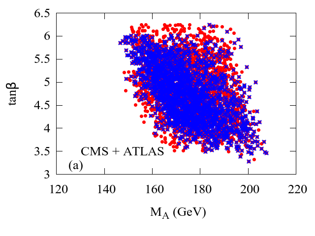
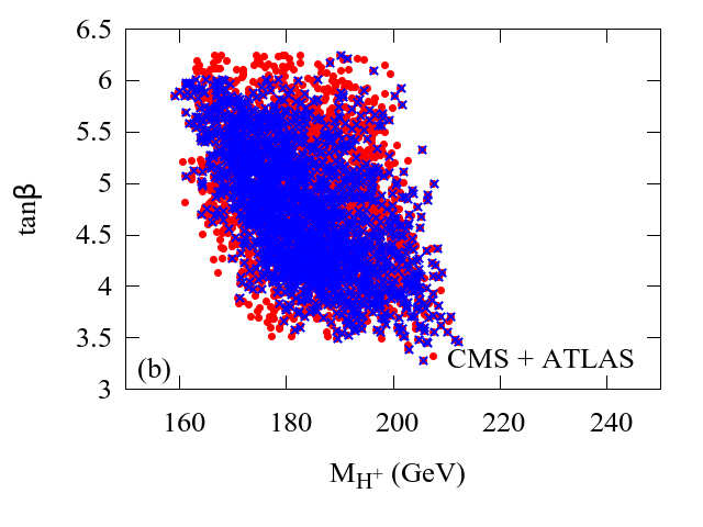
Figure 1: Scatter plot in the $M_{A}-\tan\beta$ (left) and $M_{H^{\pm}}-\tan\beta$ (right) plane. The red circles represent the points which satisfy all the constraints (Eqs. 1-6 ), while blue crosses display points which in addition satisfies the DM relic density constraint of Eq. 7.

In Fig. 2, we show the distribution of $\sigma\times{\rm BR}(\Phi\to\tau^{+}\tau^{-})$ where $\Phi\equiv h,A$, with respect to $M_{h}$ and $M_{A}$ for all the red circled points corresponding to Fig. 1, i.e., for those points which satisfy all the constraints (Eqs. 1-6) except Eq. 7. The black solid and blue dashed lines represent the CMS and ATLAS bounds respectively. The ggF production cross-section for both $h$ and $A$ increases with decrease of $\tan\beta$. However, the branching ratio of $h,A\to\tau^{+}\tau^{-}$ also gets reduced as $\tan\beta$ decreases. Thus, for low values of $\tan\beta$ as in the region of our interest, the product $\sigma(ggF)\times{\rm BR}(\Phi\to\tau^{+}\tau^{-})$ is still below the present experimental sensitivity, as can be seen from the left figures of both the upper and lower panels. However, when one considers the production mode of the Higgs boson in association with $b\bar{b}$, interestingly the present exclusion bounds are found to be very close to the model predictions. A better sensitivity in the $b\bar{b}$-fusion channel results in strong bounds on our parameter space. A sudden fall in $\sigma\times{\rm BR}(\Phi\to\tau^{+}\tau^{-})$ distribution near $M_{\phi}=190~{}{\rm GeV}$ originates from the opening of the dominant decay mode $A\to Z{h}$ ($m_{h}\sim 98~{}{\rm GeV}$ in our case) and consequent strong reduction in the branching ratio of $\Phi\to\tau^{+}\tau^{-}$. Thus, a closer look at these distributions reveals that one or two orders of improvement in the measurement of the quantity $\sigma\times{\rm BR}(\Phi\to\tau^{+}\tau^{-})$ for both the production processes will put strong constraint on the ILLH parameter space.

The allowed points in the present scenario correspond to the charged Higgs boson mass lying in the range 160 - 200 GeV. Thus, the dominant decay modes are seen to be $H^{\pm}\to\tau\nu_{\tau}$ and/or $H^{\pm}\to t\bar{b}$. Both the ATLAS and CMS collaborations have performed searches for the charged Higgs bosons with masses larger than that of the top quark [46, 47]. We find that the low $\tan\beta$ region with $M_{H^{\pm}}\geq 175$ GeV is consistent with the current LHC data.

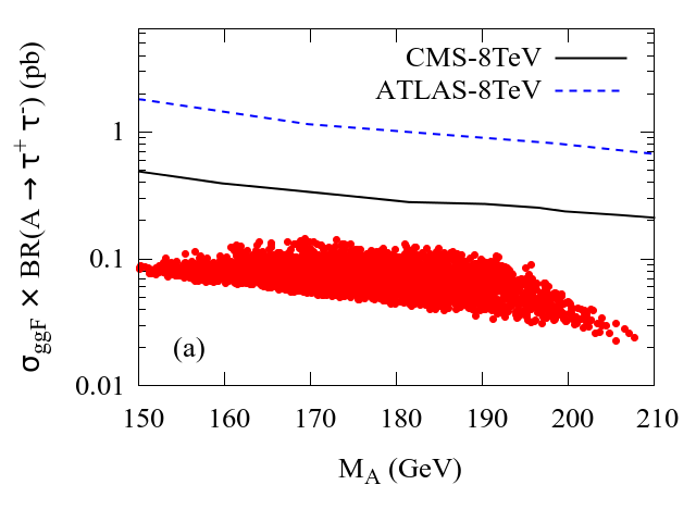
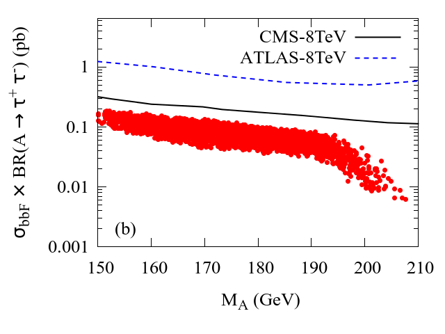
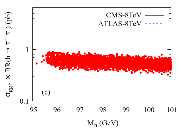
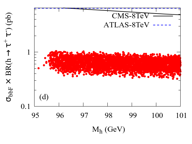
Figure 2: Distribution of $\sigma\times{\rm BR}(\Phi\to\tau^{+}\tau^{-})$ for all the red circled points corresponding to the Fig. 1, i.e., for those points which satisfy all the constraints (Eq.1-6) except the relic density bound of Eq.7. The black solid and blue dashed lines represent the CMS and ATLAS upper limits on this quantity. The upper and lower plots in the left panel assume Higgs is produced via ggF process, while bbF production mechanism is considered in the right panel. For details see text.

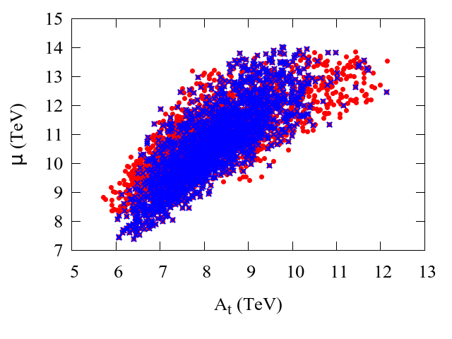
Figure 3: Plot in $A_{t}-\mu$ plane. The symbols carry the same meaning as in Fig. 1.

3.1 Light charged Higgs bosons and flavour data

Flavor observables play a crucial role in determining the valid regions of the MSSM parameter space. For example, rare B-decays that are helicity suppressed within the SM may on the other hand receive large contributions from the loop corrections involving SUSY particles. Two such rare B-decays are the radiative decay ${{\rm BR}(b\to s\gamma)}$ and the pure leptonic decay ${{\rm BR}(B_{s}\to\mu^{+}\mu^{-})}$. We will outline the relevant points of these constraints pertaining to our scenario with light $H^{\pm}$ while having large $\mu$ and large third generation of trilinear coupling parameters. We will particularly focus on the features of the valid parameter zones as allowed by the above constraints. In our analysis with positive $\mu$ and gluino mass ($M_{\tilde{g}}$) it turns out that the valid zones also have positive $A_{t}$. This may be seen in the $A_{t}-\mu$ plot of Fig. 3. The red circles represent the points which satisfy all the constraints of Eq. 1 to 6, while blue crosses indicate parameter points that additionally satisfy the DM relic density constraint of Eq. 7.

The experimental data of ${{\rm BR}(b\to s\gamma)}$ leaves a very small room for any Beyond the Standard Model (BSM) contribution. SUSY scenarios are effectively constrained by ${{\rm BR}(b\to s\gamma)}$ (which has both an upper and a lower limit) due to cancellation of relevant diagrams, when the individual SUSY contributions may become large. However, we will see the importance of next-to-leading order contributions in regard to this constraint. In the SM, the $t-W$ loops cause non-zero contributions to ${{\rm BR}(b\to s\gamma)}$, almost saturating the experimental value. In the MSSM, the dominant contributions to ${{\rm BR}(b\to s\gamma)}$ come from the $t-H^{\pm}$ and ${\tilde{t}}_{1,2}-{\tilde{\chi}}_{1,2}^{\pm}$ loops[48, 49], where the former type of loops comes with the same sign with that of the $t-W$ loops of the SM. Considering the contributions of ${\widetilde{\chi}_{1}}^{\pm}-\tilde{t}_{1}$ loops one has[50]:

$$\left.{{\rm BR}(b\to s\gamma)}\right|_{\chi^{\pm}}\propto\mu A_{t}\tan\beta f(m_{\tilde{t}_{{1}}},m_{\tilde{t}_{{2}}},m_{\tilde{\chi}^{+}})\frac{m_{b}}{v(1+\Delta m_{b})}.$$ (9)

On the other hand, for the $t-H^{\pm}$ loop contributions one finds[50]

$$\left.{{\rm BR}(b\to s\gamma)}\right|_{H^{+}}\propto\frac{\left(h_{t}\cos\beta-\delta h_{t}\sin\beta\right)}{v\cos\beta}\;g(m_{H^{+}},m_{t})\frac{m_{b}}{(1+\Delta m_{b})}.$$ (10)

Here $f$ and $g$ of Eqs. 9,10 are the loop functions. $\Delta m_{b}$ refers to the SUSY corrections to bottom mass where the SUSY QCD (SQCD) corrections may have a significant role which we will discuss soon. $\delta h_{t}$ as appearing in the second term of Eq. 10 principally results from the corrections to the top quark Yukawa coupling due to SQCD effects and this gives rise to a next-to-leading order (NLO) effect in ${{\rm BR}(b\to s\gamma)}$. The dominant SQCD corrections to $\delta h_{t}$ arising from the gluino-squark loops are given by[50],

$$\delta h_{t}=h_{t}\frac{2\alpha_{s}}{3\pi}\mu M_{\tilde{g}}\left(\cos^{2}\!\theta_{\tilde{t}}I(m_{\tilde{s}_{L}},m_{\tilde{t}_{2}},M_{\tilde{g}})+\sin^{2}\!\theta_{\tilde{t}}I(m_{\tilde{s}_{L}},m_{\tilde{t}_{1}},M_{\tilde{g}})\right),$$ (11)

where $I$ is again a loop function and $\theta_{\tilde{t}}$ is the squark mixing angle for the third generation.

Coming to the SQCD corrections to $\Delta m_{b}$ we have two types of contributions namely, from the ${b-\tilde{g}}$ and ${\widetilde{\chi}_{1}}^{\pm}-t$ loops[51, 52, 53, 54, 55]. Following Ref.[52] the corrections are given as below.

$$\Delta m_{b}\simeq\frac{2\alpha_{s}}{3\pi}M_{\tilde{g}}(\mu\tan\beta-A_{b})I(m_{\tilde{b}_{1}},m_{\tilde{b}_{2}},M_{\tilde{g}})+\frac{h_{t}^{2}}{16\pi^{2}}\mu(A_{t}\tan\beta-\mu)I(m_{\tilde{t}_{1}},m_{\tilde{t}_{2}},\mu).$$ (12)

One finds that over the parameter space scanned, the next-to-leading order (NLO) effects arising from the SQCD corrections of the top Yukawa coupling (gluino-squark loop diagrams) that in turn affects the contributions from the $t-H^{\pm}$ loops may have significant role in ${{\rm BR}(b\to s\gamma)}$. Typically, these NLO corrections are known to be important for large values of ${\rm tan}\beta$. But in spite of $\tan\beta$ being small in our analysis, the same corrections are also very important because of possible large values of $\mu$[51] considered in this work. The reason is that these NLO corrections are approximately proportional to $\mu M_{\tilde{g}}\tan\beta$[50, 51]. Thus, regions of parameter space with large values of $\mu$ may change the $\bar{t}bH^{+}$ coupling leading to reduction of $t-H^{\pm}$ loop contributions to ${{\rm BR}(b\to s\gamma)}$ [50]. Furthermore, as seen in Eq. 12 the SQCD corrections to $\Delta m_{b}$ can be substantially large in spite of the fact that $\tan\beta$ is small in our analysis. This will have an overall suppression effects of the aforesaid SUSY loop contributions to ${{\rm BR}(b\to s\gamma)}$ over the valid parameter space of interest with large and positive values of $\mu$ and $A_{t}$. We note that the valid regions of parameter space that satisfy ${{\rm BR}(b\to s\gamma)}$ correspond to heavy enough SUSY spectra and do not involve cancellation between the two basic types of SUSY loop diagrams. We have further imposed the constraint from ${{\rm BR}(B_{s}\to\mu^{+}\mu^{-})}$ [56, 57] in this analysis. In the parameter space that survives after imposing the constraint from ${{\rm BR}(b\to s\gamma)}$ it turns out that, ${{\rm BR}(B_{s}\to\mu^{+}\mu^{-})}$ does not take away any significant amount of parameter space because of its smaller SUSY contributions. This arises out of cancellation of relevant terms for the positive sign of $\mu A_{t}$ that gives rise to a positive value for the dimensionless Wilson coefficient of the semileptonic pseudoscalar operator (See Ref.[54] and references therein).

3.2 Benchmark points

Point	BP1	BP2
Input Parameters
$\tan\beta$	4.28	5.22
$\mu$ (GeV)	9333	9177
$M_{1}$ (GeV)	731.2	600.4
$M_{2}$ (GeV)	493.3	933.4
$M_{3}$ (GeV)	2056.7	3298
$A_{t}$ (GeV)	7047.2	6994.9
$A_{b}$ (GeV)	-4838.3	-2560.4
$M_{\tilde{Q}_{3L}}$(GeV)	1473.7	1522.8
$M_{\tilde{t}_{R}}$(GeV)	2806.9	3132.4
$M_{\tilde{b}_{R}}$ (GeV)	671.6	536.4
$m_{t}$ (GeV)	173.1	174.3

Table 2: Input parameters for the two benchmark points allowed by the constraints Eqs. 1-7.

Point	BP1	BP2
Mass spectrum
$M_{h}$ (GeV)	97.8	96.4
$M_{H}$ (GeV)	126.5	127.9
$M_{H^{\pm}}$ (GeV)	191.8	175.02
$M_{A}$ (GeV)	185.7	166.3
$m_{\tilde{g}}$ (GeV)	2230.6	3355.8
$m_{\tilde{t}_{1}}$ (GeV)	689.5	913.7
$m_{\tilde{t}_{2}}$ (GeV)	1409.2	2232.4
$m_{\tilde{b}_{1}}$ (GeV)	793.4	614.5
$m_{\tilde{b}_{2}}$ (GeV)	1560.9	1596.5
$m_{{\widetilde{\chi}_{1}}^{\pm}}$ (GeV)	492.9	933.0
$m_{\widetilde{\chi}_{1}^{0}}$ (GeV)	492.9	600.4
$m_{\widetilde{\chi}_{2}^{0}}$ (GeV)	731.1	933.0

Table 3: Mass spectrum for the two benchmark points.

Point	BP1	BP2
Values of the Observables
${{\rm BR}(b\to s\gamma)}\times 10^{4}$	3.65	3.85
${{\rm BR}(B_{s}\to\mu^{+}\mu^{-})}\times 10^{9}$	2.67	2.21
$\Omega_{\tilde{\chi}_{1}}h^{2}$	0.006	0.05
${\mu}^{H}_{gg}(\gamma\gamma)$	1.00	1.35
$\sigma_{\tilde{\chi}p}^{\rm SI}\times 10^{10}$ (pb)	1.27	0.07
${\mu}^{H}_{gg}(ZZ)$	0.93	1.31
${\mu}^{H}_{gg}(W^{+}W^{-})$	0.89	1.25
${\mu}^{H}_{Vh/H}(b\bar{b})$	0.57	0.49
${\mu}^{H}_{Vh/H}(\tau^{+}\tau^{-})$	1.23	1.38

Table 4: A few relevant observables for the two benchmark points considered in Table 3.

We show Tables 2-4 for the choice of two benchmark points (BP1 and BP2) allowed by the constraints from Eq. 1 to 7. Apart from the above constraints, large values of $\mu$ and $A_{t}$ in the valid region of parameter space specially motivate us in analyzing the effect of imposing the CCB constraints in a general setup going beyond the traditional constraints of CCB (see Ref.[45] and references therein for details) as used in the code SuSpect. We particularly analyze the above for only these two BPs rather than the entire parameter space simply for economy of computer time. We analyze the BPs by considering non-vanishing vacuum expectation values (vev) for the Higgs scalars and top-squarks. BP1 corresponds to a stable vacuum. BP2 has a cosmologically long-lived vacuum while allowing quantum tunneling. Moreover, the BPs are so chosen that the squark masses of the third generation lie above $\sim$ 600 GeV, sufficiently large to be safely above the current bounds from the LHC. For BP1 $m_{{\widetilde{\chi}_{1}}^{\pm}}\simeq m_{\widetilde{\chi}_{1}^{0}}$ and $\widetilde{\chi}_{1}^{0}$, which is the lightest SUSY particle (LSP) in our case, is almost wino-like. Thus, the mechanisms which lead to right relic density of the DM are mainly $\widetilde{\chi}_{1}^{0}-{\widetilde{\chi}_{1}}^{\pm}$ coannihilation and ${\widetilde{\chi}_{1}}^{\pm}$ mediated $\widetilde{\chi}_{1}^{0}$ pair-annihilation to $W^{\pm}$. The strong annihilation and coannihilations make the LSP underabundant. $m_{{\widetilde{\chi}_{1}}^{\pm}}$ is taken to be above 270 GeV so as to be consistent with the results from the disappearing charged tracks searches at the LHC (which impose a lower limit of 270 GeV for the masses of the wino-like LSPs[58]). The LSP in BP2 is predominantly a bino. The main annihilation mechanism in this case is the annihilation of sbottom pairs into a pair of gluons in the final state. The spin-independent $\widetilde{\chi}_{1}^{0}$-proton scattering cross-section $\sigma_{\tilde{\chi}p}^{\rm SI}$ is also seen to be well below the limit provided by the LUX experiment in both the cases. The smallness of $\sigma_{\tilde{\chi}p}^{\rm SI}$ arise as a result of large values of $\mu$ considered in this study leading to a negligible higgsino component within the LSP [59].

4 Prospects at the high luminosity run of the LHC

In the last section we studied the available parameter space in the MSSM consistent with the ILLH scenario and also provided with two benchmark points allowed by the LHC as well as low energy physics data. In this section, we proceed to discuss the sensitivity of the high luminosity run of the LHC to probe the ILLH scenario. We start with the possibility to discover/exclude a 98 GeV Higgs boson produced through the vector boson fusion (VBF) and Higgsstrahlung processes. Note that, the reason behind our choice of the two above-mentioned processes is that the Higgs boson production cross-section is directly proportional to the Higgs to gauge boson coupling $\sin^{2}({\beta-\alpha})$. Moreover, to satisfy the LEP excess we require $\sin^{2}({\beta-\alpha})\sim$0.2. Thus, if we observe a Higgs boson with mass $\sim$ 100 GeV in the associated/VBF processes with cross-sections $\sim$ 20% of the SM cross-section, that can be thought of as a smoking gun signal of the ILLH scenario. Furthermore, we also analyze how the future precision measurements of various Higgs signal strength variables may be used as an indirect probe for the ILLH scenario.

4.1 Direct search: 1. Vector boson fusion process

The Vector Boson Fusion (VBF) process, $pp\to jjH$, (where $j$ stands for light jets) is one of the most promising channels for the measurement of various properties of the observed 125 GeV Higgs boson at the LHC. It is a t-channel scattering process of two initial-state quarks with each one radiating a $W/Z$ which further annihilates to produce a Higgs boson. Characteristic features of this process are the presence of two energetic jets with a large rapidity gap along with a large invariant mass and the absence of a significant amount of hadronic activity in the central rapidity region. Even though the ggF process is the dominant production mechanism for the Higgs boson, due to the above distinctive features, VBF is sensitive enough to a precise measurement of various properties of the observed Higgs boson.

The ATLAS collaboration estimated the sensitivity of the VBF process for low mass Higgs bosons ($M_{H}<130$ GeV), where $H\to\tau^{+}\tau^{-}$ decay mode was considered at the 14 TeV LHC [60]. In the present work we perform a collider analysis following the ATLAS simulation to probe the discovery potential of the 98 GeV Higgs boson at the LHC-14. The ATLAS simulation considered three different decay modes of $\tau$, namley $\tau_{\ell}\tau_{\ell}$, $\tau_{\ell}\tau_{h}$, $\tau_{h}\tau_{h}$ where $\tau_{\ell}$ and $\tau_{h}$ denote the leptonically and hadronically decaying $\tau$-leptons respectively. From their analysis it is evident that the $\tau_{\ell}\tau_{h}$ channel has the best sensitivity compared to the other two possible modes (see Fig. 16 of Ref. [60]). Thus, in this work we confine ourselves in the $\tau_{\ell}\tau_{h}$ channel only. Note that, even though we follow the ATLAS simulation for our analysis, we further vary the selection cuts to optimize the signal to background ratio.

In order to tag the $\tau$-leptons as $\tau$-jets, we first identify $\tau$ through its hadronic decays and then demand that the candidate jet must have $|\eta|<$ 2.5 and $p_{T}>$ 30 GeV. Besides, the jet must also contain one or three charged tracks with $|\eta_{\rm track}|<$ 2.5 with the highest track $p_{T}>$ 3 GeV. To ensure proper charged track isolation, we additionally demand that there are no other charged tracks with $p_{T}>$ 1 GeV within the candidate jet. The di-tau invariant mass is calculated using the “collinear approximation technique” assuming the $\tau$-lepton and its decay products to be collinear [61] and the neutrinos to be the only source of $E{\!\!\!/}_{T}$. Neglecting the $\tau$ rest mass, the di-tau invariant mass can be written as,

$$m^{2}_{\tau\tau}=2(E_{h}+E_{\nu h})(E_{\ell}+E_{\nu\ell})(1-\cos{\theta_{\ell h}}),$$ (13)

where $E_{h}$ and $E_{\ell}$ represent the total energy of the hadronically and leptonically decaying $\tau$s respectively, while $\theta_{\ell h}$ represents the azimuthal angle between the directions associated with the above two decay modes of the $\tau$-lepton. We can now introduce two dimensionless variables $x_{\ell}$ and $x_{h}$, the fraction of $\tau$’s momentum taken away by the visible decay products, and rewrite the di-tau invariant mass as follows (with $x_{\ell,h}>0$).

$$m_{\tau\tau}=\frac{m_{\ell h}}{\sqrt{{x_{\ell}}{x_{h}}}},$$ (14)

where $m_{\ell h}$ is the invariant mass of the visible $\tau$-decay products, and

$$x_{h}=\frac{E_{h}}{(E_{h}+E_{\nu h})},\quad x_{l}=\frac{E_{l}}{(E_{l}+E_{\nu l})}.$$ (15)

Our event selection prescription involves four independent parameters which we vary in order to optimize the signal significances. These are the minimum transverse momentum $p_{T}$ of the hadronic $\tau$-lepton ($p^{\tau_{h}}_{T}$), minimum missing transverse energy ($E{\!\!\!/}_{T}^{\rm min}$), minimum transverse momentum of the two leading jets ($P^{\rm min}_{T,j}$) and minimum of the di-jet invariant mass ($m^{\rm min}_{j_{1}j_{2}}$). We proceed in the following steps.

• C1: We demand the presence of exactly one lepton (electron or muon) with $p^{e}_{T}>25$ GeV or $p^{\mu}_{T}>20$ GeV.

• C2: We identify hadronic $\tau$ with $p_{T}>p^{\tau_{h}}_{T}$ and charge opposite to that of the identified lepton.

• C3: We select events with missing transverse energy $E{\!\!\!/}_{T}$ greater than $E{\!\!\!/}_{T}^{\rm min}$.

• C4: The variables associated to di-tau invariant mass reconstruction satisfy $0\leq x_{l}\leq 0.75$, $0\leq x_{h}\leq 1$, and $\cos{\Phi_{lh}}\geq$ -0.9.

• C5: A cut on the transverse mass($m_{T}$) of the lepton and $E{\!\!\!/}_{T}$ is applied to suppress the $W+{\rm jets}$ and $t\bar{t}$ backgrounds, where

  $$m_{T}^{2}=2p_{T}^{l}E{\!\!\!/}_{T}(1-\cos{\Delta\Phi}),$$ (16)

  with $p_{T}^{\rm lep}$ representing the transverse momentum of the lepton and $\Delta\Phi$ is the angle between that lepton and $E{\!\!\!/}_{T}$ in the transverse plane. We demand $m_{T}<$ 30 GeV.

• C6: We require the leading two jets to satisfy $p_{T}\geq$ $p^{\rm min}_{T,j}$.

• C7: The forward jets should lie in opposite hemispheres $\eta_{j_{1}}\times\eta_{j_{2}}\leq$ 0 with tau centrality ${\rm min}({\eta_{j_{1}},\eta_{j_{2}}})\leq\eta_{{\rm lep},{\tau}}\leq{\rm max}({\eta_{j_{1}},\eta_{j_{2}}})$ for the two highest $p_{T}$ jets.

• C8: Forward jets should also satisfy $\Delta\eta_{j_{1}j_{2}}\geq$ 4.4 and di-jet invariant mass $m_{j_{1}j_{2}}\geq$ $m^{\rm min}_{j_{1}j_{2}}$.

• C9: The events are rejected if there are any additional jets with $p_{T}\geq$ 20 GeV with $|\eta|\leq$ 3.2.

• C10: Finally, we select the events with di-tau invariant mass satisfying 90 GeV $\leq$ $m_{\tau\tau}\leq$ 110 GeV.

Signal Regions	$p^{\tau_{h}}_{T}$	$E{\!\!\!/}_{T}^{\rm min}$	$p^{{\rm min}}_{T,j}$	$m^{\rm min}_{j_{1}j_{2}}$
SR0	20.0	30.0	20.0	700.0
SRA	80.0	80.0	60.0	1200.0
SRB	50.0	50.0	40.0	1500.0

Table 5: Details of the different signal regions are given. The kinematic selection cuts obtained from the ATLAS simulation is denoted by SR0, while our optimized selection cuts are described by SRA and SRB. For details see the text.

The possible SM backgrounds in this case come from $t\bar{t}+{\rm jets}$, $W+{\rm jets}$, $Z+{\rm jets}$ and di-boson final states ($WW$, $ZZ$, $WZ$). From the ATLAS simulation [60], we find that $Z+{\rm jets}$ is the most dominant background with $Z\to\tau^{+}\tau^{-}$. Hence, in our analysis, we simulate only the $Z+{\rm jets}$ background. We use MADGRAPH5 (v1 2.2.2) [62] to generate the background events and then hadronize the events using PYTHIA (version 6.4.28) [63]. Table 5 shows the optimized set of cuts. The expected number of signal and background events at the 14 TeV run of the LHC with 3000 ${\rm fb}^{-1}$ of integrated luminosity within a mass window of 90-110 GeV and the resulting statistical significances for three optimized scenarios are presented in Table 6. We obtain a maximum of 1.9$\sigma$ significance for the signal region SRA with 3000 ${\rm fb}^{-1}$ of data. Note that, we have considered only the dominant background $Z+{\rm jets}$. However, we expect the significances to be reduced even further if we consider all the possible backgrounds. Thus, we conclude that the possibility of observing the 98 GeV Higgs boson via VBF process at the 14 TeV LHC run is rather poor even at an integrated luminosity of $3000~{}{\rm fb}^{-1}$.

	SR0	SRA	SRB
Signal (S)	271.3	25.4	71.0
Backgounds (B)	1713.3	55.3	221.1
Significance ($\mathcal{S}={S\over\sqrt{B+\kappa^{2}B^{2}}}$)	0.78	1.91	1.52

Table 6: Expected number of events at the 14 TeV LHC with 3000 ${\rm fb}^{-1}$ of integrated luminosity within a mass window 90 - 110 GeV for individual signal and total background. We assume that the signal cross section is 20% of the SM value calculated with the Higgs mass $m^{\rm SM}_{h}$ = 98 GeV. The signal significances are calculated using systematic uncertainty $\kappa=0.2$.

4.2 Direct search: 2. Associated production

Another important production mode of the 98 GeV Higgs boson is the Higgs-strahlung process where the Higgs is produced in association with a gauge boson $W/Z$. In our earlier work [9], we discussed the discovery potential of the 98 GeV Higgs boson produced via this process giving special attention to the boosted regime with the assumption that it was produced with $p_{T}>200$ GeV. It is pertinent to note that in Ref.[9] we took the number of background events directly from the ATLAS simulation [64]. However, in this work, we perform a more detailed Monte Carlo simulation by generating both the signal and background events and then optimizing the event selection cuts. We again focus on the boosted regime here. Note that, even though the production cross-section is very small in this highly boosted regime ($p_{T}$ of the Higgs is greater than 200 GeV), relatively large kinematic acceptance and large background reduction make this analysis special. The details of our collider analysis can be found in Ref. [9]. However, we give a very brief outline of our analysis below. We divide this part of our analysis into three categories based on the decay modes of the gauge bosons, namely,

1. $Wh$ process with $W$ decaying leptonically with missing transverse momentum $p{\!\!\!/}_{T}>p{\!\!\!/}_{T}^{\rm min}$ and $p_{T}^{e/\mu}>30$  GeV. The transverse momentum of the $W$-boson must also satisfy $p_{T}>p_{T,W}^{\rm min}$. Here we vary the quantities $p{\!\!\!/}_{T}^{\rm min}$ and $p_{T,W}^{\rm min}$ independently.

2. $Zh$ process with $Z$ decaying into a pair of leptons (e/$\mu$) with di-lepton invariant mass satisfying $80~{}{\rm GeV}<m_{\ell\ell}<100$ GeV while $p^{Z}_{T}$ exceeds certain minimum value $p_{T,Z}^{\rm min}$. We also vary the transverse momentum of the two leptons independently.

3. Finally, missing transverse energy driven signal with no leptons and $E{\!\!\!/}_{T}>E{\!\!\!/}_{T}^{\rm min}$. This kind of signature mainly comes from the process $Zh$ when $Z$-boson decays invisibly to a pair of neutrinos. However, contributions from $Wh$ process may also come when the lepton from $W$ remains undetected.

In the above, $p_{T}^{\rm min}$ refers to the minimum $p_{T}$ of the Higgs required to claim the jet to be a Fat jet with $|\eta|<$ 2.5. Similar to our VBF analysis, we first analyze the ATLAS optimized cuts and then vary some of the important observables relevant to a specific process so as to obtain the maximum sensitivity of the given channel. For example, for the $\ell^{+}\ell^{-}b\bar{b}$ channel we vary the transverse momentum of the Higgs jet, $Z$ boson and the pair of leptons to get the maximum signal significance. Similar strategy has been opted for other modes. The default selection cuts for a given channel have been denoted as “SR0”, while our optimized selection cuts are represented as “SRA”, “SRB” and “SRC” for the $\ell^{+}\ell^{-}b\bar{b}$, $\ell^{+}\nu_{\ell}b\bar{b}$ and $E{\!\!\!/}_{T}b\bar{b}$ signals respectively (see Table 7). We use PYTHIA (version 6.4.28)[63] for generation of signal events while FASTJET (version 3.0.3)[65] is used for reconstruction of jets and also implementation of the jet substructure analysis. The most dominant SM backgrounds for our process of interest are $WW$, $ZZ$, $WZ$, $Wb\bar{b}$, $Zb\bar{b}$ and $t\bar{t}$. We use MADGRAPH to generate the $Wb\bar{b}$, $Zb\bar{b}$ samples and then passed them to PYTHIA for showering and hadronization while the rest of the background samples are generated using PYTHIA itself.

We present our final results in Table 8 where we scale the cross-sections by 0.2 and focus in the mass window 90 - 110 GeV to satisfy the 2.3$\sigma$ LEP excess. In Table 8 we display the expected number of events for the signal and various backgrounds with 3000 ${\rm fb}^{-1}$ of luminosity. The statistical significances for the signal regions SR0 (the default ATLAS parameters) as well as SRA, SRB and SRC (our optimized sets) are also shown for the three possible decay modes. We find that the best sensitivity comes from the channel $\ell^{+}\ell^{-}b\bar{b}$ with 2.6$\sigma$ significance, while $\ell^{+}\nu_{\ell}b\bar{b}$ and $E{\!\!\!/}_{T}b\bar{b}$ have statistical significances of 2.5$\sigma$ and 1.5$\sigma$ respectively. We must note that although we assume 20% systematic uncertainty (i.e., $\kappa$ = 0.2), nevertheless with 3000 ${\rm fb}^{-1}$ of luminosity we can expect to have a better control over the various sources of systematic uncertainties leading to an enhanced signal significance. Therefore, one can expect to marginally exclude the 98-125 GeV Higgs scenario using 3000 ${\rm fb}^{-1}$ of data at the 14 TeV LHC via the Higgstrhlung process.

Process	Signal Regions	Selection Cuts
		$p^{\rm min}_{T,Z}$	$p^{\rm min}_{T,j_{1}}$	$\Delta\Phi_{1}$	$p^{\ell_{1}}_{T}$	$p^{\ell_{2}}_{T}$
$\ell^{+}\ell^{-}b\bar{b}$	SR0	180	200	1.2	25	20
	SRA	250	250	1.2	100	50
		$p^{\rm min}_{T,W}$	$p^{\rm min}_{T,j_{1}}$	$\Delta\Phi_{1}$	$p{\!\!\!/}_{T}^{\rm min}$
$\ell^{+}\nu_{\ell}b\bar{b}$	SR0	180	200	1.2	30
	SRB	300	300	1.5	75
		$p^{\rm min}_{T,j_{1}}$	$\Delta\Phi_{1}$	$p{\!\!\!/}_{T}^{\rm min}$
$E{\!\!\!/}_{T}b\bar{b}$	SR0	200	1.2	200
	SRC	250	1.5	300

Table 7: Different signal regions for the three processes considered in this analysis. The default ATLAS simulation is denoted by SR0, while our optimized selection cuts are described by SRA, SRB and SRC for the three processes.

Process	Signal Region	Signal (S)	Background (B)	Significance ($S\over\sqrt{B+\kappa^{2}B^{2}}$)
$\ell^{+}\ell^{-}b\bar{b}$	SR0	184.9	956.1	0.95
	SRA	94.8	168.7	2.62
$\ell\nu b\bar{b}$	SR0	360.2	1998.4	0.89
	SRB	99.5	185.8	2.51
$E{\!\!\!/}_{T}b\bar{b}$	SR0	184.9	2614.3	0.35
	SRC	94.8	297.2	1.53

Table 8: Expected number of events at the 14 TeV LHC run with 3000 ${\rm fb}^{-1}$ of integrated luminosity within a mass window of 90 - 110 GeV for the individual signal and the combined background processes assuming 20% LEP excess in this region of interest.

4.3 Indirect search: Higgs coupling measurements

Precise measurement of the various Higgs signal strength variables can prove to be significant to indirectly probe/exclude the ILLH scenario. We find that the important observables which can play crucial roles in this regard are ${\mu}_{bb}$, ${\mu}_{\tau\tau}$ and ${\mu}_{ZZ}$ for a given production mechanism of the observed 125 GeV Higgs boson. Before going into a detailed analysis of these observables, let us first discuss some of the important Higgs boson couplings. The tree level Yukawa coupling of the bottom quark with the heavy Higgs boson of the MSSM having a mass around 125 GeV goes as $\cos\alpha\over\cos\beta$ where $\tan\beta$ is the ratio of the vevs of the two Higgs doublets. However, loop corrections (in orders of $\alpha_{s}\tan\beta$) involving various supersymmetric particles can significantly modify the tree level $Hb\bar{b}$ Yukawa coupling. These effects are generally denoted by the quantity $\Delta_{b}$ and the additional contribution coming from $\Delta_{b}$ can be summarized as [51, 66, 67, 68],

$$\epsilon=\biggl{(}{1\over 1+\Delta_{b}}\biggr{)}\times\biggl{(}1+{\Delta_{b}\cot\beta\tan\alpha}\biggr{)}.$$ (17)

In the left panel of Fig. 4, we show the dependence on $\Delta_{b}$ of the quantity $\epsilon$ which estimates the loop contribution to the tree level Yukawa coupling. We find that the effect of $\Delta_{b}$ is indeed significant in the parameter space of our interest. In the right panel of Fig. 4, we show the variation of the complete $Hb\bar{b}$ coupling (the effect of $\Delta_{b}$ included) with the tree level coupling. It is evident from both the figures that for a significant number of points $\Delta_{b}$ is indeed large. Thus, even though the maximum value of the tree level coupling goes up to 1.4-1.5, the total $Hb\bar{b}$ coupling never exceeds unity, implying that the $Hb\bar{b}$ coupling is always suppressed with respect to the SM expectation which can indeed serve as a very distinctive feature of the ILLH scenario.

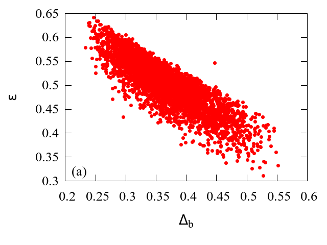
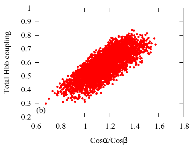
Figure 4: Left panel shows the distribution of the quantity $\epsilon=\biggl{(}{1\over 1+\Delta_{b}}\biggr{)}\times\biggl{(}1+{\Delta_{b}\cot\beta\tan\alpha}\biggr{)}$ with the variation of $\Delta_{b}$. The variation of the total Yukawa coupling of the bottom quark with the heavier Higgs boson with respect to the tree level coupling $\frac{\cos\alpha}{\cos\beta}$ is shown in the right panel.

Let us now turn our attention to another important decay mode $H\to ZZ^{*}$. In the left panel of Fig. 5, we show the variation of the ratio $\Gamma_{ZZ}/\Gamma_{ZZ}^{SM}$ to the square of the tree level $HZZ$ coupling $\sin({\beta-\alpha})$. Here, $\Gamma_{ZZ}$ denotes the partial width of the decay $H\to ZZ^{*}$ in the MSSM and $\Gamma_{ZZ}^{SM}$ denotes the same for the SM. The behaviour is well understood; as the coupling decreases so does the partial width. However, we must note that the $H\to ZZ^{*}$ partial width is also suppressed in this case. With both the partial widths for the decays $H\to b\bar{b}$ and $H\to ZZ^{*}$ suppressed, one can expect to observe a significant suppression in the total decay width of the Higgs boson as well. From the plot in the right panel of Fig. 5, where the X-axis denotes the ratio $\Gamma_{ZZ}/\Gamma_{ZZ}^{SM}$ and the Y-axis stands for the ratio of the total Higgs decay width ($\Gamma_{tot}$) in the MSSM to that in the SM ($\Gamma_{tot}^{SM}$), one can easily observe the suppression in the total decay width. Thus, one may also expect to find a mild enhancement in partial widths of the sub-dominant decay modes like $\tau^{+}\tau^{-}$, $gg$.

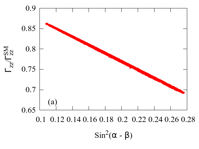
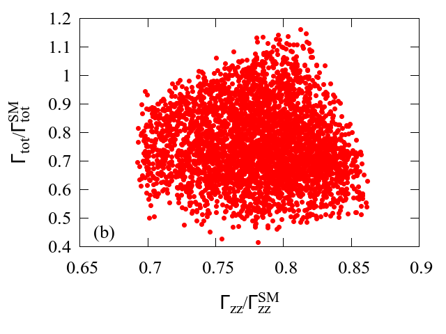
Figure 5: The correlation of the partial decay width of Higgs to $ZZ^{*}$ decay with $\sin^{2}({\beta-\alpha})$ (Left panel) and with total Higgs decay width $\Gamma_{tot}$ (Right panel).

Improved measurement of the signal strength variables at the high luminosity run of the LHC may help us to probe the ILLH scenario indirectly. We present a detailed study in this regard as follows. We have already introduced the signal strength variables in Sec. 2. Here, we discuss the variables which we find interesting and which are seen to have some impact to probe/exclude the parameter space of our interest. In the left-most panel of Fig. 6, we display the correlation in the ${\mu}^{ZZ}_{ggF}-{\mu}^{bb}_{VBF}$ plane. We assume gluon-gluon fusion (ggF) process as the production mechanism for the Higgs boson decaying into $ZZ$ while for the final state $b\bar{b}$ the Higgs is taken to be produced via vector-boson fusion (VBF) process. We find that although ${\mu}^{ZZ}_{ggF}$ can vary in the range 0.6 - 1.6, the values of ${\mu}^{bb}_{VBF}$ is seen to be suppressed i.e., less than unity. Furthermore, even though gluon-gluon fusion process is the dominant one, associated production mechanism of the Higgs can also be used to measure these signal strength variables. We discuss the correlations of three such variables, namely ${\mu}^{ZZ}_{VBF}$, ${\mu}^{bb}_{VBF}$ and ${\mu}^{\tau\tau}_{VBF}$. In the middle and right-most panel we show the correlations in the ${\mu}^{ZZ}_{VBF}-{\mu}^{bb}_{VBF}$ and ${\mu}^{ZZ}_{VBF}-{\mu}^{\tau\tau}_{VBF}$ planes respectively. Similar to the ggF case, there are no such restrictions on the values of ${\mu}^{ZZ}_{VBF}$. However, we find a strong anti-correlation between ${\mu}^{bb}_{VBF}$ and ${\mu}^{\tau\tau}_{VBF}$. The values of ${\mu}^{bb}_{VBF}$ is found to be always less than unity while those of ${\mu}^{\tau\tau}_{VBF}$ to be dominantly greater than unity. At this point, one might be interested to know the present status of the measurement of these Higgs signal strength correlations at the LHC. In Fig. 7, we study these correlations in the $\mu^{f}_{ggF+t\bar{t}H}$ - $\mu^{f}_{VBF+VH}$ plane for a generic final state $f$, and then compare the model predictions with the 95% correlation contours obtained using the 10-parameter fit for the five decay modes of the observed Higgs boson by the ATLAS and CMS combined 7 and 8 TeV data [31]. In the left panel, we show $\gamma\gamma$, $ZZ$ and $WW$ channels while right panel for $b\bar{b}$ and $\tau^{+}\tau^{-}$. The subscript ‘F’ denotes the combined ggF and $t\bar{t}H$ process, while ‘V’ signifies the combined VBF and VH processes. However, here for the “fusion” (F) mode we consider ggF only as Higgs production via ggF is much larger compared to the $t\bar{t}H$ process. Comparing the correlation plots (Fig. 7) with Table 1, we find that at present the impact of these correlations at the parameter space of interest is comparable with that of the individual signal strengths (less than 2% points are found to be outside the 95% C.L. contours). However, here we would like to note that with precise measurements in the future runs of LHC these contours are expected to shrink, this may lead to interesting consequences for our model parameter space. Considering the future improvements in signal strength measurements, if we assume that at the high luminosity run of the LHC with 3000 ${\rm fb}^{-1}$ of data ${\mu}^{ZZ}_{VBF}$ can be measured with an accuracy at the level of 30%, then from these correlations we can infer that ${\mu}^{\tau\tau}_{VBF}$ will always have values larger than unity. However, ${\mu}^{bb}_{VBF}$ will be less than 0.8. Thus, for a given measurement of the signal strength variable in the $ZZ$ channel, observation of suppression of the same quantity for the $b\bar{b}$ channel and enhancement in the $\tau\tau$ channel will be an ideal probe of the ILLH scenario.

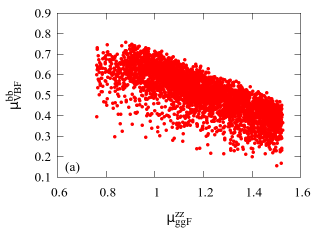
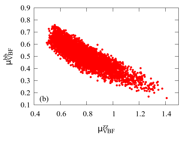
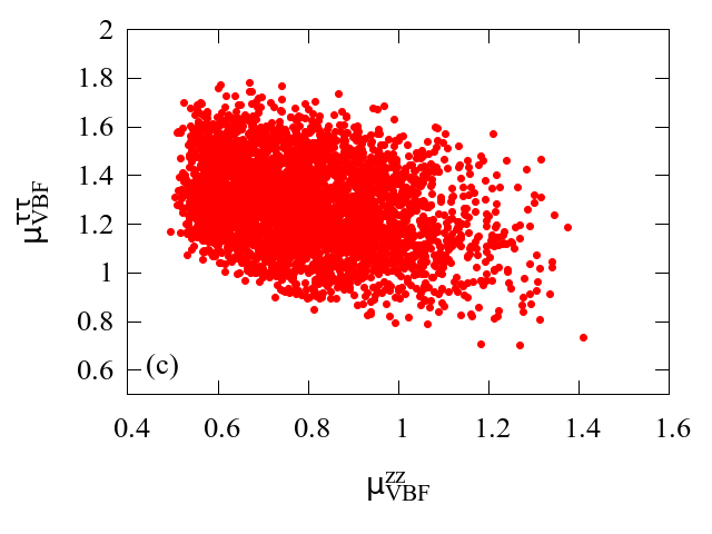
Figure 6: Correlation plots in ${\mu}^{ZZ}_{ggF}-{\mu}^{bb}_{VBF}$ (left), ${\mu}^{ZZ}_{VBF}-{\mu}^{bb}_{VBF}$ (middle) and ${\mu}^{ZZ}_{VBF}-{\mu}^{\tau\tau}_{VBF}$ (right) planes. For details see the text.

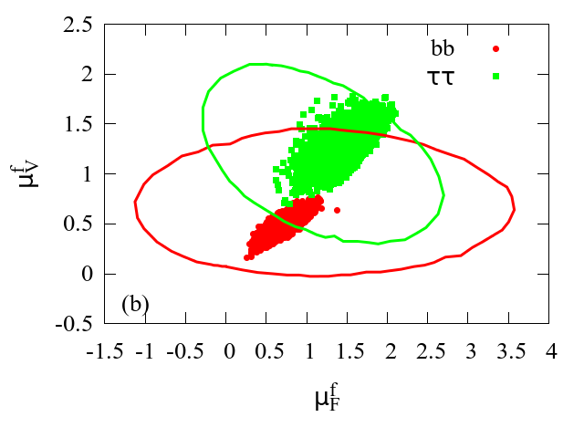
Figure 7: The 95% C.L. contours in the $\mu^{f}_{ggF+t\bar{t}H}$ - $\mu^{f}_{VBF+VH}$ plane with the ATLAS and CMS combined 7 and 8 TeV data for five possible decay modes: in the left we show $\gamma\gamma$, $ZZ$ and $WW$ channels while right panel for $b\bar{b}$ and $\tau^{+}\tau^{-}$. The subscript ‘F’ denotes the combined ggF and $t\bar{t}H$ process, while ‘V’ signifies the combined VBF and VH processes. However, here for the “fusion” (F) mode we consider ggF only as Higgs production via ggF is much larger compared to the $t\bar{t}H$ process. See the text for more details.

Before we end this section, let us summarize our results from the collider analysis. We analyze the most important production mechanism of the 98 GeV Higgs boson, namely the VBF and associated production processes, and find that these processes are not sensitive enough to exclude the ILLH scenario. We then attempt to exclude this possibility indirectly using various Higgs signal strength variables, and here we find very distinctive features in the correlations of the signal strength variables for $bb$, $\tau\tau$ and $ZZ$ decay channels. However, there exists several other processes which can also be used directly to probe this scenario, e.g. the associated production of the 98 GeV Higgs boson with a pair of top quarks ($t\bar{t}h$). Even though this process do not directly involve the $\sin^{2}({\beta-\alpha})$ coupling, still it can be used to probe this scenario. In our earlier work [9], we performed a naive collider analysis of this process, following the same analysis for a SM Higgs boson [69], and obtained a 2.6$\sigma$ statistical significance without considering systematic uncertainties. A more detailed study is required, specially focusing on the boosted regime and applying the jet substructure technique, which is beyond the scope of the present work. Interestingly, we can also discover/exclude the 98-125 GeV Higgs scenario by looking for the other Higgses present in this model, e.g. the neutral CP-odd Higgs $A$ and the charged Higgs bosons $H^{\pm}$. One of the most important characteristic signatures of this ILLH scenario is the presence of relatively light $A$ and $H^{\pm}$ bosons with masses $\mathrel{\mathchoice{\vbox{\offinterlineskip\halign{$\m@th\displaystyle\hfil#\hfil$\cr<\crcr\sim\crcr} }}{\vbox{\offinterlineskip\halign{$\m@th\textstyle\hfil#\hfil$\cr<\crcr\sim\crcr} }}{\vbox{\offinterlineskip\halign{$\m@th\scriptstyle\hfil#\hfil$\cr<\crcr\sim\crcr} }}{\vbox{\offinterlineskip\halign{$\m@th\scriptscriptstyle\hfil#\hfil$\cr<\crcr\sim\crcr} }}}$ 200 GeV. The pseudoscalar Higgs $A$ is produced via gluon-gluon fusion and/or $b\bar{b}$ fusion process and, if kinematically allowed, can decay to $Zh$ giving rise interesting final state topologies involving multi-leptons and multiple b-jets. On the other hand, the charged Higgs bosons are produced by $tbH^{\pm}$ process and decays dominantly into $\tau\nu_{\tau}$ and $t\bar{b}$ final states. A dedicated analysis for these very light CP-odd and charged Higgses in the context of high luminosity run of the LHC is required. We leave this very interesting possibility for our future work. Thus, the observation of a charged Higgs and a pseudoscalar Higgs boson with masses between 140 - 200 GeV and simultaneously the non-observation of any CP-even Higgs in the same region will be a direct probe of the ILLH scenario. Furthermore, productions of these light Higgses in pair, e.g. processes like $H^{\pm}A$, $H^{+}H^{-}$, $H^{\pm}h$, $Ah$ are also very interesting possibilities at the LHC. There exists a study considering all of these processes at the LHC in the context of non-decoupling region of the MSSM [13]. However, the authors focused only on the regions with masses of these Higgses lying between 95 - 130 GeV. Note that, this 95 - 130 GeV region is already excluded by the pseudoscalar and charged Higgs searches at the LHC, and thus a study focussing on the region 140 - 200 GeV is now required which we plan to address in our future correspondence. We would like to mention that in our earlier work we discussed the possibility of observing the 98 GeV Higgs boson directly at the ILC. We found that the above could be easily discovered/excluded at the 250 GeV ILC with a 100 ${\rm fb}^{-1}$ of luminosity which is easily achievable within the first few years of its run. Finally we would like to add one important point regarding the direct measurement of various SUSY particles at the high luminosity (HL) run of LHC. The expected exclusion limits at the HL-LHC for the top and bottom squarks are around 1 TeV, for charginos and neutralinos around 600 GeV while for gluinos around 2.5 TeV [70]. We check that even with such a heavy sparticle spectrum, there is ample parameter space which satisfies the current LHC data, thus we conclude that it is almost impossible to exclude the 98-125 GeV scenario even at the high luminosity run of LHC.

5 Summary and conclusions

The objective of this work is to interpret the LEP excess observed around a mass of $\sim$ 98 GeV as the lighter CP-even Higgs boson of the MSSM while the LHC-observed scalar at $\sim$ 125 GeV plays the role of the heavier one. We analyze this scenario in the light of the latest results from the LHC including the limits on Higgs signal strengths. Other relevant constraints like those coming from the flavor sector e.g. ${{\rm BR}(b\to s\gamma)}$, ${{\rm BR}(B_{s}\to\mu^{+}\mu^{-})}$ and the DM relic density constraint are also taken into account. The ATLAS/CMS searches in the $H/A\rightarrow\tau^{+}\tau^{-}$ and charged Higgs searches restrict the values of $\tan\beta$ to a very narrow range. By performing a detailed random scan over the MSSM parameter space we try to pin point the region of parameter space where all the above constraints can be simultaneously accommodated. We observe that the ILLH scenario can still be harboured within the MSSM framework. The values of $\mu$ required to satisfy the above criteria are generically large $\mathrel{\mathchoice{\vbox{\offinterlineskip\halign{$\m@th\displaystyle\hfil#\hfil$\cr>\crcr\sim\crcr} }}{\vbox{\offinterlineskip\halign{$\m@th\textstyle\hfil#\hfil$\cr>\crcr\sim\crcr} }}{\vbox{\offinterlineskip\halign{$\m@th\scriptstyle\hfil#\hfil$\cr>\crcr\sim\crcr} }}{\vbox{\offinterlineskip\halign{$\m@th\scriptscriptstyle\hfil#\hfil$\cr>\crcr\sim\crcr} }}}$ 7 TeV and $A_{t}$ tends to assume only appreciably large positive values.

To perform the analysis in a model independent way we use the limits on $\sigma\times{\rm BR}(\Phi\rightarrow\tau^{+}\tau^{-})$, $\sigma$ being the production cross-section of the non-standard Higgs boson $\Phi$. The LHC limits are available for ggF and VBF production processes. We observe that $\sigma(ggF)\times{\rm BR}(\Phi\rightarrow\tau^{+}\tau^{-})$ lies well below the experimental limit for the small values of $\tan\beta$ considered in this analysis. However, the values of this observable for associated production with $b\bar{b}$ seems to be very close to the present experimental bound.

In the ILLH scenario that is associated with a light $H^{\pm}$, the constraint from ${{\rm BR}(b\to s\gamma)}$ plays an important role to eliminate a large region of parameter space. We remember that the associated SM contributions almost saturate the the experimental limit. Generally, the ${\widetilde{\chi}_{1}}^{\pm}-\tilde{t}_{1}$ loop contributions are not large enough to effectively cancel the contributions from the $H^{\pm}-t$ loops where $H^{\pm}$ is light. This causes a large amount of the parameter space to be discarded. It is only for large $\mu$ zone (with large $A_{t}$ values) along with sign$(\mu A_{t})>0$ the NLO contributions arising out of the top-quark Yukawa coupling partially cancel the leading order contributions of the $H^{\pm}-t$ loops. Additionally, there is an overall suppression coming out of SQCD corrections to the mass $m_{b}$. Thus the available parameter space that satisfies ${{\rm BR}(b\to s\gamma)}$ constraint has large values of $\mu$ with sign$(\mu A_{t})>0$. The other constraint namely ${{\rm BR}(B_{s}\to\mu^{+}\mu^{-})}$ is not a very stringent one in this zone of parameter space that survive the ${{\rm BR}(b\to s\gamma)}$ constraint.

An important result regarding the Higgs signal strength variables is obtained when we closely study the points satisfying all the constraints along with the limits on $R^{H}_{gg}(\gamma\gamma)$. If we further demand that values of $R^{H}_{gg}(ZZ)$ lie within 20% around the SM value of unity, all the points are seen to have $R^{H}_{VH}(bb)\mathrel{\mathchoice{\vbox{\offinterlineskip\halign{$\m@th\displaystyle\hfil#\hfil$\cr<\crcr\sim\crcr} }}{\vbox{\offinterlineskip\halign{$\m@th\textstyle\hfil#\hfil$\cr<\crcr\sim\crcr} }}{\vbox{\offinterlineskip\halign{$\m@th\scriptstyle\hfil#\hfil$\cr<\crcr\sim\crcr} }}{\vbox{\offinterlineskip\halign{$\m@th\scriptscriptstyle\hfil#\hfil$\cr<\crcr\sim\crcr} }}}0.8$. As already mentioned, the loop correction to bottom quark Yukawa coupling and hence to bottom quark mass ($\Delta m_{b}$) is significantly large in the present case. This reduces the partial decay width $\Gamma_{(H\rightarrow b\bar{b})}$. The value of $\Gamma_{(H\rightarrow ZZ)}$ is also small, leading to a reduction in the total decay width. However, the ${\rm BR}(H\rightarrow ZZ)$ can be significantly large. Thus, for the points with $0.8<R^{H}_{gg}(ZZ)<1.2$ the value of $R^{H}_{VH}(bb)$ is seen to be $\mathrel{\mathchoice{\vbox{\offinterlineskip\halign{$\m@th\displaystyle\hfil#\hfil$\cr<\crcr\sim\crcr} }}{\vbox{\offinterlineskip\halign{$\m@th\textstyle\hfil#\hfil$\cr<\crcr\sim\crcr} }}{\vbox{\offinterlineskip\halign{$\m@th\scriptstyle\hfil#\hfil$\cr<\crcr\sim\crcr} }}{\vbox{\offinterlineskip\halign{$\m@th\scriptscriptstyle\hfil#\hfil$\cr<\crcr\sim\crcr} }}}0.8$. This can play a major role as a distinctive feature of the present scenario provided the sensitivity on the coupling strength measurements is increased to a desired accuracy.

We analyze the possibilities of observing the ILLH scenario in the 14 TeV run of the LHC in two production channels, the vector boson fusion process and associated production with $W/Z$ boson. For the VBF process we follow the ATLAS simulation for the decay mode $H\rightarrow\tau_{l}\tau_{h}$. The selection cuts are varied to obtain an optimum signal to background ratio. We simulate only the $Z$ + jets events as the dominant SM background in this analysis. From statistical significances of the three optimized scenarios considered here we conclude that the possibility of observing the ILLH scenario with 3000 ${\rm fb}^{-1}$ of luminosity is rather small.

For the Higgstrahlung processes we concentrate on the highly boosted regime where the Higgs boson of mass 98 GeV is produced with $p_{T}>$ 200 GeV. Three different scenarios are considered here depending on the decays of the associated gauge boson. These are the $WH$ process with $W$ decaying leptonically, the $ZH$ process with $Z$ decaying to $e/\mu$ pair, the $ZH$ process with invisible decays of the $Z$ boson. We generate both the signal and background events through a detailed Monte Carlo simulation following the ATLAS analysis. The results are presented for three optimized selection regions along with the one using default selection cuts. From the results we observe that the ILLH scenario can be marginally ruled out with 3000 ${\rm fb}^{-1}$ of luminosity at the 14 TeV run of the LHC.

Finally, we summarize our findings of the 98 - 125 GeV ILLH scenario as follows:

• The most updated LHC data along with the low energy physics flavor data and bounds from dark matter searches does not exclude the possibility of having a 98 - 125 GeV Higgs scenario. We provide two sample benchmark points in support of our results.

• The possibility for direct detection of the 98 GeV Higgs boson at the run-2 of the LHC is marginal even after using the state-of-the-art jet substrcuture technique.

• However precise measurements of the Higgs signal strengths may act as an indirect probe of the ILLH scenario. We find interesting correlations between these signal strength variables. For example, the quantity $R_{b\bar{b}}$ is always less that unity, thus we find that if we can measure the Higgs signal strength associated to the Higgs decay to $ZZ$ then we must see a strong suppression in the $b\bar{b}$ mode. We expect at the high luminosity run of LHC these measurements will be improved by few orders of magnitude, and thus could easily be used as a probe of the ILLH scenario.

Acknowledgments: The work of BB is supported by Department of Science and Technology, Government of INDIA under the Grant Agreement numbers IFA13-PH-75 (INSPIRE Faculty Award). AC would like to thank the Department of Atomic Energy, Government of India for financial support. MC would like to thank Council of Scientific and Industrial Research, Government of India for financial support. We gratefully acknowledge the help received from Abhishek Dey for running the code Vevacious for the benchmark points.

References

- [1] ATLAS Collaboration, Phys. Lett. B(716,1-29,2012); arXiv:1207.7214;CMS Collaboration, Phys. Lett. B(716,30-61,2012), arXiv:1207.7235
- [2] M. Flechl [ATLAS for and CMS Collaborations], arXiv:1503.00632
- [3] For reviews on supersymmetry, see, e.g., H. P. Nilles, Phys. Rep. 110, 1 ( 1984); J. D. Lykken, arXiv:hep-th/9612114;J. Wess and J. Bagger, Supersymmetry and Supergravity, 2nd ed., (Princeton, 1991).
- [4] H. E. Haber and G. Kane, Phys. Rep. 117, 75 ( 1985); S. P. Martin, arXiv:hep-ph/9709356;D. J. H. Chung et al., Phys. Rept. 407, 1 (2005) arXiv:hep-ph/0312378
- [5] M. Drees, P. Roy and R. M. Godbole, Theory and Phenomenology of Sparticles, (World Scientific, Singapore, 2005); H. Baer and X. Tata, Weak scale supersymmetry: From superfields to scattering events, Cambridge, UK: Univ. Pr. (2006) 537 p.
- [6] A. Djouadi, Phys. Rept. 459, 1 (2008) arXiv:hep-ph/0503173
- [7] R. Barate et al. [LEP Working Group for Higgs boson searches and ALEPH and DELPHI and L3 and OPAL Collaborations], Phys. Lett. B 565, 61 (2003) [hep-ex/0306033].
- [8] S. Schael et al. [ALEPH and DELPHI and L3 and OPAL and LEP Working Group for Higgs Boson Searches Collaborations], Eur. Phys. J. C 47, 547 (2006) [hep-ex/0602042].
- [9] B. Bhattacherjee, M. Chakraborti, A. Chakraborty, U. Chattopadhyay, D. Das and D. K. Ghosh, Phys. Rev. D 88, no. 3, 035011 (2013) [arXiv:1305.4020 [hep-ph]].
- [10] M. Drees, Phys. Rev. D 71, 115006 (2005) [hep-ph/0502075].
- [11] M. Drees, Phys. Rev. D 86, 115018 (2012) [arXiv:1210.6507 [hep-ph]].
- [12] N. D. Christensen, T. Han and S. Su, Phys. Rev. D 85, 115018 (2012) [arXiv:1203.3207 [hep-ph]]; M. Asano, S. Matsumoto, M. Senami and H. Sugiyama, Phys. Rev. D 86, 015020 (2012) [arXiv:1202.6318 [hep-ph]]; S. Scopel, N. Fornengo and A. Bottino, Phys. Rev. D 88, no. 2, 023506 (2013) doi:10.1103/PhysRevD.88.023506 [arXiv:1304.5353 [hep-ph]].
- [13] N. D. Christensen, T. Han and T. Li, Phys. Rev. D 86, 074003 (2012) [arXiv:1206.5816 [hep-ph]].
- [14] B. Bhattacherjee, A. Chakraborty, D. Kumar Ghosh and S. Raychaudhuri, Phys. Rev. D 86, 075012 (2012) doi:10.1103/PhysRevD.86.075012 [arXiv:1204.3369 [hep-ph]].
- [15] R. Barbieri, D. Buttazzo, K. Kannike, F. Sala and A. Tesi, Phys. Rev. D 88, 055011 (2013) doi:10.1103/PhysRevD.88.055011 [arXiv:1307.4937 [hep-ph]].
- [16] D. G. Cerdeño, P. Ghosh, C. B. Park and M. Peiró, JHEP 1402, 048 (2014) doi:10.1007/JHEP02(2014)048 [arXiv:1307.7601 [hep-ph], arXiv:1307.7601].
- [17] G. Belanger, U. Ellwanger, J. F. Gunion, Y. Jiang, S. Kraml and J. H. Schwarz, JHEP 1301, 069 (2013) [arXiv:1210.1976 [hep-ph]];
- [18] J. F. Gunion, Y. Jiang and S. Kraml, Phys. Rev. D 86, 071702 (2012) [arXiv:1207.1545 [hep-ph]].
- [19] D. G. Cerdeno, P. Ghosh and C. B. Park, arXiv:1301.1325 [hep-ph].
- [20] N. E. Bomark, S. Moretti, S. Munir and L. Roszkowski, JHEP 1502, 044 (2015) doi:10.1007/JHEP02(2015)044 [arXiv:1409.8393 [hep-ph]].
- [21] N. E. Bomark, S. Moretti and L. Roszkowski, arXiv:1503.04228 [hep-ph].
- [22] M. Badziak, M. Olechowski and S. Pokorski, JHEP 1306 (2013) 043 doi:10.1007/JHEP06(2013)043 [arXiv:1304.5437 [hep-ph]].
- [23] B. Allanach, M. Badziak, C. Hugonie and R. Ziegler, Phys. Rev. D 92 (2015) 1, 015006 doi:10.1103/PhysRevD.92.015006 [arXiv:1502.05836 [hep-ph]].
- [24] K. O. Astapov and S. V. Demidov, JHEP 1501, 136 (2015) doi:10.1007/JHEP01(2015)136 [arXiv:1411.6222 [hep-ph]].
- [25] A. Arbey, J. Ellis, R. M. Godbole and F. Mahmoudi, Eur. Phys. J. C 75, no. 2, 85 (2015) doi:10.1140/epjc/s10052-015-3294-z [arXiv:1410.4824 [hep-ph]].
- [26] G. Aad et al. [ATLAS Collaboration], JHEP 1411, 056 (2014) [arXiv:1409.6064 [hep-ex]].
- [27] CMS Collaboration [CMS Collaboration], CMS-PAS-HIG-14-029.
- [28] The ATLAS collaboration [ATLAS Collaboration], ATLAS-CONF-2013-090, ATLAS-COM-CONF-2013-107.
- [29] CMS Collaboration [CMS Collaboration], CMS-PAS-HIG-14-020.
- [30] G. Degrassi, S. Heinemeyer, W. Hollik, P. Slavich and G. Weiglein, Eur. Phys. J. C 28, 133 (2003) [arXiv:0212020 [hep-ph]]; B. C. Allanach, A. Djouadi, J. L. Kneur, W. Porod and P. Slavich, JHEP 09, 044 (2004) [arXiv:0406166 [hep-ph]]; S. P. Martin, Phys. Rev. D 75, 055005 (2007) [arXiv:0701051 [hep-ph]]; R. V. Harlander, P. Kant, L. Mihaila and M. Steinhauser, Phys. Rev. Lett.(100,191602,2008) [arXiv:0803.0672 [hep-ph]], Erratum: Phys. Rev. Lett.(101,039901,2008); S. Heinemeyer, O. Stal and G. Weiglein, Phys. Lett. B 710, 201 (2012) [arXiv:1112.3026 [hep-ph]]; A. Arbey, M. Battaglia, A. Djouadi and F. Mahmoudi, JHEP 1209, 107 (2012) [arXiv:1207.1348 [hep-ph]].
- [31] The ATLAS and CMS Collaborations, ATLAS-CONF-2015-044.
- [32] Y. Amhis et al. [Heavy Flavor Averaging Group (HFAG) Collaboration], arXiv:1412.7515 [hep-ex].
- [33] K. Kowalska, L. Roszkowski, E. M. Sessolo and A. J. Williams, JHEP 1506, 020 (2015) doi:10.1007/JHEP06(2015)020 [arXiv:1503.08219 [hep-ph]].
- [34] P. A. R. Ade et al. [Planck Collaboration], Astron. Astrophys. 571, A16 (2014) [arXiv:1303.5076 [astro-ph.CO]]; See also : G. Hinshaw et al. [WMAP Collaboration], Astrophys. J. Suppl. 208, 19 (2013) [arXiv:1212.5226 [astro-ph.CO]].
- [35] D. S. Akerib et al. [LUX Collaboration], Phys. Rev. Lett. 112, 091303 (2014) [arXiv:1310.8214 [astro-ph.CO]].
- [36] A. Djouadi et al. [MSSM Working Group Collaboration], hep-ph/9901246.
- [37] S. Alekhin, A. Djouadi and S. Moch, Phys. Lett. B 716, 214 (2012) doi:10.1016/j.physletb.2012.08.024 [arXiv:1207.0980 [hep-ph]].
- [38] A. Djouadi, J. L. Kneur and G. Moultaka, Comput. Phys. Commun. 176, 426 (2007) [arXiv:hep-ph/0211331].
- [39] G. Belanger, F. Boudjema, A. Pukhov and A. Semenov, Comput. Phys. Commun. 185, 960 (2014) doi:10.1016/j.cpc.2013.10.016 [arXiv:1305.0237 [hep-ph]].
- [40] A. Djouadi, J. Kalinowski and M. Spira, Comput. Phys. Commun. 108, 56 (1998) doi:10.1016/S0010-4655(97)00123-9 [hep-ph/9704448].
- [41] R. V. Harlander, S. Liebler and H. Mantler, Comput. Phys. Commun. 184, 1605 (2013) [arXiv:1212.3249]; R. V. Harlander and W. B. Kilgore, Phys. Rev. Lett. 88, 201801 (2002) [arXiv:hep-ph/0201206]; Phys. Rev. D 68, 013001 (2003) [arXiv:hep-ph/0304035]; U. Aglietti, R. Bonciani, G. Degrassi and A. Vicini, Phys. Lett. B 595, 432 (2004) [arXiv:hep-ph/0404071]; G. Degrassi and P. Slavich, JHEP 1011, 044 (2010) [arXiv:1007.3465]; G. Degrassi, S. Di Vita and P. Slavich, JHEP 1108, 128 (2011) [arXiv:1107.0914]; R. Harlander and P. Kant, JHEP 0512, 015 (2005) [arXiv:hep-ph/0509189].
- [42] K. A. Olive et al. [Particle Data Group Collaboration], Chin. Phys. C 38, 090001 (2014). doi:10.1088/1674-1137/38/9/090001
- [43] J. E. Camargo-Molina, B. O’Leary, W. Porod and F. Staub, Eur. Phys. J. C 73, no. 10, 2588 (2013) doi:10.1140/epjc/s10052-013-2588-2 [arXiv:1307.1477 [hep-ph]].
- [44] C. L. Wainwright, Comput. Phys. Commun. 183, 2006 (2012) doi:10.1016/j.cpc.2012.04.004 [arXiv:1109.4189 [hep-ph]].
- [45] U. Chattopadhyay and A. Dey, JHEP 1411, 161 (2014) doi:10.1007/JHEP11(2014)161 [arXiv:1409.0611 [hep-ph]].
- [46] G. Aad et al. [ATLAS Collaboration], JHEP 1503, 088 (2015) [arXiv:1412.6663 [hep-ex]].
- [47] CMS Collaboration [CMS Collaboration], CMS-PAS-HIG-13-026.
- [48] S. Bertolini, F. Borzumati and A. Masiero, Phys. Rev. Lett. 59, 180 (1987); N. G. Deshpande, P. Lo, J. Trampetic, G. Eilam and P. Singer, Phys. Rev. Lett. 59, 183 (1987); B. Grinstein and M. B. Wise, Phys. Lett. B 201, 274 (1988); B. Grinstein, R. P. Springer and M. B. Wise, Phys. Lett. B 202, 138 (1988); W. -S. Hou and R. S. Willey, Phys. Lett. B 202, 591 (1988); B. Grinstein, R. P. Springer and M. B. Wise, Nucl. Phys. B 339, 269 (1990).
- [49] S. Bertolini, F. Borzumati, A. Masiero and G. Ridolfi, Nucl. Phys. B 353, 591 (1991); R. Barbieri and G. F. Giudice, Phys. Lett. B 309, 86 (1993) [hep-ph/9303270]; R. Garisto and J. N. Ng, Phys. Lett. B 315, 372 (1993) [hep-ph/9307301]; P. Nath and R. L. Arnowitt, Phys. Lett. B 336, 395 (1994) [hep-ph/9406389]; M. Ciuchini, G. Degrassi, P. Gambino and G. F. Giudice, Nucl. Phys. B 534, 3 (1998) [hep-ph/9806308]; See also : Ref[55].
- [50] M. S. Carena, D. Garcia, U. Nierste and C. E. M. Wagner, Phys. Lett. B 499, 141 (2001) [hep-ph/0010003].
- [51] M. Carena, D. Garcia, U. Nierste and C. E. M. Wagner, Nucl. Phys. B 577, 88 (2000) [hep-ph/9912516].
- [52] A. Anandakrishnan, B. C. Bryant and S. Raby, JHEP 1505, 088 (2015) [arXiv:1411.7035 [hep-ph]].
- [53] M. Carena, M. Olechowski, S. Pokorski and C. E. M. Wagner, Nucl. Phys. B 426, 269 (1994) [hep-ph/9402253].
- [54] U. Haisch and F. Mahmoudi, JHEP 1301, 061 (2013) [arXiv:1210.7806 [hep-ph]].
- [55] G. Degrassi, P. Gambino and G. F. Giudice, JHEP 0012, 009 (2000) [hep-ph/0009337].
- [56] R. Aaij et al. [LHCb Collaboration], Phys. Rev. Lett. 111, 101805 (2013) [arXiv:1307.5024 [hep-ex]].
- [57] S. Chatrchyan et al. [CMS Collaboration], Phys. Rev. Lett. 111 (2013) 101804 [arXiv:1307.5025 [hep-ex]].
- [58] V. Khachatryan et al. [CMS Collaboration], JHEP 1501, 096 (2015) doi:10.1007/JHEP01(2015)096 [arXiv:1411.6006 [hep-ex]]; G. Aad et al. [ATLAS Collaboration], Phys. Rev. D 88, no. 11, 112006 (2013) doi:10.1103/PhysRevD.88.112006 [arXiv:1310.3675 [hep-ex]].
- [59] M. Chakraborti, U. Chattopadhyay, S. Rao and D. P. Roy, Phys. Rev. D 91, no. 3, 035022 (2015) doi:10.1103/PhysRevD.91.035022 [arXiv:1411.4517 [hep-ph]] and references therein.
- [60] G. Aad et al. [ATLAS Collaboration], arXiv:0901.0512 [hep-ex].
- [61] A. Elagin, P. Murat, A. Pranko and A. Safonov, Nucl. Instrum. Meth. A 654, 481 (2011) [arXiv:1012.4686].
- [62] J. Alwall et al., JHEP 1407, 079 (2014) doi:10.1007/JHEP07(2014)079 [arXiv:1405.0301 [hep-ph]].
- [63] T. Sjostrand, S. Mrenna and P. Z. Skands, JHEP 0605, 026 (2006) [hep-ph/0603175].
- [64] [ATLAS Collaboration], ATL-PHYS-PUB-2009-088, ATL-COM-PHYS-2009-345.
- [65] M. Cacciari, G. P. Salam and G. Soyez, Eur. Phys. J. C 72, 1896 (2012) doi:10.1140/epjc/s10052-012-1896-2 [arXiv:1111.6097 [hep-ph]].
- [66] L. J. Hall, R. Rattazzi and U. Sarid, Phys. Rev. D 50, 7048 (1994) [hep-ph/9306309, hep-ph/9306309].
- [67] J. Guasch, P. Hafliger and M. Spira, Phys. Rev. D 68, 115001 (2003) [hep-ph/0305101].
- [68] S. Dawson, C. B. Jackson and P. Jaiswal, Phys. Rev. D 83, 115007 (2011) [arXiv:1104.1631 [hep-ph]].
- [69] T. Plehn, G. P. Salam and M. Spannowsky, Phys. Rev. Lett. 104, 111801 (2010) doi:10.1103/PhysRevLett.104.111801 [arXiv:0910.5472 [hep-ph]].
- [70] A. Cakir [CMS and ATLAS Collaborations], arXiv:1412.8503 [hep-ph].