Linear and nonlinear solvers for variational phase-field models of brittle fracture

Abstract

The variational approach to fracture is effective for simulating the nucleation and propagation of complex crack patterns, but is computationally demanding. The model is a strongly nonlinear non-convex variational inequality that demands the resolution of small length scales. The current standard algorithm for its solution, alternate minimization, is robust but converges slowly and demands the solution of large, ill-conditioned linear subproblems. In this paper, we propose several advances in the numerical solution of this model that improve its computational efficiency. We reformulate alternate minimization as a nonlinear Gauss-Seidel iteration and employ over-relaxation to accelerate its convergence; we compose this accelerated alternate minimization with Newton’s method, to further reduce the time to solution; and we formulate efficient preconditioners for the solution of the linear subproblems arising in both alternate minimization and in Newton’s method. We investigate the improvements in efficiency on several examples from the literature; the new solver is 5–6$\times$ faster on a majority of the test cases considered.

1 Introduction

Cracks may be regarded as surfaces where the displacement field may be discontinuous. Fracture mechanics studies the nucleation and propagation of cracks inside a solid structure. Variational formulations recast this fundamental and difficult problem of solid mechanics as an optimization problem. The variational framework naturally leads to regularized phase-field formulations based on a smeared description of the discontinuities. These methods are attracting an increasing interest in computational mechanics. The aim of our work is to propose several improvements in the linear and nonlinear solvers used in this framework.

The code for the algorithms proposed in this paper, and the thermal shock example of section 4.3, are included as supplementary material.

1.1 Variational formulation of fracture and gradient damage models

The variational approach to fracture proposed by Francfort and Marigo [1] formulates brittle fracture as the minimization of an energy functional that is the sum of the elastic energy of the cracked solid and the energy dissipated in the crack. The simplest fracture mechanics model, due to Griffith [2], assumes that the cracked solid $\Omega\setminus\Gamma$ is linear elastic and that the surface energy is proportional to the measure of the cracked surface $\Gamma$. The crack energy per unit area is the fracture toughness $G_{c}$, a material constant. In this case the energy functional to be minimized is

$$E(u,\Gamma)=\int_{\Omega\setminus\Gamma}\dfrac{1}{2}A_{0}\varepsilon(u)\cdot\varepsilon(u)\ \mathrm{d}x+G_{c}\mathcal{S}(\Gamma),$$ (1)

where $u$ is a vector-valued displacement field, $\varepsilon(u)=\mathrm{sym}(\nabla u)$ is the second order tensor associated to the linearised strains inside the material, $A_{0}$ the fourth order elasticity tensor of the uncracked solid, and $\mathcal{S}(\Gamma)$ is the Hausdorff surface measure of the crack set $\Gamma$. In a quasi-static time-discrete setting, given an initial crack set $\Gamma_{0}$, the cracked stated of the solid can be found by incrementally solving the following unilateral minimization problem [3, 1]:

$$\mathrm{arg\,min}\{E(u,\Gamma),u\in C_{\bar{u}}(\Omega\setminus\Gamma),\Gamma\supset\Gamma_{i-1}\},$$ (2)

where

$$\mathcal{C}_{\bar{u}}(\Omega)\equiv\{u\in H^{1}(\Omega,\mathcal{R}^{n}),u=\bar{u}\text{ on }\partial_{\bar{u}}\Omega\}$$ (3)

is the space of admissible displacements, $\partial_{\bar{u}}\Omega$ is the part of the boundary where the Dirichlet conditions are prescribed and $H^{1}(\Omega\setminus\Gamma,R^{n})$ denotes the Sobolev space of vector fields defined on $\Omega\setminus\Gamma$ with values in $R^{n}$. The minimization problem above is labelled unilateral because the crack set cannot decrease in time. This problem is quasi-static and rate-independent, so that time enters only via the irreversibility constraint. The numerical solution of the free-discontinuity problem [4] above is prohibitive, because of the difficulty related to the discretization of the unknown crack set $\Gamma$ where the displacement may jump.

To bypass this issue, Bourdin et al. [5] transposed to fracture mechanics a regularization strategy introduced by Ambrosio and Tortorelli [6] for free-discontinuity problems arising in image segmentation [7]. The regularized model approaches the solution of (2) by the solution of

$$\mathrm{arg\,min}\{\mathcal{E}(u,\alpha),u\in\mathcal{C}_{\bar{u}}(\Omega),\alpha\in\mathcal{D}_{\alpha_{i-1}}\},$$ (4)

with the regularized energy functional

$$\mathcal{E}(u,\alpha)=\int_{\Omega}\left[{\dfrac{1}{2}a(\alpha)A_{0}\varepsilon(u)\cdot\varepsilon(u)}+\dfrac{G_{c}}{c_{w}}\left(\frac{w(\alpha)}{\ell}+\ell\,\nabla\alpha\cdot\nabla\alpha\right)\right]\ \mathrm{d}x,$$ (5)

with $c_{w}=4\int_{0}^{1}\sqrt{w(\alpha)}\,\mathrm{d}\alpha$. In this formulation $\alpha$ is a smooth scalar field, that can be interpreted as damage, and $\ell$ is an additional parameter controlling the localization of $\alpha$. With $\alpha_{i-1}$ the solution at the previous time step and denoting by $\partial_{\bar{\alpha}}\Omega$ the part of the boundary where the Dirichlet conditions are prescribed on $\alpha$, the admissible space for $\alpha$ is a convex cone imposing the unilateral box constraint

$$\mathcal{D}_{\bar{\alpha}}(\Omega)\equiv\{u\in H^{1}(\Omega,\mathcal{R}),\,\bar{\alpha}\leq\alpha\leq 1\text{ a.e. in }\Omega,\,\alpha=\bar{\alpha}\text{ on }\partial_{\bar{\alpha}}\Omega\},$$ (6)

which prevents self-healing. Following [6], Bourdin et al. [5] uses $a(\alpha)=(1-\alpha)^{2}+k_{\ell}$ and $w(\alpha)=\alpha^{2}$, with $k_{\ell}=o(\ell)$. With these conditions it is possible to show through asymptotic methods ($\Gamma$-convergence) that the solutions of the global minimization problem (4) tend to the solutions of the global minimization problem (2) as $\ell\to 0$ [8]. In the regularized problem, the $\alpha$-field localizes in bands of thickness on the order of $\ell$ giving smeared representation of the cracks which is energetically equivalent to the Griffith model (the dissipated energy per unit crack surface is $G_{c}$). This behaviour is preserved for a large class of functions $w$ and $a$.

Similar “smeared” crack models have been developed in other contexts. In the physics community, they are regarded as phase-field approximations developed by adapting the Ginzburg-Landau theory of phase transitions [9]. In mechanics, they are regarded as gradient damage models [10, 11]. The $\alpha$ field is a damage variable that modulates the elastic stiffness and introduces an energy dissipation. In this context, (5) can be regarded as a model per se for the evolution of damage in the material, and one can associate a physical meaning to the internal length and to evolutions following local minima of the functional (5). In particular, one can show that in quasi-static evolutions ruled by a local minimality condition, the internal length is regarded as a constitutive parameter that controls the critical stress in the material before failure. We refer the reader to [11] and Section 4 for further details on this point.

Whilst the original model of Bourdin et al. [5] assumes small deformations, isotropic materials, quasi-static evolution, and allows for interpenetration of crack lips in compression, recent contributions include extensions to dynamics [12, 13, 14], multiphysics couplings [15, 16], anisotropic materials [17], large elastic deformations [18, 19, 20], cohesive fracture [21], and compressive failure with unilateral contact at crack lips [22, 23, 24, 25, 26], plates and shells [27, 28], thin films [29]. Other works [11, 10, 30, 31] discuss how the choice of the functions $a$ and $w$ in (5) affects the properties of the solutions, by analytical and numerical investigations. On the basis of these results, recent numerical works [see e.g. 32] adopt the choice $w(\alpha)=\alpha$ and $a(\alpha)=(1-\alpha)^{2}+k_{\ell}$, which we also employ in the rest of this paper. We refer the reader to [11] for a comparative analysis of this model and the original model in Bourdin et al. [5].

In the remainder of this paper, we discuss the numerical solution of the minimization problem (4), after a standard finite element discretisation. We focus on the simplest model, neglecting the effect of geometrical non-linearities and the non-symmetric behaviour of fracture in traction and compression. More complex physical effects drastically modify the character of the numerical problems to be solved and require further problem-specific developments that are outside the scope of this work.

1.2 The optimization problem and current algorithms

The minimization problem (4) problem is numerically challenging, for the following reasons:

1. the functional is non-convex and thus the minimization problem in general admits many local minimizers;

2. the irreversibility of damage, required to have a thermodynamically consistent model and to forbid crack self-healing, introduces bound constraints on the damage variable $\alpha$ and demands the solution of variational inequalities;

3. the problem size after discretization is usually very large, because the minimizers of (5) are typically characterized by localization of damage and elastic deformations in bands of width on the order of $\ell$. This width is usually very small with respect to the simulation domain, and the mesh size must be small enough to resolve the bands;

4. the linear systems to be solved are usually very badly conditioned, because of the presence of damage localizations where the elastic stiffness varies rapidly from the undamaged value to zero.

At each loading step, the minimization of (4) is an optimization problem with necessary optimality conditions: find $(u,\alpha)\in\mathcal{C}_{\bar{u}}\times\mathcal{D}_{\bar{\alpha}_{i-1}}$ satisfying the first order optimality conditions

$$\mathcal{E}_{u}(u,\alpha;v)=0,\forall v\in\mathcal{C}_{0},\qquad\mathcal{E}_{\alpha}(u,\alpha;\beta)\geq 0,\forall\beta\in\mathcal{D}_{0}$$ (7)

with

$$\mathcal{E}_{u}(u,\alpha;v) =\int_{\Omega}{a(\alpha)A_{0}\varepsilon(u):\varepsilon(v)}\ \mathrm{d}x,$$ (8)

$$\mathcal{E}_{\alpha}(u,\alpha;\beta) =\int_{\Omega}\left(\dfrac{a^{\prime}(\alpha)}{2}A_{0}\varepsilon(u):\varepsilon(u)\beta+\dfrac{G_{c}}{c_{w}}\frac{w^{\prime}(\alpha)}{\ell}\beta+2\dfrac{G_{c}}{c_{w}}\ell\nabla\alpha\cdot\nabla\beta\right)\ \mathrm{d}x,$$ (9)

where $\mathcal{E}_{u}$ and $\mathcal{E}_{\alpha}$ are the Fréchet derivatives of the energy with respect to $u$ and $\alpha$. Because of the unilateral constraint on the damage field $\alpha$, the first order optimality conditions on $\alpha$ form a variational inequality. The linearization of these conditions is: find $(\hat{u},\hat{\alpha})\in\mathcal{C}_{0}\times\mathcal{D}_{0}$ such that for all $(v,\beta)\in\mathcal{C}_{0}\times\mathcal{D}_{0}$

$$\mathcal{E}_{uu}(u,\alpha;v,\hat{u})+\mathcal{E}_{u\alpha}(u,\alpha;v,\hat{\alpha}) =-\mathcal{E}_{u}(u,\alpha;v),$$

$$\mathcal{E}_{\alpha u}(u,\alpha;\beta,\hat{u})+\mathcal{E}_{\alpha\alpha}(u,\alpha;\beta,\hat{\alpha}) \geq-\mathcal{E}_{\alpha}(u,\alpha;\beta),$$ (10)

where

$$\mathcal{E}_{uu}(u,\alpha,v,\hat{u}) =\int_{\Omega}{a(\alpha)A_{0}\varepsilon(v):\varepsilon(\hat{u})}\ \mathrm{d}x,$$ (11a)

$$\mathcal{E}_{u\alpha}(u,\alpha;v,\hat{\alpha}) =\mathcal{E}_{\alpha u}(u,\alpha;\hat{\alpha},v)=\int_{\Omega}{a^{\prime}(\alpha)A_{0}\varepsilon(u):\varepsilon(v)\hat{\alpha}}\ \mathrm{d}x,$$ (11b)

$$\mathcal{E}_{\alpha\alpha}(u,\alpha;\beta,\hat{\alpha}) =\int_{\Omega}\left[\left(\dfrac{a^{\prime\prime}(\alpha)}{2}A_{0}\varepsilon(u):\varepsilon(u)+\dfrac{G_{c}}{c_{w}}\frac{w^{\prime\prime}(\alpha)}{\ell}\right)\beta\hat{\alpha}+2\dfrac{G_{c}}{c_{w}}\ell\nabla\beta\cdot\nabla\hat{\alpha}\right]\ \mathrm{d}x.$$ (11c)

Note that the bilinear form $\mathcal{E}_{uu}$ is akin to a standard linear elasticity problem, and that the bilinear form $\mathcal{E}_{\alpha\alpha}$ is akin to a Helmholtz problem.

The most popular algorithm for the solution of the system (7) is the alternate minimization method proposed by Bourdin et al. [5]. This algorithm rests on the observation that while the minimization problem (4) is nonconvex, the functional is convex separately in $u$ or $\alpha$ if the other variable is fixed. Alternating minimization consists of alternately fixing $u$ and $\alpha$ and solving the resulting smaller minimization problem, iterating until convergence. At each iteration before convergence the optimization subproblem has a unique solution with a lower energy, and thus the algorithm converges monotonically to a stationary point [33]. The algorithm is detailed in Algorithm 1.

Result: A stationary point of (4).

Given $(u_{i-1},\alpha_{i-1})$, the state at the previous loading step.

Set $(u^{0},\alpha^{0})=(u_{i-1},\alpha_{i-1})$.

while not converged do

       Find $u^{k}\in\mathcal{C}_{\bar{u}}:\mathcal{E}_{u}(u,\alpha^{k-1};v)=0\quad\forall v\in\mathcal{C}_{0}$.

       Find $\alpha^{k}\in\mathcal{D}_{\alpha_{i-1}}:\mathcal{E}_{\alpha}(u^{k},\alpha;\beta)\geq 0,\quad\forall\beta\in\mathcal{D}_{0}$.

end while

Set $(u_{i},\alpha_{i})=(u^{k},\alpha^{k})$.

Algorithm 1 Standard alternate minimization

The first subproblem, finding the updated displacement given a fixed damage, involves solving a standard linear elasticity problem, but with a strongly spatially varying stiffness parameter. The second subproblem, finding the updated damage given a fixed displacement, involves solving a variational inequality where the Jacobian is a generalized Helmholtz problem, again with spatially varying coefficients. The standard termination criterion used in [5] is to stop when the change in the damage field drops below a certain tolerance. Another approach [26] is to stop based on a normalized change in the energy. Miehe et al. [34] perform a single alternate minimization iteration and propose the use of an adaptive time-stepping.

The main drawback of alternate minimization is its slow convergence rate. This motivates the development of alternative approaches using variants of Newton’s method for variational inequalities [10], such as active set [35] or semismooth Newton methods [36]. Newton’s method is quadratically convergent close to a solution, but its convergence is erratic when a poor initial guess is supplied [37, 38]. Numerical experience indicates that Newton’s method alone does not converge unless extremely small continuation steps are taken. Recent attempts to address these convergence issues include the use of continuation methods [39] or globalization devices such line searches and trust regions [40]. Moreover, Newton-type method result in a large system of linear equations to be solved at each iteration; in prior work direct methods have been employed, limiting the scalability of the approach.

In this work we make several contributions to the solution of (4). First, we cheaply accelerate alternate minimization by interpreting it as a nonlinear Gauss-Seidel method and applying over-relaxation. Second, we further reduce the time to solution by composing alternate minimization with an active set Newton’s method, in such a way that inherits the robustness of alternate minimization and the asymptotic quadratic convergence of Newton-type methods. Third, we design scalable linear solvers for both the alternate minimization subproblems, and the coupled Jacobians of the form (1.2) arising in active-set Newton methods.

Following Bourdin et al. [5], we spatially discretize the problem with standard piecewise linear finite elements on unstructured simplicial meshes [41]. This discretization converges to local minimizers of the Ambrosio–Tortorelli functional [42]. Alternatives proposed in the literature, but not considered here, includes isogeometric approaches [13]. Adaptive remeshing is a valuable method of improving to computational efficiency [43]. The presence of thin localisation bands renders anisotropic remeshing strategies [44] particularly attractive. Our work on the linear and non-linear solver is potentially synergetic with these other efforts to improve computational efficiency.

The paper is organised as follows. Section 2 presents our improved nonlinear solver. The underlying linear solvers and preconditioners are discussed in section 3. Section 4 introduces three fundamental test problems that we use to assess the performance of the solvers. The results of the corresponding numerical experiments are reported in section 5. Finally, we conclude in section 6.

2 Nonlinear solvers

In this section we propose several improvements to the nonlinear solver employed for the minimization of the regularized energy functional (4). The first improvement is to reinterpret alternate minimization as a nonlinear Gauss-Seidel iteration: this naturally suggests employing an over-relaxed Gauss-Seidel approach, which we discuss in section 2.1. This over-relaxation greatly reduces the number of iterations required for convergence, with minimal computational overhead. The second improvement is to use alternate minimization as a preconditioner for Newton’s method [45], as discussed in section 2.3. By combining these, our solver enjoys the robust convergence of (over-relaxed) alternate minimization and the rapid convergence of Newton’s method. Alternate minimization is used to drive the approximation within the basin of convergence of Newton’s method; once this is achieved, Newton’s method takes over and solves the nonlinear problem to convergence in a handful of iterations. As our numerical experiments in section 5 demonstrate, this strategy is faster than relying on alternate minimization alone, even with over-relaxation.

2.1 Over-relaxed alternate minimization

Result: A stationary point of (4).

Given $(u_{i-1},\alpha_{i-1})$, the state at the previous loading step, and the over-relaxation parameter $\omega\in(0,2)$.

Set $(u^{0},\alpha^{0})=(u_{i-1},\alpha_{i-1})$.

while not converged do

       Find $\tilde{u}^{k}\in\mathcal{C}_{\bar{u}}:\mathcal{E}_{u}(u,\alpha^{k-1};v)=0\quad\forall v\in\mathcal{C}_{0}$.

       Set $\delta u^{k}=\tilde{u}^{k}-u^{k-1}$.

       Set $u^{k}=u^{k-1}+\omega\delta u^{k}$.

      Find $\tilde{\alpha}^{k}\in\mathcal{D}_{\alpha_{i-1}}:\mathcal{E}_{\alpha}(u^{k},\tilde{\alpha}^{k};\beta)\geq 0\quad\forall\beta\in\mathcal{D}_{0}$.

       Set $\delta\alpha^{k}=\tilde{\alpha}^{k}-\alpha^{k-1}$.

       Choose the largest $\bar{\omega}\in(0,\omega)$ so that $\alpha^{k-1}+\bar{\omega}\delta\alpha^{k}\in\mathcal{D}_{\alpha_{i-1}}$.

       Set $\alpha^{k}=\alpha^{k-1}+\bar{\omega}\delta\alpha^{k}$.

end while

Set $(u_{i},\alpha_{i})=(u^{k},\alpha^{k})$.

Algorithm 2 Over-relaxed alternate minimization (ORAM)

In the block-Gauss-Seidel relaxation method for linear systems, the solution variables are partitioned; at each iteration, some variables are frozen and a linear subproblem is solved for the remaining free variables; the updated values for these variables are used in the solution of the next subset. Similarly, a nonlinear block-Gauss-Seidel relaxation first solves a nonlinear subproblem for one subset of the variables, then uses those updated values to solve for the next subset, and so on [46]. Alternate minimization is precisely a nonlinear block-Gauss-Seidel method that iterates between the displacement and damage variables. Just as over-relaxation can accelerate linear Gauss-Seidel [47], it can also accelerate nonlinear Gauss-Seidel [46]. Therefore, we augment the standard alternate minimization algorithm with a simple over-relaxation approach, Algorithm 2. The state before and after each alternate minimization substep are compared to determine the update direction, and over-relaxation is applied along that direction with relaxation parameter $\omega$. In the damage step, the bound constraint on $\alpha$ is enforced during the line search: if a step with $\omega$ would be infeasible, the algorithm sets $\bar{\omega}$ to the midpoint of $[1,\omega]$, and repeats this recursively until the update to $\alpha$ retains feasibility. (The question of infeasibility does not arise for $\omega<1$.)

The literature on over-relaxation methods is vast, and we briefly summarise the main points here. In linear successive over-relaxation (SOR) applied to a matrix $A$, the convergence depends on the spectral radius of the SOR iteration matrix

$$M=(D-\omega L)^{-1}(\omega U+(1-\omega)D),$$

where $D,-L$ and $-U$ are the diagonal, lower triangular and upper triangular components of $A$. Essentially, over-relaxation attempts to choose an $\omega$ that reduces $\rho(M)$. A similar result holds for block SOR [48]. Kahan [49] proved that $\omega\in(0,2)$ is a necessary condition for the convergence of SOR, i.e. for $\rho(M)<1$. Ostrowski [50] proved that this is sufficient for convergence in the case where $A$ is symmetric and positive-definite. For nonlinear SOR, Ortega and Rheinboldt [46, Theorem 10.3.5] proved the surprising result that the asymptotic convergence rate depends on the spectral radius of the SOR iteration matrix evaluated at the Jacobian of the residual evaluated at the solution. Nonlinear Gauss-Seidel methods ($\omega=1$) can also be extended to minimisation problems with constraints, under the name of block coordinate descent. We are not aware of any analysis of over-relaxation in the context of constraints, or in the infinite dimensional setting, as would be necessary here for a proof of convergence; however, the numerical experiments of section 5 demonstrate that convergence was achieved for all problems with all values of $\omega\in(0,2)$ attempted, and that over-relaxation can significantly reduce the number of iterations required for convergence on difficult problems.

2.2 Choosing the relaxation parameter $\omega$

The number of iterations required depends sensitively on the choice of $\omega$. Extrapolating from the nonlinear SOR theory, we hypothesize that the optimal $\omega$ is that that minimizes the spectral radius of the SOR iteration matrix associated with the unconstrained degrees of freedom at the minimizer. Unfortunately, identifying this $\omega$ a priori appears to be difficult: such an analysis would rely on the spectral properties of the Hessian at the unknown minimizer [51], which are not in general known. In this work we rely on the naïve strategy of numerical experimentation on coarser problems, and defer an automated scheme for choosing $\omega$ to future work.

2.3 Composing over-relaxed alternate minimization with Newton

Even with over-relaxation, achieving tight convergence of the optimization problem takes an impractical number of iterations (on the order of hundreds or thousands for difficult problems). Therefore, instead of driving the optimization problem to convergence with ORAM, we use it instead to bring the iteration within the basin of convergence of a Newton-type method, Algorithm 3. There are two main problems to solve in designing such a composite solver: first, deciding when to switch from ORAM to Newton, and second, handling the possible failure of the Newton-type method.

The inner termination criterion for the over-relaxed alternate minimization used in this work is based on the norm of the residual of the optimality conditions (7). As the optimality conditions are a variational inequality, it is not sufficient to merely evaluate a norm of $[\mathcal{E}_{u},\mathcal{E}_{\alpha}]$, because the feasibility condition should enter in the termination criterion. Instead, the residual is defined via a so-called nonlinear complementarity problem (NCP) function $\Phi$: a function which is zero if and only if the variational inequality is satisfied [52]. In this work we use the Fischer–Burmeister NCP-function, which is described in section 2.4. A typical inner termination criterion might be to switch when the norm of the Fischer–Burmeister residual has decreased by two orders of magnitude, although the choice taken should vary with the difficulty of the problem considered. If the inner tolerance is too tight, an excessive number of alternate minimization iterations will be performed before switching to Newton; if the inner tolerance is too loose, then the Newton iteration may not converge and the extra cost of solving Jacobians yields no advantage.

If the Newton-type method diverges (possibly significantly increasing the residual), it can be handled in one of two ways. The first is to check at the end of an outer iteration whether Newton’s method reduced the residual: if not, discard the result of Newton and continue with more alternate minimization iterations. The second is to choose a Newton-type method that is guaranteed to monotonically decrease the norm of the residual, or to terminate with failure: this property is achieved by complementing the Newton iteration with a backtracking line search. This latter option was implemented in our experiments. If the Newton method fails to achieve a sufficient reduction, the outer composite solver simply reverts to alternate minimization to bring the solution closer to the basin of convergence. In this way, the robustness and monotonic convergence of alternate minimization is combined with the quadratic asymptotic convergence of Newton’s method.

Result: A stationary point of (4).

Given $(u_{i-1},\alpha_{i-1})$, the state at the previous loading step.

Set $(u^{0},\alpha^{0})=(u_{i-1},\alpha_{i-1})$.

while not converged do

       Set $\|\Phi^{0}\|$ to be the norm of the residual of the optimality conditions evaluated at $(u^{k},\alpha^{k})$.

      

      while $\|\Phi^{k}\|/\|\Phi^{0}\|>$ inner tolerance do

             Apply over-relaxed alternate minimization, Algorithm 2.

       end while

      

      while not converged and maximum iterations not reached do

             Apply an active-set Newton method with backtracking line search, such as Algorithm 4.

       end while

      

end while

Set $(u_{i},\alpha_{i})=(u^{k},\alpha^{k})$.

Algorithm 3 Over-relaxed alternate minimization combined with Newton (ORAM-N)

2.4 Reduced-space active set method

Both the damage subproblem and the subproblem to be solved at each coupled Newton iteration are variational inequalities, which when discretized yield complementarity problems. In this section we briefly review the Newton-type method used to solve these complementarity problems, a reduced-space active set method implemented in PETSc [53]. While semismooth Newton methods have gained significant popularity in recent years, the reduced-space method employed in this work makes devising preconditioners for the linear system to be solved in section 3.3 more straightforward.

A mixed complementarity problem (MCP) is defined by a residual $F:\mathbb{R}^{n}\rightarrow\mathbb{R}^{n}$, a lower bound vector $l\in\mathbb{R}_{-\infty}^{n}$, and an upper bound vector $x\in\mathbb{R}_{\infty}^{n}$, where $\mathbb{R}_{\infty}=\mathbb{R}\cup\{\infty\}$ and $\mathbb{R}_{-\infty}=\mathbb{R}\cup\{-\infty\}$. A solution $x\in\{x\in\mathbb{R}^{n}:l\leq x\leq u\}$ satisfies $\mathrm{MCP}(F,l,u)$ iff, for each component $i$, precisely one of the following conditions holds:

$$F_{i}(x)=0 \text{ and }l_{i}<x_{i}<u_{i}$$

$$F_{i}(x)\geq 0 \text{ and }l_{i}=x_{i}$$ (12)

$$F_{i}(x)\leq 0 \text{ and }\phantom{l_{i}=}\,x_{i}=u_{i}.$$

A special case of a mixed complementarity problem is the choice $l=0,u=\infty$, which is referred to as a nonlinear complementarity problem (NCP), $\mathrm{NCP}(F)$. For clarity, the algorithm will be described in the context of NCPs; the extension to MCPs is straightforward [52].

An NCP-function $\phi:\mathbb{R}\times\mathbb{R}\rightarrow\mathbb{R}$ is a function with the property that $\phi(a,b)=0\iff a\geq 0,b\geq 0,ab=0$, i.e. that $a$ solves $\mathrm{NCP}(b)$. An example is the Fischer–Burmeister function [54]

$$\phi_{\mathrm{FB}}(a,b)=\sqrt{a^{2}+b^{2}}-a-b.$$ (13)

NCP-functions are useful because it is possible to reformulate an NCP as a rootfinding problem. Given an NCP-function, it is possible to define a residual of $\mathrm{NCP}(F)$:

$$\Phi_{i}(x)=\phi(x_{i},F_{i}(x)).$$ (14)

A solution $x$ satisfies $\mathrm{NCP}(F)$ iff $\Phi(x)=0$. While $\Phi(x)$ is semismooth, its squared-norm $\|\Phi(x)\|^{2}$ is smooth [55].

Result: A solution of $\mathrm{NCP}(F)$.

Given $x^{0}$, the initial guess.

while $\|\Phi(x^{k})\|>$ tolerance do

       Compute the active and inactive sets $A$ and $N$ via (15).

       Set $d_{A}=0$.

       Solve the reduced Newton step (16) for $d_{N}$.

       Choose the step length $\mu$ such that $\|\Phi\|^{2}$ is minimized, via line search on $\pi\left[x^{k}+\mu d\right]$; if this search direction fails, use the steepest descent direction instead.

end while

Algorithm 4 Reduced-space active set method.

At each iteration, the algorithm constructs a search direction $d$. The search direction is defined differently for the active and inactive components of the state. Given an iterate $x$ and a fixed zero tolerance $\zeta>0$, define the active set

$$A=\{i:x_{i}\leq\zeta\text{ and }F_{i}(x)>0\},$$ (15)

and define the inactive set $N$ as its complement in $\{1,\dots,n\}$. The active set represents a hypothesis regarding which variables will be zero at the solution. At each iteration, the active subvector of the search direction is zeroed. For the inactive component of the search direction, a Newton step is performed. The inactive component is defined by approximately solving

$$J_{N,N}d_{N}=F_{N},$$ (16)

where $J$ is the Jacobian of the residual $F$. The submatrix retains any symmetry and positive-definiteness properties of the underlying Jacobian [53]. Given this search direction, a line search is performed with merit function $\|\Phi(x)\|^{2}$, with each candidate projected on to the bounds with projection operator $\pi$. If this line search fails, the steepest descent direction is used instead. The algorithm is listed in Algorithm 4. A major advantage of this approach over other algorithms is that the linear systems to be solved in (16) are of familiar type: they are submatrices of PDE Jacobians, which have been well studied in the literature. This familiarity is exploited to design suitable preconditioners for (16) in section 3.3.

3 Linear solvers and preconditioners

With this configuration of nonlinear solvers, there are three linear subproblems to be solved: linear elasticity for the displacement field with fixed damage; a Helmholtz-like operator for the damage field with fixed displacement; and (submatrices of) the coupled Jacobian of the optimality conditions. As it is desirable to solve finely-discretized problems on supercomputers, it is important to choose scalable iterative solvers and preconditioners for each subproblem. These are discussed in turn.

3.1 Linear elastic subproblem

The linear elastic problem is symmetric and positive-definite, and hence, the method of conjugate gradients [56] is used. However, the problem is poorly conditioned due to the strong variation in stiffness induced by damage localization, and appropriate preconditioners must be employed. The Krylov solver is preconditioned by the GAMG smoothed aggregation algebraic multigrid preconditioner [57], which is known to be extremely efficient for large-scale elasticity problems.

For algebraic multigrid to be efficient, it is essential to supply the algorithm with the near-nullspace of the operator, eigenvectors associated with eigenvalues of small magnitude [58]. The elasticity problem without damage has a near-nullspace consisting of the rigid body modes of the structure; with damage, the localized variation in stiffness induces additional near-nullspace vectors. Calculations of the smallest eigenmodes of the elasticity operator with SLEPc [59] indicate that if the structure is partitioned into two or more undamaged regions separated by damaged regions, the elasticity operator has additional near-nullspace vectors associated to independent rigid body motions of the separate regions. For example, suppose algebraic multigrid alone (no Krylov accelerator) is used to solve the elasticity problem arising with the converged damage field of the problem of the traction of a bar (section 4.2). With no nullspace configured, convergence is achieved in 2004 multigrid V-cycles; if only the entire rigid body modes are supplied, convergence is achieved in 50 V-cycles; and if the additional near-nullspace vectors corresponding to the partition are supplied, then convergence is achieved in 6 V-cycles.

While these additional near-nullspace vectors assist the convergence of the algebraic multigrid algorithm, they are very difficult to compute, as they depend on the damage field itself. Therefore in this work we do not supply these additional near-nullspace vectors, supplying only the rigid body modes of the entire structure. When a Krylov method is used to accelerate the convergence of the algebraic multigrid, the ratio of iteration counts between the full and partial near null-spaces decreases from approximately 10 to approximately 2. However, it may be possible to improve the convergence of the linear elasticity problem by approximating the additional near-nullspace vectors arising due to damage. This could be of significant benefit, as this phase constitutes a large proportion of the solver time.

3.2 Damage subproblem

The inactive submatrix of the Helmholtz problem for damage is also solved with conjugate gradients and the ML smoothed aggregation multigrid algorithm [60, 61], with the near-nullspace specified as the constant vector.

3.3 The Newton step

Let the inactive submatrix of the coupled Jacobian be partitioned as

$$J=\begin{bmatrix}A&B\\ B^{T}&C\end{bmatrix},$$ (17)

where $A$ is the assembly of linear elasticity operator (11a), and $B$ and $C$ are the inactive submatrices of the coupling term (11b) and the linearised damage operator (11c). The fast iterative solution of block matrices has been a major topic of research in recent years [62], with most preconditioners relying on the approximation of a Schur complement of the operator. It is straightforward to verify that if $A$ is invertible, then the inverse of a block matrix like (17) can be written as [63, equation (3.4)]

$$J^{-1} =\begin{bmatrix}A^{-1}&0\\ 0&I\end{bmatrix}\begin{bmatrix}I&-B\\ 0&I\end{bmatrix}\begin{bmatrix}A&0\\ 0&S^{-1}\end{bmatrix}\begin{bmatrix}I&0\\ -B^{T}&0\end{bmatrix}\begin{bmatrix}A^{-1}&0\\ 0&I\end{bmatrix}$$ (18)

$$=\begin{bmatrix}A^{-1}+A^{-1}BS^{-1}B^{T}A^{-1}&-A^{-1}BS^{-1}\\ -S^{-1}B^{T}A^{-1}&S^{-1}\end{bmatrix},$$ (19)

where $S=C-B^{T}A^{-1}B$ is the (dense) Schur complement matrix of $J$ with respect to $A$. In this work, we take the simple approximation $S\approx C$, which yields the preconditioner

$$P^{-1} =\begin{bmatrix}A^{-1}&0\\ 0&I\end{bmatrix}\begin{bmatrix}I&-B\\ 0&I\end{bmatrix}\begin{bmatrix}A&0\\ 0&C^{-1}\end{bmatrix}\begin{bmatrix}I&0\\ -B^{T}&0\end{bmatrix}\begin{bmatrix}A^{-1}&0\\ 0&I\end{bmatrix}$$ (20)

$$=\begin{bmatrix}A^{-1}+A^{-1}BC^{-1}B^{T}A^{-1}&-A^{-1}BC^{-1}\\ -C^{-1}B^{T}A^{-1}&C^{-1}\end{bmatrix}$$ (21)

which requires one application of $C^{-1}$ and two applications of $A^{-1}$ per preconditioner application. This is implemented in PETSc using the symmetric multiplicative variant of the PCFIELDSPLIT preconditioner [64, 65]. Both inverse actions are approximated by two V-cycles of algebraic multigrid. MINRES [66] is employed as the outer Krylov solver, as far from minimizers the Hessian may not be positive definite.

4 Test cases

In this section we introduce three test cases that are used to assess the performance of the proposed solvers. These test cases will then be used to assess the performance of the solver in section 5. The first investigates temporally smooth propagation of a single crack driven by appropriately controlled Dirichlet boundary conditions. The second consists of the uniaxial traction of a bar, testing crack nucleation. The last considers a thermal shock problem involving the nucleation and propagation of a complex pattern. All test cases consider isotropic homogeneous materials. In this context, the relevant material parameters are the Poisson ratio $\nu$, the Young’s modulus $E$, the fracture toughness $G_{c}$, and the internal length $\ell$. One can show that the internal length may be estimated by knowledge of the limit stress $\sigma_{c}$ through the relation

$$\ell=\frac{3}{8}\frac{G_{c}E}{\sigma_{c}^{2}}.$$ (22)

Dimensional analysis shows that without loss of generality both $G_{c}$ and $E$ can be set to 1, with a suitable rescaling of the loading. Hence, in all experiments we fix $G_{c}=E=1$, and in addition we fix $\nu=0.3$.

4.1 Surfing: smooth crack propagation

The main advantage of the variational regularized approach to fracture analyzed in this paper is its ability to compute the propagation of cracks along complex paths, including crack bifurcation, merging, and possible jumping in time and space. However, it is desirable to test the numerical algorithm in a simpler situation where a single preexisting crack is expected to propagate smoothly along a straight path with an assigned velocity $v$. To this end, we consider the surfing experiment proposed by Hossein et al. [67]. This consists of a rectangular slab $\Omega=[0,L]\times[-H/2,H/2]$ of length $L$ and height $H$ with the Dirichlet boundary condition

$$u(x_{1},x_{2},t)=\bar{u}(x_{1}-L_{c}-v\,t,x_{2})\quad\text{ on }\partial\Omega$$ (23)

imposed on the whole boundary of the domain. $\bar{u}$ is the asymptotic Mode-I crack displacement of linear elastic fracture mechanics

$$\bar{u}=\dfrac{K_{I}}{2\mu}\sqrt{\frac{r}{2\pi}}\left(\frac{3-\nu}{1+\nu}-\cos\theta\right)\left(\cos{({\theta}/{2})}e_{1}+\sin({\theta}/{2})e_{2}\right),$$ (24)

where $(r,\theta)$ are the polar coordinates, $(e_{1},e_{2})$ are the Cartesian unit vectors, $\mu$ is the shear modulus, and $L_{c}$ is the length of the preexisting crack. The intensity of the loading is controlled by the stress intensity factor $K_{I}$. From the theory we expect that the crack propagates at the constant speed $v$ along the line $x_{2}=0$ for $K_{I}=K_{I}^{c}=\sqrt{G_{c}\,E}$. In the numerical experiments we set $K_{I}/K_{I}^{c}=1.0$, $v=1$, $L=2$, $H=1$ and $L_{c}=0.05$.

Figure 1 reports the results of the corresponding numerical simulations. This test is particularly useful to verify that the dissipated energy does not depend on $\ell$ and is equal to the product of the crack length and the fracture toughness $G_{c}$. Obviously, in order for this condition to hold, the discretisation should be changed with the internal length, as $\ell$ controls the width of the localization band. We typically set the mesh size to $h=\ell/5$. In the present test, to speed up the benchmarks, we use a non-uniform mesh respecting this condition only in the band where we expect the crack to propagate, as shown in Figure 1. This a priori mesh refinement is exceptional and not applicable in general. In all other tests, a sufficiently fine uniform mesh will be employed.

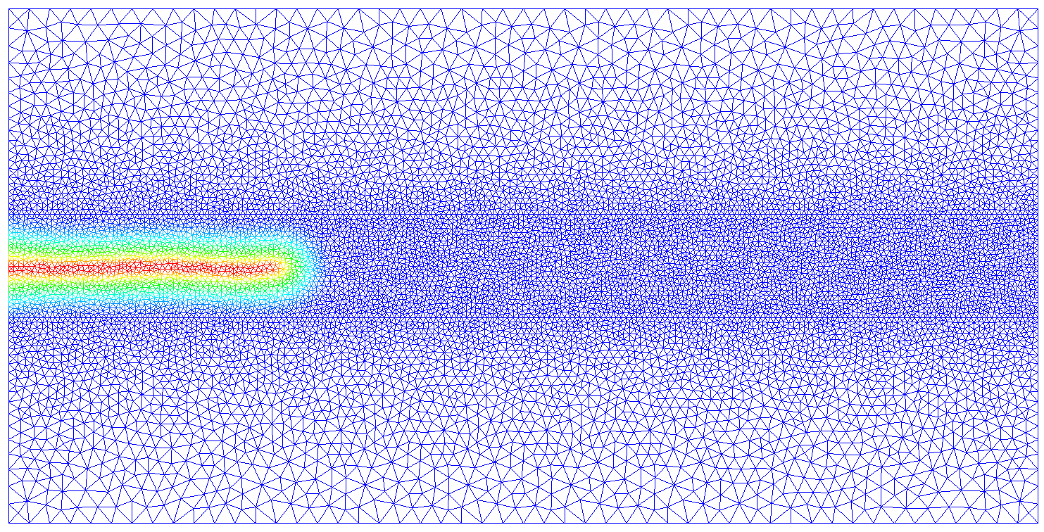
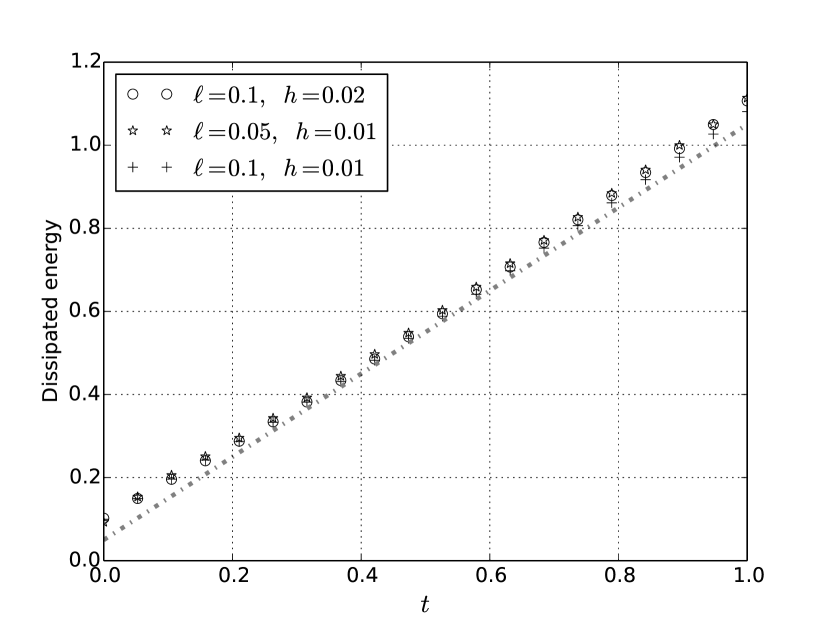
Figure 1: Smooth crack propagation test on a rectangular slab of dimensions $2\times 1$ with the surfing loading (24) applied on the boundary. Left: snapshot of the damage field and mesh for $\ell=0.05$ and $h=0.01$. Right: Dissipation energy versus time for $v=1$ and $K_{I}=1$ comparing the results obtained through the damage model when varying the internal length $\ell$ and the mesh size $h$; the continuous line is the expected surface energy according to the Griffith model, corresponding to a constant crack speed $v=1$. The given mesh size refers to the typical element dimension in the refined band in the middle.

4.2 Traction of a bar

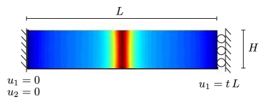
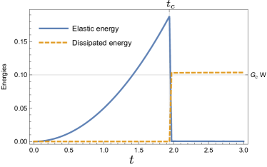
Figure 2: Uniaxial traction of bar. Left: boundary conditions and damage field for $t>t_{c}$. The width of the localization band may be calculated analytically and is given by $2\sqrt{2}\,\ell$. Right: evolution of the energy at the solution given by the minimization algorithm as the applied end-displacement $t$ is increased.

A basic problem of fracture mechanics is to estimate the ultimate load before fracture of a straight bar in traction. We consider a two dimensional bar of length $L$ and height $H$ under uniaxial traction with imposed displacement, as shown in figure 2. Analytical studies [30, 11] show that, for $L$ sufficiently greater that $\ell$, a local minimum of the energy functional (5) is the purely elastic solution $\alpha=0$ for $t<t_{c}=\sqrt{{3G_{c}}/{8E\ell}}$ and the solution with one crack represented in figure 2 for $t>t_{c}$. The cracked solution has a vanishing elastic energy and a surface energy given by $G_{c}\,W$. The test may be easily extended to a 3D geometry. The critical load $t_{c}$ is the same in 1D under a uniaxial stress condition, in 2D plane stress, or in 3D.

4.3 Thermal shock

The thermal shock problem of a brittle slab [32] is a challenging numerical test for the nucleation and propagation of multiple cracks. In physical experiments [68, 69], several ceramic slabs are bound together, uniformly heated to a high temperature and quenched in a cold bath, so as to submit the boundary of the domain to a thermal shock. The inhomogeneous temperature field induces an inhomogeneous stress field inside the slab, causing the emergence of a complex crack pattern, with an almost periodic array of cracks nucleating at the boundary and propagating inside the slab with a period doubling phenomenon. Following [32, 70], we consider a simplified model of this experimental test. The computational domain $\Omega=[-L/2,L/2]\times[0,H]$ (see Figure 3) is a slab of width $L$ and height $H$, with a thermal shock applied at the bottom surface $x_{2}=0$. At each timestep $\tau_{i}$, we seek the quasi-static evolution of the cracked state of the solid by solving for a stationary point of the following energy functional:

$${\mathcal{E}_{{\ell}}(u,\alpha)=\int_{\Omega}\dfrac{a(\alpha)}{2}A_{0}\,\varepsilon_{\mathrm{eff}}(u;\tau):\varepsilon_{\mathrm{eff}}(u;\tau)\ \mathrm{d}x}+\,{\dfrac{G_{c}}{c_{w}}\int_{\Omega}\left(\dfrac{w(\alpha)}{\ell}+\,{\ell}\,\nabla\alpha\cdot\nabla\alpha\right)\ \mathrm{d}x},$$ (25)

where $\varepsilon_{\mathrm{eff}}(u;\tau)=\varepsilon(u)-\varepsilon_{0}(\tau)$ is the effective elastic deformation accounting for the thermally induced inelastic strain

$$\varepsilon_{0}(\tau)={\beta\,T(\tau)\,I},\qquad T(\tau)=-\Delta T\,\mathrm{Erfc}\left(\dfrac{x_{2}/\ell}{\,\tau}\right),$$ (26)

where $\beta$ is the thermal expansion coefficient. The temperature field $T$ imposed is the analytical solution of an approximate thermal diffusion problem with a Dirichlet boundary condition on the temperature for a semi-infinite homogeneous slab of thermal diffusivity $k_{c}$. In particular, it neglects the influence of the cracks on the thermal diffusivity. The function $\mathrm{Erfc}$ denotes the complementary error function and $\tau=2\sqrt{{k}_{c}t/\ell^{2}}$ a dimensionless time acting as the loading parameter.

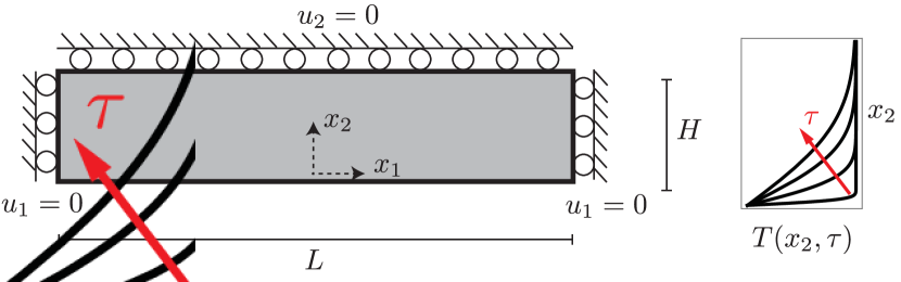
Figure 3: Geometry and boundary conditions for the thermal shock problem (left), where $u_{1}$ and $u_{2}$ denotes the two components of the displacement field. The loading is given by the thermal stress induced by the temperature field $T(x_{2},\tau)$ of (26), whose dependence in $x_{2}$ is sketched on the right for different times $\tau$.

As discussed in Bourdin et al. [32], the system is governed by three characteristic lengths: the size of the domain $L$, the internal length $\ell$, and the Griffith length $\ell_{0}={G_{c}}/{E(\beta\Delta T)^{2}}$. Hence, choosing $\ell$ as the reference length, the solution depends on two dimensionless parameters: the mildness of the thermal shock $\ell_{0}/\ell$ and the size of the slab $L/\ell$. Here we perform numerical simulations for fixed slab dimensions $L=20$ and internal length $\ell=1$. We apply the displacement boundary conditions described in Figure 3 and do not impose any Dirichlet boundary condition on the damage field. As can be show by dimensional analysis, without loss of generality, we set $E=1$, $G_{c}=1$, $\beta=1$. We consider the performance of the solver for varying $\Delta T$ and mesh sizes $h$.

Analytical and semi-analytical results are available for verification purposes and for the design of the numerical experiments. For $\Delta T<\Delta T_{c}=\sqrt{8E\ell/3\beta^{2}\,G_{c}}$ the solution is purely elastic with no damage ($\alpha=0$ everywhere) [32, 70]. For $\Delta T>\Delta T_{c}$ the solution evolves qualitatively as in Figure 4, with (i) the immediate creation of an $x$-homogeneous damage band parallel to the exposed surface, (ii) the bifurcation of this solution toward an $x$-periodic one, which (iii) further develops in a periodic array of crack bands orthogonal to the exposed surface. These bands further propagate with a period doubling phenomenon (iv). The three columns in Figure 4 show the phases (ii)-(iv) of the evolution for $\Delta T/\Delta T_{c}$ equal to 2, 4 and 8. The wavelength of the oscillations and the spacing of the cracks increase with $\Delta T$. In particular [32] shows that for $\Delta T\gg\Delta T_{c}$ the initial crack spacing is proportional to $\sqrt{\ell_{0}\ell}$. Figure 5 reports the evolution of the dissipated energy versus time for the three cases of Figure 4. We note in particular that, while the evolution is smooth for intense thermal shocks (see the curve $\Delta T=8\Delta T_{c}$), for mild shocks there are jumps in the energy dissipation and hence in the crack length (see the curve $\Delta T=2\Delta T_{c}$). These jumps correspond to snap-backs in the evolution problem, where the minimization algorithm is obliged to search for a new solution, potentially far from the one at the previous time step.

This problem constitutes a relevant and difficult test for the solver. First, the presence of a large number of cracks renders the elastic subproblem particularly ill-conditioned, and tests the effectiveness of the linear subsolvers and the coupled preconditioning strategy. Second, the presence of bifurcations and snap-backs stresses the convergence and effectiveness of the outer nonlinear solver. Third, the solution of the overall quasi-static evolution problem is strongly influenced by the irreversibility condition, testing the effectiveness of the variational inequality solvers.

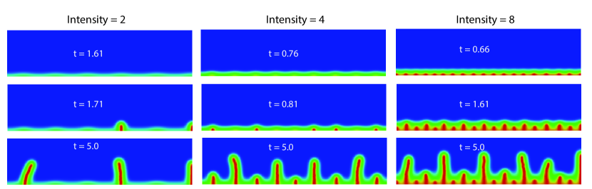
Figure 4: Snapshot of the evolution of the damage variable $\alpha$ during the evolution (blue: $\alpha=0$; red: $\alpha=1$) showing the initial solution independent of the $x_{1}$ variable, the emergence of a periodic crack pattern and its selective propagation with period doubling. Each column corresponds to the result obtained for a specific intensity, increasing from left (2) to right (8). Here $\ell=1$ and the slab dimensions are $40\times 10$ with a mesh size $h=0.2$.

Figure 5: Dissipated energy versus time for the thermal shock problem with intensity $\Delta T/\Delta T_{c}$ equal to 0.9, $2$, $4$ and $8$, as in Figure 4. For intensity $\Delta T=2\Delta T_{c}$, the evolution shows two clear jumps in time, corresponding to snapbacks and sudden crack growths. By contrast, the evolution is smooth for $\Delta T=8\Delta T_{c}$.

5 Results of numerical experiments

We present here the results of the numerical experiments that were performed to assess the performance of the proposed solvers. All problems were solved to an absolute $l_{2}$ residual tolerance of $10^{-7}$. For each test problem, we analyse the dependence of the results on the relevant physical parameter: we vary the internal length $\ell$ in the traction and surfing tests, and the intensity of the loading $\Delta T/\Delta T_{c}$ in the thermal shock problem.

5.1 Over-relaxation

We first consider ORAM, the over-relaxation of alternate minimization described in section 2.1. Each problem of section 4 was solved with values of the over-relaxation parameter $\omega$ taken from $\{0.8,1.0,\dots,1.8\}$. To consider the effect of over-relaxation alone, the Newton solver was disabled and all linear solves were performed with LU [71].

$\ell$	$\omega=0.8$	$\omega=1.0$	$\omega=1.2$	$\omega=1.4$	$\omega=1.6$	$\omega=1.8$	reduction
0.20	361	233	148	98	174	394	57.94%
0.10	564	369	251	159	148	307	59.89%
0.05	1168	773	537	368	236	320	69.47%
0.02	2523	1680	1182	835	569	461	72.56%

Table 1: Impact of over-relaxation on the surfing case. Standard alternate minimization converges slowly, and over-relaxation significantly reduces the number of iterations required.

$\ell$	$\omega=0.8$	$\omega=1.0$	$\omega=1.2$	$\omega=1.4$	$\omega=1.6$	$\omega=1.8$	reduction
0.10	124	53	111	181	324	729	0%
0.05	120	37	115	185	326	747	0%
0.02	132	39	121	195	332	726	0%
0.01	139	39	121	186	325	709	0%

Table 2: Impact of over-relaxation on the traction case. Standard alternate minimization converges rapidly for all values of $\ell$ and over-relaxation hinders convergence.

$\Delta T/\Delta T_{c}$	$\omega=0.8$	$\omega=1.0$	$\omega=1.2$	$\omega=1.4$	$\omega=1.6$	$\omega=1.8$	reduction
2	3577	2364	1685	1273	1095	1666	53.68%
4	3283	2156	1548	1184	1023	1611	52.55%
8	5100	2619	1844	1354	1094	1542	58.23%
16	5097	3382	2367	1669	1226	1756	63.75%

Table 3: Impact of over-relaxation on the thermal shock case. Standard alternate minimization converges slowly, and over-relaxation significantly reduces the number of iterations required.

The results for the surfing, traction and thermal shock problems are shown in Tables 3, 3 and 3 respectively. In all tables, the reduction column describes the decrease in iterations for the optimal $\omega$ compared to standard alternate minimization, $\omega=1$. In the traction case, standard alternate minimization is extremely efficient: a small number of iterations is required, the number of iterations required does not grow with $\ell$, and applying any other $\omega$ slows the convergence of the method. By contrast, in the surfing and thermal shock cases, standard alternate minimisation converges slowly, and the number of iterations required increases as the physical parameters $\ell$ and $\Delta T/\Delta T_{c}$ are varied. In this sense, the surfing and thermal shock cases are harder than the traction case. In these problems, over-relaxation helps significantly, reducing the number of iterations required by a factor between $1/2$ and $3/4$. Furthermore, the advantage gained by over-relaxation increases as the problem gets harder.

5.2 Composition of alternate minimization with Newton’s method

We next consider ORAM-N, the composition of alternate minimization with Newton’s method as described in section 2.3. For these experiments, Newton’s method was attempted once alternate minimization had reduced the $l_{2}$ norm of the residual by $10^{-1}$. All linear solves (both for alternate minimization and Newton’s method) were performed with LU, and all alternate minimizations employed the optimal over-relaxation parameter determined in the previous experiments ($\omega=1.6$ for the surfing and thermal shock cases, $\omega=1$ for the traction case). The time in seconds was measured for both approaches, as comparing iteration counts would be irrelevant. The runs were executed in serial on an otherwise unloaded Intel Xeon E5-4627 3.30 GHz CPU with 512 GB of RAM.

	time (s)
$\ell$	alternate minimization alone	composite solver	reduction
0.20	9.11	3.68	59.60%
0.10	27.00	15.43	42.85%
0.05	168.42	96.83	42.51%
0.02	2643.86	1886.53	28.64%

Table 4: Combining alternate minimization with Newton’s method for the surfing case. This further reduces the runtime of the solver compared to over-relaxed alternate minimization.

	time (s)
$\ell$	alternate minimization alone	composite solver	reduction
0.10	2.94	2.60	11.56%
0.05	5.94	5.71	3.87%
0.02	41.90	29.32	30.02%
0.01	195.97	175.06	10.67%

Table 5: Combining alternate minimization with Newton’s method for the traction case. In this case, the gains are modest.

	time (s)
$\Delta T/\Delta T_{c}$	alternate minimization alone	composite solver	reduction
2	312.29	215.68	30.94%
4	319.87	220.73	30.99%
8	335.38	238.28	28.95%
16	386.57	287.48	25.63%

Table 6: Combining alternate minimization with Newton’s method for the thermal shock case. This further reduces the runtime of the solver compared to over-relaxed alternate minimization.

The results for the surfing, traction and thermal shock problems are shown in Tables 6, 6 and 6 respectively. Again, the traction case is unusual compared to the other two: while the gains are marginal in the traction case, composition yields a worthwhile and consistent reduction in runtime for the other tests. If a more robust semismooth Newton solver were available, the speedup from composition would further increase.

5.3 Preconditioning the full Jacobian

The preconditioner (20) requires inner solvers for the displacement elasticity operator $A$ and the damage Helmholtz operator $C$. We first consider the performance of (20) with ideal inner solvers (LU), to investigate how the iteration counts scale with the physical parameters and with mesh size $h$. We then consider the performance with practical inner solvers, two V-cycles of algebraic multigrid for $A$ and $C$. Each Jacobian solve was terminated when the $l_{2}$ norm of the residual was reduced by a factor of $10^{-6}$, although adaptive tolerance selection should be used in practical calculations to retain quadratic convergence of the inexact Newton method [72]. For each configuration of physical parameters and $h$, the total number of Krylov iterations required for convergence over all loading steps was divided by the total number of Newton iterations, to compute the average number of Krylov iterations required to solve a Jacobian. In these experiments the alternate minimization was terminated with a relative residual reduction of $10^{-3}$, or if the absolute residual norm reached $10^{-6}$. As the gains from employing Newton’s method in the traction case were marginal, we consider here only the surfing and thermal shock problems.

	average Krylov iterations
$\ell$	$h=\ell/5$	$h=\ell/10$	$h=\ell/15$
0.20	6.17	9.47	12.03
0.10	8.92	10.91	13.53
0.05	10.74	13.07	15.58
0.02	13.07	14.95	18.03

Table 7: The average Krylov iterations per Newton step for different internal lengths $\ell$ and mesh sizes $h$ for the surfing case, with ideal inner solvers (LU). The preconditioner depends weakly on mesh refinement and on $\ell$.

	average Krylov iterations
$\ell$	$h=\ell/5$	$h=\ell/10$	$h=\ell/15$
0.20	6.33	10.57	11.64
0.10	8.50	10.93	13.68
0.05	11.13	13.53	16.15
0.02	13.53	15.61	18.80

Table 8: The average Krylov iterations per Newton step for different internal lengths $\ell$ and mesh sizes $h$ for the surfing case, with practical inner solvers (AMG). Switching to practical inner solvers hardly affects the convergence of the preconditioner.

	average Krylov iterations
$\Delta T/\Delta T_{c}$	$h=\ell/4$	$h=\ell/8$	$h=\ell/16$
2	10.11	7.87	6.87
4	10.56	11.44	14.70
8	15.97	19.64	17.75
16	23.15	22.37	22.03

Table 9: The average Krylov iterations per Newton step for different intensities $\Delta T/\Delta T_{c}$ and mesh sizes $h$ for the thermal shock case, with ideal inner solvers (LU). The preconditioner depends weakly on mesh refinement and on Griffith length.

	average Krylov iterations
$\Delta T/\Delta T_{c}$	$h=\ell/4$	$h=\ell/8$	$h=\ell/16$
2	15.25	12.54	11.82
4	12.95	13.42	18.25
8	19.08	19.65	22.51
16	27.79	27.22	29.54

Table 10: The average Krylov iterations per Newton step for different intensities $\Delta T/\Delta T_{c}$ and mesh sizes $h$ for the thermal shock case, with practical inner solvers (AMG). In this case, using practical inner solvers somewhat degrades the convergence of the preconditioner.

The results for the surfing case with ideal and practical inner solvers are shown in Tables 10 and 10, and the corresponding results for the thermal shock case are shown in Tables 10 and 10. In the surfing case, the number of iterations required grows slowly as the mesh is refined, and grows slowly as $\ell$ is reduced. However, even for the smallest $\ell$ on the finest mesh, the number of outer Krylov iterations required is modest, and the results barely differ if the ideal inner solvers are replaced with practical variants. In the thermal shock case, the number of iterations required stays approximately constant as the mesh is refined, and grows slowly with the intensity $\Delta T/\Delta T_{c}$. Here, replacing the ideal inner solvers with practical variants does have a measurable cost in iteration count; this could be reduced by tuning the parameters of the algebraic multigrid algorithm employed, or by employing stronger inner solvers. These results show that the preconditioner (20) is a practical and efficient solver for the full coupled Jacobian, whose performance degrades slowly as the difficulty of the problem is increased.

6 Conclusion

In this paper we proposed several improvements to the current standard algorithm for solving variational fracture models. Over-relaxation is extremely cheap and simple to implement, but can greatly reduce the number of iterations required for convergence. Composing over-relaxed alternate minimization with Newton-type methods yields a further decrease in runtime, although at a more significant development cost. Together, these improvements to alternate minimization reduce the time to solution by a factor of 5–6$\times$ for the surfing and thermal shock test cases. Lastly, we proposed and tested preconditioners for the linear subproblems in alternate minimization and the coupled Jacobian arising in the Newton iterations when solving the whole problem with a monolithic active set method. These efforts are complementary to other approaches recently proposed in the literature, such as adaptive remeshing [44], adaptive time-stepping, continuation algorithms [39], or refined line-search techniques [40] that were not considered in this work. Our tests focus only on the simplest settings for variational fracture mechanics assuming small deformations and a simple rate-independent material behaviour. However, the developed techniques can be readily adapted to more complex contexts, including hyperelasticity, viscoelasticity, and inertial effects.

These results suggest several directions for future research. It would be highly desirable to develop a convergence analysis of block over-relaxed nonlinear Gauss-Seidel for variational inequalities, although we do not anticipate this will yield constructive insight for the choice of the over-relaxation parameter $\omega$. It may be possible to design $\ell$-robust preconditioners for the coupled Jacobian (where the convergence is independent of $\ell$) by choosing appropriate $\ell$-dependent inner products for the displacement and damage function spaces. If the appropriate Babuška constants are independent of $\ell$, the convergence will be also [73].

In this work we have considered only the simplest fracture model, assuming small deformations and symmetric behaviour in traction and compression. Our developments on over-relaxation and composition of alternate minimization with Newton could be applied with minor modifications to more complex cases, including for example the tension-compression splitting of the elastic energy to account for the non-interpenetration condition on the crack lips [22, 23, 24, 25, 26]. In this case an efficient solver would require the development of suitable preconditioners for the elastic subproblem and the coupled Jacobian.

References

- [1] Francfort G, Marigo JJ. Revisiting brittle fracture as an energy minimization problem. Journal of the Mechanics and Physics of Solids 1998; 46(8):1319–1342.
- [2] Griffith A. The phenomena of rupture and flow in solids. Philosophical Transactions of the Royal Society A 1921; 221:163–198.
- [3] Francfort G, Bourdin B, Marigo JJ. The variational approach to fracture. Journal of Elasticity 2008; 91(1-3):5–148.
- [4] Ambrosio L, Fusco N, Pallara D. Functions of Bounded Variations and Free Discontinuity Problems. Oxford Mathematical Monographs, Oxford Science Publications, 2000.
- [5] Bourdin B, Francfort GA, Marigo JJ. Numerical experiments in revisited brittle fracture. Journal of the Mechanics and Physics of Solids 2000; 48:787–826.
- [6] Ambrosio L, Tortorelli VM. On the approximation of free discontinuity problems. Bollettino dell’Unione Matematica Italiana 1992; 7(6-B):105–123.
- [7] Mumford D, Shah J. Optimal approximations by piecewise smooth functions and associated variational problems. Communications on Pure and Applied Mathematics 1989; 42:577–685.
- [8] Giacomini A. Ambrosio-Tortorelli approximation of quasi-static evolution of brittle fractures. Calculus of Variations and Partial Differential Equations 2005; 22:129–172.
- [9] Hakim V, Karma A. Laws of crack motion and phase-field models of fracture. Journal of the Mechanics and Physics of Solids 2009; 57(2):342–368.
- [10] Lorentz E, Godard V. Gradient damage models: toward full-scale computations. Computer Methods in Applied Mechanics and Engineering 2011; 200(21–22):1927–1944.
- [11] Pham K, Amor H, Marigo JJ, Maurini C. Gradient damage models and their use to approximate brittle fracture. International Journal of Damage Mechanics 2011; 20(4):618–652.
- [12] Bourdin B, Larsen C, Richardson C. A time-discrete model for dynamic fracture based on crack regularization. International Journal of Fracture 2011; 168(2):133–143.
- [13] Borden MJ, Verhoosel CV, Scott MA, Hughes TJ, Landis CM. A phase-field description of dynamic brittle fracture. Computer Methods in Applied Mechanics and Engineering 2012; 217–220(0):77–95.
- [14] Schlüter A, Willenbücher A, Kuhn C, Müller R. Phase field approximation of dynamic brittle fracture. Computational Mechanics 2014; 54(5):1–21.
- [15] Abdollahi A, Arias I. Phase-field modeling of crack propagation in piezoelectric and ferroelectric materials with different electromechanical crack conditions. Journal of the Mechanics and Physics of Solids 2012; 60(12):2100–2126.
- [16] Wheeler MF, Wick T, Wollner W. An augmented-Lagrangian method for the phase-field approach for pressurized fractures. Computer Methods in Applied Mechanics and Engineering 4 2014; 271(0):69–85.
- [17] Li B, Peco C, Millán D, Arias I, Arroyo M. Phase-field modeling and simulation of fracture in brittle materials with strongly anisotropic surface energy. International Journal for Numerical Methods in Engineering 2014; 102(3–4):711–727.
- [18] Del Piero G, Lancioni G, March R. A variational model for fracture mechanics: numerical experiments. Journal of the Mechanics and Physics of Solids 2007; 55:2513–2537.
- [19] Clayton J, Knap J. A geometrically nonlinear phase field theory of brittle fracture. International Journal of Fracture 2014; 189(2):1–10.
- [20] Hesch C, Weinberg K. Thermodynamically consistent algorithms for a finite-deformation phase-field approach to fracture. International Journal for Numerical Methods in Engineering 2014; 99(12):906–924.
- [21] Verhoosel CV, de Borst R. A phase-field model for cohesive fracture. International Journal for Numerical Methods in Engineering 2013; 96(1):43–62.
- [22] Amor H, Marigo JJ, Maurini C. Regularized formulation of the variational brittle fracture with unilateral contact: Numerical experiments. Journal of the Mechanics and Physics of Solids 2009; 57(8):1209–1229.
- [23] Lancioni G, Royer-Carfagni G. The variational approach to fracture mechanics. A practical application to the French Panthéon in Paris. Journal of Elasticity 2009; 95:1–30.
- [24] Freddi F, Royer-Carfagni G. Regularized variational theories of fracture: a unified approach. Journal of the Mechanics and Physics of Solids 2010; 58:1154–1174.
- [25] Miehe C, Welschinger F, Hofacker M. Thermodynamically consistent phase-field models of fracture: Variational principles and multi-field FE implementations. International Journal for Numerical Methods in Engineering 2010; 83(10):1273–1311.
- [26] Ambati M, Gerasimov T, De Lorenzis L. A review on phase-field models of brittle fracture and a new fast hybrid formulation. Computational Mechanics 2015; 55(2):383–405.
- [27] Amiri F, Millán D, Shen Y, Rabczuk T, Arroyo M. Phase-field modeling of fracture in linear thin shells. Theoretical and Applied Fracture Mechanics 2014; 69:102 – 109.
- [28] Ambati M, Lorenzis LD. Phase-field modeling of brittle and ductile fracture in shells with isogeometric nurbs-based solid-shell elements. Computer Methods in Applied Mechanics and Engineering 2016; :–.
- [29] Leon Baldelli A, Babadjian JF, Bourdin B, Henao D, Maurini C. A variational model for fracture and debonding of thin films under in-plane loadings. Journal of the Mechanics and Physics of Solids 2014; 70(0):320–348.
- [30] Pham K, Marigo JJ, Maurini C. The issues of the uniqueness and the stability of the homogeneous response in uniaxial tests with gradient damage models. Journal of the Mechanics and Physics of Solids 2011; 59(6):1163–1190.
- [31] Pham K, Marigo JJ. From the onset of damage to rupture: Construction of responses with damage localization for a general class of gradient damage models. Continuum Mechanics and Thermodynamics 2013; 25(2-4):147–171. Cited By (since 1996)1.
- [32] Bourdin B, Marigo JJ, Maurini C, Sicsic P. Morphogenesis and propagation of complex cracks induced by thermal shocks. Physical Review Letters 2014; 112:014 301.
- [33] Bourdin B. Numerical implementation of the variational formulation for quasi-static brittle fracture. Interfaces and Free Boundaries 2007; 9:411—430.
- [34] Miehe C, Hofacker M, Welschinger F. A phase field model for rate-independent crack propagation: Robust algorithmic implementation based on operator splits. Computer Methods in Applied Mechanics and Engineering 2010; 199(45–48):2765–2778.
- [35] Facchinei F, Júdice J, Soares J. An active set Newton algorithm for large-scale nonlinear programs with box constraints. SIAM Journal on Optimization 1998; 8(1):158–186.
- [36] Ulbrich M. Semismooth Newton Methods for Variational Inequalities and Constrained Optimization Problems in Function Spaces, MOS-SIAM Series on Optimization, vol. 11. SIAM, 2011.
- [37] Lorentz E, Badel P. A new path-following constraint for strain-softening finite element simulations. International Journal for Numerical Methods in Engineering 2004; 60(2):499–526.
- [38] Heister T, Wheeler MF, Wick T. A primal-dual active set method and predictor-corrector mesh adaptivity for computing fracture propagation using a phase-field approach. Computer Methods in Applied Mechanics and Engineering 2015; 290:466–495.
- [39] Singh N, Verhoosel C, de Borst R, van Brummelen E. A fracture-controlled path-following technique for phase-field modeling of brittle fracture. Finite Elements in Analysis and Design 2016; 113:14 – 29.
- [40] Gerasimov T, De Lorenzis L. A line search assisted monolithic approach for phase-field computing of brittle fracture. Computer Methods in Applied Mechanics and Engineering in press; :–http://dx.doi.org/10.1016/j.cma.2015.12.017. URL http://www.sciencedirect.com/science/article/pii/S0045782515004235.
- [41] Negri M. The anisotropy introduced by the mesh in the finite element approximation of the Mumford-Shah functional. Numerical Functional Analysis and Optimization 1999; 20:957–982.
- [42] Bellettini G, Coscia A. Discrete approximation of a free discontinuity problem. Numerical Functional Analysis and Optimization 1994; 15:105–123.
- [43] Burke S, Ortner C, Süli E. An adaptive finite element approximation of a variational model of brittle fracture. SIAM Journal on Numerical Analysis 2010; 48(3):980–1012.
- [44] Artina M, Fornasier M, Micheletti S, Perotto S. Anisotropic mesh adaptation for crack detection in brittle materials. SIAM Journal on Scientific Computing 2015; 37(4):B633–B659.
- [45] Brune P, Knepley MG, Smith B, Tu X. Composing scalable nonlinear algebraic solvers. preprint ANL/MCS-P2010-0112, Argonne National Laboratory 2013.
- [46] Ortega J, Rheinboldt W. Iterative Solution of Nonlinear Equations in Several Variables. SIAM, 2000.
- [47] Young DM. Iterative methods for solving partial difference equations of elliptic type. PhD Thesis, Harvard University, Massachusetts, USA 1950.
- [48] Arms RJ, Gates LD, Zondek B. A method of block iteration. Journal of the Society for Industrial and Applied Mathematics 1956; 4(4):220–229.
- [49] Kahan W. Gauss-Seidel methods of solving large systems of linear equations. PhD Thesis, University of Toronto, Ontario, Canada 1958.
- [50] Ostrowski AM. On the linear iteration procedures for symmetric matrices. Rendiconti di Matematica e sue Applicazioni 1954; 5(14):140–163.
- [51] Reid JK. A method for finding the optimum successive over-relaxation parameter. The Computer Journal 1966; 9(2):200–204, 10.1093/comjnl/9.2.200.
- [52] Munson TS. Algorithms and environments for complementarity. PhD Thesis, University of Wisconsin-Madison, Wisconsin, USA 2000.
- [53] Benson SJ, Munson TS. Flexible complementarity solvers for large-scale applications. Optimization Methods and Software 2006; 21(1):155–168.
- [54] Fischer A. A special Newton-type optimization method. Optimization 1992; 24(3–4):269–284.
- [55] Facchinei F, Soares J. A new merit function for nonlinear complementarity problems and a related algorithm. SIAM Journal on Optimization 1997; 7(1):225–247.
- [56] Hestenes MR, Stiefel E. Methods of conjugate gradients for solving linear systems. Journal of Research of the National Bureau of Standards 1952; 49(6):409–436.
- [57] Adams MF, Bayraktar HH, Keaveny TM, Papadopoulos P. Ultrascalable implicit finite element analyses in solid mechanics with over a half a billion degrees of freedom. ACM/IEEE Proceedings of SC2004: High Performance Networking and Computing, Pittsburgh, Pennsylvania, 2004.
- [58] Falgout RD. An introduction to algebraic multigrid computing. Computing in Science & Engineering 2006; 8(6):24–33.
- [59] Hernandez V, Roman JE, Vidal V. SLEPc: A scalable and flexible toolkit for the solution of eigenvalue problems. ACM Transactions on Mathematical Software 2005; 31(3):351–362.
- [60] Vaněk P, Mandel J, Brezina M. Algebraic multigrid by smoothed aggregation for second and fourth order elliptic problems. Computing 1996; 56(3):179–196.
- [61] Gee M, Siefert C, Hu J, Tuminaro R, Sala M. ML 5.0 smoothed aggregation user’s guide. Technical Report SAND2006-2649, Sandia National Laboratories 2006.
- [62] Murphy MF, Golub GH, Wathen AJ. A note on preconditioning for indefinite linear systems. SIAM Journal on Scientific Computing 2000; 21(6):1969–1972.
- [63] Benzi M, Golub GH, Liesen J. Numerical solution of saddle point problems. Acta Numerica 5 2005; 14:1–137.
- [64] Brown J, Knepley M, May D, McInnes L, Smith B. Composable linear solvers for multiphysics. 2012 11th International Symposium on Parallel and Distributed Computing (ISPDC), 2012; 55–62.
- [65] Balay S, Abhyankar S, Adams MF, Brown J, Brune P, Buschelman K, Eijkhout V, Gropp WD, Kaushik D, Knepley MG, et al.. PETSc users manual. Technical Report ANL-95/11 - Revision 3.5, Argonne National Laboratory 2014.
- [66] Paige C, Saunders M. Solution of sparse indefinite systems of linear equations. SIAM Journal on Numerical Analysis 1975; 12(4):617–629.
- [67] Hossain M, Hsueh CJ, Bourdin B, Bhattacharya K. Effective toughness of heterogeneous media. Journal of the Mechanics and Physics of Solids 2014; 71(0):15–32.
- [68] Bahr HA, Weiss HJ, Maschke H, Meissner F. Multiple crack propagation in a strip caused by thermal shock. Theoretical and Applied Fracture Mechanics 1988; 10:219–226.
- [69] Jiang C, Wu X, Li J, Song F, Shao Y, Xu X, Yan P. A study of the mechanism of formation and numerical simulations of crack patterns in ceramics subjected to thermal shock. Acta Materialia 2012; 60(11):4540–4550.
- [70] Sicsic P, Marigo JJ, Maurini C. Initiation of a periodic array of cracks in the thermal shock problem: A gradient damage modeling. Journal of the Mechanics and Physics of Solids 2014; 63(0):256–284.
- [71] Amestoy PR, Duff IS, Koster J, L’Excellent JY. A fully asynchronous multifrontal solver using distributed dynamic scheduling. SIAM Journal on Matrix Analysis and Applications 2001; 23(1):15–41.
- [72] Eisenstat S, Walker H. Choosing the forcing terms in an inexact Newton method. SIAM Journal on Scientific Computing 1996; 17(1):16–32.
- [73] Mardal KA, Winther R. Preconditioning discretizations of systems of partial differential equations. Numerical Linear Algebra with Applications 2011; 18(1):1–40.