Generalized deviation equation and determination of the curvature in General Relativity

Abstract

We derive a generalized deviation equation – analogous to the well-known geodesic deviation equation – for test bodies in General Relativity. Our result encompasses and generalizes previous extensions of the standard geodesic deviation equation. We show how the standard as well as a generalized deviation equation can be used to measure the curvature of spacetime by means of a set of test bodies. In particular, we provide exact solutions for the curvature by using the standard deviation equation as well as its next order generalization.

I Introduction

In General Relativity, the comparison of test bodies moving along adjacent world lines is of direct operational significance. The observation of a suitably prepared set of test bodies allows for the determination of the components of the curvature tensor. In this work we derive a deviation equation for test bodies moving along general curves in arbitrary background spacetimes.

Our findings in this work generalize the well-known geodesic deviation equation and some of its early modifications. In contrast to many previous treatments, we are making use of a covariant expansion technique based on Synge’s “world function” Synge (1960); DeWitt and Brehme (1960). This expansion technique has also been applied extensively in the context of the equations of motion of extended test bodies Dixon (1964, 1974, 1979, 2008); Puetzfeld and Obukhov (2014); Dixon (2015); Obukhov and Puetzfeld (2015) and in the gravitational self-force problem Ottewill and Wardell (2011); Poisson et al. (2011).

We explicitly show, how the deviation equation can be used to measure the curvature of spacetime and thereby the gravitational field. For this we extend Szekeres’ “gravitational compass” Szekeres (1965) and provide an exact solution for the curvature components in terms of the mutual accelerations between the constituents of a swarm of test bodies.

The structure of the paper is as follows: In section II we derive an exact generalized deviation along general world lines. Furthermore, we provide a systematic expansion of this equation in powers of the deviation vector. Subsequently we study several special cases of our general deviation equation in section III. In particular, we make contact with several other suggestions for deviation equations in the literature. We then use the derived deviation equation in section IV to determine the curvature of spacetime by means of a generalized gravitational compass. We conclude our paper in section V with a discussion of the results obtained and with an outlook of their possible applications. Our notations and conventions are summarized in appendix A and table 2. An exposition on normal coordinates given in appendix B contains some new results not found in the earlier literature.

II Generalized deviation equation

Alternative derivations and generalizations Plebański (1965); Hodgkinson (1972); Bażański (1974); Hojman (1975); Bażański (1976, 1977a, 1977b); Novello et al. (1977); Aleksandrov and Piragas (1978); Manoff (1979); Schattner and Trümper (1981); Swaminarayan and Safko (1983); Schutz (1985); Kamran and Marck (1986); Ciufolini (1986); Bażański and Kostyukovich (1987a, b); Bażański (1989); Vanzo (1992); Roberts (1996); Kerner et al. (2001); Manoff (2001); van Holten (2002); Chicone and Mashhoon (2002); Nieto et al. (2003); Mohseni (2004); Heydari-Fard et al. (2005); Perlick (2008); Vines (2015) as well as applications Szekeres (1965); Shirokov (1973); Greenberg (1974); Mashhoon (1975, 1977); Tammelo (1977); Dolan et al. (1980); Caviglia et al. (1982); Fuchs (1983); Audretsch and Lämmerzahl (1983); Tammelo (1984); Bażański (1986); Ciufolini and Demianski (1986); Bażański and Kostyukovich (1987c); Bażański and Jaranowski (1989); Fuchs (1990a, b); Mohseni and Sepangi (2000); Balakin et al. (2000); Colistete et al. (2002); Biesiada (2003); Baskaran and Grishchuk (2004); Mullari and Tammelo (2006); Mortazavimanesh and Mohseni (2009); Bini et al. (2011); Koekoek and van Holten (2011) of the standard and generalized deviation equations have been extensively studied in the physical and mathematical literature. The interest in deviation equations is of course directly linked to their operational meaning, allowing for a measurement of the gravitational field, i.e. the curvature of spacetime, in General Relativity.

Here we focus on a covariant derivation of a deviation equation for general curves, which are not necessarily geodesic. We base our derivation on Synge’s world function $\sigma(x,y)$ Synge (1960), which introduces a covariant generalization of the finite distance between the spacetime points $x$ and $y$. Basic definitions and our notation are summarized in appendix A.

II.1 Comparison of two general curves

Let us start by comparing two general curves $Y(t)$ and $X(\tilde{t})$ in an arbitrary spacetime manifold. At this stage even the parameters $t$ and $\tilde{t}$ can be general, i.e. are not necessarily the proper time on the given curves. Now we connect two points $x\in X$ and $y\in Y$ on the two curves by the geodesic joining the two points (we assume that this geodesic is unique).

Along the geodesic we have the world function $\sigma$, and conceptually the closest object to the connecting vector between the two points is the covariant derivative of the world function, denoted at the point $y$ by $\sigma^{y}$. Note though that $\sigma^{y}$ is just tangent at that point (its length being the the geodesic length between $y$ and $x$), only in flat spacetime it coincides with the connecting vector. Keeping in mind such an interpretation, let us now work out a propagation equation for this “generalized” connecting vector along the reference curve, cf. fig. 1. Following our conventions the reference curve will be $Y(t)$ and we define the generalized connecting vector to be:

$$\eta^{y}:=-\sigma^{y}$$ (1)

Taking its covariant total derivative, we have

$$\frac{D}{dt}\eta^{y_{1}} = -\frac{D}{dt}\sigma^{y_{1}}\left(Y(t),X(\tilde{t})\right)$$ (2)

$$= -\sigma^{y_{1}}{}_{y_{2}}\frac{\partial Y^{y_{2}}}{\partial t}-\sigma^{y_{1}}{}_{x_{2}}\frac{\partial X^{x_{2}}}{\partial\tilde{t}}\frac{d\tilde{t}}{dt}$$

$$= -\sigma^{y_{1}}{}_{y_{2}}u^{y_{2}}-\sigma^{y_{1}}{}_{x_{2}}\tilde{u}^{x_{2}}\frac{d\tilde{t}}{dt},$$

where in the last line we defined the velocities along the two curves $Y$ and $X$. As usual, $\sigma^{y}{}_{x_{1}\dots y_{2}\dots}:=\nabla_{x_{1}}\dots\nabla_{y_{2}}\dots(\sigma^{y})$ denote the higher order covariant derivatives of the world function. We continue by taking the second derivative of (2), which yields

$$\frac{D^{2}}{dt^{2}}\eta^{y_{1}} = -\sigma^{y_{1}}{}_{y_{2}y_{3}}u^{y_{2}}u^{y_{3}}-2\sigma^{y_{1}}{}_{y_{2}x_{3}}u^{y_{2}}\tilde{u}^{x_{3}}\frac{d\tilde{t}}{dt}$$ (3)

$$-\sigma^{y_{1}}{}_{y_{2}}a^{y_{2}}-\sigma^{y_{1}}{}_{x_{2}x_{3}}\tilde{u}^{x_{2}}\tilde{u}^{x_{3}}\left(\frac{d\tilde{t}}{dt}\right)^{2}$$

$$-\sigma^{y_{1}}{}_{x_{2}}\tilde{a}^{x_{2}}\left(\frac{d\tilde{t}}{dt}\right)^{2}-\sigma^{y_{1}}{}_{x_{2}}\tilde{u}^{x_{2}}\frac{d^{2}\tilde{t}}{dt^{2}},$$

here we introduced the accelerations $a^{y}:={Du^{y}}/dt$, and $\tilde{a}^{x}:={D\tilde{u}^{x}}/d\tilde{t}$. Equation (3) is already the generalized deviation equation, but the goal is to have all the quantities therein defined along the reference wordline $Y$.

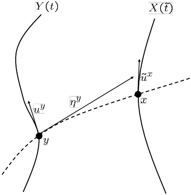
Figure 1: Sketch of the two arbitrarily parametrized world lines $Y(t)$ and $X(\tilde{t})$, and the geodesic connecting two points on these world line. The (generalized) deviation vector along the reference world line $Y$ is denoted by $\eta^{y}$.

We now derive some auxiliary formulas, by introducing the inverse of the second derivative of the world function via the following equations:

$$\stackrel{{\scriptstyle-1}}{{\sigma}}\!\!{}^{y_{1}}{}_{x}\sigma^{x}{}_{y_{2}} = \delta^{y_{1}}{}_{y_{2}},$$ (4)

$$\stackrel{{\scriptstyle-1}}{{\sigma}}\!\!{}^{x_{1}}{}_{y}\sigma^{y}{}_{x_{2}} = \delta^{x_{1}}{}_{x_{2}}.$$ (5)

Multiplication of (2) by $\stackrel{{\scriptstyle-1}}{{\sigma}}\!\!{}^{x_{3}}{}_{y_{1}}$ then yields

$$\tilde{u}^{x_{3}}\frac{d\tilde{t}}{dt} = -\stackrel{{\scriptstyle-1}}{{\sigma}}\!\!{}^{x_{3}}{}_{y_{1}}\sigma^{y_{1}}{}_{y_{2}}u^{y_{2}}+\stackrel{{\scriptstyle-1}}{{\sigma}}\!\!{}^{x_{3}}{}_{y_{1}}\frac{D\sigma^{y_{1}}}{dt}$$ (6)

$$= K^{x_{3}}{}_{y_{2}}u^{y_{2}}-H^{x_{3}}{}_{y_{1}}\frac{D\sigma^{y_{1}}}{dt}.$$

Where in the last line we defined two auxiliary quantities $K^{x}{}_{y}$ and $H^{x}{}_{y}$ – the notation follows the terminology of Dixon. Equation (6) allows us to formally express the the velocity along the curve $X$ in terms of the quantities which are defined at $Y$ and then “propagated” by $K^{x}{}_{y}$ and $H^{x}{}_{y}$. Using (6) in (3) we arrive at:

$$\frac{D^{2}}{dt^{2}}\eta^{y_{1}} = -\sigma^{y_{1}}{}_{y_{2}y_{3}}u^{y_{2}}u^{y_{3}}-\sigma^{y_{1}}{}_{y_{2}}a^{y_{2}}$$ (7)

$$-2\sigma^{y_{1}}{}_{y_{2}x_{3}}u^{y_{2}}\left(K^{x_{3}}{}_{y_{4}}u^{y_{4}}-H^{x_{3}}{}_{y_{4}}\frac{D\sigma^{y_{4}}}{dt}\right)$$

$$-\sigma^{y_{1}}{}_{x_{2}x_{3}}\left(K^{x_{2}}{}_{y_{4}}u^{y_{4}}-H^{x_{2}}{}_{y_{4}}\frac{D\sigma^{y_{4}}}{dt}\right)$$

$$\times\left(K^{x_{3}}{}_{y_{5}}u^{y_{5}}-H^{x_{3}}{}_{y_{5}}\frac{D\sigma^{y_{5}}}{dt}\right)$$

$$-\sigma^{y_{1}}{}_{x_{2}}\frac{D}{dt}\left(K^{x_{2}}{}_{y_{3}}u^{y_{3}}-H^{x_{2}}{}_{y_{3}}\frac{D\sigma^{y_{3}}}{dt}\right).$$

We may derive an alternative version of this equation – by using (6) multiplied by $dt/d\tilde{t}$ – which yields

$$\tilde{u}^{x_{3}} = K^{x_{3}}{}_{y_{2}}u^{y_{2}}\frac{dt}{d\tilde{t}}-H^{x_{3}}{}_{y_{1}}\frac{D\sigma^{y_{1}}}{dt}\frac{dt}{d\tilde{t}},$$ (8)

and inserted into (3):

$$\frac{D^{2}}{dt^{2}}\eta^{y_{1}} = -\sigma^{y_{1}}{}_{y_{2}y_{3}}u^{y_{2}}u^{y_{3}}-\sigma^{y_{1}}{}_{y_{2}}a^{y_{2}}-\sigma^{y_{1}}{}_{x_{2}}\tilde{a}^{x_{2}}\left(\frac{d\tilde{t}}{dt}\right)^{2}$$ (9)

$$-2\sigma^{y_{1}}{}_{y_{2}x_{3}}u^{y_{2}}\left(K^{x_{3}}{}_{y_{4}}u^{y_{4}}-H^{x_{3}}{}_{y_{4}}\frac{D\sigma^{y_{4}}}{dt}\right)$$

$$-\sigma^{y_{1}}{}_{x_{2}x_{3}}\left(K^{x_{2}}{}_{y_{4}}u^{y_{4}}-H^{x_{2}}{}_{y_{4}}\frac{D\sigma^{y_{4}}}{dt}\right)$$

$$\times\left(K^{x_{3}}{}_{y_{5}}u^{y_{5}}-H^{x_{3}}{}_{y_{5}}\frac{D\sigma^{y_{5}}}{dt}\right)$$

$$-\sigma^{y_{1}}{}_{x_{2}}\frac{dt}{d\tilde{t}}\frac{d^{2}\tilde{t}}{dt^{2}}\left(K^{x_{2}}{}_{y_{3}}u^{y_{3}}-H^{x_{2}}{}_{y_{3}}\frac{D\sigma^{y_{3}}}{dt}\right).$$

Note that we may determine the factor $d\tilde{t}/dt$ by requiring that the velocity along the curve $X$ is normalized, i.e. $\tilde{u}^{x}\tilde{u}_{x}=1$, in which case (6) yields

$$\frac{d\tilde{t}}{dt} = \tilde{u}_{x_{1}}K^{x_{1}}{}_{y_{2}}u^{y_{2}}-\tilde{u}_{x_{1}}H^{x_{1}}{}_{y_{2}}\frac{D\sigma^{y_{2}}}{dt}.$$ (10)

II.2 Expansion of quantities on $Y$

The generalized (exact) deviation equations (7) and (9) contain quantities which are not defined along the reference curve, in particular the covariant derivatives of the world function. We now make use of the covariant expansions of these quantities, which we already worked out in our previous paper Puetzfeld and Obukhov (2014), i.e.

$$\sigma^{y_{0}}{}_{x_{1}} = g^{y^{\prime}}{}_{x_{1}}\biggl{(}-\,\delta^{y_{0}}{}_{y^{\prime}}$$ (11)

$$+\,\sum\limits_{k=2}^{\infty}\,{\frac{1}{k!}}\,\alpha^{y_{0}}{}_{y^{\prime}y_{2}\!\dots\!y_{k+1}}\sigma^{y_{2}}\cdots\sigma^{y_{k+1}}\biggr{)}\!,$$

$$\sigma^{y_{0}}{}_{y_{1}} = \delta^{y_{0}}{}_{y_{1}}$$ (12)

$$-\,\sum\limits_{k=2}^{\infty}\,{\frac{1}{k!}}\,\beta^{y_{0}}{}_{y_{1}y_{2}\dots y_{k+1}}\sigma^{y_{2}}\!\cdots\!\sigma^{y_{k+1}},$$

$$g^{y_{0}}{}_{x_{1};x_{2}} = g^{y^{\prime}}{\!}_{x_{1}}g^{y^{\prime\prime}}{\!}_{x_{2}}\biggl{(}{\frac{1}{2}}R^{y_{0}}{}_{y^{\prime}y^{\prime\prime}y_{3}}\sigma^{y_{3}}$$ (13)

$$\!+\!\sum\limits_{k=2}^{\infty}\,{\frac{1}{k!}}\,\gamma^{y_{0}}{}_{y^{\prime}y^{\prime\prime}y_{3}\dots y_{k+2}}\sigma^{y_{3}}\!\cdots\!\sigma^{y_{k+2}}\!\biggr{)}\!,$$

$$g^{y_{0}}{}_{x_{1};y_{2}} = g^{y^{\prime}}{\!}_{x_{1}}\biggl{(}{\frac{1}{2}}R^{y_{0}}{}_{y^{\prime}y_{2}y_{3}}\sigma^{y_{3}}$$ (14)

$$\!+\!\sum\limits_{k=2}^{\infty}\,{\frac{1}{k!}}\,\gamma^{y_{0}}{}_{y^{\prime}y_{2}y_{3}\dots y_{k+2}}\sigma^{y_{3}}\!\cdots\!\sigma^{y_{k+2}}\!\biggr{)}.$$

The coefficients $\alpha,\beta,\gamma$ in these expansions are polynomials constructed from the Riemann curvature tensor and its covariant derivatives. The first coefficients read (as one can also check using computer algebra Ottewill and Wardell (2011)):

$$\alpha^{y_{0}}{}_{y_{1}y_{2}y_{3}} = -\,\frac{1}{3}R^{y_{0}}{}_{(y_{2}y_{3})y_{1}},$$ (15)

$$\beta^{y_{0}}{}_{y_{1}y_{2}y_{3}} = \frac{2}{3}R^{y_{0}}{}_{(y_{2}y_{3})y_{1}},$$ (16)

$$\alpha^{y_{0}}{}_{y_{1}y_{2}y_{3}y_{4}} = \frac{1}{2}\nabla_{(y_{2}}R^{y_{0}}{}_{y_{3}y_{4})y_{1}},$$ (17)

$$\beta^{y_{0}}{}_{y_{1}y_{2}y_{3}y_{4}} = -\,\frac{1}{2}\nabla_{(y_{2}}R^{y_{0}}{}_{y_{3}y_{4})y_{1}},$$ (18)

$$\alpha^{y_{0}}{}_{y_{1}y_{2}y_{3}y_{4}y_{5}} = -\,\frac{7}{15}R^{y_{0}}{}_{(y_{2}y_{3}|y^{\prime}|}R^{y^{\prime}}{}_{y_{4}y_{5})y_{1}}$$ (19)

$$-\,\frac{3}{5}\nabla_{(y_{5}}\nabla_{y_{4}}R^{y_{0}}{}_{y_{2}y_{3})y_{1}},$$

$$\beta^{y_{0}}{}_{y_{1}y_{2}y_{3}y_{4}y_{5}} = \frac{8}{15}R^{y_{0}}{}_{(y_{2}y_{3}|y^{\prime}|}R^{y^{\prime}}{}_{y_{4}y_{5})y_{1}}$$ (20)

$$+\,\frac{2}{5}\nabla_{(y_{5}}\nabla_{y_{4}}R^{y_{0}}{}_{y_{2}y_{3})y_{1}},$$

$$\gamma^{y_{0}}{}_{y_{1}y_{2}y_{3}y_{4}} = \frac{1}{3}\nabla_{(y_{3}}R^{y_{0}}{}_{|y_{1}|y_{4})y_{2}},$$ (21)

$$\gamma^{y_{0}}{}_{y_{1}y_{2}y_{3}y_{4}y_{5}} = \frac{1}{4}R^{y_{0}}{}_{y_{1}y^{\prime}(y_{3}}R^{y^{\prime}}{}_{y_{4}y_{5})y_{2}}$$ (22)

$$+\,\frac{1}{4}\nabla_{(y_{5}}\nabla_{y_{4}}R^{y_{0}}{}_{|y_{1}y_{2}|y_{3})}.$$

These results allow us to derive the third derivatives of the world function appearing in (7) and (9), i.e. we have up to the second order in the deviation vector:

$$\sigma^{y_{0}}{}_{y_{1}y_{2}} = -\frac{2}{3}R^{y_{0}}{}_{(y_{2}y_{3})y_{1}}\sigma^{y_{3}}-\frac{1}{2}\left(\frac{1}{2}\nabla_{y_{2}}R^{y_{0}}{}_{(y_{3}y_{4})y_{1}}\right.$$ (23)

$$\left.-\frac{1}{3}\nabla_{y_{3}}R^{y_{0}}{}_{(y_{2}y_{4})y_{1}}\right)\sigma^{y_{3}}\sigma^{y_{4}}$$

$$-\,{\frac{1}{6}}\lambda^{y_{0}}{}_{y_{1}y_{2}y_{3}y_{4}y_{5}}\sigma^{y_{3}}\sigma^{y_{4}}\sigma^{y_{5}}+{\mathcal{O}}(\sigma^{4}),$$

$$\sigma^{y_{0}}{}_{y_{1}x_{2}} = g^{y^{\prime}}{}_{x_{2}}\left(\frac{2}{3}R^{y_{0}}{}_{(y^{\prime}y_{3})y_{1}}\sigma^{y_{3}}\right.$$ (24)

$$-\,\frac{1}{4}\nabla_{(y^{\prime}}R^{y_{0}}{}_{y_{3}y_{4})y_{1}}\sigma^{y_{3}}\sigma^{y_{4}}$$

$$\left.+\,{\frac{1}{6}}\mu^{y_{0}}{}_{y_{1}y^{\prime}y_{3}y_{4}y_{5}}\sigma^{y_{3}}\sigma^{y_{4}}\sigma^{y_{5}}\right)+{\mathcal{O}}(\sigma^{4}),$$

$$\sigma^{y_{0}}{}_{x_{1}x_{2}} = -g^{y^{\prime}}{}_{x_{1}}g^{y^{\prime\prime}}{}_{x_{2}}\left[\left(\frac{1}{2}R^{y_{0}}{}_{y^{\prime}y^{\prime\prime}y_{3}}-\frac{1}{3}R^{y_{0}}{}_{(y^{\prime\prime}y_{3})y^{\prime}}\right)\sigma^{y_{3}}\right.$$ (25)

$$+\left(\frac{1}{6}\nabla_{(y_{3}}R^{y_{0}}{}_{|y^{\prime}|y_{4})y^{\prime\prime}}+\frac{1}{4}\nabla_{(y^{\prime\prime}}R^{y_{0}}{}_{y_{3}y_{4})y^{\prime}}\right)\sigma^{y_{3}}\sigma^{y_{4}}$$

$$\left.+\,{\frac{1}{6}}\nu^{y_{0}}{}_{y^{\prime}y^{\prime\prime}y_{3}y_{4}y_{5}}\sigma^{y_{3}}\sigma^{y_{4}}\sigma^{y_{5}}\right]+{\mathcal{O}}(\sigma^{4}).$$

Here we introduced a compact notation for the combinations of the second covariant derivatives of the curvature and the quadratic polynomial of the curvature tensor (in symbolic form, “$\nabla\nabla R+R\cdot R$”):

$$\lambda^{y_{0}}{}_{y_{1}y_{2}y_{3}y_{4}y_{5}} = \beta^{y_{0}}{}_{y_{1}y_{3}y_{4}y_{5};y_{2}}+\beta^{y_{0}}{}_{y_{1}y_{2}y_{3}y_{4}y_{5}}$$ (26)

$$-\,3\beta^{y_{0}}{}_{y_{1}y^{\prime}(y_{3}}\beta^{y^{\prime}}{}_{|y_{2}|y_{4}y_{5})},$$

$$\mu^{y_{0}}{}_{y_{1}y_{2}y_{3}y_{4}y_{5}} = \beta^{y_{0}}{}_{y_{1}y_{2}y_{3}y_{4}y_{5}}$$ (27)

$$-\,3\beta^{y_{0}}{}_{y_{1}y^{\prime}(y_{3}}\alpha^{y^{\prime}}{}_{|y_{2}|y_{4}y_{5})},$$

$$\nu^{y_{0}}{}_{y_{1}y_{2}y_{3}y_{4}y_{5}} = \gamma^{y_{0}}{}_{y_{1}y_{2}y_{3}y_{4}y_{5}}+\alpha^{y_{0}}{}_{y_{1}y_{2}y_{3}y_{4}y_{5}}$$ (28)

$$-\,3\alpha^{y_{0}}{}_{y_{1}y^{\prime}(y_{3}}\alpha^{y^{\prime}}{}_{|y_{2}|y_{4}y_{5})}$$

$$-\,\frac{1}{4}R^{y^{\prime}}{}_{y_{1}y_{2}(y_{3}}\alpha^{y_{0}}{}_{|y^{\prime}|y_{4}y_{5})}.$$

Substituting the coefficients of the expansions (11)-(13) we obtain the explicit (complicated) expressions which we do not display here.

For the symmetrized versions we obtain

$$\sigma^{y_{0}}{}_{(y_{1}y_{2})} = \frac{1}{3}R^{y_{0}}{}_{(y_{1}y_{2})y_{3}}\sigma^{y_{3}}-\frac{1}{4}\left(\nabla_{(y_{1}}R^{y_{0}}{}_{|y_{3}y_{4}|y_{2})}\right.$$

$$\left.+\frac{1}{3}\nabla_{y_{3}}R^{y_{0}}{}_{(y_{1}y_{2})y_{4}}\right)\sigma^{y_{3}}\sigma^{y_{4}}$$

$$-\,{\frac{1}{6}}\lambda^{y_{0}}{}_{(y_{1}y_{2})y_{3}y_{4}y_{5}}\sigma^{y_{3}}\sigma^{y_{4}}\sigma^{y_{5}}+{\mathcal{O}}(\sigma^{4}),$$

$$\sigma^{y_{0}}{}_{(x_{1}x_{2})} = g^{y^{\prime}}{}_{(x_{1}}g^{y^{\prime\prime}}{}_{x_{2})}\left[-\frac{2}{3}R^{y_{0}}{}_{(y^{\prime}y^{\prime\prime})y_{3}}\sigma^{y_{3}}\right.$$

$$\left.+\frac{1}{4}\left(\nabla_{y_{3}}R^{y_{0}}{}_{(y^{\prime}y^{\prime\prime})y_{4}}\right.\right.$$

$$\left.-\,\frac{1}{3}\nabla_{(y^{\prime}}R^{y_{0}}{}_{|y_{3}y_{4}|y^{\prime\prime})}\right)\sigma^{y_{3}}\sigma^{y_{4}}$$

$$\left.-\,{\frac{1}{6}}\nu^{y_{0}}{}_{(y^{\prime}y^{\prime\prime})y_{3}y_{4}y_{5}}\sigma^{y_{3}}\sigma^{y_{4}}\sigma^{y_{5}}\right]+{\mathcal{O}}(\sigma^{4}),$$

Furthermore we need the expansions of $K^{x}{}_{y}$ and $H^{x}{}_{y}$. We already have everything at hand except $\stackrel{{\scriptstyle-1}}{{\sigma}}\!\!{}^{x}{}_{y}$ which we can obtain from (5):

$$\stackrel{{\scriptstyle-1}}{{\sigma}}\!\!{}^{x_{1}}{}_{y_{2}} = -H^{x_{1}}{}_{y_{2}}$$ (31)

$$= -g^{x_{1}}{}_{y^{\prime}}\left(\delta^{y^{\prime}}{}_{y_{2}}+\sum\limits_{k=2}^{\infty}\,{\frac{1}{k!}}h^{y^{\prime}}{}_{y_{2}y_{3}\dots y_{k+2}}\sigma^{y_{2}}\!\cdots\!\sigma^{y_{k+2}}\right)$$

$$= -g^{x_{1}}{}_{y^{\prime}}\left(\delta^{y^{\prime}}{}_{y_{2}}-\frac{1}{6}R^{y^{\prime}}{}_{(y_{3}y_{4})y_{2}}\sigma^{y_{3}}\sigma^{y_{4}}\right.$$

$$\left.+\frac{1}{12}\nabla_{(y_{3}}R^{y^{\prime}}{}_{y_{4}y_{5})y_{2}}\sigma^{y_{3}}\sigma^{y_{4}}\sigma^{y_{5}}\right)+{\mathcal{O}}(\sigma^{4}),$$

$$K^{x_{1}}{}_{y_{2}} = g^{x_{1}}{}_{y^{\prime}}\left(\delta^{y^{\prime}}{}_{y_{2}}+\sum\limits_{k=2}^{\infty}\,{\frac{1}{k!}}k^{y^{\prime}}{}_{y_{2}y_{3}\dots y_{k+2}}\sigma^{y_{2}}\!\cdots\!\sigma^{y_{k+2}}\right)$$ (32)

$$= g^{x_{1}}{}_{y^{\prime}}\left(\delta^{y^{\prime}}{}_{y_{2}}-\frac{1}{2}R^{y^{\prime}}{}_{(y_{3}y_{4})y_{2}}\sigma^{y_{3}}\sigma^{y_{4}}\right.$$

$$\left.+\,\frac{1}{6}\nabla_{(y_{3}}R^{y^{\prime}}{}_{y_{4}y_{5})y_{2}}\sigma^{y_{3}}\sigma^{y_{4}}\sigma^{y_{5}}\right)+{\mathcal{O}}(\sigma^{4}).$$

From this one can derive the recurring term in (9) up to the needed order, i.e.

$$\left(K^{x_{1}}{}_{y_{2}}u^{y_{2}}-H^{x_{1}}{}_{y_{2}}\frac{D\sigma^{y_{2}}}{dt}\right)=g^{x_{1}}{}_{y^{\prime}}\Biggl{[}u^{y^{\prime}}-\frac{D\sigma^{y^{\prime}}}{dt}$$

$$-\,\frac{1}{2}R^{y^{\prime}}{}_{(y_{3}y_{4})y_{2}}\sigma^{y_{3}}\sigma^{y_{4}}\left(u^{y_{2}}-\frac{1}{3}\frac{D\sigma^{y_{2}}}{dt}\right)$$

$$+\,\frac{1}{6}\nabla_{(y_{3}}R^{y^{\prime}}{}_{y_{4}y_{5})y_{2}}u^{y_{2}}\sigma^{y_{3}}\sigma^{y_{4}}\sigma^{y_{5}}\Biggr{]}+{\mathcal{O}}(\sigma^{4}).$$ (33)

With these expansions at hand we are finally able to develop the deviation equation (9) up to the third order.

Denote $\tilde{a}^{y_{1}}=g^{y_{1}}{}_{x_{2}}\tilde{a}^{x_{2}}$ in accordance with the definition of the parallel propagator, and introduce

$$\phi^{y_{1}}{}_{y_{2}y_{3}y_{4}y_{5}y_{6}} = \lambda^{y_{1}}{}_{y_{2}y_{3}y_{4}y_{5}y_{6}}-2\mu^{y_{1}}{}_{y_{2}y_{3}y_{4}y_{5}y_{6}}$$ (34)

$$+\nu^{y_{1}}{}_{y_{2}y_{3}y_{4}y_{5}y_{6}}.$$

The deviation equation up to the third order reads

$$\frac{D^{2}}{dt^{2}}\eta^{y_{1}}=\tilde{a}^{y_{1}}\left(\frac{d\tilde{t}}{dt}\right)^{2}-a^{y_{1}}+\frac{dt}{d\tilde{t}}\frac{d^{2}\tilde{t}}{dt^{2}}u^{y_{1}}+\frac{D\eta^{y_{1}}}{dt}\frac{dt}{d\tilde{t}}\frac{d^{2}\tilde{t}}{dt^{2}}-\eta^{y_{4}}R^{y_{1}}{}_{y_{2}y_{3}y_{4}}\left(u^{y_{2}}u^{y_{3}}+2u^{y_{3}}\frac{D\eta^{y_{2}}}{dt}\right)$$

$$+\eta^{y_{4}}\eta^{y_{5}}\left\{u^{y_{2}}u^{y_{3}}\left(\frac{1}{2}\nabla_{y_{2}}R^{y_{1}}{}_{y_{4}y_{5}y_{3}}-\frac{1}{3}\nabla_{y_{4}}R^{y_{1}}{}_{y_{2}y_{3}y_{5}}\right)+\frac{1}{3}R^{y_{1}}{}_{y_{4}y_{5}y_{2}}\left[a^{y_{2}}+\frac{1}{2}\tilde{a}^{y_{2}}\left(\frac{d\tilde{t}}{dt}\right)^{2}-u^{y_{2}}\frac{dt}{d\tilde{t}}\frac{d^{2}\tilde{t}}{dt^{2}}\right]\right\}$$

$$-{\frac{1}{6}}\eta^{y_{4}}\eta^{y_{5}}\eta^{y_{6}}\left\{\phi^{y_{1}}{}_{y_{2}y_{3}y_{4}y_{5}y_{6}}u^{y_{2}}u^{y_{3}}-{\frac{1}{2}}\nabla_{(y_{4}}R^{y_{1}}{}_{y_{5}y_{6})y_{2}}\left[a^{y_{2}}+\tilde{a}^{y_{2}}\left(\frac{d\tilde{t}}{dt}\right)^{2}-u^{y_{2}}\frac{dt}{d\tilde{t}}\frac{d^{2}\tilde{t}}{dt^{2}}\right]\right\}$$

$$-{\frac{1}{2}}u^{y^{\prime}}\frac{D\eta^{y^{\prime\prime}}}{dt}\eta^{y_{2}}\eta^{y_{3}}\left(-\nabla_{(y^{\prime\prime}}R^{y_{1}}{}_{y_{2}y_{3})y_{1}}+\nabla_{y_{2}}R^{y_{1}}{}_{(y^{\prime}y^{\prime\prime})y_{3}}-{\frac{1}{3}}\nabla_{(y^{\prime}}R^{y_{1}}{}_{|y_{2}y_{3}|y^{\prime\prime})}\right)-{\frac{2}{3}}\frac{D\eta^{y_{2}}}{dt}\frac{D\eta^{y_{3}}}{dt}\eta^{y_{4}}\,R^{y_{1}}{}_{y_{2}y_{3}y_{4}}+\mathcal{O}(\sigma^{4}).$$

(35)

We would like to stress that the generalized deviation equation derived in (35) is completely general. In particular, it allows for a comparison of two general, i.e. not necessarily geodetic, world lines in spacetime.

In special cases, cf. also the next section III, our result is in qualitative agreement with previous results in the literature, see in particular Hodgkinson (1972); Bażański (1977a); Aleksandrov and Piragas (1978); Schutz (1985); Mullari and Tammelo (2006); Vines (2015)

III Special cases

Up to this point our considerations were completely general, resulting in the exact form (9) as well as in the second order version (35) – expanded w.r.t. the world function – of the generalized deviation equation. In the following we will study some special cases of the deviation equation.

III.1 Affine parametrization

So-far our framework allows for a completely general parametrization of the curves $Y$ and $X$. While such a general framework is of course desirable from a mathematical point of view, such freedom of the parametrization may also lead to unnecessarily complicated equations. By switching to an affine parametrization of the curves, i.e. we assume that the time parameter $\tilde{t}$ on $X$ is a linear function of the one on $Y$, we can simplify the deviation equation, without restricting its physical meaning. If we demand that $\tilde{t}=c_{1}t+c_{2}$, where $c_{1}$ and $c_{2}$ are just some arbitrary constants, we can get rid of the “parametrization induced” acceleration terms. In particular, the exact deviation equation (9) now takes the form:

$$\frac{D^{2}}{dt^{2}}\eta^{y_{1}} = -\sigma^{y_{1}}{}_{y_{2}y_{3}}u^{y_{2}}u^{y_{3}}-\sigma^{y_{1}}{}_{y_{2}}a^{y_{2}}-\sigma^{y_{1}}{}_{x_{2}}\check{a}^{x_{2}}$$ (36)

$$-2\sigma^{y_{1}}{}_{y_{2}x_{3}}u^{y_{2}}\left(K^{x_{3}}{}_{y_{4}}u^{y_{4}}-H^{x_{3}}{}_{y_{4}}\frac{D\sigma^{y_{4}}}{dt}\right)$$

$$-\sigma^{y_{1}}{}_{x_{2}x_{3}}\left(K^{x_{2}}{}_{y_{4}}u^{y_{4}}-H^{x_{2}}{}_{y_{4}}\frac{D\sigma^{y_{4}}}{dt}\right)$$

$$\times\left(K^{x_{3}}{}_{y_{5}}u^{y_{5}}-H^{x_{3}}{}_{y_{5}}\frac{D\sigma^{y_{5}}}{dt}\right).$$

Note that here we introduced the new symbol $\check{a}^{x}$ for the acceleration on $X$, to distinguish it from the acceleration $\widetilde{a}^{x}$ for an arbitrary parametrization in the original equation (9). Furthermore, for an affine parametrization the approximated version (35) of the generalized deviation takes the following simplified form:

$$\frac{D^{2}}{dt^{2}}\eta^{y_{1}}=\check{a}^{y_{1}}-a^{y_{1}}$$

$$-\eta^{y_{4}}R^{y_{1}}{}_{y_{2}y_{3}y_{4}}\left(u^{y_{2}}u^{y_{3}}+2u^{y_{3}}\frac{D\eta^{y_{2}}}{dt}\right)$$

$$+\eta^{y_{4}}\eta^{y_{5}}\left\{u^{y_{2}}u^{y_{3}}\left(\frac{1}{2}\nabla_{y_{2}}R^{y_{1}}{}_{y_{4}y_{5}y_{3}}-\frac{1}{3}\nabla_{y_{4}}R^{y_{1}}{}_{y_{2}y_{3}y_{5}}\right)\right.$$

$$\left.+\frac{1}{3}R^{y_{1}}{}_{y_{4}y_{5}y_{2}}\left[a^{y_{2}}+\frac{1}{2}\check{a}^{y_{2}}\right]\right\}+\mathcal{O}(\sigma^{3}).$$ (37)

III.1.1 Geodesic curves

If the two curves $Y$ and $X$ are geodesics, then (37) takes the even simpler form:

$$\frac{D^{2}}{dt^{2}}\eta^{y_{1}}=-\eta^{y_{4}}R^{y_{1}}{}_{y_{2}y_{3}y_{4}}\left(u^{y_{2}}u^{y_{3}}+2u^{y_{3}}\frac{D\eta^{y_{2}}}{dt}\right)$$

$$+\eta^{y_{4}}\eta^{y_{5}}\left\{u^{y_{2}}u^{y_{3}}\left(\frac{1}{2}\nabla_{y_{2}}R^{y_{1}}{}_{y_{4}y_{5}y_{3}}-\frac{1}{3}\nabla_{y_{4}}R^{y_{1}}{}_{y_{2}y_{3}y_{5}}\right)\right\}$$

$$+\mathcal{O}(\sigma^{3}).$$ (38)

Furthermore, from (38) we can recover the well-known equation of geodesic deviation by linearizing in $\eta$:

$$\frac{D^{2}}{dt^{2}}\eta^{y_{1}} = -R^{y_{1}}{}_{y_{2}y_{3}y_{4}}u^{y_{2}}u^{y_{3}}\eta^{y_{4}}.$$ (39)

III.1.2 Flat spacetime

In a flat spacetime, and for affine parametrization, equation (37) yields:

$$\frac{D^{2}}{dt^{2}}\eta^{y}=\check{a}^{y}-a^{y}.$$ (40)

Hence, if the two curves are geodesics, we obtain the expected result

$$\frac{D^{2}}{dt^{2}}\eta^{y}=0.$$ (41)

III.2 Synchronous parametrization

The factors with the derivatives of the parameters $t$ and $\tilde{t}$ appear due to the non-synchronous parametrization of the two curves. It is possible to make things simpler by introducing the synchronization of parametrization. Namely, we start by rewriting the velocity as

$$u^{y}={\frac{dY^{y}}{dt}}={\frac{d\tilde{t}}{dt}}{\frac{dY^{y}}{d\tilde{t}}}.$$ (42)

That is, we now parametrize the position on the first curve by the same variable $\tilde{t}$ that is used on the second curve. Accordingly, we denote

$${\underset{\widetilde{\ \ }}{u}}^{y}={\frac{dY^{y}}{d\tilde{t}}}.$$ (43)

By differentiation, we then derive

$$a^{y} = {\frac{Du^{y}}{dt}}={\frac{D}{dt}}\left({\frac{d\tilde{t}}{dt}}{\underset{\widetilde{\ \ }}{u}}^{y}\right)$$ (44)

$$= {\frac{d^{2}\tilde{t}}{dt^{2}}}{\underset{\widetilde{\ \ }}{u}}^{y}+\left({\frac{d\tilde{t}}{dt}}\right)^{2}{\underset{\widetilde{\ \ }}{a}}^{y},$$

where

$${\underset{\widetilde{\ \ }}{a}}^{y}={\frac{D}{d\tilde{t}}}{\underset{\widetilde{\ \ }}{u}}^{y}={\frac{D^{2}Y^{y}}{d\tilde{t}^{2}}}.$$ (45)

Analogously, we derive for the derivative of the deviation vector

$${\frac{D^{2}\eta^{y}}{dt^{2}}}={\frac{d^{2}\tilde{t}}{dt^{2}}}{\frac{D\eta^{y}}{d\tilde{t}}}+\left({\frac{d\tilde{t}}{dt}}\right)^{2}{\frac{D^{2}\eta^{y}}{d\tilde{t}^{2}}}.$$ (46)

Substituting (44) and (46) into (35), we obtain

$$\frac{D^{2}}{d\tilde{t}^{2}}\eta^{y_{1}}=\tilde{a}^{y_{1}}-{\underset{\widetilde{\ \ }}{a}}^{y_{1}}$$

$$-\eta^{y_{4}}R^{y_{1}}{}_{y_{2}y_{3}y_{4}}\left({\underset{\widetilde{\ \ }}{u}}^{y_{2}}{\underset{\widetilde{\ \ }}{u}}^{y_{3}}+2{\underset{\widetilde{\ \ }}{u}}^{y_{3}}\frac{D\eta^{y_{2}}}{d\tilde{t}}\right)$$

$$+\eta^{y_{4}}\eta^{y_{5}}\left\{{\underset{\widetilde{\ \ }}{u}}^{y_{2}}{\underset{\widetilde{\ \ }}{u}}^{y_{3}}\left(\frac{1}{2}\nabla_{y_{2}}R^{y_{1}}{}_{y_{4}y_{5}y_{3}}-\frac{1}{3}\nabla_{y_{4}}R^{y_{1}}{}_{y_{2}y_{3}y_{5}}\right)\right.$$

$$\left.+\frac{1}{3}R^{y_{1}}{}_{y_{4}y_{5}y_{2}}\left({\underset{\widetilde{\ \ }}{a}}^{y_{2}}+\frac{1}{2}\tilde{a}^{y_{2}}\right)\right\}+\mathcal{O}(\sigma^{3}).$$ (47)

Now everything is synchronous in the sense that both curves are parametrized by $\tilde{t}$.

Actually, the synchronization can be done already for the exact deviation equation (9) which is then recast into a simpler form

$$\frac{D^{2}}{d\tilde{t}^{2}}\eta^{y_{1}} = -\sigma^{y_{1}}{}_{y_{2}}{\underset{\widetilde{\ \ }}{a}}^{y_{2}}-\sigma^{y_{1}}{}_{x_{2}}\tilde{a}^{x_{2}}-\sigma^{y_{1}}{}_{y_{2}y_{3}}{\underset{\widetilde{\ \ }}{u}}^{y_{2}}{\underset{\widetilde{\ \ }}{u}}^{y_{3}}$$ (48)

$$-2\sigma^{y_{1}}{}_{y_{2}x_{3}}{\underset{\widetilde{\ \ }}{u}}^{y_{2}}\left(K^{x_{3}}{}_{y_{4}}{\underset{\widetilde{\ \ }}{u}}^{y_{4}}-H^{x_{3}}{}_{y_{4}}\frac{D\sigma^{y_{4}}}{d\tilde{t}}\right)$$

$$-\sigma^{y_{1}}{}_{x_{2}x_{3}}\left(K^{x_{2}}{}_{y_{4}}{\underset{\widetilde{\ \ }}{u}}^{y_{4}}-H^{x_{2}}{}_{y_{4}}\frac{D\sigma^{y_{4}}}{d\tilde{t}}\right)$$

$$\times\left(K^{x_{3}}{}_{y_{5}}{\underset{\widetilde{\ \ }}{u}}^{y_{5}}-H^{x_{3}}{}_{y_{5}}\frac{D\sigma^{y_{5}}}{d\tilde{t}}\right).$$

III.2.1 Geodesic curves

If the two curves $Y$ and $X$ are geodesics, then (35) takes the form:

$$\frac{D^{2}}{d\tilde{t}^{2}}\eta^{y_{1}}=-\eta^{y_{4}}R^{y_{1}}{}_{y_{2}y_{3}y_{4}}\left({\underset{\widetilde{\ \ }}{u}}^{y_{2}}{\underset{\widetilde{\ \ }}{u}}^{y_{3}}+2{\underset{\widetilde{\ \ }}{u}}^{y_{3}}\frac{D\eta^{y_{2}}}{d\tilde{t}}\right)$$

$$+\,\eta^{y_{4}}\eta^{y_{5}}{\underset{\widetilde{\ \ }}{u}}^{y_{2}}{\underset{\widetilde{\ \ }}{u}}^{y_{3}}\left(\frac{1}{2}\nabla_{y_{2}}R^{y_{1}}{}_{y_{4}y_{5}y_{3}}-\frac{1}{3}\nabla_{y_{4}}R^{y_{1}}{}_{y_{2}y_{3}y_{5}}\right).$$

(49)

This equation allows for a direct comparison to several previous results in the literature. In particular it is in qualitative agreement, note the difference in some prefactors, with (Hodgkinson, 1972, (2.51)), (Bażański, 1977a, (4.2)), (Aleksandrov and Piragas, 1978, (D1,D2)), (Schutz, 1985, (39)).

III.2.2 Flat spacetime

In a flat spacetime, in Cartesian coordinates, the deviation equation (35) takes the form:

$$\frac{D^{2}}{d\tilde{t}^{2}}\eta^{y_{1}}=\tilde{a}^{y_{1}}.$$ (50)

This can be recast into

$$\frac{D^{2}}{d\tilde{t}^{2}}\left(\eta^{y_{1}}-Y^{y_{1}}+X^{y_{1}}\right)=0.$$ (51)

Taking into account the definitions and the initial conditions, we conclude that

$$\eta^{y_{1}}=Y^{y_{1}}-X^{y_{1}},$$ (52)

which is what we expect – we are thus recovering the definition (1).

III.3 Orthogonal parametrization

Its is worthwhile to stress that no assumption about the orthogonality of the deviation vector $\eta^{y}$ w.r.t. the velocity $u^{y}$ along the reference world line has been made in our derivation. Such an additional assumption could be imposed, basically leading to a form of the deviation equation as given in Bażański (1977a). Technically, this is achieved by performing an orthogonal decomposition of the generalized deviation equation. This is straightforward and we do not present here the explicit result.

III.4 Flat spacetime, geodesic curves

In flat spacetime, and for the curves $Y$ and $X$ being geodesics, we obtain:

$$\frac{D^{2}}{dt^{2}}\eta^{y_{1}}=\frac{dt}{d\tilde{t}}\frac{d^{2}\tilde{t}}{dt^{2}}u^{y_{1}}+\frac{D\eta^{y_{1}}}{dt}\frac{dt}{d\tilde{t}}\frac{d^{2}\tilde{t}}{dt^{2}}.$$ (53)

In order to arrive at the intuitive result of a non accelerated deviation vector, we have to make sure there is no “parametrization induced” acceleration, once again by choosing the parametrization in such a way that ${d^{2}\tilde{t}}/{dt^{2}}$ vanishes. In the synchronized form, we have

$$\frac{D^{2}}{d\tilde{t}^{2}}\eta^{y_{1}}=0.$$ (54)

IV Gravitational compass

The determination of the curvature of spacetime in the context of deviation equations has been discussed in previous works, see for example Synge (1960); Szekeres (1965); Ciufolini and Demianski (1986). In Szekeres (1965), Szekeres coined the notion of a “gravitational compass.” From now on we will adopt this notion for a set of suitably prepared test bodies which allow for the measurement of the curvature and, thereby, the gravitational field.

The operational procedure is to monitor the accelerations of a set of test bodies w.r.t. to an observer moving on the reference world line $Y$. A mechanical analogue would be to measure the forces between the test bodies and the reference body via a spring connecting them.

In the following we search for configurations of test bodies which allow for a complete determination of all curvature components in a Riemannian background spacetime. We perform our analysis on the basis of the standard geodesic deviation equation, as well as one of its generalizations.

IV.1 Rewriting the deviation equation

Our starting point is the standard geodesic deviation equation, i.e.

$$\frac{D^{2}}{ds^{2}}\eta^{a}=R^{a}{}_{bcd}u^{b}\eta^{c}u^{d}.$$ (55)

Since we want to express the curvature in terms of measured quantities, i.e. the velocities and the accelerations, we rewrite this equation in terms of the standard (non-covariant) derivative w.r.t. the proper time.

In order to simplify the resulting equation we employ normal coordinates, i.e. we have on the world line of the reference test body

$$\Gamma_{ab}{}^{c}|_{Y}=0,\quad\quad\partial_{a}\Gamma_{bc}{}^{d}|_{Y}=\frac{2}{3}R_{a(bc)}{}^{d}.$$ (56)

In terms of the standard total derivative w.r.t. to the proper time $s$, the deviation equation (55) takes the form:

$$\frac{d^{2}}{ds^{2}}\eta^{a} \stackrel{{\scriptstyle|_{Y}}}{{=}} \frac{2}{3}R^{a}{}_{bcd}u^{b}\eta^{c}u^{d}.$$ (57)

However, what actually seems to be measured by a compass at the reference point $Y$ is the lower components of the relative acceleration. For the lower index position, in terms of the ordinary derivative in normal coordinates, the deviation equation (55) takes the form

$$\frac{d^{2}}{ds^{2}}\eta_{a} \stackrel{{\scriptstyle|_{Y}}}{{=}} \frac{4}{3}R_{abcd}u^{b}\eta^{c}u^{d}.$$ (58)

IV.2 Explicit compass setup

Let us consider a general 6-point compass. In addition to the reference test body on the world line we will use the following geometrical setup of the 5 remaining test bodies:

$${}^{(1)}\eta^{a}=\left(\begin{array}[]{c}0\\ 1\\ 0\\ 0\\ \end{array}\right),{}^{(2)}\eta^{a}=\left(\begin{array}[]{c}0\\ 0\\ 1\\ 0\\ \end{array}\right),{}^{(3)}\eta^{a}=\left(\begin{array}[]{c}0\\ 0\\ 0\\ 1\\ \end{array}\right),$$ (71)

$${}^{(4)}\eta^{a}=\left(\begin{array}[]{c}0\\ 1\\ 1\\ 0\\ \end{array}\right),{}^{(5)}\eta^{a}=\left(\begin{array}[]{c}0\\ 0\\ 1\\ 1\\ \end{array}\right).$$ (80)

In addition to the positions of the compass constituents, we have to make a choice for the velocity of the reference test body / observer. In the following we will use $(m)$ different compasses, each of these compasses will have a different velocity (associated) with the reference test body. In other words, we consider $(m)$ different compasses or reference test bodies, all of which are located at the world line reference point $Y$ (at the same time), and all these $(m)$ observers measure the relative accelerations to all five test bodies placed at the positions given in (80). The lhs of (58) are the measured accelerations and in the following we refer to them by ${}^{(m,n)}A_{a}$. Furthermore, we also introduced the compass index ${}^{(m)}u^{a}$ for the velocities. In other words, for $(m)$ compasses and $(n)$ bodies in one compass, we have the following set of equations:

$${}^{(m,n)}A_{a} \stackrel{{\scriptstyle|_{Y}}}{{=}} \frac{4}{3}R_{abcd}{}^{(m)}u^{b}\,{}^{(n)}\eta^{c}\,{}^{(m)}u^{d}.$$ (81)

What remains to be chosen, apart from the $(n=1\dots 5)$ positions of bodies in one compass, is the number $(m)$ and the actual directions in which each compass / observer shall move. Of course in the end we want to minimize both numbers, i.e. $(m)$ and $(n)$, which are needed to determine all curvature components.

$${}^{(1)}u^{a}=\left(\begin{array}[]{c}c_{10}\\ 0\\ 0\\ 0\\ \end{array}\right),{}^{(2)}u^{a}=\left(\begin{array}[]{c}c_{20}\\ c_{21}\\ 0\\ 0\\ \end{array}\right),{}^{(3)}u^{a}=\left(\begin{array}[]{c}c_{30}\\ 0\\ c_{32}\\ 0\\ \end{array}\right),$$ (94)

$${}^{(4)}u^{a}=\left(\begin{array}[]{c}c_{40}\\ 0\\ 0\\ c_{43}\\ \end{array}\right),{}^{(5)}u^{a}=\left(\begin{array}[]{c}c_{50}\\ c_{51}\\ c_{52}\\ 0\\ \end{array}\right),{}^{(6)}u^{a}=\left(\begin{array}[]{c}c_{60}\\ 0\\ c_{62}\\ c_{63}\\ \end{array}\right).$$ (107)

(108)

The $c_{(m)a}$ here are just constants, chosen appropriately to ensure the normalization of the 4-velocity of each compass.

In summary, we are going to consider $(m)=1\dots 6$ compasses, each of them with 6-points, where the five reference points are always the $(n)=1\dots 5$ from (80).

IV.2.1 Explicit curvature components

The 20 independent components of the curvature tensor can be explicitly determined in terms of the accelerations ${}^{(m,n)}A_{a}$ and velocities ${}^{(m)}u^{a}$ by making use of the deviation equation (81) with the help of the compass configuration given in (80) and (108). The result reads as follows:

$$01:R_{1010} = \frac{3}{4}{}^{(1,1)}A_{1}c^{-2}_{10},$$ (109)

$$02:R_{2010} = \frac{3}{4}{}^{(1,1)}A_{2}c^{-2}_{10},$$ (110)

$$03:R_{3010} = \frac{3}{4}{}^{(1,1)}A_{3}c^{-2}_{10},$$ (111)

$$04:R_{2020} = \frac{3}{4}{}^{(1,2)}A_{2}c^{-2}_{10},$$ (112)

$$05:R_{3020} = \frac{3}{4}{}^{(1,2)}A_{3}c^{-2}_{10},$$ (113)

$$06:R_{3030} = \frac{3}{4}{}^{(1,3)}A_{3}c^{-2}_{10},$$ (114)

$$07:R_{2110} = \frac{3}{4}{}^{(2,1)}A_{2}c^{-1}_{21}c^{-1}_{20}-R_{2010}c^{-1}_{21}c_{20},$$ (115)

$$08:R_{3110} = \frac{3}{4}{}^{(2,1)}A_{3}c^{-1}_{21}c^{-1}_{20}-R_{3010}c^{-1}_{21}c_{20},$$ (116)

$$09:R_{0212} = \frac{3}{4}{}^{(3,1)}A_{0}c^{-2}_{32}+R_{2010}c^{-1}_{32}c_{30},$$ (117)

$$10:R_{1212} = \frac{3}{4}{}^{(2,2)}A_{2}c^{-2}_{21}-R_{2020}c^{2}_{20}c^{-2}_{21}-2R_{0212}c^{-1}_{21}c_{20},$$

$$11:R_{3220} = \frac{3}{4}{}^{(3,2)}A_{3}c^{-1}_{32}c^{-1}_{30}-R_{3020}c^{-1}_{32}c_{30},$$ (119)

$$12:R_{0313} = \frac{3}{4}{}^{(4,1)}A_{0}c^{-2}_{43}+R_{3010}c^{-1}_{43}c_{40},$$ (120)

$$13:R_{1313} = \frac{3}{4}{}^{(2,3)}A_{3}c^{-2}_{21}-R_{3030}c^{2}_{20}c^{-2}_{21}-2R_{0313}c^{-1}_{21}c_{20},$$

(121)

$$14:R_{0323} = \frac{3}{4}{}^{(4,2)}A_{0}c^{-2}_{43}+R_{3020}c^{-1}_{43}c_{40},$$ (122)

$$15:R_{2323} = \frac{3}{4}{}^{(4,2)}A_{2}c^{-2}_{43}-R_{2020}c^{-2}_{43}c^{2}_{40}+2R_{3220}c^{-1}_{43}c_{40},$$

$$16:R_{3132} = \frac{3}{8}{}^{(5,3)}A_{3}c^{-1}_{52}c^{-1}_{51}-\frac{1}{2}R_{3030}c^{-1}_{52}c^{-1}_{51}c^{2}_{50}$$ (124)

$$-R_{0313}c^{-1}_{52}c_{50}-R_{0323}c^{-1}_{51}c_{50}-\frac{1}{2}R_{1313}c^{-1}_{52}c_{51}$$

$$-\frac{1}{2}R_{2323}c_{52}c^{-1}_{51},$$

$$17:R_{1213} = \frac{3}{8}{}^{(6,1)}A_{1}c^{-1}_{63}c^{-1}_{62}-\frac{1}{2}R_{1010}c^{-1}_{63}c^{-1}_{62}c^{2}_{60}$$ (125)

$$+R_{2110}c^{-1}_{63}c_{60}+R_{3110}c^{-1}_{62}c_{60}-\frac{1}{2}R_{1212}c^{-1}_{63}c_{62}$$

$$-\frac{1}{2}R_{1313}c_{63}c^{-1}_{62},$$

There are still 3 components of the curvature tensor missing. To determine them, we notice that the following relation between the remaining equations is at our disposal:

$$R_{0312}-R_{0231} = \frac{3}{4}{}^{(2,2)}A_{3}c^{-1}_{20}c^{-1}_{21}-R_{3020}c_{20}c^{-1}_{21}$$ (126)

$$-R_{3121}c_{21}c^{-1}_{20},$$

$$R_{0231}-R_{0123} = \frac{3}{4}{}^{(4,1)}A_{2}c^{-1}_{40}c^{-1}_{43}-R_{2010}c_{40}c^{-1}_{43}$$ (127)

$$-R_{2313}c_{43}c^{-1}_{40}.$$

Subtracting (126) from (127) and using the Ricci identity we find:

$$18:R_{0231} = \frac{1}{4}{}^{(4,1)}A_{2}c^{-1}_{40}c^{-1}_{43}-\frac{1}{4}{}^{(2,2)}A_{3}c^{-1}_{20}c^{-1}_{21}$$ (128)

$$+\frac{1}{3}\big{(}R_{3020}c_{20}c^{-1}_{21}+R_{3121}c_{21}c^{-1}_{20}$$

$$-R_{2010}c_{40}c^{-1}_{43}-R_{2313}c_{43}c^{-1}_{40}\big{)},$$

$$19:R_{0312} = \frac{1}{4}{}^{(4,1)}A_{2}c^{-1}_{40}c^{-1}_{42}+\frac{1}{2}{}^{(2,2)}A_{3}c^{-1}_{20}c^{-1}_{21}$$ (129)

$$-\frac{1}{3}\big{(}2R_{3020}c_{20}c^{-1}_{21}+2R_{3121}c_{21}c^{-1}_{20}$$

$$+R_{2010}c_{40}c^{-1}_{43}+R_{2313}c_{43}c^{-1}_{40}\big{)}.$$

Finally, by reinsertion of (126) in one of the remaining compass equations, one obtains:

$$20:R_{3212} = \frac{3}{4}{}^{(4,1)}A_{3}c^{-1}_{20}c^{-1}_{21}c_{50}c^{-1}_{52}-\frac{3}{4}{}^{(5,2)}A_{3}c^{-1}_{51}c^{-1}_{52}$$ (130)

$$+R_{3121}c^{-1}_{52}\left(c_{51}-c_{50}c_{21}c^{-1}_{20}\right)+R_{3220}c_{50}c^{-1}_{51}$$

$$+R_{3020}c_{50}c^{-1}_{52}\left(c_{50}c^{-1}_{51}-c_{20}c^{-1}_{21}\right).$$

By examination of the components given in (109)-(130), we conclude that for a full determination of the curvature one needs 13 test bodies, see fig. 2 for a sketch of the solution.

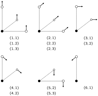
Figure 2: Symbolical sketch of the explicit compass solution in (109)-(130). In total 13 suitably prepared test bodies (hollow circles) are needed to determine all curvature components. The reference body is denoted by the black circle. Note that with the standard deviation equation all ${}^{(1\dots 6)}u^{a}$, but only ${}^{(1\dots 3)}\eta^{a}$ are needed in the solution.

IV.2.2 Vacuum spacetime

In vacuum the number of independent components of the curvature is reduced to the 10 components of the Weyl tensor $C_{abcd}$. Replacing $R_{abcd}$ in the compass solution (109)-(130), and taking into account the symmetries of Weyl we may use a reduced compass setup to completely determine the gravitational field, i.e.

$$01:C_{1010} = \frac{3}{4}{}^{(1,1)}A_{1}c^{-2}_{10},$$ (131)

$$02:C_{2010} = \frac{3}{4}{}^{(1,1)}A_{2}c^{-2}_{10},$$ (132)

$$03:C_{3010} = \frac{3}{4}{}^{(1,1)}A_{3}c^{-2}_{10},$$ (133)

$$04:C_{2020} = \frac{3}{4}{}^{(1,2)}A_{2}c^{-2}_{10},$$ (134)

$$05:C_{3020} = \frac{3}{4}{}^{(1,2)}A_{3}c^{-2}_{10},$$ (135)

$$06:C_{2110} = \frac{3}{4}{}^{(2,1)}A_{2}c^{-1}_{21}c^{-1}_{20}-C_{2010}c^{-1}_{21}c_{20},$$ (136)

$$07:C_{3110} = \frac{3}{4}{}^{(2,1)}A_{3}c^{-1}_{21}c^{-1}_{20}-C_{3010}c^{-1}_{21}c_{20},$$ (137)

$$08:C_{0212} = \frac{3}{4}{}^{(3,1)}A_{0}c^{-2}_{32}+C_{2010}c^{-1}_{32}c_{30},$$ (138)

$$09:C_{0231} = \frac{1}{4}{}^{(4,1)}A_{2}c^{-1}_{40}c^{-1}_{43}-\frac{1}{4}{}^{(2,2)}A_{3}c^{-1}_{20}c^{-1}_{21}$$ (139)

$$+\frac{1}{3}C_{3020}\big{(}c_{20}c^{-1}_{21}+c_{21}c^{-1}_{20}\big{)}$$

$$-\frac{1}{3}C_{2010}\big{(}c_{40}c^{-1}_{43}+c_{43}c^{-1}_{40}\big{)},$$

$$10:C_{0312} = \frac{1}{4}{}^{(4,1)}A_{2}c^{-1}_{40}c^{-1}_{42}+\frac{1}{2}{}^{(2,2)}A_{3}c^{-1}_{20}c^{-1}_{21}$$ (140)

$$-\frac{2}{3}C_{3020}\big{(}c_{20}c^{-1}_{21}+c_{21}c^{-1}_{20}\big{)}$$

$$+\frac{1}{3}C_{2010}\big{(}c_{40}c^{-1}_{43}+c_{43}c^{-1}_{40}\big{)}.$$

All the other components of the Weyl tensor are obtained from the above by making use of the double-self-duality property $C_{abcd}=-\frac{1}{4}\epsilon_{abef}\epsilon_{cdgh}C^{efgh}$, where $\epsilon_{abcd}$ is the totally antisymmetric Levi-Civita tensor with $\epsilon_{0123}=1$, and the Ricci identity. See fig. 3 for a sketch of the solution.

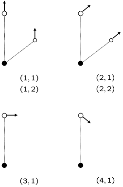
Figure 3: Symbolical sketch of the explicit compass solution in (131)-(140) for the vacuum case. In total 6 suitably prepared test bodies (hollow circles) are needed to determine all components of the Weyl tensor. The reference body is denoted by the black circle. Note that in vacuum, with the standard deviation equation, all ${}^{(1\dots 4)}u^{a}$, but only ${}^{(1\dots 2)}\eta^{a}$ are needed in the solution.

IV.3 Generalized deviation equation

Let us come back to the generalized deviation equation derived in the first part of the work. In particular the generalized equation with synchronous parametrization for geodesic curves, i.e. (49). Considering this equation at first order, one interesting question is whether it allows for a determination of the curvature with a smaller number of test bodies than the standard deviation equation considered in section IV.1.

Rewriting (49) at first order in normal coordinates yields:

$$\frac{d^{2}}{ds^{2}}\eta_{a} \stackrel{{\scriptstyle|_{Y}}}{{=}} \frac{4}{3}R_{abcd}u^{b}\eta^{c}u^{d}+2R_{abcd}\frac{d\eta^{b}}{ds}\eta^{c}u^{d}.$$ (141)

The apparent difference w.r.t. to (58) is that now the velocities of the individual test bodies come into play.

IV.4 Generalized compass setup

The lhs of (141) are the measured accelerations and in the following we refer to them by ${}^{(m,n,p)}A_{a}$. In other words, for $(m)$ compasses, with ${}^{(m)}u^{a}$ velocities, and $(n)$ test bodies, which can move individually with $(p)$ velocities in one compass, we have the following set of equations:

$${}^{(m,n,p)}A_{a} \stackrel{{\scriptstyle|_{Y}}}{{=}} \frac{4}{3}R_{abcd}\,{}^{(m)}u^{b}\,{}^{(n)}\eta^{c}\,{}^{(m)}u^{d}$$ (142)

$$+2R_{abcd}\,{}^{(p)}\!\stackrel{{\scriptstyle\circ}}{{\eta}}\!{}^{b}\,{}^{(n)}\eta^{c}\,{}^{(m)}u^{d}.$$

Here we used the shortcut notation “$\stackrel{{\scriptstyle\circ}}{{\eta}}\!{}^{a}$”$=d\eta^{a}/ds$ for the standard total derivative. What remains to be chosen, apart from the $(n=1\dots 5)$ positions of bodies in one compass, the $(m=1\dots 6)$ actual directions in which each compass / observer shall move, are the $(p=0\dots 6)$ individual velocities of the bodies. Of course in the end we want to minimize all three numbers, i.e. $(m)$, $(n)$, and $(p)$ which are needed to determine all curvature components.

$${}^{(1)}\!\stackrel{{\scriptstyle\circ}}{{\eta}}\!{}^{a}=\left(\begin{array}[]{c}d_{10}\\ 0\\ 0\\ 0\\ \end{array}\right),{}^{(2)}\!\stackrel{{\scriptstyle\circ}}{{\eta}}\!{}^{a}=\left(\begin{array}[]{c}d_{20}\\ d_{21}\\ 0\\ 0\\ \end{array}\right),{}^{(3)}\!\stackrel{{\scriptstyle\circ}}{{\eta}}\!{}^{a}=\left(\begin{array}[]{c}d_{30}\\ 0\\ d_{32}\\ 0\\ \end{array}\right),$$ (155)

$${}^{(4)}\!\stackrel{{\scriptstyle\circ}}{{\eta}}\!{}^{a}=\left(\begin{array}[]{c}d_{40}\\ 0\\ 0\\ d_{43}\\ \end{array}\right),{}^{(5)}\!\stackrel{{\scriptstyle\circ}}{{\eta}}\!{}^{a}=\left(\begin{array}[]{c}d_{50}\\ d_{51}\\ d_{52}\\ 0\\ \end{array}\right),{}^{(6)}\!\stackrel{{\scriptstyle\circ}}{{\eta}}\!{}^{a}=\left(\begin{array}[]{c}d_{60}\\ 0\\ d_{62}\\ d_{63}\\ \end{array}\right).$$ (168)

(169)

The $d_{(p)a}$ here are just constants, chosen appropriately to ensure the normalization of the 4-velocity of each test body. Note that in order to recover the results from the previous compass setup in the context of the standard deviation equation, we have just have to choose

$${}^{(0)}\!\stackrel{{\scriptstyle\circ}}{{\eta}}\!{}^{a}=\left(\begin{array}[]{c}0\\ 0\\ 0\\ 0\\ \end{array}\right).$$ (174)

IV.4.1 Explicit curvature components

Similarly to Sec. IV.2, the 20 independent components of the curvature tensor can be explicitly determined in terms of the accelerations ${}^{(m,n,p)}A_{a}$ and velocities ${}^{(m)}u^{a}$ via the deviation equation (142) by using the compass configuration given in (80), (108), and (169). The result reads as follows

$$01:R_{1010} = \frac{3}{4}{}^{(1,1,0)}A_{1}c^{-2}_{10},$$ (175)

$$02:R_{2010} = \frac{3}{4}{}^{(1,1,0)}A_{2}c^{-2}_{10},$$ (176)

$$03:R_{3010} = \frac{3}{4}{}^{(1,1,0)}A_{3}c^{-2}_{10},$$ (177)

$$04:R_{2110} = \frac{1}{2}{}^{(1,1,2)}A_{2}d^{-1}_{21}c^{-1}_{10}-\left(\frac{2}{3}d^{-1}_{21}c_{10}+d_{20}d^{-1}_{21}\right)R_{2010},$$ (178)

$$05:R_{3110} = \frac{1}{2}{}^{(1,1,2)}A_{3}d^{-1}_{21}c^{-1}_{10}-\left(\frac{2}{3}d^{-1}_{21}c_{10}+d_{20}d^{-1}_{21}\right)R_{3010},$$ (179)

$$06:R_{3210} = \frac{1}{2}{}^{(1,1,3)}A_{3}d^{-1}_{32}c^{-1}_{10}-\left(\frac{2}{3}d^{-1}_{32}c_{10}+d_{30}d^{-1}_{32}\right)R_{3010},$$ (180)

$$07:R_{2020} = \frac{3}{4}{}^{(1,2,0)}A_{2}c^{-2}_{10},$$ (181)

$$08:R_{3020} = \frac{3}{4}{}^{(1,2,0)}A_{3}c^{-2}_{10},$$ (182)

$$09:R_{2120} = \frac{1}{2}{}^{(1,2,2)}A_{2}d^{-1}_{21}c^{-1}_{10}-\left(\frac{2}{3}d^{-1}_{21}c_{10}+d_{20}d^{-1}_{21}\right)R_{2020},$$ (183)

$$10:R_{3120} = \frac{1}{2}{}^{(1,2,2)}A_{3}d^{-1}_{21}c^{-1}_{10}-\left(\frac{2}{3}d^{-1}_{21}c_{10}+d_{20}d^{-1}_{21}\right)R_{3020},$$ (184)

$$11:R_{3220} = \frac{1}{2}{}^{(1,2,3)}A_{3}d^{-1}_{32}c^{-1}_{10}-\left(\frac{2}{3}d^{-1}_{32}c_{10}+d_{30}d^{-1}_{32}\right)R_{3020},$$ (185)

$$12:R_{3030} = \frac{3}{4}{}^{(1,3,0)}A_{3}c^{-2}_{10},$$ (186)

$$13:R_{2130} = \frac{1}{2}{}^{(1,3,2)}A_{2}d^{-1}_{21}c^{-1}_{10}-\left(\frac{2}{3}d^{-1}_{21}c_{10}+d_{20}d^{-1}_{21}\right)R_{2030},$$ (187)

$$14:R_{3130} = \frac{1}{2}{}^{(1,3,2)}A_{3}d^{-1}_{21}c^{-1}_{10}-\left(\frac{2}{3}d^{-1}_{21}c_{10}+d_{20}d^{-1}_{21}\right)R_{3030},$$ (188)

$$15:R_{3230} = \frac{1}{2}{}^{(1,3,3)}A_{3}d^{-1}_{32}c^{-1}_{10}-\left(\frac{2}{3}d^{-1}_{32}c_{10}+d_{30}d^{-1}_{32}\right)R_{3030},$$ (189)

$$16:R_{2121} = \frac{3}{4}{}^{(2,2,0)}A_{2}c^{-2}_{21}-R_{2020}c^{2}_{20}c^{-2}_{21}-2R_{2120}c_{20}c^{-1}_{21},$$ (190)

$$17:R_{3121} = \frac{3}{4}{}^{(2,2,0)}A_{3}c^{-2}_{21}-R_{3020}c^{2}_{20}c^{-2}_{21}-\left(R_{3021}+R_{3120}\right)c_{20}c^{-1}_{21},$$ (191)

$$18:R_{3221} = \frac{1}{2}{}^{(2,2,3)}A_{3}d^{-1}_{32}c^{-1}_{21}-\left(\frac{2}{3}d^{-1}_{32}c_{20}+d_{30}d^{-1}_{32}\right)R_{3021}-\left(\frac{2}{3}d^{-1}_{32}c^{-1}_{21}c^{2}_{20}+d^{-1}_{32}d_{30}c^{-1}_{21}c_{20}\right)R_{3020}$$ (192)

$$-\frac{2}{3}R_{3120}d^{-1}_{32}c_{20}-\frac{2}{3}R_{3121}d^{-1}_{32}c_{21}-R_{3220}c^{-1}_{21}c_{20},$$

$$19:R_{3131} = \frac{3}{4}{}^{(2,3,0)}A_{3}c^{-2}_{21}-R_{3030}c_{20}c^{-2}_{21}-2R_{3130}c_{20}c^{-1}_{21},$$ (193)

$$20:R_{3231} = \frac{1}{2}{}^{(2,3,3)}A_{3}d^{-1}_{32}c^{-1}_{21}-\left(\frac{4}{3}d^{-1}_{32}c_{20}+d^{-1}_{32}d_{30}\right)R_{3031}-\left(\frac{2}{3}d^{-1}_{32}c^{-1}_{21}c^{2}_{20}+d^{-1}_{32}d_{30}c^{-1}_{21}c_{20}\right)R_{3030}$$ (194)

$$-\frac{2}{3}d^{-1}_{32}c_{21}R_{3131}-R_{3230}c^{-1}_{21}c_{20},$$

By examination of the components given in (175)-(194), we infer that for a full determination of the curvature by means of the generalized deviation equation one again needs 13 test bodies. See fig. 4 for a sketch of the solution.

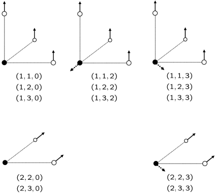
Figure 4: Symbolical sketch of the explicit compass solution in (175)-(194). Again, in total 13 suitably prepared test bodies (hollow circles) are needed to determine all curvature components. The reference body is denoted by the black circle. Note that with the generalized deviation equation only ${}^{(1\dots 2)}u^{a}$, ${}^{(1\dots 3)}\eta^{a}$, and ${}^{(2\dots 3)}\!\stackrel{{\scriptstyle\circ}}{{\eta}}\!{}^{a}$ are needed in the solution.

IV.4.2 Vacuum spacetime

Table 1: Number of required bodies in a compass setup for a full determination of the gravitational field, i.e. 20 components of $R_{abcd}$ in a general spacetime, and 10 components of $C_{abcd}$ in vacuum.

	Spacetime
	General	Vacuum
Standard deviation equation	13	6
Generalized deviation equation	13	5

By replacing $R_{abcd}$ in the compass solution (175)-(194), and taking into account the symmetries of Weyl we may use a reduced compass setup to completely determine the gravitational field, this time by means of the generalized deviation equation. Explicitly, one ends up with

$$01:C_{1010} = \frac{3}{4}{}^{(1,1,0)}A_{1}c^{-2}_{10},$$ (195)

$$02:C_{2010} = \frac{3}{4}{}^{(1,1,0)}A_{2}c^{-2}_{10},$$ (196)

$$03:C_{3010} = \frac{3}{4}{}^{(1,1,0)}A_{3}c^{-2}_{10},$$ (197)

$$04:C_{2110} = \frac{1}{2}{}^{(1,1,2)}A_{2}d^{-1}_{21}c^{-1}_{10}$$ (198)

$$-\left(\frac{2}{3}d^{-1}_{21}c_{10}+d_{20}d^{-1}_{21}\right)C_{2010},$$

$$05:C_{3110} = \frac{1}{2}{}^{(1,1,2)}A_{3}d^{-1}_{21}c^{-1}_{10}$$ (199)

$$-\left(\frac{2}{3}d^{-1}_{21}c_{10}+d_{20}d^{-1}_{21}\right)C_{3010},$$

$$06:C_{3210} = \frac{1}{2}{}^{(1,1,3)}A_{3}d^{-1}_{32}c^{-1}_{10}$$ (200)

$$-\left(\frac{2}{3}d^{-1}_{32}c_{10}+d_{30}d^{-1}_{32}\right)C_{3010},$$

$$07:C_{2020} = \frac{3}{4}{}^{(1,2,0)}A_{2}c^{-2}_{10},$$ (201)

$$08:C_{3020} = \frac{3}{4}{}^{(1,2,0)}A_{3}c^{-2}_{10},$$ (202)

$$09:C_{2120} = \frac{1}{2}{}^{(1,2,2)}A_{2}d^{-1}_{21}c^{-1}_{10}$$ (203)

$$-\left(\frac{2}{3}d^{-1}_{21}c_{10}+d_{20}d^{-1}_{21}\right)C_{2020},$$

$$10:C_{3120} = \frac{1}{2}{}^{(1,2,2)}A_{3}d^{-1}_{21}c^{-1}_{10}$$ (204)

$$-\left(\frac{2}{3}d^{-1}_{21}c_{10}+d_{20}d^{-1}_{21}\right)C_{3020}.$$

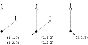
Figure 5: Symbolical sketch of the explicit compass solution in (195)-(204) for the vacuum case. In total 5 suitably prepared test bodies (hollow circles) are needed to determine all components of the Weyl tensor. The reference body is denoted by the black circle. Note that in vacuum, with the generalized deviation equation, only ${}^{(1)}u^{a}$, ${}^{(1\dots 2)}\eta^{a}$, and ${}^{(2\dots 3)}\!\stackrel{{\scriptstyle\circ}}{{\eta}}\!{}^{a}$ are needed in the solution.

See fig. 5 for a sketch of the solution. Table 1 contains an overview of the number of required test bodies in different compass setups and in general as well as in vacuum spacetimes.

V Conclusion

In this work we derived a generalized covariant deviation equation in the framework of Synge’s world function approach. It should be stressed that our exact deviation equation in (9) is valid for arbitrary world lines and in general background spacetimes. In the subsequent analysis we provided a systematic expansion of the exact deviation equation up to the third order in the world function (35). This equation can be viewed as a generalization of the well-known geodesic deviation equation, to which it was shown to reduce under the right assumptions. As we have shown in detail, our results encompass several suggestions for a generalized deviation equation from the literature as special cases, and therefore may serve a unified framework for further studies.

In a subsequent analysis we have shown how deviation equations can be used to determine the curvature of spacetime. For this we extended the notion of a gravitational compass Szekeres (1965) and worked out compass setups for general as well as for vacuum spacetimes. One setup is based on the standard geodesic deviation equation (39), and another is based on the next order generalization given in (49) which goes beyond the linearized case. For both cases we provided the explicit compass solution which allows for a full determination of the curvature.

In contrast to the general considerations in Synge (1960); Szekeres (1965) we give an explicit exact solution for the compass setup. With the standard deviation equation, as well as with the generalized deviation equation, we need at least 13 test bodies to determine all curvature components in a general spacetime. For the standard deviation we therefore obtain the same number of bodies as in Ciufolini and Demianski (1986), however it is worthwhile to note that no explicit solution was given in Ciufolini and Demianski (1986) for a non-vacuum spacetime. In the case of a generalized deviation equation our findings are at odds with the results in Ciufolini and Demianski (1986). However, this discrepancy in the generalized case comes as no surprise since the generalized equation used in Ciufolini and Demianski (1986) – which was previously derived in Ciufolini (1986) – differs from our equation. In vacuum spacetimes, we have explicitly shown that the number of required test bodies is reduced to 6, for the standard deviation equation, and to 5, for the generalized deviation equation.

Furthermore, it is interesting to note that in the case of the standard deviation equation, the opinion of the authors Synge (1960); Szekeres (1965) differs when it comes to the number of required test bodies. This seems to be related to the counting scheme and the interpretation of the notion of a compass. Since no explicit compass solutions were given in Synge (1960); Szekeres (1965), one cannot make a comparison to our results. In the case of Ciufolini and Demianski (1986), we were not able to verify that the given solution does fulfill the compass equations derived in that work. However, the agreement on the number of required bodies in combination with the standard deviation is reassuring.

In summary, we have explicitly shown how deviation equations can be used to measure the gravitational field. Our results are of direct operational relevance and form the basis for many experiments. Important applications range from the description of gravitational wave detectors to the study of satellite configurations for gravitational field mapping in relativistic geodesy. An interesting question is whether a further reduction of the number of required test bodies for certain experiments is possible. A systematic analysis of the practical applications of generalized deviation equations, including the gravitation wave detection, will be presented elsewhere.

Appendix A Notations and conventions

Table 2: Directory of symbols.

Symbol	Explanation
Geometrical quantities
$g_{ab}$	Metric
$\sqrt{-g}$	Determinant of the metric
$\delta^{a}_{b}$	Kronecker symbol
$\epsilon_{abcd}$	Levi-Civita symbol
$x^{a}$, $s$	Coordinates, proper time
$\Gamma_{ab}{}^{c}$	Connection
${}^{\ast}\Gamma_{ab\dots}{}^{c}$	Deriv. conn. (normal coords.)
$R_{abc}{}^{d}$, $C_{abc}{}^{d}$	Riemann, Weyl curvature
$\sigma$	World function
$\eta^{y}$	Deviation vector
$g^{y_{0}}{}_{x_{0}}$	Parallel propagator
Misc
$Y(t),X(t)$	(Reference) world line
$u^{a}$	Velocity
$a^{b}$	Acceleration
$K^{x}{}_{y},H^{x}{}_{y}$	Jacobi propagators
${}^{(m,n)}A_{a}$, ${}^{(m,n,p)}A_{a}$	Accelerations of
	compass constituents
Auxiliary quantities
$\alpha^{y_{0}}{}_{y_{1}\dots y_{n}}$, $\beta^{y_{0}}{}_{y_{1}\dots y_{n}}$, $\gamma^{y_{0}}{}_{y_{1}\dots y_{n}}$	Expansion coefficients
$c_{(m)a}$, $d_{(m)a}$	Constants
$\phi^{y_{1}}{}_{y_{2}\dots}$, $\lambda^{y_{1}}{}_{y_{2}\dots}$, $\mu^{y_{1}}{}_{y_{2}\dots}$,	Abbreviations
$\Delta_{i_{1}\dots}$, $\Xi_{i_{1}\dots}$
Operators
$\partial_{i}$, $\nabla_{i}$	(Partial, covariant) derivative
$\frac{D}{ds}=$“$\dot{\phantom{a}}$”	Total cov. derivative
$\frac{d}{ds}=$“$\stackrel{{\scriptstyle\circ}}{{\phantom{a}}}$”	Total derivative
“$[\dots]$”	Coincidence limit

Our conventions for the Riemann curvature are as follows:

$$2T^{c_{1}\dots c_{k}}{}_{d_{1}\dots d_{l};[ba]}\equiv 2\nabla_{[a}\nabla_{b]}T^{c_{1}\dots c_{k}}{}_{d_{1}\dots d_{l}}$$ (205)

$$= \sum^{k}_{i=1}R_{abe}{}^{c_{i}}T^{c_{1}\dots e\dots c_{k}}{}_{d_{1}\dots d_{l}}$$

$$-\sum^{l}_{j=1}R_{abd_{j}}{}^{e}T^{c_{1}\dots c_{k}}{}_{d_{1}\dots e\dots d_{l}}.$$

The Ricci tensor is introduced by $R_{ij}=R_{kij}{}^{k}$, and the curvature scalar is $R=g^{ij}R_{ij}$. The signature of the spacetime metric is assumed to be $(+1,-1,-1,-1)$.

In the following, we summarize some of the frequently used formulas in the context of the bitensor formalism [in particular for the world function $\sigma(x,y)$], see, e.g., Synge (1960); DeWitt and Brehme (1960); Poisson et al. (2011) for the corresponding derivations. Note that our curvature conventions differ from those in Synge (1960); Poisson et al. (2011). Indices attached to the world function always denote covariant derivatives, at the given point, i.e. $\sigma_{y}:=\nabla_{y}\sigma$; hence, we do not make explicit use of the semicolon in case of the world function. We start by stating, without proof, the following useful rule for a bitensor $B$ with arbitrary indices at different points (here just denoted by dots):

$$\left[B_{\dots}\right]_{;y}=\left[B_{\dots;y}\right]+\left[B_{\dots;x}\right].$$ (206)

Here a coincidence limit of a bitensor $B_{\dots}(x,y)$ is a tensor

$$\left[B_{\dots}\right]=\lim\limits_{x\rightarrow y}\,B_{\dots}(x,y),$$ (207)

determined at $y$. Furthermore, we collect the following useful identities:

$$\sigma_{y_{0}y_{1}x_{0}y_{2}x_{1}}=\sigma_{y_{0}y_{1}y_{2}x_{0}x_{1}}=\sigma_{x_{0}x_{1}y_{0}y_{1}y_{2}},$$ (208)

$$g^{x_{1}x_{2}}\sigma_{x_{1}}\sigma_{x_{2}}=2\sigma=g^{y_{1}y_{2}}\sigma_{y_{1}}\sigma_{y_{2}},$$ (209)

$$\left[\sigma\right]=0,\quad\left[\sigma_{x}\right]=\left[\sigma_{y}\right]=0,$$ (210)

$$\left[\sigma_{x_{1}x_{2}}\right]=\left[\sigma_{y_{1}y_{2}}\right]=g_{y_{1}y_{2}},$$ (211)

$$\left[\sigma_{x_{1}y_{2}}\right]=\left[\sigma_{y_{1}x_{2}}\right]=-g_{y_{1}y_{2}},$$ (212)

$$\left[\sigma_{x_{1}x_{2}x_{3}}\right]=\left[\sigma_{x_{1}x_{2}y_{3}}\right]=\left[\sigma_{x_{1}y_{2}y_{3}}\right]=\left[\sigma_{y_{1}y_{2}y_{3}}\right]=0,$$

(213)

$$\left[g^{x_{0}}{}_{y_{1}}\right]=\delta^{y_{0}}{}_{y_{1}},\quad\left[g^{x_{0}}{}_{y_{1};x_{2}}\right]=\left[g^{x_{0}}{}_{y_{1};y_{2}}\right]=0,$$ (214)

$$\left[g^{x_{0}}{}_{y_{1};x_{2}x_{3}}\right]=\frac{1}{2}R^{y_{0}}{}_{y_{1}y_{2}y_{3}}.$$ (215)

Appendix B Normal coordinates

Here we provide the explicit expressions of the derivatives of the Riemannian connection $\Gamma_{i_{1}\dots i_{N}ij}{}^{k}:=\partial_{i_{1}}\dots\partial_{i_{N}}\Gamma_{ij}{}^{k}$ in normal coordinates.

The list of the lowest derivatives for $N=0,1,2,3$ reads as follows:

$${}^{\ast}\Gamma_{ij}{}^{k} = 0,$$ (216)

$${}^{\ast}\Gamma_{i_{1}ij}{}^{k} = {\frac{2}{3}}\,R_{i_{1}(ij)}{}^{k},$$ (217)

$${}^{\ast}\Gamma_{i_{1}i_{2}ij}{}^{k} = {\frac{1}{6}}\left[5\nabla_{(i_{1}}R_{i_{2})(ij)}{}^{k}-\nabla_{(i}R_{j)(i_{1}i_{2})}{}^{k}\right],$$ (218)

$${}^{\ast}\Gamma_{i_{1}i_{2}i_{3}ij}{}^{k} = {\frac{3}{20}}\left[6\nabla_{(i_{1}}\nabla_{i_{2}}R_{i_{3})(ij)}{}^{k}-\nabla_{i}\nabla_{(i_{1}}R_{|j|i_{2}i_{3})}{}^{k}\right.$$ (219)

$$\left.-\nabla_{j}\nabla_{(i_{1}}R_{|i|i_{2}i_{3})}{}^{k}\right]+{\frac{4}{15}}\,R_{p(i_{1}i_{2}}{}^{k}\,R_{i_{3})(ij)}{}^{p}$$

$$+\frac{1}{2}\left[R_{p(i_{1}i_{2}}{}^{k}\,R_{i_{3})(ij)}{}^{p}-R_{i(i_{1}i_{2}}{}^{p}\,R_{i_{3})(jp)}{}^{k}\right.$$

$$\left.-R_{j(i_{1}i_{2}}{}^{p}\,R_{i_{3})(ip)}{}^{k}\right]+\frac{1}{10}\left[R_{i(i_{1}i_{2}}{}^{p}\,R_{i_{3})jp}{}^{k}\right.$$

$$\left.+R_{j(i_{1}i_{2}}{}^{p}\,R_{i_{3})ip}{}^{k}\right].$$

The parentheses denote the symmetrization over the enclosed indices; indices between the vertical lines are excluded from the symmetrization. As a check, from these formulas we can derive the symmetrized derivatives of the connection which are better known in the literature (see, e.g., Petrov Petrov (1969)):

$${}^{\ast}\Gamma_{(i_{1}i)j}{}^{k} = -\,{\frac{1}{3}}\,R_{j(i_{1}i)}{}^{k},$$ (220)

$${}^{\ast}\Gamma_{(i_{1}i_{2}i)j}{}^{k} = -\,{\frac{1}{2}}\,\nabla_{(i_{1}}R_{|j|i_{2}i)}{}^{k},$$ (221)

$${}^{\ast}\Gamma_{(i_{1}i_{2}i_{3}i)j}{}^{k} = -\,{\frac{3}{5}}\nabla_{(i_{1}}\nabla_{i_{2}}R_{|j|i_{3}i)}{}^{k}$$ (222)

$$-{\frac{2}{15}}\,R_{p(i_{1}i_{2}}{}^{k}\,R_{|j|i_{3}i)}{}^{p}.$$

It is worthwhile to note that the symmetrization of the two last lines in (219) over $(i_{1}i_{2}i_{3}i)$ yields zero.

The above formulas can be derived as follows. The derivatives of the connection ${}^{\ast}\Gamma_{i_{1}\cdots i_{N}\,ij}{}^{k}$ satisfy the algebraic equations

$${}^{\ast}\Gamma_{i_{1}i_{2}\cdots i_{N}\,ij}{}^{k}-{}^{\ast}\Gamma_{ii_{2}\cdots i_{N}\,i_{1}j}{}^{k}=\Delta_{i_{1}iji_{2}\cdots i_{N}}{}^{k},$$ (223)

where $\Delta_{i_{1}iji_{2}\cdots i_{N}}{}^{k}$ are the tensors with the symmetry properties

$$\Delta_{i_{1}iji_{2}\cdots i_{N}}{}^{k} = -\,\Delta_{ii_{1}ji_{2}\cdots i_{N}}{}^{k},$$ (224)

$$\Delta_{i_{1}iji_{2}\cdots i_{N}}{}^{k} = \Delta_{ii_{1}j(i_{2}\cdots i_{N})}{}^{k},$$ (225)

$$\Delta_{[i_{1}ij]i_{2}\cdots i_{N}}{}^{k} = 0,$$ (226)

$$\Delta_{[i_{1}i|j|i_{2}]\cdots i_{N}}{}^{k} = 0.$$ (227)

That is, these tensors are skew-symmetric in the first two indices and totally symmetric in the last $N-1$ indices (these properties are thus consistent with the symmetry properties of the left-hand side of the equation (223)), and in addition, the antisymmetrization over the first three indices and over the first pair and the fourth index vanishes. Using these symmetry properties, one can solve the equation (223) with respect to the derivatives of the connection. In symbolic form, the general solution (for any $N$) reads

$${}^{\ast}\Gamma_{i_{1}i_{2}\cdots i_{N}\,ij}{}^{k} = \frac{1}{K}\left[(K-1)\Delta_{\rm perm}{}^{k}+(K-2)\Delta_{\rm perm}{}^{k}\right.$$ (228)

$$\left.+\cdots+\Delta_{\rm perm}{}^{k}\right],$$

where $K=(N+2)(N+1)/2$ and the right-hand side contains $(K-1)$ terms in which the $(N+2)$ lower indices of $\Delta$’s are permuted in accordance with a certain rule. Actually, the determination of this permutation rule is a highly nontrivial problem which is related to the famous theorem of Desargues, as was shown by Veblen Veblen (1922).

We will only give the solutions for the case of $N=1,2,3,4$:

$${}^{\ast}\Gamma_{i_{1}ij}{}^{k} = {\frac{1}{3}}\left[2\Delta_{i_{1}ji}{}^{k}+\Delta_{jii_{1}}{}^{k}\right],$$ (229)

$${}^{\ast}\Gamma_{i_{1}i_{2}ij}{}^{k} = {\frac{1}{6}}\left[5\Delta_{i_{1}jii_{2}}{}^{k}+4\Delta_{jii_{1}i_{2}}{}^{k}+3\Delta_{i_{2}ji_{1}i}{}^{k}\right.$$ (230)

$$\left.+\,2\Delta_{ii_{1}i_{2}j}{}^{k}+\Delta_{jii_{2}i_{1}}{}^{k}\right],$$

$${}^{\ast}\Gamma_{i_{1}i_{2}i_{3}ij}{}^{k} = {\frac{1}{10}}\left[9\Delta_{i_{1}jii_{2}i_{3}}{}^{k}+8\Delta_{jii_{1}i_{2}i_{3}}{}^{k}\right.$$ (231)

$$+7\Delta_{i_{2}ji_{1}ii_{3}}{}^{k}+\,6\Delta_{ii_{1}i_{2}ji_{3}}{}^{k}$$

$$+5\Delta_{jii_{2}i_{1}i_{3}}{}^{k}+4\Delta_{i_{3}ji_{2}ii_{1}}{}^{k}$$

$$+\,3\Delta_{i_{1}i_{2}i_{3}ji}{}^{k}+2\Delta_{ii_{1}i_{3}i_{2}j}{}^{k}$$

$$+\,\left.\Delta_{jii_{3}i_{1}i_{2}}{}^{k}\right],$$

$${}^{\ast}\Gamma_{i_{1}i_{2}i_{3}i_{4}ij}{}^{k} = {\frac{1}{15}}\left[14\Delta_{i_{1}jii_{2}i_{3}i_{4}}{}^{k}+13\Delta_{jii_{1}i_{2}i_{3}i_{4}}{}^{k}\right.$$ (232)

$$+\,12\Delta_{i_{2}ji_{1}ii_{3}i_{4}}{}^{k}+11\Delta_{ii_{1}i_{2}ji_{3}i_{4}}{}^{k}$$

$$+\,10\Delta_{jii_{2}i_{1}i_{3}i_{4}}{}^{k}+9\Delta_{i_{3}ji_{2}ii_{1}i_{4}}{}^{k}$$

$$+\,8\Delta_{i_{1}i_{2}i_{3}jii_{4}}{}^{k}+7\Delta_{ii_{1}i_{3}i_{2}ji_{4}}{}^{k}$$

$$+6\Delta_{jii_{3}i_{1}i_{2}i_{4}}{}^{k}+\,5\Delta_{i_{4}ji_{3}ii_{1}i_{2}}{}^{k}$$

$$+4\Delta_{i_{2}i_{3}i_{4}jii_{1}}{}^{k}+3\Delta_{i_{1}i_{2}i_{4}i_{3}ji}{}^{k}$$

$$\left.+2\Delta_{ii_{1}i_{4}i_{2}i_{3}j}{}^{k}+\Delta_{jii_{4}i_{1}i_{2}i_{3}}{}^{k}\right].$$

By differentiating covariantly the curvature tensor $R_{ijl}{}^{k}$, one can straightforwardly identify the $\Delta$’s with the polynomials built from the curvature and its derivatives. Explicitly, we have

$$\Delta_{i_{1}ij}{}^{k} = R_{i_{1}ij}{}^{k},$$ (233)

$$\Delta_{i_{1}iji_{2}}{}^{k} = \nabla_{i_{2}}R_{i_{1}ij}{}^{k},$$ (234)

$$\Delta_{i_{1}iji_{2}i_{3}}{}^{k} = \nabla_{(i_{2}}\nabla_{i_{3})}R_{i_{1}ij}{}^{k}+\Xi_{i_{1}iji_{2}i_{3}}{}^{k},$$ (235)

where the quadratic in curvature contraction reads

$$\Xi_{i_{1}iji_{2}i_{3}}{}^{k} ={\frac{1}{3}}\left[R_{j(i_{2}i_{3})}{}^{p}\,R_{ii_{1}p}{}^{k}-R_{p(i_{2}i_{3})}{}^{k}\,R_{ii_{1}j}{}^{p}\right.$$ (236)

$$+\left.R_{i(i_{2}i_{3})}{}^{p}\,R_{pi_{1}j}{}^{k}-R_{i_{1}(i_{2}i_{3})}{}^{p}\,R_{pij}{}^{k}\right]$$

$$+\,{\frac{4}{9}}\left[R_{i_{2}(ip)}{}^{k}\,R_{i_{3}(i_{1}j)}{}^{p}+R_{i_{3}(ip)}{}^{k}\,R_{i_{2}(i_{1}j)}{}^{p}\right.$$

$$-\left.R_{i_{2}(i_{1}p)}{}^{k}\,R_{i_{3}(ij)}{}^{p}-R_{i_{3}(i_{1}p)}{}^{k}\,R_{i_{2}(ij)}{}^{p}\right].$$

Inserting (233)-(236) into (229)-(231), we finally obtain the expressions (217)-(219).

It is worthwhile to mention that all the formulas derived here (in accordance with the general theory of normal coordinates Veblen (1922); Veblen and Thomas (1923); Thomas (1934)) are valid not only for the Riemannian Christoffel symbols but for an arbitrary symmetric connection $\Gamma_{ij}{}^{k}$ too. The explicit higher order results (219), (231), (232) and (236) are new.

A direct prescription how to calculate the derivatives of the connection is described in Avramidi (1991, 1995), although it seems impossible to give an explicit general formula. However, using the recursive prescriptions of Avramidi (1991, 1995), one can find the ${}^{\ast}\Gamma$’s for any $N$.

References

• Synge [1960] J. L. Synge. Relativity: The general theory. North-Holland, Amsterdam, 1960.
• DeWitt and Brehme [1960] B. S. DeWitt and R. W. Brehme. Radiation damping in a gravitational field. Ann. Phys. (N.Y.), 9:220, 1960.
• Dixon [1964] W. G. Dixon. A covariant multipole formalism for extended test bodies in General Relativity. Nuovo Cimento, 34:317, 1964.
• Dixon [1974] W. G. Dixon. Dynamics of extended bodies in General Relativity. III. Equations of motion. Phil. Trans. R. Soc. Lond. A, 277:59, 1974.
• Dixon [1979] W. G. Dixon. Extended bodies in General Relativity: Their description and motion. Proc. Int. School of Phys. Enrico Fermi LXVII, Ed. J. Ehlers, North Holland, Amsterdam, page 156, 1979.
• Dixon [2008] W. G. Dixon. Mathisson’s new mechanics: Its aims and realisation. Acta Phys. Pol. B Proc. Suppl., 1:27, 2008.
• Puetzfeld and Obukhov [2014] D. Puetzfeld and Yu. N. Obukhov. Equations of motion in metric-affine gravity: a covariant unified framework. Phys. Rev. D, 90:084034, 2014.
• Dixon [2015] W. G. Dixon. The New Mechanics of Myron Mathisson and its subsequent development. ”Equations of Motion in Relativistic Gravity”, D. Puetzfeld et. al. (eds.), Fundamental theories of Physics, Springer, 179:1, 2015.
• Obukhov and Puetzfeld [2015] Yu. N. Obukhov and D. Puetzfeld. Multipolar test body equations of motion in generalized gravity theories. ”Equations of Motion in Relativistic Gravity”, D. Puetzfeld et. al. (eds.), Fundamental theories of Physics, Springer, 179:67, 2015.
• Ottewill and Wardell [2011] A. C. Ottewill and B. Wardell. Transport equation approach to calculations of Hadamard Green functions and non-coincident DeWitt coefficients. Phys. Rev. D, 84:104039, 2011.
• Poisson et al. [2011] E. Poisson, A. Pound, and I. Vega. The motion of point particles in curved spacetime. Living Reviews in Relativity, 14(7), 2011.
• Szekeres [1965] P. Szekeres. The gravitational compass. J. Math. Phys., 6:1387, 1965.
• Plebański [1965] J. Plebański. Conformal geodesic deviations. Acta Phys. Pol., 28:141, 1965.
• Hodgkinson [1972] D. E. Hodgkinson. A modified theory of geodesic deviation. Gen. Rel. Grav., 3:351, 1972.
• Bażański [1974] S. L. Bażański. The relative energy of test particles in General Relativity. Nova Acta Leopoldina, 39:215, 1974.
• Hojman [1975] S. A. Hojman. Electromagnetic and gravitational interactions of a relativistic spherical top. PhD. thesis, Princeton University, 1975.
• Bażański [1976] S. L. Bażański. A geometric formulation of the Taylor theorem for curves on affine manifolds. J. Math. Phys. (N.Y.), 17:217, 1976.
• Bażański [1977a] S. L. Bażański. Kinematics of relative motion of test particles in general relativity. Ann. H. Poin. A, 27:115, 1977a.
• Bażański [1977b] S. L. Bażański. Dynamics of relative motion of test particles in general relativity. Ann. H. Poin. A, 27:145, 1977b.
• Novello et al. [1977] M. Novello, I. Damião Soares, and J. M. Salim. On Jacobi fields. Gen. Rel. Grav, 8:95, 1977.
• Aleksandrov and Piragas [1978] A. N. Aleksandrov and K. A. Piragas. Geodesic structure: I. Relative dynamics of geodesics. Theoretical and Mathematical Physics, 38:48, 1978.
• Manoff [1979] S. Manoff. Lie derivatives and deviation equations in Riemannian spaces. Gen. Rel. Grav, 11:189, 1979.
• Schattner and Trümper [1981] R. Schattner and M. Trümper. World vectors, Jacobi vectors and Jacobi one-forms on a manifold with a linear symmetric connection. J. Phys. A: Math. Gen., 14:2345, 1981.
• Swaminarayan and Safko [1983] N. S. Swaminarayan and J. L. Safko. A coordinate-free derivation of a generalized geodesic deviation equation. J. Math. Phys. (N.Y.), 24:883, 1983.
• Schutz [1985] B. Schutz. On generalized equations of geodesic deviation. In: Galaxies, Axisymmetric Systems, and Relativity, Ed. M.A.H. MacCallum, Cambridge University Press, Cambridge, 17:237, 1985.
• Kamran and Marck [1986] N. Kamran and J.-A. Marck. Parallel-propagated frame along the geodesics of the metrics admitting a Killing-Yano tensor. J. Math. Phys. (N.Y.), 27:1589, 1986.
• Ciufolini [1986] I. Ciufolini. Generalized geodesic deviation equation. Phys. Rev. D, 34:1014, 1986.
• Bażański and Kostyukovich [1987a] S. L. Bażański and N. N. Kostyukovich. Kinematics of relative motion of charged test particles in general relativity. I. The first electromagnetic deviation. Acta Phys. Pol. B, 18:601, 1987a.
• Bażański and Kostyukovich [1987b] S. L. Bażański and N. N. Kostyukovich. Kinematics of relative motion of charged test particles in general relativity. II. The second electromagnetic deviation. Acta Phys. Pol. B, 18:621, 1987b.
• Bażański [1989] S. L. Bażański. Hamilton-Jacobi formalism for geodesics and geodesic deviations. J. Math. Phys. (N.Y.), 30:1018, 1989.
• Vanzo [1992] L. Vanzo. A generalization of the equation of geodesic deviation. Nuovo Cim. B, 107:771, 1992.
• Roberts [1996] M. D. Roberts. The quantization of geodesic deviation. Gen. Rel. Grav, 28:1385, 1996.
• Kerner et al. [2001] R. Kerner, J. W. van Holten, and R. Colistete Jr. Relativistic epicycles: another approach to geodesic deviations. Class. Quantum Grav., 18:4725, 2001.
• Manoff [2001] S. Manoff. Deviation operator and deviation equations over spaces with affine connections and metrics. J. Geom. Phys., 39:337, 2001.
• van Holten [2002] J. W. van Holten. World-line deviations and epicycles. Int. J. Mod. Phys. A, 17:2764, 2002.
• Chicone and Mashhoon [2002] C. Chicone and B. Mashhoon. The generalized Jacobi equation. Class. Quant. Grav., 19:4231, 2002.
• Nieto et al. [2003] J. A. Nieto, J. Saucedo, and V.M. Villanueva. Relativistic top deviation equation and gravitational waves. Phys. Lett. A, 312:175, 2003.
• Mohseni [2004] M. Mohseni. World-line deviation and spinning particles. Phys. Lett. B, 587:133, 2004.
• Heydari-Fard et al. [2005] M. Heydari-Fard, M. Mohseni, and H. R. Sepangi. Worldline deviations of charged spinning particles. Phys. Lett. B, 626:230, 2005.
• Perlick [2008] V. Perlick. On the generalized Jacobi equation. Gen. Rel. Grav, 40:1029, 2008.
• Vines [2015] J. Vines. Geodesic deviation at higher orders via covariant bitensors. Gen. Rel. Grav, 47:59, 2015.
• Shirokov [1973] M. F. Shirokov. On one new effect of the Einsteinian theory of gravtiation. Gen. Rel. Grav, 4:131, 1973.
• Greenberg [1974] P. Greenberg. The equation of geodesic deviation in Newtonian theory and the oblateness of the Earth. Nuovo Cim. B, 24:272, 1974.
• Mashhoon [1975] B. Mashhoon. On tidal phenomena in a strong gravtitational field. Astrophys. J., 197:705, 1975.
• Mashhoon [1977] B. Mashhoon. Tidal radiation. Astrophys. J., 216:591, 1977.
• Tammelo [1977] R. Tammelo. Quadrupole Test Particle as a Detector of Gravitational Waves. Gen. Rel. Grav, 8:313, 1977.
• Dolan et al. [1980] P. Dolan, P. Choudhury, and J. L. Safko. A “constant of motion” for the geodesic deviation equation. J. Austral. Math. Soc. B, 22:28, 1980.
• Caviglia et al. [1982] G. Caviglia, C. Zordan, and F. Salmistraro. Equation of geodesic deviation and Killing tensors. Int. J. Theo. Phys., 21:391, 1982.
• Fuchs [1983] H. Fuchs. Solutions of the equations of geodesic deviation for static spherical symmetric space-times. Ann. Phys. (Leipzig), 495:231, 1983.
• Audretsch and Lämmerzahl [1983] J. Audretsch and C. Lämmerzahl. Local and nonlocal measurements of the Riemann tensor. Gen. Rel. Grav, 15:495, 1983.
• Tammelo [1984] R. Tammelo. On the physical significance of the second geodesic deviation. Phys. Lett. A, 106:227, 1984.
• Bażański [1986] S. L. Bażański. A method of solving the geodesic deviation equations. Proc. 4th Marcel Grossmann meeting on General Relativity, Ed. R. Ruffini, Elsevier (Amsterdam), page 1615, 1986.
• Ciufolini and Demianski [1986] I. Ciufolini and M. Demianski. How to measure the curvature of space-time. Phys. Rev. D, 34:1018, 1986.
• Bażański and Kostyukovich [1987c] S. L. Bażański and N. N. Kostyukovich. On first integrals of the electromagnetic deviation equations. Acta Phys. Pol. B, 18:983, 1987c.
• Bażański and Jaranowski [1989] S. L. Bażański and P. Jaranowski. Geodesic deviation in the Schwarzschild space-time. J. Math. Phys. (N.Y.), 30:1794, 1989.
• Fuchs [1990a] H. Fuchs. Paralleltransport and geodesic deviation in static spherically symmetric space-times. Astron. Nach., 311:219, 1990a.
• Fuchs [1990b] H. Fuchs. Deviation of circular geodesics in static spherically symmetric space-times. Astron. Nach., 311:271, 1990b.
• Mohseni and Sepangi [2000] M. Mohseni and H. R. Sepangi. Gravitational waves and spinning test particles. Class. Quant. Grav., 17:4615, 2000.
• Balakin et al. [2000] A. Balakin, J. W. van Holten, and R. Kerner. Motions and worldline deviations in Einstein Maxwell theory. Class. Quantum Grav., 17:5009, 2000.
• Colistete et al. [2002] R. Colistete, C. Leygnac, and R. Kerner. Higher-order geodesic deviations applied to the Kerr metric. Class. Quantum Grav., 19:4573, 2002.
• Biesiada [2003] M. Biesiada. Epicyclic orbital oscillations in Newton’s and Einstein’s gravity from the geodesic deviation equation. Gen. Rel. Grav., 35:1503, 2003.
• Baskaran and Grishchuk [2004] D. Baskaran and L. P. Grishchuk. Components of the gravitational force in the field of a gravitational wave. Class. Quantum Grav., 21:4041, 2004.
• Mullari and Tammelo [2006] T. Mullari and R. Tammelo. On the relativistic tidal effects in the second approximation. Class. Quant. Grav, 23:4047, 2006.
• Mortazavimanesh and Mohseni [2009] M. Mortazavimanesh and M. Mohseni. Spinning particles in Schwarzschild-de Sitter space-time. Gen. Rel. Grav., 41:2697, 2009.
• Bini et al. [2011] D. Bini, A. Geralico, and R. T. Jantzen. Spin-geodesic deviations in Schwarzschild spacetime. Gen. Rel. Grav, 43:959, 2011.
• Koekoek and van Holten [2011] G. Koekoek and J. W. van Holten. Geodesic deviations: modeling extreme mass-ratio systems and their gravitational waves. Class. Quantum Grav., 28:225022, 2011.
• Petrov [1969] A. Z. Petrov. Einstein spaces. Pergamon Press: Oxford, New York, 1969, 1969.
• Veblen [1922] O. Veblen. Normal coordinates for the geometry of paths. Proc. Nat. Acad. Sci. (USA), 8:192, 1922.
• Veblen and Thomas [1923] O. Veblen and T. Y. Thomas. The geometry of paths. Trans. Amer. Math. Soc., 25:551, 1923.
• Thomas [1934] T. Y. Thomas. The differential invariants of generalized spaces. Cambridge: University press, 1934.
• Avramidi [1991] I. G. Avramidi. A covariant technique for the calculation of the one-loop effective action. Nucl. Phys. B, 355:712, 1991.
• Avramidi [1995] I. G. Avramidi. Covariant methods for the calculation of the effective action in quantum field theory and investigation of higher-derivative quantum gravity. 1995. URL hep-th/9510140.