Schwinger Pair Production at Finite Temperature

Abstract

Thermal corrections to Schwinger pair production are potentially important in particle physics, nuclear physics and cosmology. However, the lowest-order contribution, arising at one loop, has proved difficult to calculate unambiguously. We show that this thermal correction may be calculated for charged scalars using the worldline formalism, where each term in the decay rate is associated with a worldline instanton. We calculate all finite-temperature worldline instantons, their actions and fluctuations prefactors, thus determining the complete one-loop decay rate at finite temperature. The thermal contribution to the decay rate becomes nonzero at a threshold temperature $T=eE/2m$, above which it dominates the zero temperature result. This is the lowest of an infinite set of thresholds at $T=neE/2m$. The decay rate is singular at each threshold as a consequence of the failure of the quadratic approximation to the worldline path integral. We argue that that higher-order effects will make the decay rates finite everywhere, and model those effects by the inclusion of hard thermal loop damping rates. We also demonstrate that the formalism developed here generalizes to the case of finite-temperature pair production in inhomogeneous fields.

I Introduction

Pair production in an external field is a form of semiclassical tunneling and has applications in many areas of physics Parker (1969); Zeldovich and Starobinsky (1972); Hawking (1974); Casher et al. (1979); Ringwald (2001); Kharzeev and Tuchin (2005). Here we present a complete first-principles calculation of the one-loop thermal correction to the pair production rate of charged scalars in a static electric field. The effect of pair production in a background electric field at zero temperatue was derived first by Euler and Heisenberg Heisenberg and Euler (1936) and subsequently rederived by Schwinger Schwinger (1951) using modern field-theoretic techniques. the pair production is simple: when the energy contained in an external electric field is large enough, it becomes energetically favorable to produce charged pairs which screen the external field. From a modern perspective, the presence of an external electric field over a large spatial region creates a metastable state, which decays by the nucleation of charged-particle pairs. In this way, it is similar to the false vacuum decay Langer (1967); Coleman (1977); Callan and Coleman (1977). This similarity is most clearly seen in the worldline formalism, as shown in the calculation of the zero-temperature pair production rate by Affleck et al. Affleck et al. (1982). The inclusion of thermal effects naturally increases the rate at which the metastable state decays Affleck (1981).

Schwinger’s expression for the decay rate is obtained from the imaginary part of the one-loop effective action of charged particles in a constant external electric field. For charged scalars, the one-loop zero-temperature decay rate is

$$\Gamma=\frac{\left(eE\right)^{2}}{\left(2\pi\right)^{3}}\sum_{p=1}^{\infty}\frac{\left(-1\right)^{p+1}}{p^{2}}\exp\left[-\frac{m^{2}}{eE}\pi p\right]$$ (1)

with a similar result for fermions. The factor of $1/e$ in the exponent signals that this is a nonperturbative result. These results have been extended in a number of ways Brezin and Itzykson (1970); Popov and Marinov (1972); Marinov and Popov (1977); Dunne (2004); Gies and Klingmuller (2005); Dunne and Schubert (2005); Dunne et al. (2006); Dunne (2012). One obvious extension is to to nonzero temperature and density. In the case of external magnetic fields, the properties of the thermal one-loop effective action are well-known Dittrich (1979); Elmfors et al. (1993). However, in the case of electric fields, there has been no clear consensus on the form or even the existence of one-loop thermal corrections to the zero-temperature decay rate Loewe and Rojas (1992); Elmfors and Skagerstam (1995); Hallin and Liljenberg (1995); Ganguly et al. (1995); Ganguly (1998); Gies (1999, 2000). Although the formal expression for the decay rate can be readily constructed using, say, Schwinger’s proper time formulation, the analytic structure of the resulting formulae is quite intricate and leads to structural ambiguities Gies (1999). It has been suggested that the one-loop thermal contribution to the decay rate may be zero, but there is no obvious symmetry principle that would lead to this conclusion. The worldline formalism has proven to be a very powerful tool in quantum field theory at zero temperature, capable of reproducing and extending Schwinger’s result Affleck et al. (1982); Dunne and Schubert (2005); Dunne et al. (2006) as well as providing a compact, powerful framework for the calculation of gauge theory amplitudes Bern and Kosower (1992); Strassler (1992) We will show that the worldine formalism can be used to calculate the thermal corrections to Schwinger’s one-loop result. To the best of our knowledge, this is the first time the worldline formalism has been used to calculate a nonperturbative finite-temperature effect. We restrict ourselves here to the simplest case of charged scalars in QED, and will return to the case of fermions in QED and QCD in later work. The extension of the worldline formalism to fermions presents no difficulty Schubert (2001); Dunne and Schubert (2005). The case of QCD is relevant, for instance, in phenomenological flux-tube models of quark-antiquark pair production during hadronization in heavy ion collisions Casher et al. (1979); Andersson et al. (1983); Bass et al. (1998).

II The $T=0$ case in the worldline formalism

We begin by reviewing and extending the work of Affleck et al. Affleck et al. (1982) for the $T=0$ case of a scalar field. The Lagrangian is given by

$$\mathcal{L}=\left(D_{\mu}\phi\right)^{*}\left(D_{\mu}\phi\right)+m^{2}\phi^{*}\phi$$ (2)

with a covariant derivative $D_{\mu}\equiv\partial_{\mu}+ieA_{\mu}$ where $A_{\mu}$ provides the constant background electric field in Euclidean space. The partition function $Z[A]$ and effective action $W[A]$ are functionals of the background field:

$$Z\left[A\right]=e^{-W[A]}=\int\left[d\phi\right]\left[d\phi^{*}\right]e^{-\int d^{4}x\mathcal{L}}.$$ (3)

The integral over the scalar fields can be done exactly, yielding a functional determinant which can be written as an integral over proper time:

$$W\left[A\right]=-\int_{0}^{\infty}\frac{ds}{s}\operatorname{Tr}\left[e^{-s\left(-D^{2}+m^{2}\right)}\right]=-\int_{0}^{\infty}\frac{ds}{s}e^{-sm^{2}}\left\langle x\left|e^{-s\left(-D^{2}\right)}\right|x\right\rangle.$$ (4)

In the worldline formalism, the trace is given as a path integral over closed worldline paths $x_{\mu}(\tau)$

$$W\left[A\right]=-\int_{0}^{\infty}\frac{ds}{s}e^{-sm^{2}}\oint\left[dx_{\mu}\right]\exp\left\{-\int_{0}^{s}d\tau\left[\frac{1}{4}\left(\frac{dx_{\mu}}{d\tau}\right)^{2}+ieA_{\mu}\frac{dx_{\mu}}{d\tau}\right]\right\}$$ (5)

with boundary condition $x_{\mu}\left(0\right)=x_{\mu}\left(s\right)$. We perform first a saddle point approximation to the integral over $s$ and then find instanton solutions to the equations for $x_{\mu}(\tau)$. By rescaling $s$ and $\tau$, we can put $W[A]$ into the form Dunne and Schubert (2005)

$$W\left[A\right]=-\int_{0}^{\infty}\frac{ds}{s}e^{-s}\oint\left[dx_{\mu}\right]\exp\left\{-\int_{0}^{1}du\left[\frac{m^{2}}{4s}\dot{x}^{2}+ieA\cdot\dot{x}\right]\right\}$$ (6)

where $\dot{x}_{\mu}\equiv dx_{\mu}/du$. The saddle point of the integral over $s$ is given by

$$s_{0}^{2}=\frac{m^{2}}{4}\int_{0}^{1}du\,\dot{x}^{2}$$ (7)

and its contribution to $W[A]$ is

$$-\sqrt{\frac{2\pi}{m}}\oint\left[dx_{\mu}\right]\frac{1}{{\textstyle\left[\int_{0}^{1}du\,\dot{x}^{2}\right]^{1/4}}}\exp\left[-m\sqrt{\int_{0}^{1}du\,\dot{x}^{2}}-ie\int_{0}^{1}du\,A\cdot\dot{x}\right].$$ (8)

This will be a good approximation if $s_{0}\gg 1$, corresponding to $eE/m^{2}\ll 1$ Dunne and Schubert (2005). We may now evaluate the functional integral in steepest descents, thus reducing the problem to finding instanton solutions for the effective action

$$S_{\mathit{eff}}=m\sqrt{\int_{0}^{1}du\,\dot{x}^{2}}+ie\int_{0}^{1}du\,A\left(x(u)\right)\cdot\dot{x}.$$ (9)

This entails solving the following equations of motion:

$$\frac{1}{\sqrt{\int_{0}^{1}du\,\dot{x}^{2}}}m\dot{x}_{\mu}=ieF_{\mu\nu}\dot{x}_{\nu}.$$

Notice that $\sqrt{\int_{0}^{1}du\,\dot{x}^{2}}$ is a constant of the motion, as can be verified by contracting the above with $\dot{x}_{\mu}.$

We impose a constant (Minkowski-space) electric field by taking $A_{3}=-iEx_{4}$ with the other three components either zero or constant. Then the only non-zero components of $F$ are $F_{34}=-F_{43}=+iE$. The general solution of the equations of motion (9) for $x_{\mu}\left(\tau\right)$ is a circular orbit of radius $R=m/eE$ centered about $(\bar{x}_{3},\bar{x}_{4})$

$$x_{3} =\frac{m}{eE}\cos\left(\frac{eaE}{m}u+\varphi\right)+\bar{x}_{3}$$ (10)

$$x_{4} =\frac{m}{eE}\sin\left(\frac{eaE}{m}u+\varphi\right)+\bar{x}_{4}$$ (11)

where the parameter $a=\sqrt{\int_{0}^{1}du\,\dot{x}^{2}}$. In the case of constant field this equals the arc length, which for $T=0$ is $2\pi pR$, with $p$ a positive integer. The value of the effective action for such a solution is

$$S_{0p}=\frac{m^{2}}{eE}\pi p.$$ (12)

The case $p=1$ was treated by Affleck et al., who showed that the $p=1$ solution has one unstable mode. Their results may be extended to general $p$ with one caveat: for $p>1$, there is an unstable mode as in the $p=1$ case, but also $p-1$ extra pairs of negative eigenvalues. Extra negative modes have been found previously in the study of vacuum decay, with subtle interpretational issues Coleman (1988); Liang and Muller-Kirsten (1994); Battarra et al. (2012). In the present case, we have guidance from Schwinger’s original treatment, and this tells us that the pairs of negative eigenvalues are included, with the minus signs cancelling. See Appendix A for a derivation of the fluctuation prefactors $K_{0p}$ associated with these trajectories. The final result takes the form

$$\Gamma_{0}=2\operatorname{Im}\left\{\sum_{p=1}^{\infty}K_{0p}e^{-S_{0p}}\right\}$$ (13)

with

$$K_{0p}=\frac{i}{2}\frac{\left(eE\right)^{2}}{\left(2\pi\right)^{3}p^{2}}\left(-1\right)^{p+1}$$ (14)

reproducing the known result Eq. (1).

III The $T>0$ case in the worldline formalism

In the worldline formalism, nonzero temperature may be introduced via the replacement McKeon and Rebhan (1993); Shovkovy (1998)

$$\left\langle x\left|e^{-s\left(-D^{2}\right)}\right|x\right\rangle\rightarrow\sum_{n\in Z}\left\langle x\left|e^{-s\left(-D^{2}\right)}\right|x+n\beta\hat{e}_{4}\right\rangle$$ (15)

in the functional determinant. Finite temperature worldline instantons are sections of the $T=0$ solutions whose endpoints are separated by $n\beta$ in the time direction.

For any value of $n\beta$ for which solutions exist, there is a short path of central angle less than $\pi$ corresponding to a particle trajectory and another corresponding to an antiparticle trajectory; both trajectories contribute to the free energy of the metastable phase. Correspondingly, there are are also two long paths of central angle greater than $\pi$ which contribute to the decay rate. All four paths are shown in Fig. 1. From the geometry we see that the arc length of a short path $R\theta_{n}$ is determined by $R\sin\left(\theta_{n}/2\right)=n\beta/2$. The arc length of a corresponding long path is $R\left(2\pi-\theta_{n}\right)$. Appending a short path of arc length $R\theta_{n}$ to a corresponding long path of arc length $R\left(2\pi-\theta_{n}\right)$ gives the $T=0$ circular solution found in Ref. Affleck et al. (1982).

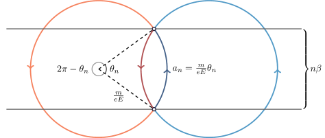
Figure 1: The four basic finite-temperature classical paths in the $x_{3}-x_{4}$ plane with a winding of $\pm n$ in the timelike direction, shown as portions of zero-temperature circular paths. All four paths begin and end on the same two points, which are separated by $n\beta$ in Euclidean time. From left to right, the paths are an antiparticle long path, an antiparticle short path, a particle short path and a particle long path. The radius $R$ is $m/eE$ and the length of the short arcs $a_{n}$ is $R\theta_{n}$.

In order for such solutions to exist at all, the diameter of the $T=0$ solution must be greater than $n\beta$,

$$2R=\frac{2m}{eE}>n\beta.$$ (16)

In other words, the maximum value of $n$, $n_{max}$ is given by

$$n_{max}=\left\lfloor\frac{2mT}{eE}\right\rfloor.$$ (17)

This implies that there are no one-loop thermal effects from worldline instantons for $T<eE/2m$, i.e., at sufficiently low temperatures Gies (2000).

Such solutions can be extended by adding on $p$ windings. The actions of these solutions are given by

$$S_{np}^{\left(s\right)} =\frac{m^{2}}{2eE}\left[\left(\theta_{n}+2\pi p\right)+\sin\theta_{n}\right]$$ (18)

$$S_{np}^{\left(l\right)} =\frac{m^{2}}{2eE}\left[\left(2\pi-\theta_{n}+2\pi p\right)-\sin\theta_{n}\right].$$ (19)

Note that

$$S_{np}^{\left(s\right)} =S_{n0}^{\left(s\right)}+S_{0p}$$ (20)

$$S_{np}^{\left(l\right)} =S_{n0}^{\left(l\right)}+S_{0p}$$ (21)

and that the two solutions become degenerate when $\theta_{n}=\pi.$

III.1 Fluctuation prefactors

The prefactors $K_{np}^{(s)}$ and $K_{np}^{(l)}$ are given in terms of the functional determinant of the second variation operator, which is the sum of a local and a nonlocal term Affleck et al. (1982):

$$M_{\mu\nu}\equiv\left.\frac{\delta S_{\mathit{eff}}}{\delta x_{\nu}\left(u^{\prime}\right)\delta x_{\mu}\left(u\right)}\right|_{x_{\mathit{cl}}}\!=L_{\mu\nu}-\vartheta\frac{eE}{R^{2}}\left(x_{\mu}\left(u\right)-\bar{x}_{\mu}\right)\left(x_{\nu}\left(u^{\prime}\right)-\bar{x}_{\nu}\right)$$ (22)

where

$$L_{\mu\nu}=\left[-\frac{eE}{\vartheta}\delta_{\mu\nu}\frac{d^{2}}{du^{2}}+ieF_{\mu\nu}\frac{d}{du}\right]\delta\left(u-u^{\prime}\right)$$ (23)

and $\vartheta$ is the total angle spanned by the instanton solution, that is, $\vartheta=2\pi p+\theta_{n}$ for short paths and $\vartheta=2\pi\left(p+1\right)-\theta_{n}$ for long paths. For fluctuations about zero temperature solutions, the eigenvalue problem for $M_{\mu\nu}$ can be solved by inspection. For fluctuations about finite temperature solutions this is made difficult by the boundary conditions at the endpoints. Fortunately, the functional determinant may be computed without any explicit knowledge of the spectrum. The matrix determinant lemma Sylvester (1851) can be used to isolate the effect of the nonlocal term,

$$\det\vphantom{}^{\prime}\left[M_{\mu\nu}\right]=\det\vphantom{}^{\prime}\left[L_{\mu\nu}\right]\cdot\left[1-\vartheta\frac{eE}{R^{2}}\iint du\,du^{\prime}\,\left(x\left(u\right)-\bar{x}\right)_{\mu}\left(L^{-1}\right)_{\mu\nu}\left(x\left(u^{\prime}\right)-\bar{x}\right)_{\nu}\right]$$ (24)

and the local part of the functional determinant is computed using the method of Gel’fand and Yaglom Gelfand and Yaglom (1960); Levit and Smilansky (1977). Consider the following set of initial value problems ($\rho=1,2,3,4$):

$$L_{\mu\nu}\eta_{\nu}^{\left(\rho\right)} =0$$ (25)

$$\eta_{\nu}^{\left(\rho\right)}\left(0\right) =0$$ (26)

$$\dot{\eta}_{\nu}^{\left(\rho\right)}\left(0\right) =\delta_{\nu\rho}$$ (27)

Up to a phase, the local prefactor can be written

$$\left(N\det\vphantom{}^{\prime}\left[L_{\mu\nu}\right]\right)^{-1/2}=\frac{\left(eE\right)^{2}}{\left(2\pi\vartheta\right)^{2}}\sqrt{\frac{\det\left[\tilde{\eta}_{\mu}^{\left(\nu\right)}\left(1\right)\right]}{\det\left[\eta_{\mu}^{\left(\nu\right)}\left(1\right)\right]}}$$ (28)

where $N$ is a normalization factor and $\tilde{\eta}_{\mu}^{\left(\nu\right)}$ are the solutions of the corresponding free initial value problem, with $\tilde{L}_{\mu\nu}=-\frac{eE}{\vartheta}\frac{d^{2}}{du^{2}}\delta_{\mu\nu}$. It is then straightforward to show

$$\left(N\det\vphantom{}^{\prime}\left[L_{\mu\nu}\right]\right)^{-1/2}=(-1)^{p}\frac{\left(eE\right)^{2}}{\left(2\pi\vartheta\right)^{2}}\sqrt{\frac{\vartheta^{2}}{2\left(1-\cos\vartheta\right)}}.$$ (29)

As we will see in section IV.1, the overall phase $e^{i2\pi p/2}=(-1)^{p}$ is related to the Morse index of the classical path. Note that this quantity is manifestly real, which means any imaginary contribution must come from the nonlocal part.

To compute the nonlocal part we find the Green’s function directly, by solving the equation

$$L_{\mu\rho}G_{\rho\nu}\left(u-u^{\prime}\right)=\delta_{\mu\nu}\delta\left(u-u^{\prime}\right)$$ (30)

with Dirichlet boundary conditions. A lengthy but straightforward calculation gives, for the nontrivial components $G_{33}=G_{44}$ and $G_{43}=-G_{34}$,

$$G_{33} =\frac{1}{2eE}\left[-\sin\left(\vartheta|u-u^{\prime}|\right)+\sin\left(\vartheta u^{\prime}\right)+\sin\left(\vartheta u\right)-\frac{4\sin\left(\frac{\vartheta}{2}u\right)\sin\left(\frac{\vartheta}{2}u^{\prime}\right)\cos\left(\frac{\vartheta}{2}\left(u-u^{\prime}\right)\right)}{\tan\left(\frac{\vartheta}{2}\right)}\right]$$ (31)

$$G_{43} =\frac{1}{2eE}\left[\operatorname{sgn}\left(u-u^{\prime}\right)\left(\cos\left(\vartheta|u-u^{\prime}|\right)-1\right)+\cos\left(\vartheta u^{\prime}\right)-\cos\left(\vartheta u\right)-\frac{\sin\left(\vartheta\left(u-u^{\prime}\right)\right)+\sin\left(\vartheta u^{\prime}\right)-\sin\left(\vartheta u\right)}{\tan\left(\frac{\vartheta}{2}\right)}\right].$$ (32)

The nonlocal part of the determinant can now be computed directly:

$$\left[1-\vartheta\frac{eE}{R^{2}}\iint du\,du^{\prime}\,x_{\mu}\left(u\right)G_{\mu\nu}\left(u-u^{\prime}\right)x_{\nu}\left(u^{\prime}\right)\right]=\frac{\vartheta}{2}\cot\left(\frac{\vartheta}{2}\right)$$ (33)

Note that for long paths $\pi<\vartheta<2\pi$ (modulo $2\pi$), so the nonlocal part of the determinant is negative. Because of this, it is clear that it is the long paths that contribute to the imaginary part of the effective action.

The prefactor can now be assembled as before

$$\left(\int d^{4}x\right)\frac{\sqrt{2\pi/m}}{\left[\int_{0}^{1}du\,\dot{x}^{2}\right]^{1/4}}\left(\det\vphantom{}^{\prime}\left[\left.\frac{\delta S_{\mathit{eff}}}{\delta x_{\nu}\left(u^{\prime}\right)\delta x_{\mu}\left(u\right)}\right|_{x_{\mathit{cl}}}\right]\right)^{-1/2} =V_{3}\beta\frac{\left(eE\right)^{2}}{\left(2\pi\right)^{3/2}\left(nm\beta\right)^{1/2}\vartheta^{2}}\left[1-\left(\frac{n\beta eE}{2m}\right)^{2}\right]^{-1/4}.$$ (34)

For long paths, an extra factor of $\pm i/2$ should be included because the contribution to the imaginary part results from an integration over only one half of the Gaussian peak in the imaginary direction Coleman (1979). The sign depends on the way in which the analytic continuation is performed.

The functional determinant for the short paths is always positive, and the functional determinant for the long paths is always negative, in agreement with arguments given in section IV.1. The sum of the short path contributions represents the free energy density of the metastable phase, and is given by

$$f=-\sum_{p=0}^{\infty}\sum_{n=1}^{n_{\mathit{\mathit{max}}}}2K_{np}^{\left(s\right)}e^{-S_{np}^{\left(s\right)}}$$ (35)

where

$$K_{np}^{(s)} =\frac{(-1)^{p}\left(eE\right)^{2}}{\left(2\pi\right)^{3/2}\left(n\beta m\right)^{1/2}\left[2\pi p+2\sin^{-1}\left(\frac{n\beta eE}{2m}\right)\right]^{2}}\left[1-\left(\frac{n\beta eE}{2m}\right)^{2}\right]^{-1/4}$$ (36)

$$S_{np}^{(s)} =\frac{m^{2}}{2eE}\left[2\pi p+2\sin^{-1}\left(\frac{n\beta eE}{2m}\right)+\frac{n\beta eE}{m}\sqrt{1-\left(\frac{n\beta eE}{2m}\right)^{2}}\right].$$ (37)

In the limit $E\rightarrow 0$, equation (35) precisely reproduces the free energy of a free relativistic particle in the limit $\beta m\gg 1$. Compare the limiting form of equation (35) with the exact expression Meisinger and Ogilvie (2002a)

$$f=-\frac{m^{2}}{\pi^{2}\beta^{2}}\sum_{n=1}^{\infty}\frac{1}{n^{2}}K_{2}(n\beta m).$$ (38)

As $\beta\rightarrow\infty$ we have

$$f\sim-\sum_{n=1}^{\infty}2\frac{m^{3/2}}{(2\pi)^{3/2}(n\beta)^{5/2}}e^{-n\beta m}$$ (39)

which is the precise form of equation (35) as $E\rightarrow 0$.

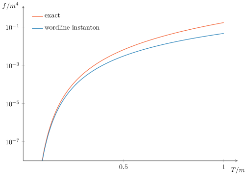
Figure 2: The worldline instanton expression for the free energy is an excellent approximation at low temperatures and $E\rightarrow 0$.

The long paths, on the other hand, give a thermal correction $\Gamma_{T}$ to the zero-temperature decay rate $\Gamma_{0}$. Our final result for scalars is

$$\Gamma_{T}=2\operatorname{Im}\left\{\sum_{p=0}^{\infty}\sum_{n=1}^{n_{\mathit{\mathit{max}}}}2K_{np}^{\left(l\right)}e^{-S_{np}^{\left(l\right)}}\right\}$$ (40)

where

$$K_{np}^{\left(l\right)} =\frac{i}{2}\cdot\frac{(-1)^{p}\left(eE\right)^{2}}{\left(2\pi\right)^{3/2}\left(n\beta m\right)^{1/2}\left[2\pi\left(p+1\right)-2\sin^{-1}\left(\frac{n\beta eE}{2m}\right)\right]^{2}}\left[1-\left(\frac{n\beta eE}{2m}\right)^{2}\right]^{-1/4}$$ (41)

$$S_{np}^{(s)} =\frac{m^{2}}{2eE}\left[2\pi\left(p+1\right)-2\sin^{-1}\left(\frac{n\beta eE}{2m}\right)-\frac{n\beta eE}{m}\sqrt{1-\left(\frac{n\beta eE}{2m}\right)^{2}}\right].$$ (42)

This concludes the derivation of our results for scalars in an external electric field.

IV Discussion

In this section, we discuss some of the unusual features of our results, and their generalization to related problems. In Fig. 6 we plot the total decay rate $\Gamma=\Gamma_{0}+\Gamma_{T}$ as a function of $T/m$ for three values of $eE/m^{2}.$ The leftmost part of each curve represents the contribution of $\Gamma_{0}$ alone, which is independent of temperature. Each curve shows singularities at $T/m=neE/2m^{2}$, indicated by dotted lines. Each singularity occurs at a threshold temperature above which a new worldline instanton solution becomes possible. It can be shown that, wherever it is nonzero, $\Gamma_{T}$ is always larger than $\Gamma_{0}$. By examining the reliable values of $\Gamma/m^{4}$ to the left of each singularity, we see that the overall rise in the decay rate envelope appears to be linear in $T$.

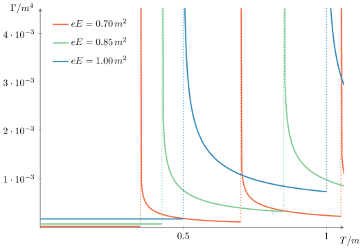
Figure 3: The total one-loop decay rate $\Gamma=\Gamma_{0}+\Gamma_{T}$ divided by $m^{4}$ versus $T/m$ for various values of $eE/m^{2}.$ The dotted lines represent the singularities at $T/m=neE/2m^{2}$, which are rendered finite by effects not included at one loop. The leftmost part of each curve represents the contribution of $\Gamma_{0}$ alone.

The set of thresholds is controlled by the dimensionless parameter $2mT/eE$, and by the associated integer part $n_{max}$. Any finite temperature instanton must satisfy $2R=2m/eE>n\beta$. If $n_{max}=0$, i.e. $T<eE/2m$, there are no finite temperature instantons, and therefore no corrections to the zero-temperature decay rate. As $T$ is increased, the threshold for a new solution is crossed whenever $n_{max}$ increases by one. This has some similarity with the problem of vacuum decay at finite temperature. In the problem of the decay of the false vacuum, the Euclidean bounce solution in the thin wall approximation is a critical bubble of radius $R_{c}$, obtained from the competition between volume and surface tension contributions to the bounce action. At nonzero temperature, this solution is unmodified until $2R_{c}>\beta$, that is, until the bubble diameter exceeds the length of the compact direction  Linde (1983); Garriga (1994). There are also some similarities with the problem of one-loop stability of gauge fields at finite temperature in an external field, but the mechanism there is different, and results from the competition between positive contributions to the energy eigenvalues from Matsubara frequencies with the negative contribution from the lowest Landau level Meisinger and Ogilvie (2002b).

IV.1 Morse-theoretic analysis

One of the striking features of our result for the decay rate, associated with the behavior at thresholds, is the singular behavior of the decay rate $\Gamma_{T}$. This singularity is due to the factor

$$\left[1-\left(\frac{n\beta eE}{2m}\right)^{2}\right]^{-1/4}$$ (43)

in eqns. (36) and (41) for the fluctuation prefactors $K_{np}^{(s)}$ and $K_{np}^{(l)}$. The origin of the singularity can be understood at the classical level, however. In Figure 4, we plot $S$ as a function of the angle $\theta$ for a family of paths with $n\beta m=1$ and fixed endpoint separation of $n\beta\hat{e}_{4}$. Classical solutions are only obtained at the extrema, where $R=m/eE$, and are given by $S_{n0}^{(s)}$ and $S_{n0}^{(l)}$. We see that for $eE/m^{2}<2$, there is a local minimum corresponding to the short path, and a local maximum corresponding to the long path. The instability of the long path is obvious. At $eE/m^{2}=2$, the two extrema merge and $n_{max}$ changes by one. The long and short paths are local maxima and minima of the action, respectively, along a given direction in functional space. Recall that $n_{max}$ is the greatest integer less than $2R/\beta=2mT/eE$. When $2mT/eE$ is an integer, the long and short paths are degenerate, and both are arcs of angle $\pi$ and arc length $\pi R$. If $T$ is increased slightly, the degeneracy is lifted and a new maximum and minimum of the action exist. The singularity in $K_{np}^{(s)}$ and $K_{np}^{(l)}$ is associated with the degeneracy of the two solutions. This behavior is reminiscent of the behavior associated with the classical spinodal, where a local maximum and minimum merge and the quadratic approximation fails.

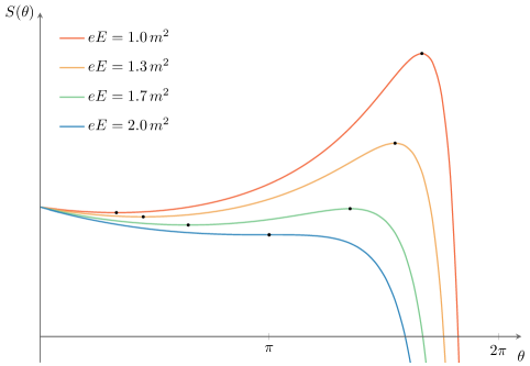
Figure 4: The action $S$ for an arc solution as a function of $\theta$ with $n\beta m=1$. Only the extrema, indicated by dots, represent classical solutions, with the short path solution a local minimum and the long path solution a local maximum. The values of the action at the extrema are given by $S_{n0}^{(s)}$ and $S_{n0}^{(l)}$, respectively. At $eE/m^{2}=2$, the two extrema merge.

This behavior is not restricted to the case of a constant, homogeneous electric field, but will occur generally for an inhomogeneous electric field when the temperature is nonzero and a zero-temperature instanton exists.

Morse theory provides a useful characterization of the eigenvalues of second variation operators about a functional extremum  Morse (1934); Levit and Smilansky (1977). The caustic is the envelope of trajectories obtained by fixing $x_{\mu}(0)$ and varying $\dot{x}_{\mu}(0)$. A focal point of a classical path is defined as a contact point between the path and the caustic surface. The central point of Morse theory may be stated thus: the number of negative eigenvalues of the second variation operator about a given classical path equals the number of focal points strictly between its endpoints, where each focal point is counted with its multiplicity. This number is the Morse index of the path.

In the present case, all classical solutions are circles of constant radius $R=m/eE$. Therefore, the caustic is the union of a larger circle of radius $2R$ with a single point at $x_{\mu}(0)$. A diagram illustrating this caustic is in figure 5. Zero-temperature wordline instanton solutions of winding $p$ (as well as our long paths of the same winding) contact the caustic $2p+1$ times, which establishes their imaginary contribution to the effective action. Short paths of winding $p$ contact the caustic $2p$ times, which nets a real contribution to the effective action. In either case, the $2p$ negative eigenvalues associated with additional windings result in an overall factor of $(-1)^{p}$ in the prefactor, as shown in equation (29). The appearance of such pairs of negative eigenvalues can be seen explicitly in the derivation of the functional determinant prefactor for zero-temperature solutions (see Appendix A).

We emphasize that these features do not depend on the exact shape of the wordline instanton solution. Exact worldline instanton trajectories are known for several inhomogeneous field configurations. These trajectories are no longer circles, but they are still closed and periodic Dunne et al. (2006). This is sufficient to establish that the striking qualitative features of our results – the singularities and thresholds, as well as the fact that short paths contribute to the free energy while long paths contribute the decay rate – are expected for inhomogeneous field configurations as well.

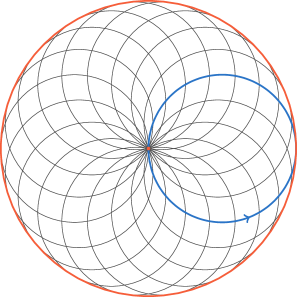
Figure 5: A set of trajectories formed by varying $\dot{x}(0)$. The envelope of such trajectories is the caustic, indicated in red. A representative path is in blue. As the path touches the caustic, the fluctuation operator about it acquires a negative eigenvalue.

IV.2 Higher order effects

We have seen in previous sections that the singularities in the effective action result from the inadequacy of the Gaussian approximation at points in functional space where two critical points become degenerate. At such points the quadratic coefficient in the Hessian operator vanishes and higher order terms are necessary for a correct computation of the effective action. The inclusion of such higher-order effects is difficult even at zero temperature. At finite temperature, higher-order effects will give rise to finite lifetimes for quasiparticle excitations in the thermal medium. These lifetimes may be calculated within the hard thermal loop (HTL) framework Braaten and Pisarski (1992). It is at least plausible that these finite lifetime effects smear out the threshold singularities, rendering the decay rate finite. A complete calculation of this type is far beyond our grasp. However, the singularities can be eliminated heuristically by including the effect of a damping rate for the charged scalars. A damping rate for scalar QED can be obtained from a hard-thermal-loop calculation of the imaginary part of the scalar self energy. We include this effect by replacing $m\rightarrow m-i\gamma$ in equation (43), where $\gamma\sim 0.04\,e^{2}T$ is the scalar damping rate Thoma and Traxler (1996); Abada and Bouakaz (2006). This amounts to replacing the singular factor

$$\left[1-\left(\frac{n\beta eE}{2m}\right)^{2}\right]^{-1/4}\rightarrow\left[\frac{1-\left(\frac{n\beta eE}{2m}\right)^{2}}{\Big{(}1-\left(\frac{n\beta eE}{2m}\right)^{2}\Big{)}^{2}+\Big{(}\frac{2\gamma}{m}\Big{(}\frac{n\beta eE}{2m}\Big{)}^{2}\Big{)}^{2}}\right]^{1/4}$$ (44)

in equation (41).

In Fig. 6 we plot the total decay rate $\Gamma=\Gamma_{0}+\Gamma_{T}$ as a function of $T/m$ with the modified threshold behavior for the same three values of $eE/m^{2}$ used in Fig. 6. As in that figure, the leftmost part of each curve represents the contribution of $\Gamma_{0}$ alone, which is independent of temperature. Each curve shows local maxima at $T/m=neE/2m^{2}$. There is very little difference between the unmodified and modified decay rates, except in the close vicinity of a threshold. We have tried other modifications of the decay rate using the HTL damping rate. the results are not sensitive to the particular modification used, and the decay rate away from thresholds is virtually unchanged. This indicates that the thermal contribution to the pair production is substantially larger than the $T=0$ contribution once the first threshold is crossed.

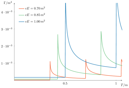
Figure 6: The total one-loop decay rate $\Gamma=\Gamma_{0}+\Gamma_{T}$ divided by $m^{4}$ versus $T/m$ for various values of $eE/m^{2}$, including HTL damping effects. The leftmost part of each curve represents the contribution of $\Gamma_{0}$ alone.

V Conclusions

We have presented a first-principles worldline instanton method for calculating the thermal contributions to Schwinger pair production in an electric field, and argued that many of the features will carry over to the case of inhomogeneous fields as well. While the worldline formalism is powerful, it is physically opaque. In Appendix B, we give a formal derivation of our results by applying a saddle-point approximation to the standard proper time representation of the effective potential for scalar bosons in an external electric field. A simple physical understanding of these results analogous to the many physically transparent derivations of the zero temperature decay rate would also be highly desirable.

The decay rate shows unphysical behavior at a series of thresholds, but this is an artifact of the Gaussian approximation to the functional integral; we have shown that this behavior is made physical by the phenomenological inclusion of hard thermal loop effects. Once the first threshold for thermal effects is crossed, the thermal contribution is larger than the the $T=0$ contribution, rising as each successive threshold is crossed. This strongly indicates the potential importance of thermal effects in all such nonperturbative pair production processes. We plan to extend this work to cases of more phenomenological interest, such as quarks in constant non-Abelian electric fields with Polyakov loop effects included.

After the completion of this work, a paper appeared on arXiv Brown (2015) that considers the same problem and has some overlap with our work. However, there is significant disagreement between our results.

Appendix A Fluctuation prefactor for zero temperature solution

First we illustrate the use of the matrix determinant lemma by computing the prefactor for the zero temperature worldline solutions. Because the local part $L_{\mu\nu}$ of the second variation operator (23) has zero modes associated with proper time translations and expansions/contractions of the zero temperature circle, it is noninvertible, which means the spectrum must be known and there is no benefit over the direct calculation. However, at finite temperature both zero modes are lifted and the method becomes much more convenient. The second variation of the action about the worldline instanton solution (assumed without loss of generality to be centered at the origin) is Affleck et al. (1982)

$$\left.\frac{\delta S_{\mathit{eff}}}{\delta x_{\nu}\left(u^{\prime}\right)\delta x_{\mu}\left(u\right)}\right|_{x_{\mathit{cl}}}=\left[-\frac{eE}{2\pi p}\frac{d^{2}}{du^{2}}\delta_{\mu\nu}+ieF_{\mu\nu}\frac{d}{du}\right]\delta\left(u-u^{\prime}\right)-2\pi p\frac{eE}{R^{2}}x_{\mu}\left(u\right)x_{\nu}\left(u^{\prime}\right).$$ (45)

The determinant can be written as

$$\det\vphantom{}^{\prime}\left[\left.\frac{\delta S_{\mathit{eff}}}{\delta x_{\nu}\left(u^{\prime}\right)\delta x_{\mu}\left(u\right)}\right|_{x_{\mathit{cl}}}\right] =\det\vphantom{}^{\prime}\left[L_{\mu\nu}\right]\left(1-2\pi p\frac{eE}{R^{2}}\iint du\,du^{\prime}\,x_{\mu}\left(u\right)\left(L{}^{-1}\right)^{\prime}_{\mu\nu}x_{\nu}\left(u^{\prime}\right)\right)\left(-2\pi peE\right)$$ (46)

$$L_{\mu\nu} =\left[-\frac{eE}{2\pi p}\frac{d^{2}}{du^{2}}\delta_{\mu\nu}+ieF_{\mu\nu}\frac{d}{du}\right].$$ (47)

As usual, the primed determinant and Green’s function are computed with zero modes removed. The last factor appears because, although changing the radius of the instanton circle is a zero mode of the local part, it is not a zero mode of the full second variation operator. The corresponding eigenvalue must be handled separately.

The determinant of the local part can be computed by enumerating eigenvalues, as in Affleck et al. Ignoring the irrelevant transverse directions we have

$$\det\vphantom{}^{\prime}\left[L_{\mu\nu}\right]=N\prod_{\begin{subarray}{c}q\neq 0\\ q\neq p\end{subarray}}\left(2\pi eE\left(\frac{q^{2}}{p}-q\right)\right)^{2}$$ (48)

where $N$ is a normalization factor to be fixed by the identity

$$\int_{x(1)=x(0)=\bar{x}}\left[dx\right]\exp\left[-\frac{m^{2}}{4s_{0}}\int_{0}^{1}du\,\dot{x}^{2}\right]=\left[N\det\vphantom{}^{\prime}\left(-\frac{m^{2}}{4s_{0}}\frac{d^{2}}{du^{2}}\right)\right]^{-1/2}=\frac{m^{4}}{\left(4\pi s_{0}\right)^{2}}.$$ (49)

Therefore,

$$\det\vphantom{}^{\prime}\left[L_{\mu\nu}\right] =\left(\frac{4\pi s_{0}}{m^{2}}\right)^{4}\frac{1}{\left(2\pi peE\right)^{2}}\prod_{\begin{subarray}{c}q\neq 0\\ q\neq p\end{subarray}}\frac{\left(\frac{q^{2}}{p}-q\right)^{2}}{\left(\frac{q^{2}}{p}\right)^{2}}$$ (50)

$$=\left(\frac{4\pi^{2}p}{eE}\right)^{4}\frac{1}{\left(2\pi peE\right)^{2}}\left[\lim_{z\rightarrow 1}\frac{\sin\left(\pi pz\right)}{\pi pz\left(1-z\right)}\right]^{2}$$ (51)

$$=\left[\left(\frac{4\pi^{2}p}{eE}\right)^{2}\frac{\left(-1\right)^{p+1}}{2\pi peE}\right]^{2}.$$ (52)

The second line comes from a standard identity Gradshteyn et al. (2007).

We now proceed to the nonlocal part which, as we will see, is trivial. The Green’s function $\left(L{}^{-1}\right)^{\prime}_{\mu\nu}$ can be obtained from the spectral representation

$$\left(L{}^{-1}\right)^{\prime}_{\mu\nu}=\sum_{\begin{subarray}{c}q\neq 0\\ q\neq p\end{subarray}}\frac{1}{\lambda_{q}}\left(\begin{array}[]{cc}\cos\left(2\pi q\left(u-u^{\prime}\right)\right)&-\sin\left(2\pi q\left(u-u^{\prime}\right)\right)\\ \sin\left(2\pi q\left(u-u^{\prime}\right)\right)&\cos\left(2\pi q\left(u-u^{\prime}\right)\right)\end{array}\right)$$ (53)

and thus

$$\int_{0}^{1}du\int_{0}^{1}du^{\prime}\,x_{\mu}\left(u\right)\left(L{}^{-1}\right)^{\prime}_{\mu\nu}x_{\nu}\left(u^{\prime}\right)=\sum_{\begin{subarray}{c}q\neq 0\\ q\neq p\end{subarray}}\frac{1}{\lambda_{q}}\left(\frac{\sin\left(\pi\left(p-q\right)\right)}{\pi\left(p-q\right)}\right)^{2}=0.$$ (54)

The last remaining piece to be evaluated is the contribution of the zero mode associated with proper time translations $x^{\mu}\left(2\pi pu\right)\rightarrow x^{\mu}\left(2\pi pu+\varphi\right)$. As usual, one need only consider an infinitesimal translation

$$x^{\mu}\left(2\pi pu+\varphi\right)\approx x^{\mu}\left(2\pi pu\right)+\varphi\left.\frac{d}{d\varphi}x^{\mu}\left(2\pi pu+\varphi\right)\right|_{\varphi=0}$$ (55)

and write the second term in terms of normalized eigenfunctions. Per this standard argument, a factor of

$$R\int_{0}^{2\pi}\frac{d\varphi}{\sqrt{2\pi}}=\sqrt{2\pi}\frac{m}{eE}$$ (56)

must be included in the functional integral.

Collecting everything, we obtain for the prefactor

$$\left(\int d^{4}x\right)\frac{\sqrt{2\pi/m}}{\left[\int_{0}^{1}du\,\dot{x}^{2}\right]^{1/4}}\left(\det\vphantom{}^{\prime}\left[\left.\frac{\delta S_{\mathit{eff}}}{\delta x_{\nu}\left(u^{\prime}\right)\delta x_{\mu}\left(u\right)}\right|_{x_{\mathit{cl}}}\right]\right)^{-1/2} =\pm V_{4}\frac{i}{2}\frac{\left(eE\right)^{2}}{\left(2\pi\right)^{3}p^{2}}\left(-1\right)^{p+1}$$ (57)

in agreement with Schwinger’s formula. The factor of $1/2$ comes from integrating over only one half of the Gaussian peak in the imaginary direction, and the sign depends on the way in which the analytic continuation is performed.

Appendix B Formal equivalence with proper time formalism

The proper time expression for the one-loop finite temperature contribution to the effective action of a charged scalar is Gies (1999)

$$\mathcal{L}^{1T}=-\frac{(eE)^{2}}{8\pi^{2}}\sum_{n=1}^{\infty}{\int_{0}^{\infty}{\frac{ds}{s^{2}}\csc(s)e^{-\frac{m^{2}}{eE}s-\frac{eE(n\beta)^{2}}{4}\cot(s)}}}.$$ (58)

We wish to calculate a Gaussian approximation to this integral. The exponent has pairs of saddle points given implicitly by

$$\sin(s_{0})=\frac{n\beta eE}{2m}\equiv\frac{n\beta}{2R}$$ (59)

provided the right side is smaller than $1$, that is, $n\leq n_{\mathit{max}}$ (see eq. (17)). For definiteness and simplicity we take $s_{0}$ to lie in the first quadrant, corresponding to our short path solutions. The second derivative of the exponent at the saddle point is

$$\left.\frac{\partial^{2}}{\partial s^{2}}\left(\frac{m^{2}}{eE}s+\frac{eE(n\beta)^{2}}{4}\cot(s)\right)\right|_{s_{0}}=\frac{eE(n\beta)^{2}}{2}\cot(s_{0})\csc^{2}(s_{0})=\frac{4m^{3}}{(eE)^{2}(n\beta)}\sqrt{1-\left(\frac{n\beta}{2R}\right)^{2}}.$$ (60)

The Gaussian approximation to the integral reads

$$\mathcal{L}_{(n)}^{1T} =-\frac{\left(eE\right){}^{2}}{8\pi^{2}}\sum_{n=1}^{n_{\mathit{max}}}\frac{1}{s_{0}^{2}}\frac{2R}{n\beta}\left(2\pi\frac{(eE)^{2}n\beta}{4m^{3}\sqrt{1-(\frac{n\beta}{2R})^{2}}}\right)^{1/2}e^{-S(s_{0})}$$ (61)

$$=-\frac{(eE)^{2}}{\sqrt{2\pi^{3}}}\sum_{n=1}^{n_{\mathit{max}}}\sum_{p=0}^{\infty}\frac{1}{\left(nm\beta\right)^{1/2}\left(2\pi p+2\sin^{-1}\left(\frac{n\beta eE}{2m}\right)\right)^{2}}\left[1-\left(\frac{n\beta eE}{2m}\right)^{2}\right]^{-1/4}e^{-S(s_{0})}$$ (62)

where

$$S\left(s_{0}\right)=\frac{m^{2}}{2eE}\left[2\pi p+2\sin^{-1}\left(\frac{n\beta eE}{2m}\right)+\frac{n\beta eE}{m}\sqrt{1-\left(\frac{n\beta eE}{2m}\right)^{2}}\right]$$ (63)

in complete agreement with equations (35) and (36).

References

- Parker (1969) L. Parker, Phys. Rev. 183, 1057 (1969).
- Zeldovich and Starobinsky (1972) Ya. B. Zeldovich and A. A. Starobinsky, Sov. Phys. JETP 34, 1159 (1972), [Zh. Eksp. Teor. Fiz.61,2161(1971)].
- Hawking (1974) S. W. Hawking, Nature 248, 30 (1974).
- Casher et al. (1979) A. Casher, H. Neuberger, and S. Nussinov, Phys. Rev. D20, 179 (1979).
- Ringwald (2001) A. Ringwald, in Electromagnetic probes of fundamental physics. Proceedings, Workshop, Erice, Italy, October 16-21, 2001 (2001) pp. 63–74, arXiv:hep-ph/0112254 [hep-ph] .
- Kharzeev and Tuchin (2005) D. Kharzeev and K. Tuchin, Nucl. Phys. A753, 316 (2005), arXiv:hep-ph/0501234 [hep-ph] .
- Heisenberg and Euler (1936) W. Heisenberg and H. Euler, Z. Phys. 98, 714 (1936), arXiv:physics/0605038 [physics] .
- Schwinger (1951) J. S. Schwinger, Phys. Rev. 82, 664 (1951).
- Langer (1967) J. S. Langer, Annals Phys. 41, 108 (1967), [Annals Phys.281,941(2000)].
- Coleman (1977) S. R. Coleman, Phys. Rev. D15, 2929 (1977), [Erratum: Phys. Rev.D16,1248(1977)].
- Callan and Coleman (1977) C. G. Callan, Jr. and S. R. Coleman, Phys. Rev. D16, 1762 (1977).
- Affleck et al. (1982) I. K. Affleck, O. Alvarez, and N. S. Manton, Nucl. Phys. B197, 509 (1982).
- Affleck (1981) I. Affleck, Phys. Rev. Lett. 46, 388 (1981).
- Brezin and Itzykson (1970) E. Brezin and C. Itzykson, Phys. Rev. D2, 1191 (1970).
- Popov and Marinov (1972) V. S. Popov and M. S. Marinov, Yad. Fiz. 16, 809 (1972).
- Marinov and Popov (1977) M. S. Marinov and V. S. Popov, Fortsch. Phys. 25, 373 (1977).
- Dunne (2004) G. V. Dunne, Heisenberg-Euler effective Lagrangians: Basics and extensions (2004) arXiv:hep-th/0406216 [hep-th] .
- Gies and Klingmuller (2005) H. Gies and K. Klingmuller, Phys. Rev. D72, 065001 (2005), arXiv:hep-ph/0505099 [hep-ph] .
- Dunne and Schubert (2005) G. V. Dunne and C. Schubert, Phys. Rev. D72, 105004 (2005), arXiv:hep-th/0507174 [hep-th] .
- Dunne et al. (2006) G. V. Dunne, Q.-h. Wang, H. Gies, and C. Schubert, Phys. Rev. D73, 065028 (2006), arXiv:hep-th/0602176 [hep-th] .
- Dunne (2012) G. V. Dunne, Proceedings, 10th Conference on Quantum field theory under the influence of external conditions (QFEXT 11), Int. J. Mod. Phys. A27, 1260004 (2012), [Int. J. Mod. Phys. Conf. Ser.14,42(2012)], arXiv:1202.1557 [hep-th] .
- Dittrich (1979) W. Dittrich, Phys. Rev. D19, 2385 (1979).
- Elmfors et al. (1993) P. Elmfors, D. Persson, and B.-S. Skagerstam, Phys. Rev. Lett. 71, 480 (1993), arXiv:hep-th/9305004 [hep-th] .
- Loewe and Rojas (1992) M. Loewe and J. C. Rojas, Phys. Rev. D46, 2689 (1992).
- Elmfors and Skagerstam (1995) P. Elmfors and B.-S. Skagerstam, Phys. Lett. B348, 141 (1995), [Erratum: Phys. Lett.B376,330(1996)], arXiv:hep-th/9404106 [hep-th] .
- Hallin and Liljenberg (1995) J. Hallin and P. Liljenberg, Phys. Rev. D52, 1150 (1995), arXiv:hep-th/9412188 [hep-th] .
- Ganguly et al. (1995) A. K. Ganguly, J. C. Parikh, and P. K. Kaw, Phys. Rev. C51, 2091 (1995).
- Ganguly (1998) A. K. Ganguly, (1998), arXiv:hep-th/9804134 [hep-th] .
- Gies (1999) H. Gies, Phys. Rev. D60, 105002 (1999), arXiv:hep-ph/9812436 [hep-ph] .
- Gies (2000) H. Gies, Phys. Rev. D61, 085021 (2000), arXiv:hep-ph/9909500 [hep-ph] .
- Bern and Kosower (1992) Z. Bern and D. A. Kosower, Nucl. Phys. B379, 451 (1992).
- Strassler (1992) M. J. Strassler, Nucl. Phys. B385, 145 (1992), arXiv:hep-ph/9205205 [hep-ph] .
- Schubert (2001) C. Schubert, Phys. Rept. 355, 73 (2001), arXiv:hep-th/0101036 [hep-th] .
- Andersson et al. (1983) B. Andersson, G. Gustafson, G. Ingelman, and T. Sjostrand, Phys. Rept. 97, 31 (1983).
- Bass et al. (1998) S. A. Bass et al., Prog. Part. Nucl. Phys. 41, 255 (1998), [Prog. Part. Nucl. Phys.41,225(1998)], arXiv:nucl-th/9803035 [nucl-th] .
- Coleman (1988) S. R. Coleman, Nucl. Phys. B298, 178 (1988).
- Liang and Muller-Kirsten (1994) J. Q. Liang and H. J. W. Muller-Kirsten, Phys. Rev. D50, 6519 (1994).
- Battarra et al. (2012) L. Battarra, G. Lavrelashvili, and J.-L. Lehners, Phys. Rev. D86, 124001 (2012), arXiv:1208.2182 [hep-th] .
- McKeon and Rebhan (1993) D. G. C. McKeon and A. Rebhan, Phys. Rev. D47, 5487 (1993), arXiv:hep-th/9211076 [hep-th] .
- Shovkovy (1998) I. A. Shovkovy, Phys. Lett. B441, 313 (1998), arXiv:hep-th/9806156 [hep-th] .
- Sylvester (1851) J. J. Sylvester, Philosophical Magazine 1, 295 (1851).
- Gelfand and Yaglom (1960) I. M. Gelfand and A. M. Yaglom, J. Math. Phys. 1, 48 (1960).
- Levit and Smilansky (1977) S. Levit and U. Smilansky, Annals Phys. 103, 198 (1977).
- Coleman (1979) S. R. Coleman, 15th Erice School of Subnuclear Physics: The Why’s of Subnuclear Physics Erice, Italy, July 23-August 10, 1977, Subnucl. Ser. 15, 805 (1979).
- Meisinger and Ogilvie (2002a) P. N. Meisinger and M. C. Ogilvie, Phys. Rev. D65, 056013 (2002a), arXiv:hep-ph/0108026 [hep-ph] .
- Linde (1983) A. D. Linde, Nucl. Phys. B216, 421 (1983), [Erratum: Nucl. Phys.B223,544(1983)].
- Garriga (1994) J. Garriga, Phys. Rev. D49, 5497 (1994), arXiv:hep-th/9401020 [hep-th] .
- Meisinger and Ogilvie (2002b) P. N. Meisinger and M. C. Ogilvie, Phys. Rev. D66, 105006 (2002b), arXiv:hep-ph/0206181 [hep-ph] .
- Morse (1934) M. Morse, The Calculus of Variations in the Large, American Mathematical Society No. v. 18 (American mathematical society, 1934).
- Braaten and Pisarski (1992) E. Braaten and R. D. Pisarski, Phys. Rev. D46, 1829 (1992).
- Thoma and Traxler (1996) M. H. Thoma and C. T. Traxler, Phys. Lett. B378, 233 (1996), arXiv:hep-ph/9601254 [hep-ph] .
- Abada and Bouakaz (2006) A. Abada and K. Bouakaz, JHEP 01, 161 (2006), arXiv:hep-ph/0510330 [hep-ph] .
- Brown (2015) A. R. Brown, (2015), arXiv:1512.05716 [hep-th] .
- Gradshteyn et al. (2007) I. S. Gradshteyn, I. M. Ryzhik, A. Jeffrey, D. Zwillinger, and I. Scripta Technica, Table of integrals, series, and products (Elsevier, Amsterdam, Boston, Paris, et al., 2007) trad. de : Tabli?t?sy integralov, summ, r?i?adov i proizvedeni?