SNAP: Stateful Network-Wide
Abstractions for Packet Processing

Abstract

Early programming languages for software-defined networking (SDN) were built on top of the simple match-action paradigm offered by OpenFlow 1.0. However, emerging hardware and software switches offer much more sophisticated support for persistent state in the data plane, without involving a central controller. Nevertheless, managing stateful, distributed systems efficiently and correctly is known to be one of the most challenging programming problems. To simplify this new SDN problem, we introduce SNAP.

SNAP offers a simpler “centralized” stateful programming model, by allowing programmers to develop programs on top of one big switch rather than many. These programs may contain reads and writes to global, persistent arrays, and as a result, programmers can implement a broad range of applications, from stateful firewalls to fine-grained traffic monitoring. The SNAP compiler relieves programmers of having to worry about how to distribute, place, and optimize access to these stateful arrays by doing it all for them. More specifically, the compiler discovers read/write dependencies between arrays and translates one-big-switch programs into an efficient internal representation based on a novel variant of binary decision diagrams. This internal representation is used to construct a mixed-integer linear program, which jointly optimizes the placement of state and the routing of traffic across the underlying physical topology. We have implemented a prototype compiler and applied it to about 20 SNAP programs over various topologies to demonstrate our techniques’ scalability.

<ccs2012> <concept> <concept_id>10003033.10003034.10003038</concept_id> <concept_desc>Networks Programming interfaces</concept_desc> <concept_significance>500</concept_significance> </concept> <concept> <concept_id>10003033.10003099.10003102</concept_id> <concept_desc>Networks Programmable networks</concept_desc> <concept_significance>500</concept_significance> </concept> <concept> <concept_id>10003033.10003068.10003073.10003075</concept_id> <concept_desc>Networks Network control algorithms</concept_desc> <concept_significance>300</concept_significance> </concept> <concept> <concept_id>10003033.10003099.10003103</concept_id> <concept_desc>Networks In-network processing</concept_desc> <concept_significance>300</concept_significance> </concept> <concept> <concept_id>10003033.10003099.10003104</concept_id> <concept_desc>Networks Network management</concept_desc> <concept_significance>300</concept_significance> </concept> </ccs2012>

[500]Networks Programming interfaces [500]Networks Programmable networks [300]Networks Network control algorithms [300]Networks In-network processing [300]Networks Network management

1 Introduction

The first generation of programming languages for software-defined networks (SDNs) [14, 10, 43, 20, 17] was built on top of OpenFlow 1.0, which offered simple match-action processing of packets. As a result, these systems were partitioned into (1) a stateless packet-processing part that could be analyzed statically, compiled, and installed on OpenFlow switches, and (2) a general stateful component that ran on the controller.

This “two-tiered” programming model can support any network functionality by running the stateful portions of the program on the controller and modifying the stateless packet-processing rules accordingly. However, simple stateful programs, such as detecting SYN floods or DNS amplification attacks, cannot be implemented efficiently because packets must go back-and-forth to the controller, incurring significant delay. Thus, in practice, stateful controller programs are limited to those that do not require per-packet stateful processing.

Today, however, SDN technology has advanced considerably: there is a raft of new proposals for switch interfaces that expose persistent state on the data plane, including those in P4 [6], OpenState [4], POF [38], Domino [33], and Open vSwitch [25]. Stateful programmable data planes enable us to offload programs that require per-packet stateful processing onto switches, subsuming a variety of functionality normally relegated to middleboxes. However, the mere existence of these stateful mechanisms does not make networks of these devices easy to program. In fact, programming distributed collections of stateful devices is typically one of the most difficult kinds of programming problems. We need new languages and abstractions to help us manage the complexity and optimize resource utilization effectively.

For these reasons, we have developed SNAP, a new language that allows programmers to mix primitive stateful operations with pure packet processing. However, rather than ask programmers to program a large, distributed collection of independent, stateful devices manually, we provide the abstraction that the network is one big switch (OBS). Programmers can allocate persistent arrays on that OBS , and do not have to worry about where or how such arrays are stored in the physical network. Such arrays can be indexed by fields in incoming packets and modified over time as network conditions change. Moreover, if multiple arrays must be updated simultaneously, we provide a form of network transaction to ensure such updates occur atomically. As a result, it is easy to write SNAP programs that learn about the network environment and record its state, store per-flow information or statistics, or implement a variety of stateful mechanisms.

While it simplifies programming, the OBS model, together with the stateful primitives, generates implementation challenges. In particular, multiple flows may depend upon the same state. To process these flows correctly and efficiently, the compiler must simultaneously determine which flows depend upon which components, how to route those flows, and where to place the components. Hence, to map OBS programs to concrete topologies, the SNAP compiler discovers read-write dependencies between statements. It then translates the program into an xFDD, a variant of forwarding decision diagrams (FDDs) [35] extended to incorporate stateful operations. Next, the compiler generates a system of integer-linear equations that jointly optimizes array placement and traffic routing. Finally, the compiler generates the switch-level configurations from the xFDD and the optimization results. We assume that the switches chosen for array placement support persistent programmable state; other switches can still play a role in routing flows efficiently through the state variables. Our main contributions are:

• A stateful and compositional SDN programming language with persistent global arrays, a one-big-switch programming model, and network transactions. (See §2 for an overview and §3 for more technical details.)

• Algorithms for compiling SNAP programs into low-level switch mechanisms (§4): (i) an algorithm for compiling SNAP programs into an intermediate representation that detects program errors, such as race conditions introduced by parallel access to stateful components, using our extended forwarding decision diagrams (xFDD) and (ii) an algorithm to generate a mixed integer-linear program, based on the xFDD, which jointly decides array placement and routing while minimizing network congestion and satisfying the constraints necessary for network transactions.

• An implementation and evaluation of our language and compiler using about 20 applications. (§5, §6).

We discuss various data-plane implementations for SNAP, how SNAP relates to middleboxes, and possible extensions in §7, discuss related work in §8, and conclude in §9.

2 SNAP System Overview

This section overviews the key concepts in our language and compilation process using example programs.

2.1 Writing SNAP Programs

DNS-tunnel-detect

if dstip = 10.0.6.0/24 & srcport = 53 then
     orphan[dstip][dns.rdata] <- True;
     susp-client[dstip]++;
     if susp-client[dstip] = threshold then
          blacklist[dstip] <- True
     else id
else
     if srcip = 10.0.6.0/24 & orphan[srcip][dstip]
     then orphan[srcip][dstip] <- False;
              susp-client[srcip]--
   else id

Figure 1: SNAP implementation of DNS-tunnel-detect.

DNS tunnel detection. The DNS protocol is designed to resolve information about domain names. Since it is not intended for general data transfer, DNS often draws less attention in terms of security monitoring than other protocols, and is used by attackers to bypass security policies and leak information. Detecting DNS tunnels is one of many real-world scenarios that require state to track the properties of network flows [5]. The following steps can be used to detect DNS tunneling [5]:

1. For each client, keep track of the IP addresses resolved by DNS responses.

2. For each DNS response, increment a counter. This counter tracks the number of resolved IP addresses that a client does not use.

3. When a client sends a packet to a resolved IP address, decrement the counter for the client.

4. Report tunneling for clients that exceed a threshold for resolved, but unused IP addresses.

Figure 1 shows a SNAP implementation of the above steps that detects DNS tunnels to/from the CS department subnet 10.0.6.0/24 (see Figure 2). Intuitively, a SNAP program can be thought of as a function that takes in a packet plus the current state of the network and produces a set of transformed packets as well as updated state. The incoming packet is read and written by referring to its fields (such as dstip and dns.rdata). The “state” of the network is read and written by referring to user-defined, array-based, global variables (such as orphan or susp-client). Before explaining the program in detail, note that it does not refer to specific network device(s) on which it is implemented. SNAP programs are expressed as if the network was one-big-switch (OBS) connecting edge ports directly to each other. Our compiler automatically distributes the program across network devices, freeing programmers from such details and making SNAP programs portable across topologies.

The DNS-tunnel-detect program examines two kinds of packets: incoming DNS responses (which may lead to possible DNS tunnels) and outgoing packets to resolved IP addresses. Line 1 checks whether the input packet is a DNS response to the CS department. The condition in the if statement is an example of a simple test. Such tests can involve any boolean combination of packet fields. If the test succeeds, the packet could potentially belong to a DNS tunnel, and will go through the detection steps (Lines 2–6). Lines 2–6 use three global variables to keep track of DNS queries. Each variable is a mapping between keys and values, persistent across multiple packets. The orphan variable, for example, maps each pair of IP addresses to a boolean value. If orphan[c][s] is True then c has received a DNS response for IP address s. The variable susp-client maps the client’s IP to the number of DNS responses it has received but not accessed yet. If the packet is not a DNS response, a different test is performed, which includes a stateful test over orphan (Lines 8). If the test succeeds, the program updates orphan[srcip][dstip] to False and decrements susp-client[srcip] (Lines 10–11). This step changes the global state and thus, affects the processing of future packets. Otherwise, the packet is left unmodified — id (Line 12) is a no-op.

Routing. DNS-tunnel-detect cannot stand on its own—it does not explain where to forward packets. In SNAP, we can easily compose it with a forwarding policy. Suppose our target network is the simplified campus topology depicted in Figure 2. Here, $I_{1}$ and $I_{2}$ are connections to the Internet, and $D_{1}$–$D_{4}$ represent edge switches in the departments, with $D_{4}$ connected to the CS building. $C_{1}$–$C_{6}$ are core routers connecting the edges. External ports (marked in red) are numbered 1–6 and IP subnet 10.0.i.0/24 is attached to port i. The assign-egress program assigns outports to packets based on their destination IP address: assign-egress = if dstip = 10.0.1.0/24
then outport <- 1
else if dstip = 10.0.2.0/24 then outport <- 2
else ...
else if dstip = 10.0.6.0/24 then outport <- 6
else drop

Note that the policy is independent of the internal network structure, and recompilation is needed only if the topology changes. By combining DNS-tunnel-detect with assign-egress, we have implemented a useful end-to-end program: DNS-tunnel-detect;assign-egress.

Monitoring. Suppose the operator wants to monitor packets entering the network at each ingress port (ports 1-6). She might use an array indexed by inport and increment the corresponding element on packet arrival: count[inport]++. Monitoring should take place alongside the rest of the program; thus, she might combine it using parallel composition (+): (DNS-tunnel-detect + count[inport]++); assign-egress. Intuitively, p + q makes a copy of the incoming packet and executes both p and q on it simultaneously.

Note that it is not always legal to compose two programs in parallel. For instance, if one writes to the same global variable that the other reads, there is a race condition, which leads to ambiguous state in the final program. Our compiler detects such race conditions and rejects ambiguous programs.

Network Transactions. Suppose that an operator sets up a honeypot at port 3 with IP subnet 10.0.3.0/25. The following program records, per inport, the IP and dstport of the last packet destined to the honeypot:

if dstip = 10.0.3.0/25
then hon-ip[inport] <- srcip;
         hon-dstport[inport] <- dstport
else id

Since this program processes many packets simultaneously, it has an implicit race condition: if packets $p_{1}$ and $p_{2}$, both destined to the honeypot, enter the network from port 1 and get reordered, each may visit hon-ip and hon-dstport in a different order (if the variables reside in different locations). Therefore, it is possible that hon-ip[1] contains the source IP of $p_{1}$ and hon-dstport[1] the destination port of $p_{2}$ while the operator’s intention was that both variables refer to the same packet. To establish such properties for a collection of state variables, programmers can use network transactions by simply enclosing a series of statements in an atomic block. Atomic blocks co-locate their enclosed state variables so that a series of updates can be made to appear atomic.

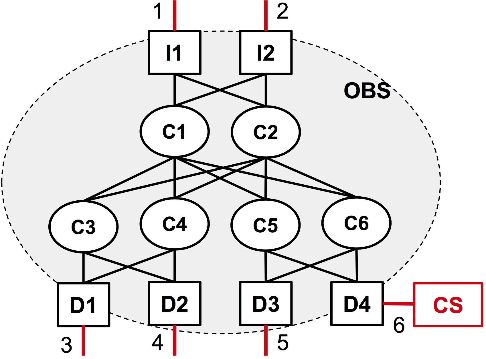
Figure 2: Topology for the running example.

2.2 Realizing Programs on the Data Plane

Consider DNS-tunnel-detect; assign-egress. To distribute this program across network devices, the SNAP compiler should decide (i) where to place state variables (orphan, susp-client, and blacklist), and (ii) how packets should be routed across the physical network. These decisions should be made in such a way that each packet passes through devices storing every state variable it needs, in the correct order. Therefore, the compiler needs information about which packets need which state variables. In our example program, for instance, packets with dstip = 10.0.6.0/24 and srcport = 53 need to pass all three state variables, with blacklist accessed after the other two.

Program analysis. To extract the above information, we transform the program to an intermediate representation called extended forwarding decision diagram (xFDD) (see Figure 3). FDDs were originally introduced in an earlier work [35]. We extended FDDs in SNAP to support stateful packet processing. An xFDD is like a binary decision diagram: each intermediate node is a test on either packet fields or state variables. The leaf nodes are sets of action sequences, rather than merely ‘true’ and ‘false’ as in a BDD [1]. Each interior node has two successors: true (solid line), which determines the rest of the forwarding decision process for inputs passing the test, and false (dashed line) for failed cases. xFDDs are constructed compositionally; the xFDDs for different parts of the program are combined to construct the final xFDD. Composition is particularly more involved with stateful operations: the same state variable may be referenced in two xFDDs with different header fields, e.g., once as s[srcip] and then as s[dstip]. How can we know whether or not those fields are equal in the packet? We add a new kind of test, over pairs of packet fields (srcip = dstip), and new ordering requirements on the xFDD structure.

Once the program is transformed to an xFDD, we analyze the xFDD to extract information about which groups of packets need which state variables. In Figure 3, for example, leaf number 10 is on the true branch of dstip=10.0.6.0/24 and srcport=53, which indicates that all packets with this property may end up there. These packets need orphan, because it is modified, and susp-client, because it is both tested and modified on the path. We can also deduce these packets can enter the network from any port and the ones that are not dropped will exit port 6. Thus, we can use the xFDD to figure out which packets need which state variables, aggregate this information across OBS ports, and choose paths for traffic between these ports accordingly.

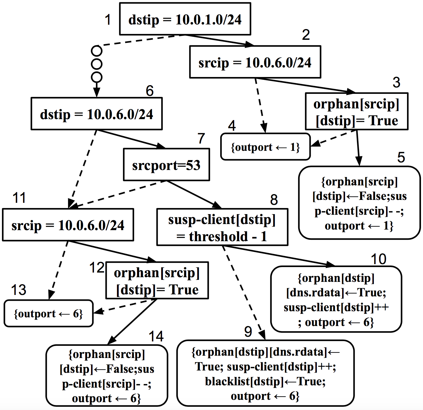
Figure 3: The equivalent xFDD for
DNS-tunnel-detect; assign-egress

Joint placement and routing. At this stage, the compiler has the information it needs to distribute the program. It uses a mixed-integer linear program (MILP) that solves an extension of the multi-commodity flow problem to jointly decide state placement and routing while minimizing network congestion. The constraints in the MILP guarantee that the selected paths for each pair of OBS ports take corresponding packets through devices storing every state variable that they need, in the correct order. Note that the xFDD analysis can identify cases in which both directions of a connection need the same state variable $s$, so the MILP ensures they both traverse the device holding $s$.

In our example program, the MILP places all state variables on D₄, which is the optimal location as all packets to and from the protected subnet must flow through D₄. Note that this is not obvious from the DNS-tunnel-detect code alone, but rather from its combination with assign-egress. This highlights the fact that in SNAP, program components can be written in a modular way, while the compiler makes globally optimal decisions using information from all parts. The optimizer also decides forwarding paths between external ports. For instance, traffic from $I_{1}$ and $D_{1}$ will go through $C_{1}$ and $C_{5}$ to reach $D_{4}$. The path from $I_{2}$ and $D_{2}$ to $D_{4}$ goes through $C_{2}$ and $C_{6}$, and $D_{3}$ uses $C_{5}$ to reach $D_{4}$. The paths between the rest of the ports are also determined by the MILP in a way that minimizes link utilization. The compiler takes state placement and routing results from the MILP, partitions the program’s intermediate representation (xFDD) among switches, and generates rules for the controller to push to all stateless and stateful switches in the network.

Reacting to network events. The above phases only run if the operator changes the OBS program. Once the program compiles, and to respond to network events such as failures or traffic shifts, we use a simpler and much faster version of the MILP that given the current state placement, only re-optimizes for routing. Moreover, with state on the data plane, policy changes become considerably less frequent because the policy, and consequently switch configurations, do not change upon changes to state. In DNS-tunnel-detect, for instance, attack detection and mitigation are both captured in the program itself, happen on the data plane, and therefore react rapidly to malicious activities in the network. This is in contrast to the case where all the state is on the controller. There, the policy needs to change and recompile multiple times both during detection and on mitigation, to reflect the state changes on the controller in the rules on the data plane.

3 SNAP

SNAP is a high-level language with two key features: programs are stateful and are written in terms of an abstract network topology comprising a one-big-switch (OBS). It has an algebraic structure patterned on the NetCore/NetKAT family of languages [19, 2], with each program comprising one or more predicates and policies. SNAP’s syntax is in Figure 4. Its semantics is defined through an evaluation function “$\mathsf{eval}{}$.” $\mathsf{eval}{}$ determines, in mathematical notation, how an input packet should be processed by a SNAP program. Note that this is part of the specification of the language, not the implementation. Any implementation of SNAP, including ours, should ensure that packets are processed as defined by the $\mathsf{eval}{}$ function: when we talk about “running” a program on a packet, we mean calling $\mathsf{eval}{}$ on that program and packet. We discuss $\mathsf{eval}{}$’s most interesting cases here; see appendix A for a full definition.

$\mathsf{eval}{}$ takes the SNAP term of interest, a packet, and a starting state and yields a set of packets and an output state. To properly define the semantics of multiple updates to state when programs are composed, we need to know the reads and writes to state variables performed by each program while evaluating the packet. Thus, $\mathsf{eval}{}$ also returns a log containing this information. It adds “$R\,s$” to the log whenever a read from state variable $s$ occurs, and “$W\,s$” on writes. Note that these logs are part of our formalism, but not our implementation. We express the program state as a dictionary that maps state variables to their contents. The contents of each state variable is itself a mapping from values to values. Values are defined as packet-related fields (IP address, TCP ports, MAC addresses, DNS domains) along with integers, booleans and vectors of such values.

$$\begin{array}[]{rcll}e\in\mathsf{Expr}&::=&v\,|\,f\,|\,\overset{\rightharpoonup}{e}&\\ x,y\in\mathsf{Pred}&::=&id&\text{Identity}\\ &|&drop&\text{Drop}\\ &|&f=v&\text{Test}\\ &|&\neg x&\text{Negation}\\ &|&x|y&\text{Disjunction}\\ &|&y\&x&\text{Conjunction}\\ &|&\mathchoice{{\hbox{\pagecolor{yellow}$\displaystyle s[e]=e$}}}{{\hbox{\pagecolor{yellow}$\textstyle s[e]=e$}}}{{\hbox{\pagecolor{yellow}$\scriptstyle s[e]=e$}}}{{\hbox{\pagecolor{yellow}$\scriptscriptstyle s[e]=e$}}}&\textbf{State Test}\\ p,q\in\mathsf{Pol}&::=&x&\text{Filter}\\ &|&f\leftarrow v&\text{Modification}\\ &|&p+q&\text{Parallel comp.}\\ &|&p;q&\text{Sequential comp.}\\ &|&\mathchoice{{\hbox{\pagecolor{yellow}$\displaystyle s[e]\leftarrow e$}}}{{\hbox{\pagecolor{yellow}$\textstyle s[e]\leftarrow e$}}}{{\hbox{\pagecolor{yellow}$\scriptstyle s[e]\leftarrow e$}}}{{\hbox{\pagecolor{yellow}$\scriptscriptstyle s[e]\leftarrow e$}}}&\textbf{State Modification}\\ &|&\mathchoice{{\hbox{\pagecolor{yellow}$\displaystyle s[e]\footnotesize\texttt{++}$}}}{{\hbox{\pagecolor{yellow}$\textstyle s[e]\footnotesize\texttt{++}$}}}{{\hbox{\pagecolor{yellow}$\scriptstyle s[e]\footnotesize\texttt{++}$}}}{{\hbox{\pagecolor{yellow}$\scriptscriptstyle s[e]\footnotesize\texttt{++}$}}}&\textbf{Increment value}\\ &|&\mathchoice{{\hbox{\pagecolor{yellow}$\displaystyle s[e]\text{\footnotesize{-{}-}}$}}}{{\hbox{\pagecolor{yellow}$\textstyle s[e]\text{\footnotesize{-{}-}}$}}}{{\hbox{\pagecolor{yellow}$\scriptstyle s[e]\text{\footnotesize{-{}-}}$}}}{{\hbox{\pagecolor{yellow}$\scriptscriptstyle s[e]\text{\footnotesize{-{}-}}$}}}&\textbf{Decrement value}\\ &|&\mathchoice{{\hbox{\pagecolor{yellow}$\displaystyle\text{if }a\text{ then }p\text{ else }q$}}}{{\hbox{\pagecolor{yellow}$\textstyle\text{if }a\text{ then }p\text{ else }q$}}}{{\hbox{\pagecolor{yellow}$\scriptstyle\text{if }a\text{ then }p\text{ else }q$}}}{{\hbox{\pagecolor{yellow}$\scriptscriptstyle\text{if }a\text{ then }p\text{ else }q$}}}&\textbf{Conditional}\\ &|&\mathchoice{{\hbox{\pagecolor{yellow}$\displaystyle\mathsf{atomic}(p)$}}}{{\hbox{\pagecolor{yellow}$\textstyle\mathsf{atomic}(p)$}}}{{\hbox{\pagecolor{yellow}$\scriptstyle\mathsf{atomic}(p)$}}}{{\hbox{\pagecolor{yellow}$\scriptscriptstyle\mathsf{atomic}(p)$}}}&\textbf{Atomic blocks}\end{array}$$

Figure 4: SNAP’s syntax. Highlighted items are not in NetCore.

Predicates. Predicates have a constrained semantics: they never update the state (but may read from it), and either return the empty set or the singleton set containing the input packet. That is, they either pass or drop the input packet. $id$ passes the packet and $drop$ drops it. The test $f=v$ passes a packet $pkt$ if the field $f$ of $pkt$ is $v$. These predicates yield empty logs.

The novel predicate in SNAP is the state test, written $s[e_{1}]=e_{2}$ and read “state variable (array) $s$ at index $e_{1}$ equals $e_{2}$”. Here $e_{1}$ and $e_{2}$ are expressions, where an expression is either a value $v$ (like an IP address or TCP port), a field $f$, or a vector of them $\overset{\rightharpoonup}{e}$. For $s[e_{1}]=e_{2}$, function $\mathsf{eval}$ evaluates $e_{1}$ and $e_{2}$ on the input packet to yield two values $v_{1}$ and $v_{2}$. The packet can pass if state variable $s$ indexed at $v_{1}$ is equal to $v_{2}$, and is dropped otherwise. The returned log will include $R\,s$, to record that the predicate read from the state variable $s$.

We evaluate negation $\neg x$ by running $\mathsf{eval}{}$ on $x$ and then complementing the result, propagating whatever log $x$ produces. $x|y$ (disjunction) unions the results of running $x$ and $y$ individually, doing the reads of both $x$ and $y$. $x\&y$ (conjunction) intersects the results of running $x$ and $y$ while doing the reads of $x$ and then $y$.

Policies. Policies can modify packets and the state. Every predicate is a policy—it simply makes no modifications. Field modification $f\leftarrow v$ takes an input packet $pkt$ and yields a new packet, $pkt^{\prime}$, such that $pkt^{\prime}.f=v$ but otherwise $pkt^{\prime}$ is the same as $pkt$. State update $s[e_{1}]\leftarrow e_{2}$ passes the input packet through while (i) updating the state so that $s$ at $\mathsf{eval}(e_{1})$ is set to $\mathsf{eval}(e_{2})$, and (ii) adding $W\,s$ to the log. The $s[e]\footnotesize\texttt{++}$ (resp. --) operators increment (decrement) the value of $s[e]$ and add $W\,s$ to the log.

Parallel composition $p+q$ runs $p$ and $q$ in parallel and tries to merge the results. If the logs indicate a state read/write or write/write conflict for $p$ and $q$ then there is no consistent semantics we can provide, and we leave the semantics undefined. Take for example $(s[0]\leftarrow 1)+(s^{\prime}[0]\leftarrow 2)$. There is no conflict if $s\neq s^{\prime}$. However, the state updates conflict if $s=s^{\prime}$. There is no good choice here, so we leave the semantics undefined and raise compile error in the implementation.

Sequential composition $p;q$ runs $p$ and then runs $q$ on each packet that $p$ returned, merging the final results. We must ensure the runs of $q$ are pairwise consistent, or else we will have a read/write or write/write conflict. For example, let $p$ be $(f\leftarrow 1+f\leftarrow 2)$, and $pkt[f\mapsto v]$ denote “update $pkt$’s $f$ field to $v$”. Given a packet $pkt$, the policy $p$ produces two packets: $pkt_{1}=pkt[f\mapsto 1]$ and $pkt_{2}=pkt[f\mapsto 2]$. Let $q$ be $s[0]\leftarrow f$, running $p;q$ fails because running $q$ on $pkt_{1}$ and $pkt_{2}$ updates $s[0]$ differently. However, $p;q$ runs fine for $q=g\leftarrow 3$.

We have an explicit conditional “$\text{if }a\text{ then }p\text{ else }q$,” which indicates either $p$ or $q$ are executed. Hence, both $p$ and $q$ can perform reads and writes to the same state. We have a notation for atomic blocks, written $\mathsf{atomic}(p)$. As described in §2, there is a risk of inconsistency between state variables residing on different switches on a real network when many packets are in flight concurrently. When compiling $\mathsf{atomic}(p)$, our compiler ensures that all the state in $p$ is updated atomically (§4).

4 Compilation

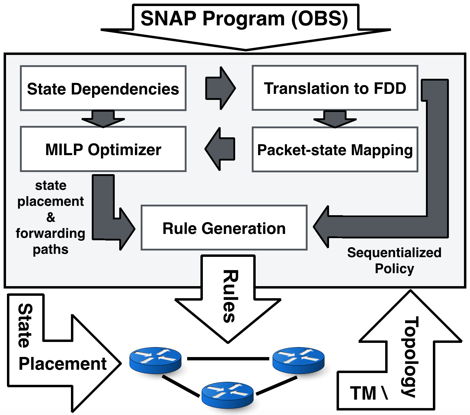
Figure 5: Overview of the compiler phases.

To implement a SNAP program specified on one big switch, we must fill in two critical details: traffic routing and state placement. The physical topology may offer many paths between edge ports, and many possible locations for placing state. The routing and placement problems interact: if two flows (with different input and output OBS ports) both need some state variable $s$, we should select routes for the two flows such that they pass through a common location where we place $s$. Further complicating the situation, the OBS program may specify that certain flows read/write multiple state variables in a particular order. The routing and placement on the physical topology must respect that order. In DNS-tunnel-detect, for instance, routing must ensure that packets reach wherever orphan is placed before susp-client. In some cases, two different flows may depend on the same state variables, but in different orders.

We have designed a compiler that translates OBS programs into forwarding rules and state placements for a given topology. As shown in Figure 5, the two key phases are (i) translation to extended forwarding decision diagrams (xFDDs)—used as the intermediate representation of the program and to calculate which flows need which state variables—and (ii) optimization via mixed integer linear program (MILP)—used to decide routing and state placement. In the rest of this section, we present the compilation process in phases, first discussing the analysis of state dependencies, followed by the translation to xFDDs and the packet-state mapping, then the optimization problems, and finally the generation of rules sent to the switches.

4.1 State Dependency Analysis

Given a program, the compiler first performs state dependency analysis to determine the ordering constraints on its state variables. A state variable $t$ depends on a state variable $s$ if the program writes to $t$ after reading from $s$. Any realization of the program on a concrete network must ensure that $t$ does not come before $s$. Parallel composition, $p+q$, introduces no dependencies: if $p$ reads or writes state, then $q$ can run independently of that. Sequential composition $p;q$, on the other hand, introduces dependencies: whatever reads are in $p$ must happen before writes in $q$. In explicit conditionals “$\text{if }a\text{ then }p\text{ else }q$”, the writes in $p$ and $q$ depend on the condition $a$. Finally, atomic sections $\mathsf{atomic}(p)$ say that all state in $p$ is inter-dependent. In DNS-tunnel-detect, for instance, blacklist is dependent on susp-client, itself dependent on orphan. This information is encoded as a dependency graph on state variables and is used to order the xFDD structure (§4.2), and in the MILP (§4.4) to drive state placement.

4.2 Extended Forwarding Decision Diagrams

$$\begin{array}[]{rclr}d&::=&t~{}?~{}d_{1}:d_{2}\,|\,\{as_{1},\dots,as_{n}\}&\text{xFDDs}\\ t&::=&f=v\,|\,f_{1}=f_{2}\,|\,s[e_{1}]=e_{2}&\text{tests}\\ as&::=&a\,|\,a;a&\text{action sequences}\\ a&::=&id\,|\,drop\,|\,f\leftarrow v\,|\,s[e_{1}]\leftarrow e_{2}&\text{actions}\\ &&\,|\,s[e_{1}]\text{\footnotesize{++}}\,|\,s[e_{1}]\text{\footnotesize{-{}-}}\\ \end{array}$$

$$\begin{array}[]{rcl}\textsc{to-xfdd}(a)&=&\{a\}\\ \textsc{to-xfdd}(f=v)&=&f=v~{}?~{}\{id\}~{}:~{}\{drop\}\\ \textsc{to-xfdd}(\neg x)&=&\ominus\textsc{to-xfdd}(x)\\ \textsc{to-xfdd}(s[e_{1}]=e_{2})&=&s[e_{1}]=e_{2}~{}?~{}\{id\}~{}:~{}\{drop\}\\ \textsc{to-xfdd}(\mathsf{atomic}(p))&=&\textsc{to-xfdd}(p)\\ \textsc{to-xfdd}(p+q)&=&\textsc{to-xfdd}(p)\oplus\textsc{to-xfdd}(q)\\ \textsc{to-xfdd}(p;q)&=&\textsc{to-xfdd}(p)\odot\textsc{to-xfdd}(q)\\ \textsc{to-xfdd}(\text{if }x\text{ then }p\text{ else }q)&=&(\textsc{to-xfdd}(x)\odot\textsc{to-xfdd}(p))\\ &\oplus{}&(\ominus\textsc{to-xfdd}(x)\odot\textsc{to-xfdd}(q))\end{array}$$

Figure 6: xFDD syntax and translation.

$\begin{array}[]{rcl}\{as_{11},\cdots,as_{1n}\}\oplus\{as_{21},\cdots,as_{2m}\}&=&\{as_{11},\cdots,as_{1n}\}\cup\{as_{21},\cdots,as_{2m}\}\\ (t~{}?~{}d_{1}:d_{2})\oplus\{as_{1},\cdots,as_{n}\}&=&(t~{}?~{}d_{1}\oplus\{as_{1},\cdots,as_{n}\}:d_{2}\oplus\{as_{1},\cdots,as_{n}\})\\ \\ (t_{1}~{}?~{}d_{11}:d_{12})\oplus(t_{2}~{}?~{}d_{21}:d_{22})&=&\begin{cases}(t_{1}~{}?~{}d_{11}\oplus d_{21}:d_{12}\oplus d_{22})&t_{1}=t_{2}\\ (t_{1}~{}?~{}d_{11}\oplus(t_{2}~{}?~{}d_{21}:d_{22}):d_{12}\oplus(t_{2}~{}?~{}d_{21}:d_{22})&t_{1}\sqsubset t_{2}\\ (t_{2}~{}?~{}d_{21}\oplus(t_{1}~{}?~{}d_{11}:d_{12}):d_{22}\oplus(t_{1}~{}?~{}d_{11}:d_{12})&t_{2}\sqsubset t_{1}\end{cases}\end{array}$

$\begin{array}[]{rcl}\ominus\{id\}&=&\{drop\}\\ \ominus\{drop\}&=&\{id\}\\ \ominus(t?d_{1}:d_{2})&=&(t?\ominus d_{1}:\ominus d_{2})\end{array}$

$\begin{array}[]{lcl}as\odot\{as_{1},\cdots,as_{n}\}&=&\{as\odot as_{1},\cdots,as\odot as_{n}\}\\ as\odot(t~{}?~{}d_{1}:d_{2})&=&\text{(see explanations in \textsection\ref{sec:fdds})}\\ \{as_{1},\cdots,as_{n}\}\odot d&=&(as_{1}\odot d)\oplus\cdots\oplus(as_{n}\odot d)\\ (t~{}?~{}d_{1}:d_{2})\odot d&=&(d_{1}\odot d)|_{t}\oplus(d_{2}\odot d)|_{\sim t}\\ \end{array}$

$\begin{array}[]{rcl}\{as_{1},\cdots,as_{n}\}|_{t}&=&(t~{}?~{}\{as_{1},\cdots,as_{n}\}:\{drop\})\\ \\ (t_{1}~{}?~{}d_{1}:d_{2})|_{t_{2}}&=&\begin{cases}(t_{1}~{}?~{}d_{1}:\{drop\})&t_{1}=t_{2}\\ (t_{2}~{}?~{}(t_{1}~{}?~{}d_{1}:d_{2}):\{drop\})&t_{2}\sqsubset t_{1}\\ (t_{1}~{}?~{}d_{1}|_{t_{2}}:d_{2}|_{t_{2}})&t_{1}\sqsubset t_{2}\end{cases}\end{array}$

Figure 7: Definitions of xFDD composition operators.

$\begin{array}[]{rcl}\oplus(\{as_{11},\cdots,as_{1n}\},\{as_{21},\cdots,as_{2m}\},context)&=&\{as_{11},\cdots,as_{1n}\}\cup\{as_{21},\cdots,as_{2m}\}\\ \oplus((t~{}?~{}d_{1}:d_{2}),\{as_{1},\cdots,as_{n}\},context)&=&\text{{let }}c_{T}=context.add(t)\text{{ in }}\\ &&\text{{let }}brch_{T}=\oplus(d_{1},\{as_{1},\cdots,as_{n}\},c_{T})\text{{ in }}\\ &&\text{{let }}c_{F}=context.add(\neg t)\text{{ in }}\\ &&\text{{let }}brch_{F}=\oplus(d_{2},\{as_{1},\cdots,as_{n}\},c_{T})\text{{ in }}\\ &&(t~{}?~{}brch_{T}:brch_{F})\\ \\ \oplus(d_{1},d_{2},context)&=&\text{{let }}(t_{1}~{}?~{}d_{11}:d_{12})=\textsc{refine}(d_{1},context)\text{{ in }}\\ &&\text{{let }}(t_{2}~{}?~{}d_{21}:d_{22})=\textsc{refine}(d_{2},context)\text{{ in }}\\ &&\text{{let }}c_{T}=\text{{ if }}t_{1}\sqsubset t_{2}\text{{ then }}context.add(t_{1})\text{{ else }}context.add(t_{2})\text{{ in }}\\ &&\text{{let }}c_{F}=\text{{ if }}t_{1}\sqsubset t_{2}\text{{ then }}context.add(\neg t_{1})\text{{ else }}context.add(\neg t_{2})\text{{ in }}\\ &&\begin{cases}(t_{1}~{}?~{}\oplus(d_{11},d_{21},c_{T}):\oplus(d_{12},d_{22},c_{F}))&t_{1}=t_{2}\\ (t_{1}~{}?~{}\oplus(d_{11},(t_{2}~{}?~{}d_{21}:d_{22}),c_{T}):\oplus(d_{12},(t_{2}~{}?~{}d_{21}:d_{22}),c_{F})&t_{1}\sqsubset t_{2}\\ (t_{2}~{}?~{}\oplus(d_{21},(t_{1}~{}?~{}d_{11}:d_{12}),c_{T}):\oplus(d_{22},(t_{1}~{}?~{}d_{11}:d_{12}),c_{F})&t_{2}\sqsubset t_{1}\end{cases}\end{array}$

$$\begin{array}[]{rcl}\textsc{refine}(\{as_{1},\cdots,as_{n}\},context)&=&\{as_{1},\cdots,as_{n}\}\\ \textsc{refine}((t~{}?~{}d_{1}:d_{2}),context)&=&\text{{if }}context.imply(t)\text{{ then }}\textsc{refine}(d_{1},context)\\ &&\text{{else if }}context.imply(\neg t)\text{{ then }}\textsc{refine}(d_{2},context)\\ &&\text{{else }}(t~{}?~{}d_{1}:d_{2})\\ \end{array}$$

Figure 8: A closer look at $\oplus$.

The input to the compiler is a SNAP program, which can be a composition of several smaller programs. The output, on the other end, is the distribution of the original policy across the network. Thus, in between, we need an intermediate representation for SNAP programs that is both composable and easily partitioned. This intermediate representation can help the compiler compose small program pieces into a unified representation, which can further be partitioned to get distributed across the network. Extended forwarding decision diagrams (xFDDs), which are introduced in this section, are what we use as our internal representation of SNAP programs and have both desired properties. They also simplify analysis of SNAP programs for extracting packet-state mapping, which we discuss in §4.3

Formally (see Figure 6), an xFDD is either a branch $(t~{}?~{}d_{1}:d_{2})$, where $t$ is a test and $d_{1}$ and $d_{2}$ are xFDDs, or a set of action sequences $\{as_{1},\dots,as_{n}\}$. Each branch can be thought of as a conditional: if the test $t$ holds on a given packet $pkt$, then the xFDD continues processing $pkt$ using $d_{1}$; if not, processes $pkt$ using $d_{2}$. There are three kinds of tests. The field-value test $f=v$ holds when $pkt.f$ is equal to $v$. The field-field test $f_{1}=f_{2}$ holds when the values in $pkt.f_{1}$ and $pkt.f_{2}$ are equal. Finally, the state test $s[e_{1}]=e_{2}$ holds when the state variable $s$ at index $e_{1}$ is equal to $e_{2}$. The last two tests are our extensions to FDDs. The state tests support our stateful primitives, and as we show later in this section, the field-field tests are required for correct compilation. Each leaf in an xFDD is a set of action sequences, with each action being either the identity, drop, field-update $f\leftarrow v$, or state update $s[e_{1}]\leftarrow e_{2}$, which is another extension to the original FDD.

A key property of xFDDs is that the order of their tests ($\sqsubset$) must be defined in advance. This ordering is necessary to ensure that each test is present at most once on any path in the final tree when merging two xFDDs into one. Thus, xFDD composition can be done efficiently without creating redundant tests. In our xFDDs, we ensure that all field-value tests precede all field-field tests, themselves preceding all state tests. Field-value tests themselves are ordered by fixing an arbitrary order on fields and values. Field-field tests are ordered similarly. For state tests, we first define a total order on state variables by looking at the dependency graph from §4.1. We break the dependency graph into strongly connected components (SCCs) and fix an arbitrary order on state variables within each SCC. For every edge from one SCC to another, i.e., where some state variable in the second SCC depends on some state variable in the first, $s_{1}$ precedes $s_{2}$ in the order, where $s_{2}$ is the minimal element in the second SCC and $s_{1}$ is the maximal element in the first SCC. The state tests are then ordered based on the order of state variables.

We translate a program to an xFDD using the to-xfdd function (Figure 6), which translates small parts of a program directly to xFDDs. Composite programs get recursively translated and then composed using a corresponding composition operator for xFDDs: we use $\oplus$ for $p+q$, $\odot$ for $p$ ; $q$, and $\ominus$ for $\neg p$. Figure 7 gives a high-level definition of the semantics of these operators. For example, $d_{1}\oplus d_{2}$ tries to merge similar test nodes recursively by merging their true branches together and false ones together. If the two tests are not the same and $d_{1}$’s test comes first in the total order, both of its subtrees are merged recursively with $d_{2}$. The other case is similar. $d_{1}\oplus d_{2}$ for leaf nodes is the union of their action sets.

The hardest case is surely for $\odot$, where we try to add in an action sequence $as$ to an xFDD $(t~{}?~{}d_{1}:d_{2})$. Suppose we want to compose $f\leftarrow v_{1}$ with $(f=v_{2}~{}?~{}d_{1}:d_{2})$. The result of this xFDD composition should behave as if we first do the update and then the condition on $f$. If $v_{1}=v_{2}$, the composition should continue only on $d_{1}$, and if not, only on $d_{2}$. Now let’s look at a similar example including state, composing $s[srcip]\leftarrow e_{1}$ with $(s[dstip]=e_{2}~{}?~{}d_{1}:d_{2})$. If $srcip$ and $dstip$ are equal (rare but not impossible) and $e_{1}$ and $e_{2}$ always evaluate to the same value, then the whole composition reduces to just $d_{1}$. The field-field tests are introduced to let us answer these equality questions, and that is why they always precede state tests in the tree. The trickiness in the algorithm comes from generating proper field-field tests, by keeping track of the information in the xFDD, to properly answer the equality tests of interest. The full algorithm is given in appendix B.

Note that the actual definition of the xFDD composition operators is a bit more involved than the one in Figure 7 as we have to make sure, while composing FDDs, that the resulting FDD is well-formed. An FDD is defined to be well-formed if its tests conform to the pre-defined total order ($\sqsubset$) and do not contradict the previous tests in the FDD. Figure 8 contains a more detailed definition of $\oplus$ as an example. To detect possible contradictions, we accumulate both the equalities and inequalities implied by previous tests in an argument called $context$ and pass it through recursive calls to $\oplus$. Before applying $\oplus$ to the input FDDs, we first run each of the FDDs through a function called refine, which removes both redundant and contradicting tests from top of the input FDD based on the input $context$ until it reaches a non-redundant and non-contradicting test. After both input FDDs are “refined”, we continue with the merge as before.

Finally, recall from §3 that Inconsistent use of state variables is prohibited by the language semantics when composing programs. We enforce the semantics by looking for these violations while merging the xFDDs of composed programs and raising a compile error if the final xFDD contains a leaf with parallel updates to the same state variable.

4.3 Packet-State Mapping

For a given program $p$, the corresponding xFDD $d$ offers an explicit and complete specification of the way $p$ handles packets. We analyze $d$, using an algorithm called packet-state mapping, to determine which flows use which states. This information is further used in the optimization problem (§4.4) to decide the correct routing for each flow. Our default definition of a flow is those packets that travel between any given pair of ingress/egress ports in the OBS, though we can use other notions of flow (see §4.4). Traversing from $d$’s root down to the action sets at $d$’s leaves, we can gather information associating each flow with the set of state variables read or written. See appendix E for the full algorithm.

Furthermore, the operators can give hints to the compiler by specifying their network assumptions in a separate policy:

assumption = (srcip = 10.0.1.0/24 & inport = 1)
                   + (srcip = 10.0.2.0/24 & inport = 2)
                   + ...
                   + (srcip = 10.0.6.0/24 & inport = 6)

We require the assumption policy to be a predicate over packet header fields, only passing the packets that match the operator’s assumptions. assumption is then sequentially composed with the rest of the program, enforcing the assumption by dropping packets that do not match the assumption. Such assumptions benefit the packet-state mapping. Consider our example xFDD in Figure 3. Following the xFDD’s tree structure, we can infer that all the packets going to port 6 need all the three state variables in DNS-tunnel-detect. We can also infer that all the packets coming from the 10.0.6.0/24 subnet need orphan and susp-client. However, there is nothing in the program to tell the compiler that these packets can only enter the network from port 6. Thus, the above assumption policy can help the compiler to identify this relation and place state more efficiently.

4.4 State Placement and Routing

At this stage, the compiler has enough information to fill in the details abstracted away from the programmer: where and how each state variable should be placed, and how the traffic should be routed in the network. There are two general approaches for deciding state placement and routing. One is to keep each state variable at one location and route the traffic through the state variables it needs. The other is to keep multiple copies of the same state variable on different switches and partition and route the traffic through them. The second approach requires mechanisms to keep different copies of the same state variable consistent. However, it is not possible to provide strong consistency guarantees when distributed updates are made on a packet-by-packet basis at line rate. Therefore, we chose the first approach, which locates each state variable at one physical switch.

To decide state placement and routing, we generate an optimization problem, a mixed-integer linear program (MILP) that is an extension of the multi-commodity flow linear program. The MILP has three key inputs: the concrete network topology, the state dependency graph $G$, and the packet-state mapping, and two key outputs: routing and state placement (Table 1). Since route selection depends on state placement and each state variable is constrained to one physical location, we need to make sure the MILP picks correct paths without degrading network performance. Thus, the MILP minimizes the sum of link utilization in the network as a measure of congestion. However, other objectives or constraints are conceivable to customize the MILP to other kinds of performance requirements.

Inputs. The topology is defined in terms of the following inputs to the MILP: 1 the nodes, some distinguished as edges (ports in OBS), 2 expected traffic $d_{uv}$ for every pair of edge nodes $u$ and $v$, and 3 link capacities $c_{ij}$ for every pair of nodes $i$ and $j$. State dependencies in $G$ are translated into input sets $dep$ and $tied$. $tied$ contains pairs of state variables which are in the same SCC in $G$, and must be co-located. $dep$ identifies state variables with dependencies that do not need to be co-located; in particular, $(s,t)\in dep$ when $s$ precedes $t$ in variable ordering, and they are not in the same SCC in $G$. The packet-state mapping is used as the input variables $S_{uv}$, identifying the set of state variables needed on flows between nodes $u$ and $v$.

Variable	Description
$u,v$	edge nodes (ports in OBS)
$n$	physical switches in the network
$i,j$	all nodes in the network
$d_{uv}$	traffic demand between $u$ and $v$
$c_{ij}$	link capacity between $i$ and $j$
$dep$	state dependencies
$tied$	co-location dependencies
$S_{uv}$	state variables needed for flow $uv$
$R_{uvij}$	fraction of $d_{uv}$ on link $(i,j)$
$P_{sn}$	1 if state $s$ is placed on $n$, 0 otherwise
$P_{suvij}$	$d_{uv}$ fraction on link ($i,j$) that has passed $s$

Table 1: Inputs and outputs of the optimization problem.

Outputs and Constraints. The routing outputs are variables $R_{uvij}$, indicating what fraction of the flow from edge node $u$ to $v$ should traverse the link between nodes $i$ and $j$. The constraints on $R_{uvij}$ (left side of Table 2) follow the multi-commodity flow problem closely, with standard link capacity and flow conservation constraints, and edge nodes distinguished as sources and sinks of traffic.

State placement is determined by the variables $P_{sn}$, which indicate whether the state variable $s$ should be placed on the physical switch $n$. Our constraints here are more unique to our setting. First, every state variable $s$ can be placed on exactly one switch, a choice we discussed earlier in this section. Second, we must ensure that flows that need a given state variable $s$ traverse that switch. Third, we must ensure that each flow traverses states in the order specified by the $dep$ relation; this is what the variables $P_{suvij}$ are for. We require that $P_{suvij}=R_{uvij}$ when the traffic from $u$ to $v$ that goes over the link $(i,j)$ has already passed the switch with the state variable $s$, and zero otherwise. If $dep$ requires that $s$ should come before some other state variable $t$—and if the $(u,v)$ flow needs both $s$ and $t$—we can use $P_{suvij}$ to make sure that the $(u,v)$ flow traverses the switch with $t$ only after it has traversed the switch with $s$ (the last state constraint in Table 2). Finally, we must make sure that state variables $(s,t)\in tied$ are located on the same switch. Note that only state variables that are inter-dependent are required to be located on the same switch. Two variables $s$ and $t$ are inter-dependent if a read from $s$ is required before a write to $t$ and vice versa. Placing them on different switches will result in a forwarding loop between the two switches which is not desirable in most networks. Therefore, in order to synchronize reads and writes to inter-dependent variables correctly, they are always placed on the same switch.

Although the current prototype chooses the same path for the traffic between the same ports, the MILP can be configured to decide paths for more fine-grained notions of flows. Suppose packet-state mapping finds that only packets with $srcip=x$ need state variable $s$. We refine the MILP input to have two edge nodes per port, one for traffic with $srcip=x$ and one for the rest, so the MILP can choose different paths for them.

Finally, the MILP makes a joint decision for state placement and routing. Therefore, path selection is tied to state placement. To have more freedom in picking forwarding paths, one option is to first use common traffic engineering techniques to decide routing, and then optimize the placement of state variables with respect to the selected paths. However, this approach may require replicating state variables and maintaining consistency across multiple copies, which as mentioned earlier, is not possible at line rate for distributed packet-by-packet updates to state variables.

4.5 Generating Data-Plane Rules

Rule generation happens in two phases and combines information from the xFDD and MILP to configure the network switches. We assume each packet is augmented with a SNAP-header upon entering the network, which contains its original OBS inport and future outport, and the id of the last processed xFDD node, the purpose of which will be explained shortly. This header is stripped off by the egress switch when the packet exits the network. We use DNS-tunnel-detect;assign-egress from §2 as a running example, with its xFDD in Figure 3. For the sake of the example, we assume that all the state variables are stored on $C_{6}$ instead of $D_{4}$.

Routing Constraints	State Constraints
	$\sum_{n}P_{sn}=1$
$\sum_{j}R_{uvuj}=1$	$\forall u,v.~{}\forall s\in S_{uv}.~{}\sum_{i}R_{uvin}\geq P_{sn}$
$\sum_{i}R_{uviv}=1$	$\forall(s,t)\in tied.~{}P_{sn}=P_{tn}$
$\sum_{u,v}R_{uvij}d_{uv}\leq c_{ij}$	$P_{suvij}\leq R_{uvij}$
$\sum_{i}R_{uvin}=\sum_{j}R_{uvnj}$	$P_{sn}+\Sigma_{i}P_{suvin}=\Sigma_{j}P_{suvnj}$
$\sum_{i}R_{uvin}\leq 1$	$\forall s\in S_{uv}.~{}P_{sv}+\sum_{i}P_{suviv}=1$
	$P_{sn}+\Sigma_{i}P_{suvin}\geq P_{tn}$

Table 2: Constraints of the optimization problem.

In the first phase, we break the xFDD down into ‘per-switch’ xFDDs, since not every switch needs the entire xFDD to process packets. Splitting the xFDD is straightforward given placement information: stateless tests and actions can happen anywhere, but reads and writes of state variables must happen on switches storing them. For example, edge switches ($I_{1}$ and $I_{2}$, and $D_{1}$ to $D_{4}$) only need to process packets up to the state tests, e.g., tests 3 and 8, and write the test number in the packet’s SNAP-header showing how far into the xFDD they progressed. Then, they send the packets to $C_{6}$, which has the corresponding state variables, orphan and susp-client. $C_{6}$, on the other hand, does not need the top part of the xFDD. It just needs the subtrees containing its state variables to continue processing the packets sent from the edges. The per-switch xFDDs are then translated to switch-level configurations, by a straightforward traversal of the xFDD (See §5).

In the second phase, we generate a set of match-action rules that take packets through the paths decided by the MILP. These paths comply with the state ordering used in the xFDD, thus they get packets to switches with the right states in the right order. Note that packets contain the path identifier (the OBS inport and outport, $(u,v)$ pair in this case) and the “routing” match-action rules are generated in terms of this identifier to forward them on the correct path. Additionally, note that it may not always be possible to decide the egress port $v$ for a packet upon entry if its outport depends on state. We observe that in that case, all the paths for possible outports of the packet pass the state variables it needs. We load-balance over these paths in proportion to their capacity and show, in appendix D, that traffic on these paths remains in their capacity limit.

To see an example of how packets are handled by generated rules, consider a DNS response with source IP 10.0.1.1 and destination IP 10.0.6.6, entering the network from port 1. The rules on $I_{1}$ process the packet up to test 8 in the xFDD, tag the packet with the path identifier (1, 6) and number 8. The packet is then sent to $C_{6}$. There, $C_{6}$ will process the packet from test 8, update state variables accordingly, and send the packet to $D_{4}$ to exit the network from port 6.

5 Implementation

The compiler is mostly implemented in Python, except for the state placement and routing phase (§4.4) which uses the Gurobi Optimizer [15] to solve the MILP. The compiler’s output for each switch is a set of switch-level instructions in a low-level language called NetASM [32], which comes with a software switch capable of executing those instructions. NetASM is an assembly language for programmable data planes designed to serve as the “narrow waist” between high-level languages such as SNAP, and NetCore[19], and programmable switching architectures such as RMT [7], FPGAs, network processors and Open vSwitch.

As described in §4.5, each switch processes the packet by its customized per-switch xFDD, and then forwards it based on the fields of the SNAP-header using a match-action table. To translate the switch’s xFDD to NetASM instructions, we traverse the xFDD and generate a branch instruction for each test node, which jumps to the instruction of either the true or false branch based on the test’s result. Moreover, we generate instructions to create two tables for each state variable, one for the indices and one for the values. In the case of a state test in the xFDD, we first retrieve the value corresponding to the index that matches the packet, and then perform the branch. For xFDD leaf nodes, we generate store instructions that modify the packet fields and state tables accordingly. Finally, we use NetASM support for atomic execution of multiple instructions to guarantee that operations on state tables happen atomically.

While NetASM was useful for testing our compiler, any programmable device that supports match-action tables, branch instructions, and stateful operations can be a SNAP target. The prioritized rules in match-action tables, for instance, are effectively branch instructions. Thus, one can use multiple match-action tables to implement xFDD in the data plane, generating a separate rule for each path in the xFDD. Several emerging switch interfaces support stateful operations [6, 4, 38, 25]. We discuss possible software and hardware implementations for SNAP stateful operations in §7.

6 Evaluation

This section evaluates SNAP in terms of language expressiveness and compiler performance.

6.1 Language Expressiveness

	Application
Chimera [5]	# domains sharing the same IP address
	# distinct IP addresses under the same domain
	DNS TTL change tracking
	DNS tunnel detection
	Sidejack detection
	Phishing/spam detection
FAST [21]	Stateful firewall
	FTP monitoring
	Heavy-hitter detection
	Super-spreader detection
	Sampling based on flow size
	Selective packet dropping (MPEG frames)
	Connection affinity
Bohatei [8]	SYN flood detection
	DNS amplification mitigation
	UDP flood mitigation
	Elephant flows detection
Others	Bump-on-the-wire TCP state machine
	Snort flowbits [36]

Table 3: Applications written in SNAP.

We have implemented several stateful network functions (Table 3) that are typically relegated to middleboxes in SNAP. Examples were taken from the Chimera [5], FAST [21], and Bohatei [8] systems. The code can be found in appendix F. Most examples use protocol-related fields in fixed packet-offset locations, which are parsable by emerging programmable parsers. Some fields require session reassembly. However, this is orthogonal to the language expressiveness; as long as these fields are available to the switch, they can be used in SNAP programs. To make them available, one could extract these fields by placing a “preprocessor” before the switch pipeline, similar to middleboxes. For instance, Snort [36] uses preprocessors to extract fields for use in the detection engine.

6.2 Compiler Performance

The compiler goes through several phases upon the system’s cold start, yet most events require only some of them. Table 4 summarizes these phases and their sensitivity to network and policy changes.

Cold Start. When the very first program is compiled, the compiler goes through all phases, including MILP model creation, which happens only once in the lifetime of the network. Once created, the model supports incremental additions and modifications of variables and constraints in a few milliseconds.

Policy Changes. Compiling a new program requires executing the three program analysis phases and rule generation as well as both state placement and routing, which are decided using the MILP in §4.4, denoted by “ST”. Policy changes become considerably less frequent (§2.2) since most dynamic changes are captured by the state variables that reside on the data plane. The policy, and consequently switch configurations, do not change upon state changes. Thus, we expect policy changes to happen infrequently, and be planned in advance. The Snort rule set, for instance, gets updated every few days [37].

Topology/TM Changes. Once the policy is compiled, we fix the decided state placement, and only re-optimize routing in response to network events such as failures. For that, we formulated a variant of ST, denoted as “TE” (traffic engineering), that receives state placement as input, and decides forwarding paths while satisfying state requirement constraints. We expect TE to run every few minutes since in a typical network, the traffic matrix is fairly stable and traffic engineering happens on the timescale of minutes [16, 42, 22, 41].

ID	Phase		Topo/TM Change	Policy Change	Cold Start
P1	State dependency		-	✓	✓
P2	xFDD generation		-	✓	✓
P3	Packet-state map		-	✓	✓
P4	MILP creation		-	-	✓
P5	MILP solving	State placement and routing (ST)	-	✓	✓
		Routing (TE)	✓	-	-
P6	Rule generation		✓	✓	✓

Table 4: Compiler phases. For each scenario, phases that get executed are checkmarked.

6.2.1 Experiments

We evaluated performance based on applications listed in Table 3. Traffic matrices are synthesized using a gravity model [31]. We used an Intel Xeon E3, 3.4 GHz, 32GB server, and PyPy compiler [27].

Topology	# Switches	# Edges	# Demands
Stanford	26	92	20736
Berkeley	25	96	34225
Purdue	98	232	24336
AS 1755	87	322	3600
AS 1221	104	302	5184
AS 6461	138	744	9216
AS 3257	161	656	12544

Table 5: Statistics of evaluated enterprise/ISP topologies.

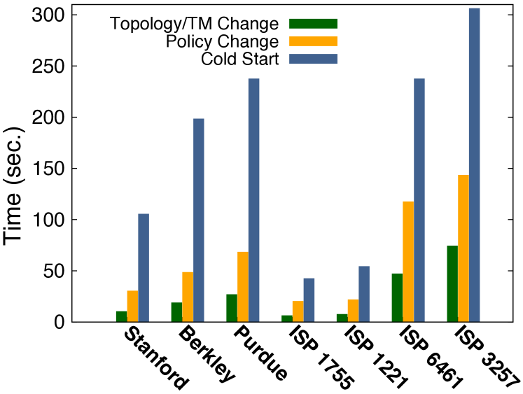
Figure 9: Compilation time of DNS-tunnel-detect with routing on enterprise/ISP networks.

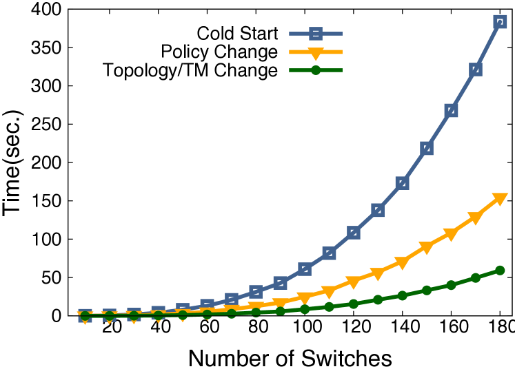
Figure 10: Compilation time of DNS-tunnel-detect with routing on IGen topologies.

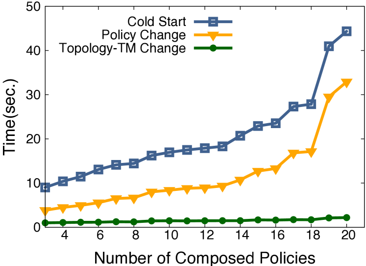
Figure 11: Compilation time for policies from Table 3 incrementally composed on a 50-switch network.

Figure 12: Compiler runtimes for scenarios in Table 4 on various policies and topologies. Once compiled for the first time (cold start, policy change), a policy reacts to traffic using its state variables. Topology/TM changes result in reoptimizing forwarding paths.

	P1-P2-P3 (s)	P5 (s)		P6(s)	P4 (s)
		ST	TE
Stanford	1.1	29	10	0.1	75
Berkeley	1.5	47	18	0.1	150
Purdue	1.2	67	27	0.1	169
AS 1755	0.6	19	6	0.04	22
AS 1221	0.7	21	7	0.04	32
AS 6461	0.8	116	47	0.1	120
AS 3257	0.9	142	74	0.2	163

Table 6: Runtime of compiler phases when compiling DNS-tunnel-detect with routing on enterprise/ISP topologies.

Topologies. We used a set of three campus networks and four inferred ISP topologies from RocketFuel [40] (Table 5). For ISP networks, we considered 70% of the switches with the lowest degrees as edge switches to form OBS external ports. The “# Demands” column shows the number of distinct OBS ingress/egress pairs. We assume directed links. Table 6 shows compilation time for the DNS tunneling example (§2) on each network, broken down by compiler phase. Figure 12 compares the compiler runtime for different scenarios, combining the runtimes of phases relevant for each.

Scaling with topology size. We synthesize networks with 10–180 switches using IGen [29]. In each network, 70% of the switches with the lowest degrees are chosen as edges and the DNS tunnel policy is compiled with that network as a target. Figure 12 shows the compilation time for different scenarios, combining the runtimes of phases relevant for each. Note that by increasing the topology size, the policy size also increases in the assign-egress and assumption parts.

Scaling with number of policies. The performance of several phases of the compiler, specially xFDD generation, is a function of the size and complexity of the input policy. Therefore, we evaluated how the compiler’s performance scales with policy size using the example programs from Table 3. Given that these programs are taken from recent papers and tools in the literature [5, 21, 8, 36], we believe they form a fair benchmark for our evaluation. Except for TCP state machine, the example programs are similar in size and complexity to the DNS tunnel example (§2). We use the 50-switch network from the previous experiment and start with the first program in Table 3. We then gradually increase the size of the final policy by combining this program with more programs from Table 3 using the parallel composition operator. Each additional component program affects traffic destined to a separate egress port.

Figure 12 depicts the compilation time as a function of the number of components from Table 3 that form the final policy. The $10$-second jump from 18 to 19 takes place when the TCP state machine policy is added, which is considerably more complex than others. The increase in the compilation time mostly comes from the xFDD generation phase. In this phase, the composed programs are transformed into separate xFDDs, which are then combined to form the xFDD for the whole policy (§4.2). The cost of xFDD composition depends on the size of the operands, so as more components are put together, the cost grows. The cost may also depend on the order of xFDD composition. Our current prototype composes xFDDs in the same order as the programs themselves are composed and leaves finding the optimal order to compose xFDDs to future work.

The last data point in Figure 12 shows the compilation time of a policy composed of all the 20 examples in Table 3, with a total of 35 state variables. These policies are composed using parallel composition, which does not introduce read/write dependencies between state variables. Thus, the dependency graph for the final policy is a collection of the dependency graphs of the composed policies. Each of the composed policies affects the traffic to a separate egress port, which is detected by the compiler in the packet-state mapping phase. Thus, when compiled to the 50-switch network, state variables for each policy are placed on the switch closest to the egress port whose traffic the policy affects. If a policy were to affect a larger portion of traffic, e.g., the traffic of a set of ingress/egress ports, SNAP would place state variables in an optimal location where the aggregated traffic of interest is passing through.

6.2.2 Analysis of Experimental Results

Creating the MILP takes longer than solving it, in most cases, and much longer than other phases. Fortunately, this is a one-time cost. After creating the MILP instance, incrementally adding or removing variables and constraints (as the topology and/or state requirements change) takes just a few milliseconds.

Solving the ST MILP unsurprisingly takes longer as compared to the rest of the phases when topology grows. It takes $\scriptsize\sim$ 2.5 minutes for the biggest synthesized topology and $\scriptsize\sim$ 2.3 minutes for the biggest RocketFuel topology. The curve is close to exponential as the problem is inherently computationally hard. However, this phase takes place only in cold start or upon a policy change, which are infrequent and planned in advance.

Re-optimizing routing with fixed state placement is much faster. In response to network events (e.g., link failures), TE MILP can recompute paths in around a minute across all our experiments, which is the timescale we initially expected for this phase as it runs in the topology/TM change scenarios. Moreover, it can be used even on policy changes, if the user settles for a sub-optimal state placement using heuristics rather than ST MILP. We plan to explore such heuristics.

Given the kinds of events that require complete (policy change) or partial (network events) recompilation, we believe that our compilation techniques meet the requirements of enterprise networks and medium-size ISPs. Moreover, if needed, our compilation procedure could be combined with traffic-engineering techniques once the state placement is decided, to avoid re-solving the original or even TE MILP on small timescales.

7 Discussion

This section discusses data-plane implementation strategies for SNAP’s stateful operations, how SNAP relates to middleboxes, and possible extensions to our techniques to enable a broader range of applications.

7.1 Stateful Operations in the Data Plane

A state variable (array) in SNAP is a key-value mapping, or a dictionary, on header fields, persistent across multiple packets. When the key (index) range is small, it is feasible to pre-allocate all the memory the dictionary needs and implement it using an array. A large but sparse dictionary can be implemented using a reactively-populated table, similar to a MAC learner table. It contains a single default entry in the beginning, and as packets fly by and change the state variable, it reactively adds/updates the corresponding entries.

In software, there are efficient techniques to implement a dictionary in either approach, and some software switches already support similar reactive “learning” operations, either atomically [32] or with small periods of inconsistency [25]. The options for current hardware are: 1 arrays of registers, which are already supported in emerging switch interfaces [6]. They can be used to implement small dictionaries, as well as Bloom Filters and hash tables as sparse dictionaries. In the latter case, it is possible for two different keys to hash to the same dictionary entry. However, there are applications such as load balancing and flow-size-based sampling that can tolerate such collisions [21]. 2 Content Addressable Memories (CAMs) are typically present in today’s hardware switches and can be modified by a software agent running on the switch. Since CAM updates triggered by a packet are not immediately available to the following packets, it may be used for applications that tolerate small periods of state inconsistency, such as a MAC learner, DNS tunnel detection, and others from Table 3. Our NetASM implementation (§5) takes the CAM-based approach. NetASM’s software switch supports atomic updates to the tables in the data plane and therefore can perform consistent stateful operations.

At the time of writing this paper, we are not aware of any hardware switch that can implement an arbitrary number of SNAP’s stateful operations both at line rate and with strong consistency. Therefore, we use NetASM’s low-level primitives as the compiler’s backend so that we can specify data-plane primitives that are required for an efficient and consistent implementation of SNAP’s operations. If one is willing to relax one of the above constraints for a specific application, i.e., operating at line rate or strong consistency, it would be possible to implement SNAP on today’s switches. If strong consistency is relaxed, CAMs/TCAMs can be programmed using languages such as P4 [6] to implement SNAP’s stateful operations as described above. If line-rate processing is relaxed, one can use software switches, or programmable hardware switching devices such as ones in the OpenNFP project that allow insertion of Micro-C code extensions to P4 programs at the expense of processing speed [23] or FPGAs.

7.2 SNAP and Middleboxes

Networks traditionally rely on middleboxes for advanced packet processing, including stateful functionalities. However, advances in switch technology enable stateful packet processing in the data plane, which naturally makes the switches capable of subsuming a subset of middlebox functionality. SNAP provides a high-level programming framework to exploit this ability, hence, it is able to express a wide range of stateful programs that are typically relegated to middleboxes (see Table 3 for examples). This helps the programmer to think about a single, explicit network policy, as opposed to a disaggregated, implicit network policy using middleboxes, and therefore, get more control and customization over a variety of simpler stateful functionalities.

This also makes SNAP subject to similar challenges as managing stateful middleboxes. For example, many network functions must observe all traffic pertaining to a connection in both directions. In SNAP, if traffic in both directions uses a shared state variable, the MILP optimizer forces traffic in both directions through the same node. Moreover, previous work such as Split/Merge [30] and OpenNF [13] show how to migrate internal state from one network function to another, and Gember-Jacobson et al. [12] manage to migrate state without buffering packets at the controller. SNAP currently focuses on static state placement. However, since SNAP’s state variables are explicitly declared as part of the policy, rather than hidden inside blackbox software, SNAP is well situated to adopt these algorithms to support smooth transitions of state variables in dynamic state placement. Additionally, the SNAP compiler can easily analyze a program to determine whether a switch modifies packet fields to ensure correct traffic steering—something that is challenging today with blackbox middleboxes [9, 28].

While SNAP goes a step beyond previous high-level languages to incorporate stateful programming into SDN, we neither claim that it is as expressive as all stateful middleboxes, nor that it can replace them. To interact with middleboxes, SNAP may adopt techniques such as FlowTags [9] or SIMPLE [28] to direct traffic through middleboxs chains by tagging packets to mark their progress. Since SNAP has its own tagging and steering to keep track of the progress of packets through the policy’s xFDD, this adoption may require integrating tags in the middlebox framework with SNAP’s tags. As an example, we will describe below how SNAP and FlowTags can be used together on the same network.

In FlowTags, users specify which class of traffic should pass which chain of middleboxes under what conditions. For instance, they can ask for web traffic to go to an intrusion detection system (IDS) after a firewall if the firewall marks the traffic as suspicious. The controller keeps a mapping between the tags and the flow’s original five tuple plus the contextual information of the last middlebox, e.g., suspicious vs. benign in the case of a firewall. The tags are used for steering the traffic through the right chain of middleboxes and preserving the original information of the flow in case it is changed by middleboxes. To use FlowTags with SNAP, we can treat middlebox contexts as state variables and transform FlowTags policies to SNAP programs. Thus, they can be easily composed with other SNAP policies. Next, we can fix the placement of middlebox state variables to the actual location of the middlebox in the network in SNAP’s MILP. This way, SNAP’s compiler can decide state placement and routing for SNAP’s own policies while making sure that the paths between different middleboxes in the FlowTags policies exist in the network. Thus, steering happens using SNAP-generated tags. Middleboxes can still use tags from FlowTags to learn about flow’s original information or the context of the previous middlebox.

Finally, we focus on programming networks but if verification is of interest in future work, one might adopt techniques such as RONO [24] to verify isolation properties in the presence of stateful middleboxes. In summary, interacting with existing middleboxes is no harder or easier in SNAP than it is in other global SDN languages, stateless or stateful, such as NetKAT [2] or Stateful NetKAT [18].

7.3 Extending SNAP

Sharding state variables. The MILP assigns each state variable to one physical switch to avoid the overhead of synchronizing multiple instances of the same variable. Still, distributing a state variable remains a valid option. For instance, the compiler can partition $s[inport]$ into $k$ disjoint state variables, each storing $s$ for one port. The MILP can decide placement and routing as before, this time with the option of distributing partitions of $s$ with no concerns for synchronization. See appendix C for more details.

Fault-Tolerance. SNAP’s current prototype does not implement any particular fault tolerance mechanism in case a switch holding a state variable fails. Therefore, the state on the failed switch will be lost. However, this problem is not inherent or unique to SNAP and will happen in existing solutions with middleboxes too if the state of the middlebox is not replicated. Applying common fault tolerance techniques to switches with state to avoid state loss in case of failure can be an interesting direction for future work.

Modifying fields with state variables. An interesting extension to SNAP is allowing a packet field to be directly modified with the value of a state variable at a specific index: f <- s[e]. This action can be used in applications such as NATs and proxies, which can store connection mappings in state variables and modify packets accordingly as they fly by. Moreover, this action would enable SNAP programs to modify a field by the output of an arbitrary function on a set of packet fields, such as a hash function. Such a function is nothing but a fixed mapping between input header fields and output values. Thus, when analyzing the program, the compiler can treat these functions as fixed state variables with the function’s input fields as index for the state variable and place them on switches with proper capabilities when distributing the program across the network. However, adding this action results in complicated dependencies between program statements, which is interesting to explore as future work.

Deep packet inspection (DPI). Several applications such as intrusion detection require searching the packet’s payload for specific patterns. SNAP can be extended with an extra field called content, containing the packet’s payload. Moreover, the semantics of tests on the content field can be extended to match on regular expressions. The compiler can also be modified to assign content tests to switches with DPI capabilities.

Resource constraints. SNAP’s compiler optimizes state placement and routing for link utilization. However, other resources such as switch memory and processing power in terms of maximum number of complicated operations on packets (such as stateful updates, increments, or decrements) may limit the possible computations on a switch. An interesting direction for future work would be to augment the SNAP compiler with the ability to optimize for these additional resources.

Cross-packet fields. Layer 4-7 fields are useful for classifying flows in stateful applications, but are often scattered across multiple physical packets. Middleboxes typically perform session reconstruction to extract these fields. Although SNAP language is agnostic to the chosen set of fields, the compiler currently supports fields stored in the packet itself and the state associated with them. However, it may be interesting to explore abstractions for expressing how multiple packets (e.g., in a session) can form “one big packet” and use its fields. The compiler can further place sub-programs that use cross-packet fields on devices that are capable of reconstructing the “one big packet”.

Queue-based policies. SNAP currently has no notion of queues and therefore, cannot be used to express queue-based performance-oriented policies such as active queue management, queue-based load balancing, and packet scheduling. There is ongoing research on finding the right set of primitives for expressing such policies [34], which is largely orthogonal and complementary to SNAP’s current goals.

8 Related Work

Stateful languages. Stateful NetKAT [18], developed concurrently with SNAP, is a stateful language for “event-driven” network programming, which guarantees consistent update when transitioning between configurations in response to events. SNAP source language is richer and exponentially more compact than stateful NetKAT as it contains multiple arrays (as opposed to one) that can be indexed and updated by contents of packet headers (as opposed to constant integers only). Moreover, they place multiple copies of state at the edge, proactively generate rules for all configurations, and optimize for rule space, while we distribute state and optimize for congestion. Kinetic [17] provides a per-flow state machine abstraction, and NetEgg [44] synthesizes stateful programs from user’s examples. However, they both keep the state at the controller.

Compositional languages. NetCore [19], and other similar languages [20, 10, 2], have primitives for tests and modifications on packet fields as well as composition operators to combine programs. SNAP builds on these languages by adding primitives for stateful programming (§3). To capture the joint intent of two policies, sometimes the programmer needs to decompose them into their constituent pieces, and then reassemble them using ; and +. PGA [26] allows programmers to specify access control and service chain policies using graphs as the basic building block, and tackles this challenge by defining a new type of composition. However, PGA does not have linguistic primitives for stateful programming, such as those that read and write the contents of global arrays. Thus, we view SNAP and PGA as complementary research projects, with each treating different aspects of the language design space.

Stateful switch-level mechanisms. FAST [21] and OpenState [4] propose flow-level state machines as a primitive for a single switch. SNAP offers a network-wide OBS programming model, with a compiler to distribute the programs across the network. Thus, although SNAP is exponentially more compact than a state machine in cases where state is indexed by contents of packet header fields, both FAST and OpenState can be used as a target for a subset of SNAP programs.

Optimizing placement and routing. Several projects have explored optimizing placement of middleboxes and/or routing traffic through them. These projects and SNAP share the mathematical problem of placement and routing on a graph. Merlin programs specify service chains as well as optimization objectives [39], and the compiler uses an MILP to choose paths for traffic with respect to specification. However, it does not decide the placement of service boxes itself. Rather, it chooses the paths to pass through the existing instances of the services in the physical network. Stratos [11] explores middlebox placement and distributing flows amongst them to minimize inter-rack traffic, and Slick [3] breaks middleboxes into fine-grained elements and distributes them across the network while minimizing congestion. However, they both have a separate algorithm for placement. In Stratos, placement results is used in an ILP to decide distribution of flows. Slick uses a virtual topology on the placed elements with heuristic link weights, and finds shortest paths between traffic endpoints.

9 Conclusion

In this paper, we introduced a stateful SDN programming model with a one-big-switch abstraction, persistent global arrays, and network transactions. We developed algorithms for analyzing and compiling programs, and distributing their state across the network. Based on these ideas, we prototyped and evaluated the SNAP language and compiler on numerous sample programs. We also explore several possible extensions to SNAP to support a wider range of stateful applications. Each of these extensions introduces new and interesting research problems to extend our language, compilation algorithms, and prototype.

Appendix A Formal Semantics of SNAP

$$\begin{array}[]{rcl}v\in\mathsf{Val}&::=&\textsf{IP addresses}\,|\,\textsf{TCP ports}\,|\,\dots\,|\,\overset{\rightharpoonup}{v}\\ l\in\mathsf{Log}&::=&\mathsf{E}\,|\,R\,s\cup l\,|\,W\,s\cup l\\ &&\\ E\cup l&=&l\\ (R\,s,l_{1})\cup l_{2}&=&l_{1}\cup(R\,s,l_{2})\\ (W\,s,l_{1})\cup l_{2}&=&l_{1}\cup(W\,s,l_{2})\end{array}$$ $\mathsf{eval}_{e}:\mathsf{Expr}\rightarrow\mathsf{Packet}\rightarrow\mathsf{Val}$ $$\begin{array}[]{rcl}\mathsf{eval}_{e}(v,pkt)&=&v\\ \mathsf{eval}_{e}(f,pkt)&=&pkt.f\\ \mathsf{eval}_{e}(\overset{\rightharpoonup}{e},pkt)&=&\mathsf{eval}_{e}(e_{1},pkt),\dots,\mathsf{eval}_{e}(e_{n},pkt)\\ \lx@intercol\hfil\text{where }\overset{\rightharpoonup}{e}=e_{1},\dots,e_{n}\lx@intercol\end{array}$$ $\mathsf{eval}:\mathsf{Pol}\rightarrow\mathsf{Store}\rightarrow\mathsf{Packet}\rightarrow\mathsf{\mathsf{Store}}\times 2^{\mathsf{Packet}}\times\mathsf{Log}$ $$\begin{array}[]{lll}\mathsf{eval}(0,m,pkt)&=&(m,\emptyset,\mathsf{E})\\ \mathsf{eval}(1,m,pkt)&=&(m,\{pkt\},\mathsf{E})\\ \mathsf{eval}(f=v,m,pkt)&=&(m,\begin{cases}\{pkt\}&pkt.f=v\\ \emptyset&\text{otherwise}\end{cases},\mathsf{E})\\ \mathsf{eval}(s[e_{1}]=e_{2},m,pkt)&=&(m,\begin{cases}\{pkt\}&m~{}s~{}\mathsf{eval}_{e}(e_{1},pkt)=\mathsf{eval}_{e}(e_{2},pkt)\\ \emptyset&\text{otherwise}\end{cases},R\,s)\\ \mathsf{eval}(\neg a,m,pkt)&=&\text{ let }(\_,PKT,l)=\mathsf{eval}(a,m,pkt)\text{ in }(m,\{pkt\}\setminus PKT,l)\\ \mathsf{eval}(f\leftarrow v,m,pkt)&=&(m,pkt[f\mapsto v],\mathsf{E})\\ \mathsf{eval}(s[e_{1}]\leftarrow e_{2},m,pkt)&=&(\lambda s^{\prime}.\lambda e^{\prime}.\begin{cases}\mathsf{eval}_{e}(e_{2},pkt)&s=s^{\prime}\land e^{\prime}=\mathsf{eval}_{e}(e_{1},pkt)\\ m~{}s^{\prime}~{}e^{\prime}&\text{otherwise}\end{cases},\{pkt\},W\,s)\\ \\ \mathsf{eval}(s[e_{1}]\text{\footnotesize{++}},m,pkt)&=&(\lambda s^{\prime}.\lambda e^{\prime}.\begin{cases}(m~{}s^{\prime}~{}e^{\prime})+1&s=s^{\prime}\land e^{\prime}=\mathsf{eval}_{e}(e_{1},pkt)\\ m~{}s^{\prime}~{}e^{\prime}&\text{otherwise}\end{cases},\{pkt\},W\,s)\\ \\ \mathsf{eval}(s[e_{1}]\text{\footnotesize{-{}-}},m,pkt)&=&(\lambda s^{\prime}.\lambda e^{\prime}.\begin{cases}(m~{}s^{\prime}~{}e^{\prime})-1&s=s^{\prime}\land e^{\prime}=\mathsf{eval}_{e}(e_{1},pkt)\\ m~{}s^{\prime}~{}e^{\prime}&\text{otherwise}\end{cases},\{pkt\},W\,s)\\ \mathsf{eval}(\text{if }a\text{ then }p\text{ else }q,m,pkt)&=&\text{let }(m^{\prime},PKT,l)=\mathsf{eval}(a,m,pkt)\text{ in }\\ &&\text{let }(m^{\prime\prime},PKT^{\prime},l^{\prime})=\begin{cases}\mathsf{eval}(p,m^{\prime},pkt)&PKT=\{pkt\}\\ \mathsf{eval}(q,m^{\prime},pkt)&PKT=\emptyset\end{cases}\\ &&\text{in }(m^{\prime\prime},PKT^{\prime},l^{\prime}\cup l)\\ \\ \mathsf{consistent}(l_{1},l_{2})&=&\forall s,(W\,s\in l_{1}\implies(R\,s\notin l_{2}\land W\,s\notin l_{2}))\\ &&\land(W\,s\in l_{2}\implies(R\,s\notin l_{1}\land W\,s\notin l_{1}))\\ \mathsf{merge}(m,m_{1},m_{2})&=&\lambda s.\begin{cases}m_{2}\,s&\forall e,\,m_{1}\,s\,e=m\,s\,e\\ m_{1}\,s&\text{otherwise}\end{cases}\\ \mathsf{merge}(m,m_{1},m_{2},\dots,m_{k})&=&\mathsf{merge}(m,m_{1},\mathsf{merge}(m,m_{2},\dots,m_{k}))\\ \mathsf{eval}(p+q,m,pkt)&=&\text{let }(m_{1},PKT_{1},l_{1})=\mathsf{eval}(p,m,pkt)\text{ in }\\ &&\text{let }(m_{2},PKT_{2},l_{2})=\mathsf{eval}(q,m,pkt)\text{ in }\\ &&\qquad\begin{cases}(\mathsf{merge}(m,m_{1},m_{2}),PKT_{1}\cup PKT_{2},l_{1}\cup l_{2})&\mathsf{consistent}(l_{1},l_{2})\\ \bot&\text{otherwise}\end{cases}\\ \mathsf{eval}(p;q,m,pkt)&=&\text{let }(m_{1},PKT_{1},l_{1})=\mathsf{eval}(p,m,pkt)\text{ in }\\ &&\text{let }(m_{21},PKT_{21},l_{21}),\dots,(m_{2n},PKT_{2n},l_{2n})=\\ &&\mathsf{eval}(q,m_{1},pkt_{1}\in PKT_{1}),\dots,\mathsf{eval}(q,m_{1},pkt_{n}\in PKT_{1})\text{ in }\\ &&\qquad\begin{cases}(\mathsf{merge}(m,m_{21},\dots,m_{2n}),\bigcup_{i=1}^{n}PKT_{2i},l_{1}\cup(\bigcup_{i=1}^{n}l_{2i}))&\forall i\neq j,~{}\mathsf{consistent}(l_{2i},l_{2j})\\ \bot&\text{otherwise}\end{cases}\\ \mathsf{eval}(\mathsf{atomic}(p),m,pkt)&=&\mathsf{eval}(p,m,pkt)\end{array}$$

Figure 13: SNAP Semantics

Appendix B State Dependency Algorithm

$$\begin{array}[]{rcl}\textsc{st-dep}(p+q)&=&\textsc{st-dep}(p)\cup\textsc{st-dep}(q)\\ \textsc{st-dep}(p;q)&=&(\textsc{r}(p)\times\textsc{w}(q))\cup{}\\ &&\textsc{st-dep}(p)\cup\textsc{st-dep}(q)\\ \lx@intercol\textsc{st-dep}(\text{if }a\text{ then }p\text{ else }q)={(\textsc{r}(a)\times(\textsc{w}(p)\cup\textsc{w}(q)))}\hfil\lx@intercol\\ &&\cup~{}\textsc{st-dep}(p)\cup\textsc{st-dep}(q)\\ \textsc{st-dep}(\mathsf{atomic}(p))&=&(\textsc{r}(a)\cup\textsc{w}(a))\times(\textsc{r}(a)\cup\textsc{w}(a))\\ \textsc{st-dep}(p)&=&\emptyset\text{ otherwise}\\[3.5pt] \textsc{r}(p)&:&\text{set of state variables read by $p$}\\ \textsc{w}(p)&:&\text{set of state variables written by $p$}\end{array}$$

Figure 14: st-dep function for determining ordering constraints against state variables.

Appendix C Extended State Sharding

Consider $s[inport]$ for instance. The compiler partitions $s$ into $s_{1}$ to $s_{k}$, where $s_{i}$ stores $s$ for port $i$. The MILP can be used as before to decide placement and routing, this time with the option of placing $s_{i}$’s at different places without worrying about synchronization as $s_{i}$s store disjoint parts of $s$. The same idea can be used for distributing $t[srcip]$, where $t_{1}$ to $t_{k}$ are $t$’s partitions for disjoint subset of IP addresses $ip_{1}$ to $ip_{k}$. In this case, each port $u$ in the OBS should be replaced with $u_{1}$ to $u_{k}$, with $u_{i}$ handling $u$’s traffic with source IP $ip_{i}$.

Appendix D Deciding Egress Ports

One might worry that the it isn’t always possible to decide the egress port $v$ for a given packet upon entry because it depends on the state. Suppose a packet arrives at port 1 in our example topology and the user policy specifies that its outport should be assigned to either 5 or 6 based on state variable $s$, located at $C_{6}$. Assume the MILP assigns the path $p_{1}$ to $(1,5)$ traffic and the path $p_{2}$ to $(1,6)$. The ingress switch ($I_{1}$) can not determine whether the packet belongs to $(1,5)$ or $(1,6)$ to forward it on $p_{1}$ or $p_{2}$ respectively. But: it does not actually matter! Both paths go through $C_{6}$ because both kinds of traffic need $s$. In order to ensure better usage of resources, we can choose which of $p_{1}$ and $p_{2}$ to send the packet over in proportion to each path’s capacity. But whichever path we take, the packet will make its way to $C_{6}$ and its processing continues from there.

More formally, the MILP outputs the optimized path for the traffic between each ingress port $u$ and egress port $v$. However, the policy may not be able to determine $v$ at the ingress switch. Suppose that $v_{1},\cdots,v_{k}$ are the possible outport for packets that enter from $u$. From packet-state mapping (section 4.3), we know that the packets from $u$ to each $v_{i}$ need a sequence (as they are now ordered) of state variables $<s_{i1},\cdots,s_{ip}>$. Therefore, the designated path for this traffic goes through the sequence of nodes $<u,n_{i1},\cdots,n_{ip},v_{i}>$ where $n_{ij}$ is the switch holding $s_{ij}$. Now suppose that the policy starts processing a packet from inport $u$ and gets stuck on a statement containing $s$. If $s$ only appears in $v_{i}$’s state sequence, the policy’s getting stuck on $s$ implies that the packet belongs to the traffic from $u$ to $v_{i}$, so we can safely forward the packet

on its designated path. However, it may be the case that $s$ appears in the state sequences of multiple $v_{i}$s, each at index $l_{i}$. Thus, we have multiple paths to the switch holding $s$, where the path assigned to $(u,v_{i})$’s traffic is $<u,n_{i1},\cdots,n_{il_{i}}>$ and is capable of carrying at least $d_{uv_{i}}$ volume of traffic. Let’s call the set of $v_{i}$s whose traffic need $s$, $V_{s}$. The observation here is that at most $\sum_{v_{i}\in V_{s}}d_{uv_{i}}$ worth of traffic entering from $u$ needs state $s$, and the total capacity of the designated paths from $u$ to $n_{il_{i}}$, where $s$ is held, is also equal to $\sum_{v_{i}\in V_{s}}d_{uv_{i}}$. Therefore, we just send the traffic that needs $s$ over one of these paths in proportion to their capacity. The packet will make its way to the switch holding $s$, and its processing will continue from there. A similar technique is used whenever a switch gets stuck on the processing of a packet because of a state variable that is not locally available.

Appendix E FDD Sequential Composition

Figure 15 contains a high-level pseudocode for the base case of sequential composition, namely when composing one action sequence with another FDD. Apart from the composition operands, function seq has a third argument, $T$, which we call context. Context is basically a set of pairs, where each pair consists of a test and its result ($y$ for yes if the tests holds, and $n$ for no). While recursively composing the action sequence with the FDD, we accumulate the resulting tests and their results in $T$ to further use them, deeper in the recursion, to find out whether two fields are equal or not, or whether a field is equal to a specific value or not.

seq uses several helper functions, the pseudocode of many of which are included in this section. We have excluded the details of some helper functions for simplicity. More specifically, update takes a context and a mapping from field to values, and updates the context according to the mapping. For instance, if $f$ is mapped to $v$ in the input mapping, the input context will be updated to include $(f=v,y)$. infer takes a context, a test, and a test result ($y$ or $n$), and returns true if the specified test result can be inferred from the context for the given test. value takes in a context and a field $f$. If it can be inferred from the context that $f=v$, value returns $v$, and returns $f$ otherwise. Finally, reverse reverses the input list.

Figure 15: Base Case for Sequential Composition of FDDs.

Appendix F SNAP Policy Examples

Number of domains that share the same IP address. Suppose an attacker tries to avoid blocking access to his malicious IP through a specific DNS domain by frequently changing the domain name that relates to that IP [5]. Detection of this behavior is implemented by policy 1.

1:if $srcport=53$ then

2:    if $\neg$domain-ip-pair[DNS.rdata][DNS.qname] then

3:       num-of-domains[DNS.rdata]++;

4:       domain-ip-pair[DNS.rdata][DNS.qname] $\leftarrow$ True;

5:       if num-of-domains[DNS.rdata] =threshold then

6:          mal-ip-list[DNS.rdata]$\leftarrow$ True

7:       else

8:          id        

9:    else

10:       id     

11:else

12:    id

SNAP-Policy 1 many-ip-domains

Number of distinct IP addresses per domain name. Too many distinct IPs under the same domain may indiciate a malicious activity [5]. Policy 2 counts number of different IPs for the same domain name and checks whether it crosses some threshold.

1:if srcport = 53 then

2:    if $\neg$ip-domain-pair[DNS.qname][DNS.rdata] then

3:       num-of-ips[DNS.qname]++;

4:       ip-domain-pair[DNS.qname][DNS.rdata] $\leftarrow$ True;

5:       if num-of-ips[DNS.qname] =threshold then

6:          mal-domain-list[DNS.qname]$\leftarrow$ True

7:       else

8:          id        

9:    else

10:       id     

11:else

12:    id

SNAP-Policy 2 many-domain-ips

Stateful firewall. A stateful firewall for the CS department, implemented by policy 3 allows only connections initiated within ip₆, which is the CS department.

1:if srcip=ip₆ then

2:    established[srcip][dstip] $\leftarrow$ True

3:else

4:    if dstip=ip₆ then

5:       established[dstip][srcip]

6:    else

7:       id     

SNAP-Policy 3 stateful-fw

DNS TTL change tracking. The frequency of TTL changes in the DNS response for a domain is a feature that can help identify a malicious domain [5]. Policy 4 keeps track of the number of changes in the announced TTL for each domain and in the ttl-change state variable. This state variable can be used in the subsequent parts of the policy to blacklist a domain.

1:if srcport = 53 then

2:    if $\neg$seen[dns.rdata] then

3:       seen[dns.rdata]$\leftarrow$True;

4:       last-ttl[dns.rdata]$\leftarrow$dns.ttl;

5:       ttl-change[dns.rdata]$\leftarrow$0

6:    else

7:       if last-ttl[dns.rdata] = dns.ttl then

8:          id

9:       else

10:          last-ttl[dns.rdata]$\leftarrow$ dns.ttl;

11:          ttl-change[dns.domain]++            

12:else

13:    id

SNAP-Policy 4 dns-ttl-change

FTP monitoring. Policy 5 tracks the states of FTP control channel and allows data channel traffic only if there has been a signal on the control channel. The policy assumes FTP standard mode where client announces data port (ftp.PORT), other complicated modes may be implemented as well.

1:if dstport=21 then

2:    ftp-data-chan[srcip][dstip][ftp.PORT]$\leftarrow$True

3:else

4:    if srcport=20 then

5:       ftp-data-chan[dstip][srcip,][ftp.PORT]

6:    else

7:       id     

SNAP-Policy 5 ftp-monitoring

Phishing/spam detection. To detect suspicious Mail Transfer Agents (MTAs), policy 6 detects new MTAs, then checks if any of them sends a large amount of mails in its first 24 hours. We assume state variables will be reset every 24 hours.

1:if MTA-dir[smtp.MTA] = Unknown then

2:    MTA-dir[smtp.MTA] $\leftarrow$ Tracked;

3:    mail-counter[smtp.MTA] = 0

4:else

5:    id;

6:if MTA-dir[smtp.MTA] = Tracked then

7:    mail-counter[smtp.MTA]++;

8:    if mail-couter[smtp.MTA] = threshold then

9:       MTA-directory[smtp.MTA] $\leftarrow$ Spammer

10:    else

11:       id     

12:else

13:    id

SNAP-Policy 6 spam-detection

Heavy hitter detection. Policy 7 keeps a counter per flow and marks those passing a threshold as heavy hitters. To detect and block heavy hitters, one could use the following policy: heavy-hitter-detection;
(heavy-hitter[srcip] = False)

1:if tcp.flags = SYN & $\neg$heavy-hitter[srcip] then

2:    hh-counter[srcip] ++;

3:    if hh-counter[srcip] = threshold then

4:       heavy-hitter[srcip] $\leftarrow$ True

5:    else

6:       id     

7:else

8:    id

SNAP-Policy 7 heavy-hitter-detection

Sidejack detection. Sidejacking occurs when an attacker steals the session id information from an unencrypted HTTP cookie and uses it to impersonate the legitimate user. Sidejacking can be detected by keeping track of the client IP address and user agent for each session id, and checking subsequent packets for that session id to make sure they are coming from the client that started the session [5]. This procedure is implemented in SNAP in policy 8.

1:if (dstip = server) & $\neg$(sid = null) then

2:    if $\neg$active-session[sid] then

3:       atomic(active-session[sid]$\leftarrow$True;

4:       sid2ip[sid]$\leftarrow$srcip;

5:       sid2agent[sid]$\leftarrow$http.user-agent)

6:    else

7:       if sid2ip[sid] = srcip & sid2agent[sid] = http.user-agent then

8:          id

9:       else

10:          drop            

11:else

12:    id

SNAP-Policy 8 sidejacking

Super-spreader detection. Policy 9 increases a counter on SYNs and decreases it on FINs per IP address that initiates the connection. If an IP address creates too many connections without closing them, it is marked as a super spreader.

1:if tcp.flags=SYN then

2:    spreader[srcip]++;

3:    if spreader[srcip] = threshold then

4:       super-spreader[srcip] $\leftarrow$ True

5:    else

6:       id     

7:else

8:    if tcp.flags=FIN then

9:       spreader[srcip]–

10:    else

11:       id     

SNAP-Policy 9 super-spreader-detection

Sampling based on flow-size. Policy 11 uses policy 10 to detect flow size by keeping a counter for a flow size and select sampling rate based on the counter value. Then it uses one of the three sampler policies 12 , 13, or  14 for differentiated sampling.

1:flow-size[flow-ind]++;

2:if flow-size[flow-ind]=1 then

3:    flow-type[flow-ind]$\leftarrow$SMALL

4:else

5:    if flow-size[flow-ind]=100 then

6:       flow-type[flow-ind]$\leftarrow$MEDIUM

7:    else

8:       if flow-size[flow-ind]=1000 then

9:          flow-type[flow-ind]$\leftarrow$LARGE

10:       else

11:          id            

SNAP-Policy 10 flow-size-detect

1:flow-size-detect;

2:if flow-type[flow-ind]=SMALL then

3:    sample-small

4:else

5:    if flow-type[flow-ind]=MEDIUM then

6:       sample-medium

7:    else

8:       sample-large     

SNAP-Policy 11 sampling-based-flow-size

1:small-sampler[flow-ind]++;

2:if small-sampler[flow-ind]=5 then

3:    small-sampler[flow-ind]$\leftarrow$0

4:else

5:    drop

SNAP-Policy 12 sample-small

1:medium-sampler[flow-ind]++;

2:if medium-sampler[flow-ind]=50 then

3:    medium-sampler[flow-ind]$\leftarrow$0

4:else

5:    drop

SNAP-Policy 13 sample-medium

1:large-sampler[flow-ind]++;

2:if large-sampler[flow-ind]=500 then

3:    large-sampler[flow-ind]$\leftarrow$0

4:else

5:    drop

SNAP-Policy 14 sample-large

Selective packet dropping. Policy 15 drops differentially-encoded B frames in an MPEG encoded stream if the dependency (preceding I frame) was dropped.

1:if mpeg.frame-type=Iframe then

2:    dep-count[srcip][dstip][srcport][dstport]$\leftarrow$14

3:else

4:    if dep-count[srcip][dstip][srcport][dstport]=0 then

5:       drop

6:    else

7:       dep-count[srcip][dstip][srcport][dstport]–     

SNAP-Policy 15 selective-packet-dropping

Connection Affinity. Policy 16 uses TCP state machine to distinguish ongoing connections from new ones, assuming basic-tcp-reassembly ; conn-affinity and that we want to do per-connection load balancing using lb.

1:if tcp-state[dstip][srcip][dstport][srcport][proto] = ESTABLISHED $|$ tcp-state[srcip][dstip][srcport][dstport][proto] = ESTABLISHED then

2:    lb

3:else

4:    id

SNAP-Policy 16 conn-affinity

SYN flood detection. To detect SYN floods, we should count the number of SYNs without any matching ACK from the sender side and if this sender crosses a certain threshold it should be blocked. This can actually be implemented in a similar way as the super-spreader-detection policy (policy 9).

Elephant flow detection. Suppose the attacker launches legitimate but very large flows. One could detect abnormally large flows, flag them as attack flows, and then randomly drop packets from these large flows. This policy can actually be implemented by a composition of previously implemented policies:
flow-size-detect;sample-large policy.

DNS amplification mitigation In a DNS amplification attack, the attacker spoofs and sends out many DNS queries with the IP address of the victim. Thus, large answers are sent back to the victim that can lead to denial of service in case the victim is a server. Policy 17 detects this attack by tracking the DNS queries that the server has actually sent out, and getting suspicious of attack if the number of unmatched DNS responses passes a threshold.

1:if dstport=53 then

2:    benign-request[srcip][dstip]$\leftarrow$True

3:else

4:    if srcport=53 & $\neg$benign-request[dstip][srcip] then

5:       drop

6:    else

7:       id     

SNAP-Policy 17 dns-amplification

UDP flood mitigation. Policy 18 identifies source IPs that send an anomalously higher number of UDP packets and uses this to categorize each packet as either attack or benign.

1:if proto = UDP & $\neg$udp-flooder[srcip] then

2:    udp-counter[srcip] ++;

3:    if udp-counter[srcip] = threshold then

4:       udp-flooder[srcip] $\leftarrow$ True;

5:       drop

6:    else

7:       id     

8:else

9:    id

SNAP-Policy 18 udp-flood

Snort flowbits. The Snort IPS rules [36] contain both stateless and stateful ones. Snort uses a tag called flowbits to mark a boolean state of a “5-tuple”. The following example shows how flowbits are used for application specification:

pass tcp HOME-NET any -> EXTERNAL-NET 80
(flow:established; content:"Kindle/3.0+";
flowbits:set,kindle;)

The same rule can be expressed in SNAP terms as can be seen in policy 19:

1:srcip = HOME-NET;

2:dstip = EXTERNAL-NET;

3:dstport = 80;

4:established[srcip][dstip][srcport][dstport][proto] = True;

5:content = "Kindle/3.0+" ;

6:kindle[srcip][dstip][srcport][dstport][proto] $\leftarrow$ True

SNAP-Policy 19 snort-flowbits

Note that Snort’s flowbits are more restricted than SNAP state variables in the sense that they can only be defined per 5-tuple, i.e. the index to the state is fixed.

Basic TCP state machine. Policy 20 implements a basic bump-on-the-wire TCP state machine.

1:if tcp.flags=SYN & tcp-state[srcip][dstip][srcport][dstport][proto] =CLOSED then

2:    tcp-state[srcip][dstip][srcport][dstport][proto] $\leftarrow$ SYN-SENT

3:else

4:    if tcp.flags=SYN-ACK & tcp-state[dstip][srcip][dstport][srcport][proto]=SYN-SENT then

5:       tcp-state[dstip][srcip][dstport][srcport][proto]$\leftarrow$SYN-RECEIVED

6:    else

7:       if tcp.flags=ACK & tcp-state[srcip][dstip][srcport][dstport][proto]=SYN-RECEIVED then

8:          tcp-state[srcip][dstip][srcport][dstport][proto]$\leftarrow$ESTABLISHED

9:       else

10:          if tcp.flags=FIN & tcp-state[srcip][dstip][srcport][dstport][proto]=ESTABLISHED then

11:             tcp-state[srcip][dstip][srcport][dstport][proto]$\leftarrow$FIN-WAIT

12:          else

13:             if tcp.flags=FIN-ACK & tcp-state[dstip][srcip][dstport][srcport][proto]=FIN-WAIT then

14:                tcp-state[dstip][srcip][dstport][srcport][proto]$\leftarrow$FIN-WAIT2

15:             else

16:                if tcp.flags=ACK & tcp-state[srcip][dstip][srcport][dstport][proto]=FIN-WAIT2 then

17:                   tcp-state[srcip][dstip][srcport][dstport][proto]$\leftarrow$CLOSED

18:                else

19:                   if tcp.flags=RST & tcp-state[dstip][srcip][dstport][srcport][proto]=ESTABLISHED then

20:                      tcp-state[dstip][srcip][dstport][srcport][proto]$\leftarrow$CLOSED

21:                   else

22:                      tcp-state[dstip][srcip][dstport][srcport][proto]=ESTABLISHED + tcp-state[srcip][dstip][srcport][dstport][proto]=ESTABLISHED                                                                      

SNAP-Policy 20 basic-tcp-reassembly

References

- [1] S. Akers. Binary decision diagrams. IEEE Transactions on Computers, C-27(6):509–516, 1978.
- [2] C. J. Anderson, N. Foster, A. Guha, J.-B. Jeannin, D. Kozen, C. Schlesinger, and D. Walker. NetKAT: Semantic foundations for networks. In POPL, 2014.
- [3] B. Anwer, T. Benson, N. Feamster, and D. Levin. Programming slick network functions. In SOSR, 2015.
- [4] G. Bianchi, M. Bonola, A. Capone, and C. Cascone. OpenState: Programming platform-independent stateful OpenFlow applications inside the switch. ACM SIGCOMM Computer Communication Review, 44(2):44–51, 2014.
- [5] K. Borders, J. Springer, and M. Burnside. Chimera: A declarative language for streaming network traffic analysis. In USENIX Security Symposium, 2012.
- [6] P. Bosshart, D. Daly, G. Gibb, M. Izzard, N. McKeown, J. Rexford, C. Schlesinger, D. Talayco, A. Vahdat, G. Varghese, and D. Walker. P4: Programming protocol-independent packet processors. ACM SIGCOMM Computer Communication Review, 44(3):87–95, 2014.
- [7] P. Bosshart, G. Gibb, H.-S. Kim, G. Varghese, N. McKeown, M. Izzard, F. Mujica, and M. Horowitz. Forwarding metamorphosis: Fast programmable match-action processing in hardware for SDN. In SIGCOMM, 2013.
- [8] S. K. Fayaz, Y. Tobioka, V. Sekar, and M. Bailey. Bohatei: Flexible and elastic ddos defense. In USENIX Security Symposium, 2015.
- [9] S. K. Fayazbakhsh, L. Chiang, V. Sekar, M. Yu, and J. C. Mogul. Enforcing network-wide policies in the presence of dynamic middlebox actions using flowtags. In NSDI, 2014.
- [10] N. Foster, R. Harrison, M. J. Freedman, C. Monsanto, J. Rexford, A. Story, and D. Walker. Frenetic: A network programming language. In ICFP, 2011.
- [11] A. Gember, R. Grandl, A. Anand, T. Benson, and A. Akella. Stratos: Virtual middleboxes as first-class entities. UW-Madison TR1771, 2012.
- [12] A. Gember-Jacobson and A. Akella. Improving the safety, scalability, and efficiency of network function state transfers. In HotMiddlebox, 2015.
- [13] A. Gember-Jacobson, R. Viswanathan, C. Prakash, R. Grandl, J. Khalid, S. Das, and A. Akella. OpenNF: Enabling innovation in network function control. In SIGCOMM, 2014.
- [14] N. Gude, T. Koponen, J. Pettit, B. Pfaff, M. Casado, N. McKeown, and S. Shenker. NOX: Towards an operating system for networks. ACM SIGCOMM Computer Communications Review, 38(3), 2008.
- [15] Gurobi optimizer. http://www.gurobi.com. Accessed: June 2016.
- [16] S. Jain, A. Kumar, S. Mandal, J. Ong, L. Poutievski, A. Singh, S. Venkata, J. Wanderer, J. Zhou, M. Zhu, et al. B4: Experience with a globally-deployed software defined WAN. In ACM SIGCOMM Computer Communication Review, volume 43, pages 3–14. ACM, 2013.
- [17] H. Kim, J. Reich, A. Gupta, M. Shahbaz, N. Feamster, and R. Clark. Kinetic: Verifiable dynamic network control. In NSDI, 2015.
- [18] J. McClurg, H. Hojjat, N. Foster, and P. Cerný. Event-driven network programming. In PLDI, 2016.
- [19] C. Monsanto, N. Foster, R. Harrison, and D. Walker. A compiler and run-time system for network programming languages. In POPL, 2012.
- [20] C. Monsanto, J. Reich, N. Foster, J. Rexford, and D. Walker. Composing software defined networks. In NSDI, 2013.
- [21] M. Moshref, A. Bhargava, A. Gupta, M. Yu, and R. Govindan. Flow-level state transition as a new switch primitive for SDN. In HotSDN, 2014.
- [22] A. Nucci, A. Sridharan, and N. Taft. The problem of synthetically generating IP traffic matrices: Initial recommendations. ACM SIGCOMM Computer Communication Review, 35(3):19–32, 2005.
- [23] OpenNFP. http://open-nfp.org. Accessed: June 2016.
- [24] A. Panda, O. Lahav, K. J. Argyraki, M. Sagiv, and S. Shenker. Verifying isolation properties in the presence of middleboxes. CoRR, abs/1409.7687, 2014.
- [25] B. Pfaff, J. Pettit, T. Koponen, E. Jackson, A. Zhou, J. Rajahalme, J. Gross, A. Wang, J. Stringer, P. Shelar, K. Amidon, and M. Casado. The design and implementation of Open vSwitch. In NSDI, 2015.
- [26] C. Prakash, J. Lee, Y. Turner, J.-M. Kang, A. Akella, S. Banerjee, C. Clark, Y. Ma, P. Sharma, and Y. Zhang. PGA: Using graphs to express and automatically reconcile network policies. In SIGCOMM, 2015.
- [27] Pypy. http://pypy.org. Accessed: September 2015.
- [28] Z. A. Qazi, C.-C. Tu, L. Chiang, R. Miao, V. Sekar, and M. Yu. Simple-fying middlebox policy enforcement using sdn. In SIGCOMM, 2013.
- [29] B. Quoitin, V. Van den Schrieck, P. François, and O. Bonaventure. IGen: Generation of router-level Internet topologies through network design heuristics. In International Teletraffic Congress, pages 1–8. IEEE, 2009.
- [30] S. Rajagopalan, D. Williams, H. Jamjoom, and A. Warfield. Split/Merge: System support for elastic execution in virtual middleboxes. In NSDI, 2013.
- [31] M. Roughan. Simplifying the synthesis of Internet traffic matrices. ACM SIGCOMM Computer Communication Review, 35(5):93–96, 2005.
- [32] M. Shahbaz and N. Feamster. The case for an intermediate representation for programmable data planes. In SOSR, 2015.
- [33] A. Sivaraman, M. Budiu, A. Cheung, C. Kim, S. Licking, G. Varghese, H. Balakrishnan, M. Alizadeh, and N. McKeown. Packet transactions: High-level programming for line-rate switches. In SIGCOMM, 2016.
- [34] A. Sivaraman, S. Subramanian, A. Agrawal, S. Chole, S.-T. Chuang, T. Edsall, M. Alizadeh, S. Katti, N. McKeown, and H. Balakrishnan. Programmable packet scheduling. In SIGCOMM, 2016.
- [35] S. Smolka, S. A. Eliopoulos, N. Foster, and A. Guha. A fast compiler for NetKAT. In ICFP, 2015.
- [36] Snort. http://www.snort.org.
- [37] Snort blog. http://blog.snort.org. Accessed: June 2016.
- [38] H. Song. Protocol-oblivious forwarding: Unleash the power of SDN through a future-proof forwarding plane. In HotSDN, 2013.
- [39] R. Soulé, S. Basu, P. J. Marandi, F. Pedone, R. Kleinberg, E. G. Sirer, and N. Foster. Merlin: A language for provisioning network resources. In CoNEXT, 2014.
- [40] N. Spring, R. Mahajan, D. Wetherall, and T. Anderson. Measuring ISP topologies with Rocketfuel. IEEE/ACM Transactions on Networking, 12(1):2–16, 2004.
- [41] M. Suchara, D. Xu, R. Doverspike, D. Johnson, and J. Rexford. Network architecture for joint failure recovery and traffic engineering. In SIGMETRICS, 2011.
- [42] R. Teixeira, N. Duffield, J. Rexford, and M. Roughan. Traffic matrix reloaded: Impact of routing changes. In Passive and Active Network Measurement, pages 251–264. Springer, 2005.
- [43] A. Voellmy, J. Wang, Y. R. Yang, B. Ford, and P. Hudak. Maple: Simplifying SDN programming using algorithmic policies. In SIGCOMM, 2013.
- [44] Y. Yuan, R. Alur, and B. T. Loo. NetEgg: Programming network policies by examples. In HotNets, 2014.