Generalization of the Randall-Sundrum solution

Abstract

The generalization of the Randall-Sundrum solution for the warp factor $\exp[\sigma(y)]$ in the scenario with one extra coordinate $y$, non-factorizable space-time geometry and two branes is obtained. It is shown that the function obtained $\sigma(y)$ is symmetric with respect to an interchange of two branes. It also obeys the orbifold symmetry $y\rightarrow-y$ and explicitly reproduces jumps of its derivative on both branes. This solution is defined by the Einstein-Hilbert’s equations up to a constant $C$. It is demonstrated that different values of $C$ results in theories with quite different spectra of the Kaluza-Klein gravitons.

1 Introduction

The 5-dimensional space-time with non-factorizable geometry and two branes was suggested by Randall and Sundrum (RS1 model) [1] as an alternative to the ADD model with flat extra dimensions [2]-[4]. Its phenomenological implications were explored soon [5]. The model predicts an existence of heavy Kaluza-Klein excitations (KK gravitons). These massive resonances are intensively searched for by the LHC collaborations (see, for instance, [6], [7]).

The RS scenario is described by the following background warped metric

$$\quad ds^{2}=e^{-2\sigma(y)}\,\eta_{\mu\nu}\,dx^{\mu}\,dx^{\nu}-dy^{2}\;,$$ (1)

where $\eta_{\mu\nu}$ is the Minkowski tensor with the signature $(+,-,-,-)$, and $y$ is an extra coordinate. It is a model of gravity in the AdS₅ space-time compactified to the orbifold $S^{1}\!/Z_{2}$. There are two branes located at the fixed points of the orbifold. The function $\sigma(y)$ in the warp factor $\exp[-2\sigma(y)]$ was obtained to be [1]

$$\sigma_{\mathrm{RS}}(y)=\kappa|y|\;,$$ (2)

where $\kappa$ is a parameter with a dimension of mass.

This expression is consistent with the orbifold symmetry $y\rightarrow-y$. However, it is not symmetric with respect to the branes. The jump of the derivative $\sigma^{\prime}(y)$ on the brane $y=\pi r_{c}$ does not follow from expression (2) directly, but only after taking into account periodicity condition. Moreover, a constant can be safely added to $\sigma(y)$. Thus, a generalization of the RS solution (2) is needed.

In the present paper we will derive such a general solution $\sigma(y)$ of the Einstein-Hilbert’s equations which has the following properties: (i) it has the orbifold symmetry $y\rightarrow-y$; (ii) jumps of $\sigma^{\prime}(y)$ are explicitly reproduced on both branes; (iii) it is symmetric with respect to the interchange of the branes; (iv) it includes a constant term.

Previously, the solution for $\sigma(y)$ was studied in ref. [8]. In the present paper we reconsider and strengthen arguments used in deriving this solution, as well as correct expressions for $\sigma^{\prime}(y)$ and 5-dimensional cosmological constant $\Lambda$ presented in [8]. Moreover, the solution in [8] was incomplete, since it did not contain an additional dimensionless quantity $C$ ($0\leqslant C\leqslant|\kappa|\pi r_{c}$). As it is shown in the present paper, a physical content of a theory depends crucially on a particular value of $C$.

In Section 2 a generalization of the Randall-Sundrum solution (2) is derived, and in Section 3 properties of a new solution are discussed in detail.

2 RS solution and its generalization

The classical action of the Randall-Sundrum scenario [1] is given by

$$S =\int\!\!d^{4}x\!\!\int_{-\pi r_{c}}^{\pi r_{c}}\!\!dy\,\sqrt{G}\,(2\bar{M}_{5}^{3}\mathcal{R}-\Lambda)$$

$$+\int\!\!d^{4}x\sqrt{|g^{(1)}|}\,(\mathcal{L}_{1}-\Lambda_{1})+\int\!\!d^{4}x\sqrt{|g^{(2)}|}\,(\mathcal{L}_{2}-\Lambda_{2})\;,$$ (3)

where $G_{MN}(x,y)$ is the 5-dimensional metric, with $M,N=0,1,2,3,4$, $\mu=0,1,2,3$, and $y$ is the 5-th dimension coordinate of the size $\pi r_{c}$. The quantities

$$g^{(1)}_{\mu\nu}(x)=G_{\mu\nu}(x,y=0)\;,\quad g^{(2)}_{\mu\nu}(x)=G_{\mu\nu}(x,y=\pi r_{c})$$ (4)

are induced metrics on the branes, $\mathcal{L}_{1}$ and $\mathcal{L}_{2}$ are brane Lagrangians, $G=\det(G_{MN})$, $g^{(i)}=\det(g^{(i)}_{\mu\nu})$.

The periodicity condition, $y=y\pm 2\pi r_{c}$, is imposed and the points $(x_{\mu},y)$ and $(x_{\mu},-y)$ are identified. So, one gets the orbifold $S^{1}/Z_{2}$. We consider the case with two 3-branes located at the fixed points $y=0$ (Plank brane) and $y=\pi r_{c}$ (TeV brane). The SM fields are constrained to the TeV (physical) brane, while the gravity propagates in all spatial dimensions.

From action (2) 5-dimensional Einstein-Hilbert’s equations follow

$$\sqrt{|G|} \left(\mathcal{R}_{MN}-\frac{1}{2}\,G_{MN}\mathcal{R}\right)=-\frac{1}{4\bar{M}_{5}^{3}}\Big{[}\sqrt{|G|}\,G_{MN}\Lambda$$

$$+\sqrt{|g^{(1)}|}\,g^{(1)}_{\mu\nu}\,\delta_{M}^{\mu}\,\delta_{N}^{\nu}\,\delta(y)\,\Lambda_{1}+\sqrt{|g^{(2)}|}\,g^{(2)}_{\mu\nu}\,\delta_{M}^{\mu}\,\delta_{N}^{\nu}\,\delta(y-\pi r_{c})\,\Lambda_{2}\Big{]}\;.$$ (5)

In what follows, the reduced scales will be used: $\bar{M}_{\mathrm{Pl}}=M_{\mathrm{Pl}}/\sqrt{8\pi}\simeq 2.4\cdot 10^{18}\ \mathrm{GeV}$, and $\bar{M}_{5}=M_{5}/(2\pi)^{1/3}\simeq 0.54\,\bar{M}_{5}$.

In order to solve Einstein-Hilbert’s equations, it is assumed that the background metric respects 4-dimensional Poincare invariance (1). After orbifolding, the coordinate of the extra compact dimension varies within the limits $0\leqslant y\leqslant\pi r_{c}$. Then the 5-dimensional background metric tensor looks like

$$G_{M\!N}=\left(\begin{array}[]{cc}g_{\mu\nu}&0\\ 0&-1\\ \end{array}\right)\;,$$ (6)

where $g_{\mu\nu}=\exp(-2\sigma)\,\eta_{\mu\nu}$. For the background metric, the Einstein-Hilbert’s equations are reduced to the following set of two equations

$$6\sigma^{\prime 2}(y) =-\frac{\Lambda}{4\bar{M}_{5}^{3}}\;,$$ (7)

$$3\sigma^{\prime\prime}(y) =\frac{1}{4\bar{M}_{5}^{3}}\,[\Lambda_{1}\,\delta(y)+\Lambda_{2}\,\delta(\pi r_{c}-y)]\;.$$ (8)

Let us note that the function $\sigma(y)$ is defined by this set of equations up to a constant.

In between the branes (i.e. for $0<y<\pi r_{c}$) we get from (8) that $\sigma^{\prime\prime}(y)=0$, that results in $\sigma^{\prime}(y)=\kappa$, where $\kappa$ is a scale with a dimension of mass.

Let us define dimensionless quantities $\lambda$, $\lambda_{1}$ and $\lambda_{2}$ ($\lambda>0,\lambda_{1,2}\neq 0$),

$$\Lambda=-24\bar{M}_{5}^{3}\kappa^{2}\!\lambda\;,\quad\Lambda_{1,2}=12\bar{M}_{5}^{3}\kappa\lambda_{1,2}\;.$$ (9)

Then we obtain

$$\sigma^{\prime 2}(y) =\kappa^{2}\lambda\;,$$ (10)

$$\sigma^{\prime\prime}(y) =\kappa[\lambda_{1}\,\delta(y)+\lambda_{2}\ \delta(y-\pi r_{c})]\;.$$ (11)

The quantity $\kappa$ defines a magnitude of the 5-dimensional scalar curvature.

The branes must be treated on an equal footing. It means that the function $\sigma(y)$ should be symmetric with respect to the simultaneous replacements $|y|\rightleftarrows|y-\pi r_{c}|$, $\lambda_{1}\rightleftarrows\lambda_{2}$. For the interval $0\leqslant y\leqslant\pi r_{c}$, the solution of eq. (11) looks like

$$\sigma(y)=\frac{\kappa}{4}[(\lambda_{1}-\lambda_{2})(|y|-|y-\pi r_{c}|)+(\lambda_{1}+\lambda_{2})(|y|+|y-\pi r_{c}|)]+\mathrm{\ constant}\;,$$ (12)

where

$$\lambda_{1}-\lambda_{2}=2\;.$$ (13)

Note that eq. (13) guarantees that $\sigma^{\prime}(y)=\kappa$ for $0<y<\pi r_{c}$.

There are two possibilities:

• brane tensions have the same sign
  The function $\sigma(y)$ should be symmetric with respect to the replacement $|y|\rightarrow|y-\pi r_{c}|$, since under such a replacement the branes are interchanged (the fixed point $y=0$ becomes the fixed point $y=\pi r_{c}$, and vice versa). Then one has to put $\lambda_{1}-\lambda_{2}=0$ that contradicts eq. (13). Thus, this case cannot be realized.

• brane tensions have the opposite signs
  The warp function $\sigma(y)$ must be symmetric under the simultaneous substitutions $|y|\rightarrow|y-\pi r_{c}|$, $\kappa\rightarrow-\kappa$. Thus, one has to take

  $$\lambda_{1}+\lambda_{2}=0\;.$$ (14)

It follows from (13), (14) that the brane tensions are

$$\lambda_{1}=-\lambda_{2}=1\;.$$ (15)

As a result, we come to the unique solution:

$$\sigma(y)=\frac{\kappa}{2}(|y|-|y-\pi r_{c}|)+\frac{|\kappa|\pi r_{c}}{2}-C\;.$$ (16)

The constant terms in (16) are chosen in such a way that one has

$$\sigma(y)=\kappa y-C$$ (17)

for $\kappa>0$ within the interval $0<y<\pi r_{c}$. Taking into account the periodicity condition and orbifold symmetry, we put

$$0\leqslant C\leqslant|\kappa|\pi r_{c}\;.$$ (18)

It follows from Einstein-Hilbert’s eq. (11), as well as from (16), that

$$\sigma^{\prime}(y)=\frac{\kappa}{2}\,[\varepsilon(y)-\varepsilon(y-\pi r_{c})]\;.$$ (19)

Let us stress that the domain of definition of the function $\varepsilon(x)$ in (19) must be constrained to the region $0<|x|\leqslant\pi r_{c}$. Outside this region, one has to use the periodicity condition first in order to define $\sigma^{\prime}(y)$ correctly. In particular, it means that for $0<y_{0}<\pi r_{c}$

$$\varepsilon(-y_{0}-\pi r_{c})=\varepsilon(-y_{0}-\pi r_{c}+\boldsymbol{2\pi r_{c}})=1\;.$$ (20)

Then we find from (19), (20) that $\sigma^{\prime}(-y)=-\sigma^{\prime}(y)$, as it should be for the derivative of the symmetric function $\sigma(y)$, while eq. (10) says that

$$\lambda=1\;.$$ (21)

In initial notations,

$$\Lambda =-24\bar{M}_{5}^{3}\kappa^{2}\;,$$ (22)

$$\Lambda_{1} =-\Lambda_{2}=12\bar{M}_{5}^{3}\kappa\;.$$ (23)

The RS1 fine tuning relations look slightly different [1],

$$\Lambda_{\mathrm{RS}} =-24\bar{M}_{5}^{3}\kappa^{2}\;,$$ (24)

$$(\Lambda_{1})_{\mathrm{RS}} =-(\Lambda_{2})_{\mathrm{RS}}=24\bar{M}_{5}^{3}\kappa\;.$$ (25)

It is necessary to stress that the bulk cosmological term $\Lambda$ is given by eq. (22) in between the branes ($0<y<\pi r_{c}$), but it is not defined on the branes themselves (i.e. at $y=0,\,\pi r_{c}$), as it follows from eqs. (7), (19). No comments were made in [1] on discontinuity of $\Lambda_{\mathrm{RS}}$ (24) on the branes.

As for the brane tensions (23), they are a factor of 2 different than that of RS1 (25). It is a consequence of the symmetry of $\sigma(y)$ with respect to the brane points, which is absent in the analytical solution (2).

If we start from the fixed point $y=\pi r_{c}$ instead of the point $y=0$, we come to the equivalent solution related to the TeV brane (for a while, we assume that $\kappa>0$)

$$\sigma_{\pi}(y)=-\kappa|y-\pi r_{c}|+\kappa\pi r_{c}\;.$$ (26)

Note that (26) and (2) coincide at $0<y<\pi r_{c}$. Our final formula (16) is in fact a half-sum of these two solutions (up to the quantity $-C$),

$$\sigma(y)=\frac{1}{2}[\sigma_{0}(y)+\sigma_{\pi}(y)]-C\;,$$ (27)

where $\sigma_{0}(y)=\sigma_{\mathrm{RS}}(y)$ is the solution related to the Planck brane.

One can verify that our solution $\sigma(y)$ (16) obeys $Z_{2}$ symmetry if he takes into account the periodicity in variable $y$ (for details, see Section 3).

The expression (16) is also symmetric with respect to the branes. Indeed, under the replacement $y\rightarrow\pi r_{c}-y$, the positions of the branes are interchanged (the point $y=0$ becomes the point $y=\pi r_{c}$, and vice versa), while under the replacement $\kappa\rightarrow-\kappa$, the tensions of the branes (23) are interchanged.

Our solution (16) can be rewritten in the form explicitly symmetric with respect to the brane

$$\sigma(y)=\frac{\kappa}{2}(\lambda_{1}|y|+\lambda_{2}|y-\pi r_{c}|)+\frac{|\kappa|\pi r_{c}}{2}-C\;.$$ (28)

Here $\lambda_{1}=1$ and $\lambda_{2}=-1$ are the reduced tensions of the branes located at the points $y=0$ and $y=\pi r_{c}$, respectively. Correspondingly,

$$\sigma^{\prime}(y)=\frac{\kappa}{2}\,[\lambda_{1}\varepsilon(y)+\lambda_{2}\varepsilon(y-\pi r_{c})]\;.$$ (29)

Let us stress that not only the brane warp factors, but hierarchy relations and graviton mass spectra depend drastically on a particular value of the constant $C$ in (16). Correspondingly, the parameters of the model, $\bar{M}_{5}$ and $\kappa$, can differ significantly for different $C$.

From now on, it will be assumed that $\kappa>0$, and $\pi\!\kappa r_{c}\gg 1$. The hierarchy relation is given by the formula

$$\bar{M}_{\mathrm{Pl}}^{2}=\frac{\bar{M}_{5}^{3}}{\kappa}e^{2C}\left(1-e^{-2\pi\kappa r_{c}}\right)\simeq\frac{\bar{M}_{5}^{3}}{\kappa}\,e^{2C}\;.$$ (30)

The interactions of the gravitons $h_{\mu\nu}^{(n)}$ with the SM fields on the physical brane (brane 2) are given by the effective Lagrangian

$$\mathcal{L}_{\mathrm{int}}=-\frac{1}{\bar{M}_{\mathrm{Pl}}}\,h_{\mu\nu}^{(0)}(x)\,T_{\alpha\beta}(x)\,\eta^{\mu\alpha}\eta^{\nu\beta}-\frac{1}{\Lambda_{\pi}}\sum_{n=1}^{\infty}h_{\mu\nu}^{(n)}(x)\,T_{\alpha\beta}(x)\,\eta^{\mu\alpha}\eta^{\nu\beta}\;,$$ (31)

were $T^{\mu\nu}(x)$ is the energy-momentum tensor of the SM fields, and the coupling constant of the massive modes is

$$\Lambda_{\pi}\simeq\frac{\bar{M}_{\mathrm{Pl}}}{\sqrt{\exp(2\kappa\pi r_{c})-1}}\simeq\bar{M}_{\mathrm{Pl}}\,e^{-\kappa\pi r_{c}}\;.$$ (32)

The graviton masses $m_{n}$ ($n=1,2,\ldots$) are defined from the equation

$$J_{1}(a_{1n})Y_{1}(a_{2n})-Y_{1}(a_{1n})J_{1}(a_{2n})=0\;,$$ (33)

where

$$a_{1}=\frac{m_{n}}{\kappa}\,e^{-C}=\frac{m_{n}}{\bar{M}_{\mathrm{Pl}}}\left(\frac{\bar{M}_{5}}{\kappa}\right)^{3/2}\!,\quad a_{2}=\frac{m_{n}}{\kappa}\,e^{\kappa\pi r_{c}-C}=\frac{m_{n}}{\bar{M}_{\mathrm{Pl}}}\left(\frac{\bar{M}_{5}}{\kappa}\right)^{3/2}\!\!e^{\kappa\pi r_{c}}\;.$$ (34)

As a result, for all $m_{n}\ll\bar{M}_{\mathrm{Pl}}(\kappa/\bar{M}_{5})^{3/2}$, we get

$$m_{n}=x_{n}\bar{M}_{\mathrm{Pl}}\!\left(\frac{\kappa}{\bar{M}_{5}}\right)^{3/2}\!\!e^{-\kappa\pi r_{c}}=x_{n}\Lambda_{\pi}\!\left(\frac{\kappa}{\bar{M}_{5}}\right)^{3/2},$$ (35)

where $x_{n}$ are zeros of the Bessel function $J_{1}(x)$.

By taking different values of $C$ in eq. (16), we come to quite diverse physical scenarios. One of them ($C=0$) is in fact the RS1 model [1]. Another scheme ($C=\kappa\pi r_{c}$) describes a geometry with a small curvature of five-dimensional space-time [9]-[11] (RSSC model). It predicts a spectrum of the KK gravitons similar to a spectrum of the ADD model [2]-[4]. For the LHC phenomenology of the RSSC model, see, for instance, [12], [13]. The scheme with $C=\kappa\pi r_{c}/2$, and $\sigma(0)=-\sigma(\pi r_{c})=-\kappa\pi r_{c}/2$ also lead to an interesting phenomenology quite different from that of the RS1 model. The details is a subject of a separate publication.

Both the mass spectrum of the KK gravitons (35) and theirs interaction with the SM fields (32) depend on $C$, although implicitly. The point is that the parameters $M_{5}$ and $\kappa$ in equations (35) and (32) do depend on $C$ via the hierarchy relation (30). Indeed, the RS1 hierarchy relation ($C=0$) looks like

$$\bar{M}_{\mathrm{Pl}}^{2}=\frac{\bar{M}_{5}^{3}}{\kappa}\;,$$ (36)

while the RSSC relation ($C=\kappa\pi r_{c}$) [9]-[11], [14] is

$$\bar{M}_{\mathrm{Pl}}^{2}=\frac{\bar{M}_{5}^{3}}{\kappa}\,e^{2\kappa\pi r_{c}}\;.$$ (37)

The dependence of the graviton mass spectrum on $C$ can be seen explicitly, if we rewrite eq. (35) in the following equivalent form:

$$m_{n}=x_{n}\kappa\,e^{C-\kappa\pi r_{c}}\;.$$ (38)

Correspondingly, one gets from (32) that

$$\Lambda_{\pi}=\bar{M}_{5}\left(\frac{\bar{M}_{5}}{\kappa}\right)^{1/2}\,\!\!\!e^{C-\kappa\pi r_{c}}\;.$$ (39)

As a result, different values of the constant $C$ leads to quite different values of the parameters and spectra of the KK gravitons. For instance, in the RS1 model the hierarchy relation (36) needs $\kappa\sim\bar{M}_{5}\sim\bar{M}_{\mathrm{Pl}}$ with $m_{n}/x_{n}\sim 1$ TeV, while in the RSSC model one can take $\kappa\sim 1$ GeV, $M_{5}\sim 1$ TeV, that results in $m_{n}/x_{n}\sim 1$ GeV. Let us underline that eq. (36) does not admit the parameters of the model to lie in the region $\kappa\sim 1$ GeV, $M_{5}\sim 1$ TeV. Thus, from the point of view of a 4-dimensional observer, the models with $C=0$ and $C=\kappa\pi r_{c}$ are quite different.

In the limit $\kappa\rightarrow 0$, the hierarchy relation for the flat metric is reproduced from (30),

$$\bar{M}_{\mathrm{Pl}}^{2}=\bar{M}_{5}^{3}V_{1}\;,$$ (40)

where $V_{1}=2\pi r_{c}$ is the ED volume. Simultaneously, $\Lambda_{\pi}\rightarrow\bar{M}_{\mathrm{Pl}}$, and $m_{n}\rightarrow n/r_{c}$, as one can derive from (33).

3 Discussions of the results

First let us stress that the RS1 solution $\sigma_{RS}(y)=\kappa|y|$ (2) can not be treated for all $y$ as $\sigma_{RS}(y)=\kappa\,y\,\mathrm{sgn}(y)$. Namely, $|y|=y\,\mathrm{sgn}(y)$ is assumed to be valid in the model only for $|y|\leqslant\pi r_{c}$. Outside this region the periodicity condition must be used before absolute value operation $|..|$. In other words, the value of the extra coordinate $y$ must be reduced to the interval $[-\pi r_{c},\pi r_{c}]$. For instance, for $y=\pi r_{c}+y_{0}$, where $0\leqslant y_{0}\leqslant\pi r_{c}$, one gets

$$\sigma_{\mathrm{RS}}(\pi r_{c}+y_{0})=\kappa|y_{0}+\pi r_{c}-\boldsymbol{2\pi r_{c}}|=\kappa(\pi r_{c}-y_{0})\;.$$ (41)

Analogously,

$$\sigma_{\mathrm{RS}}(2\pi r_{c}+y_{0})=|y_{0}+2\pi r_{c}-\boldsymbol{2\pi r_{c}}|=\kappa y_{0}\;,$$ (42)

and so on (see fig. 1).

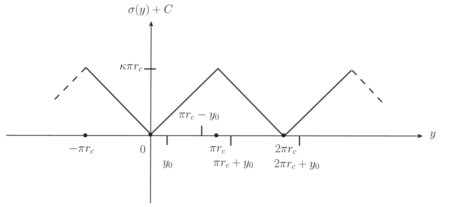
Figure 1: Warp function $\sigma(y)+C$ given by eq. (16).

The same is also true for our solution (16). At first site, $\sigma(y)$ becomes a constant outside the region $0\leqslant y\leqslant\pi r_{c}$. But it is not the case. Indeed, consider, for example, $y=\pi r_{c}+y_{0}$ with $0\leqslant y_{0}\leqslant\pi r_{c}$. Then we have the following sequence of equalities (for definiteness, in what follows $\kappa>0$):

$$\sigma(\pi r_{c}+y_{0})+C=\frac{\kappa}{2}(|y_{0}+\pi r_{c}|-|y_{0}|)+\frac{\kappa\pi r_{c}}{2}$$

$$=\frac{\kappa}{2}(|y_{0}+\pi r_{c}-\boldsymbol{2\pi r_{c}}|-|y_{0}|)+\frac{\kappa\pi r_{c}}{2}=\kappa(\pi r_{c}-y_{0})\;,$$ (43)

in accordance with fig. 1 and RS1 solution (41). Analogously, for $y=-y_{0}$ with $0\leqslant y_{0}\leqslant\pi r_{c}$,

$$\sigma(-y_{0})+C=\frac{\kappa}{2}(|-y_{0}|-|-y_{0}-\pi r_{c}|)+\frac{\kappa\pi r_{c}}{2}$$

$$=\frac{\kappa}{2}(|-y_{0}|-|-y_{0}-\pi r_{c}+\boldsymbol{2\pi r_{c}}|)+\frac{\kappa\pi r_{c}}{2}=\kappa y_{0}\;.$$ (44)

As it was already mentioned after eq. (19) the functions $\varepsilon(x)$ can be treated in a standard manner only for $0<|x|\leqslant\pi r_{c}$. Outside this region the periodicity condition should be imposed first. For instance, we obtain for $0<\epsilon<\pi r_{c}$

$$\int_{-\epsilon}^{\epsilon}dy\delta(y-\pi r_{c})=\frac{1}{2}[\varepsilon(\epsilon-\pi r_{c})-\varepsilon(-\epsilon-\pi r_{c})]$$

$$=\frac{1}{2}[\varepsilon(\epsilon-\pi r_{c})-\varepsilon(-\epsilon-\pi r_{c}+\boldsymbol{2\pi r_{c}})]=-1\;,$$ (45)

that results in

$$\int_{-\epsilon}^{\epsilon}dy\sigma^{\prime\prime}(y) =2\sigma^{\prime}(\epsilon)=\kappa\left[\lambda_{1}\!\!\int_{-\epsilon}^{\epsilon}dy\delta(y)+\lambda_{2}\!\!\int_{-\epsilon}^{\epsilon}dy\delta(y-\pi r_{c})\right]$$

$$=\kappa(\lambda_{1}-\lambda_{2})=2\kappa\;.$$ (46)

Thus, we get the correct result $\sigma^{\prime}(\epsilon)=\kappa$. Analogously, we find $\sigma^{\prime}(\pi r_{c}-\epsilon)=\kappa(\lambda_{1}-\lambda_{2})=\kappa$. The point $y=\epsilon$ ($y=\pi r_{c}-\epsilon$) lies in between the branes. That is why, $\sigma^{\prime}(\epsilon)$ ($\sigma^{\prime}(\pi r_{c}-\epsilon)$) is defined by both $\lambda_{1}$ and $\lambda_{2}$. This effect is one more manifestation of the symmetry with respect to the branes. Note that in the RS1 model $\sigma^{\prime}_{\mathrm{RS}}(\epsilon)$ is defined by one brane only, that requires $(\Lambda_{1})_{\mathrm{RS}}$ (25) to be twice as large as $\Lambda_{1}$ (23).

Starting from eq. (29), one can derive a compact expression for $\sigma^{\prime}(y)$. Let $y=y_{0}+(2k+1)$, where $0<y_{0}<\pi r_{c}$, $k=0,\pm 1,\ldots$. Since

$$\varepsilon(y_{0}+(2k+1)\pi r_{c}) =\varepsilon(y_{0}+(2k+1)\pi r_{c}-\boldsymbol{2(k+1)\pi r_{c}})=-1\;,$$

$$\varepsilon(y_{0}-\pi r_{c}+(2k+1)\pi r_{c}) =\varepsilon(y_{0}+2k\pi r_{c}-\boldsymbol{2k\pi r_{c}})=1\;,$$ (47)

we find that

$$\sigma^{\prime}(y_{0}+(2k+1)\pi r_{c})=\frac{\kappa}{2}(-\lambda_{1}+\lambda_{2})=-\kappa\;.$$ (48)

Analogously, we get for $y=y_{0}+2k\pi r_{c}$, $k=0,\pm 1,\ldots$,

$$\sigma^{\prime}(y_{0}+2k\pi r_{c})=\frac{\kappa}{2}(\lambda_{1}-\lambda_{2})=\kappa\;.$$ (49)

Two last formulas can be combined into a compact one ($y\neq n\pi r_{c}$, $n=0,\pm 1,\ldots$)

$$\sigma^{\prime}(y)=\kappa\,\varepsilon(\sin(y/r_{c}))\;.$$ (50)

Equation (50) results in relation $\sigma^{\prime}(-y)=-\sigma^{\prime}(y)$.

The $Z_{2}$ symmetry of $\sigma(y)$ can be shown as follows:

$$\sigma(-y) =\frac{\kappa}{2}(|-y|-|-y-\pi r_{c}|)+\frac{\kappa\pi r_{c}}{2}-C$$

$$=\frac{\kappa}{2}(|-y|-|-y-\pi r_{c}\boldsymbol{+2\pi r_{c}}|)+\frac{\kappa\pi r_{c}}{2}-C$$

$$=\frac{\kappa}{2}(|y|-|y-\pi r_{c}|)+\frac{\kappa\pi r_{c}}{2}-C=\sigma(y)\;.$$ (51)

The shift $\sigma(y)\rightarrow\sigma(y)-C$ is the change of four-dimensional part of the metric (1), namely

$$g_{\mu\nu}\rightarrow g_{\mu\nu}e^{2C}.$$ (52)

The Einstein tensor $R_{\mu\nu}-(1/2)g_{\mu\nu}R$ is invariant under such a transformation (remember that $C$ is a constant). As for the energy-momentum tensor, it is scale-invariant only for massless fields. For instance, the energy-momentum tensor of the massive scalar field,

$$T_{\mu\nu}=\partial_{\mu}\phi\,\partial_{\nu}\phi-\frac{1}{2}\,g_{\mu\nu}\!\left[g^{\alpha\beta}\partial_{\alpha}\!\phi\,\partial_{\beta}\phi-m^{2}\phi^{2}\right],$$ (53)

is not scale-invariant due to the third term in (53). In general, theories with massive fields are not invariant under transformation (52).

Consider the effective 4-dimensional gravity action on the TeV brane (with radion term omitted). It looks like (see, for instance, [15])

$$S_{\mathrm{eff}}=\frac{1}{4}\sum_{n=0}^{\infty}\int\!d^{4}x\!\left[\partial_{\mu}h^{(n)}_{\varrho\alpha}(x)\partial_{\nu}h^{(n)}_{\delta\lambda}(x)\,\eta^{\mu\nu}-m_{n}^{2}h^{(n)}_{\varrho\alpha}(x)h^{(n)}_{\delta\lambda}(x)\right]\!\eta^{\varrho\delta}\eta^{\alpha\lambda}\;.$$ (54)

The shift $\sigma(y)\rightarrow\sigma(y)-C$ can be also regarded as the rescaling of four-dimensional coordinates (see also [14])

$$x^{\mu}=e^{C}x^{\prime\mu}\;,$$ (55)

but then without change of the metric. Let us stress that (55) is not a particular case of general coordinate transformation in gravity, since the metric tensor $g_{\mu\nu}$ remains fixed.

The invariance of the action (54) under transformation (55) needs rescaling of the graviton fields and their mass: $h^{(n)}_{\mu\nu}=e^{-C}h^{\prime(n)}_{\mu\nu}$, $m_{n}=e^{-C}m^{\prime}_{n}$. We see that the theory of massive KK gravitons is not scale-invariant. Only its zero mass sector (standard gravity) remains unchanged.

Thus, one must conclude that warp functions $\sigma_{1}(y)$ and $\sigma_{2}(y)=\sigma_{1}(y)-C$ result in two non-equivalent 4-dimensional theories. As an illustration, the transition from the RS1 scenario to the RSSC scenario assumes the shift $\sigma(y)\rightarrow\sigma(y)-\pi\kappa r_{c}$. Correspondingly, the equation for the graviton masses in the RS1 model,

$$m_{n}\simeq x_{n}\kappa\,e^{-\kappa\pi r_{c}}\;,$$ (56)

transforms into equation in the RSSC model:

$$m^{\prime}_{n}\simeq m_{n}e^{\kappa\pi r_{c}}=x_{n}\kappa\;,$$ (57)

in accordance with the results of refs. [9]-[11], [14]-[15].

Recently, it was shown that an excess in the diphoton invariant mass spectrum seen in 13 TeV data at ATLAS [16] and CMS [17] is consistent with a warped compactification [18]-[22]. It particular, it was supposed [18] that the diphoton resonance at the LHC can be produced as follows:

$$pp\rightarrow h^{(1)}\rightarrow\gamma\gamma\;.$$ (58)

Here $h^{(1)}$ is the lowest graviton KK mode with the mass

$$m_{1}=x_{1}\kappa\;,$$ (59)

where $x_{1}=3.83$ is the first zero of the Bessel function $J_{1}(x)$. Thus, $\kappa=196$ GeV for $m_{1}=750$ GeV [18]. A comparison between (59), (38) shows that the physical framework used in [18] corresponds to the warped compactification scenario with $C=\kappa\pi r_{c}$ (for details, see Section 2).

In ref. [23] the $p_{\bot}$ distribution for the dielectron production at the LHC was calculated in such a scenario. By comparing theoretical predictions with the LHC data at 7 and 8 TeV, the following lower bound on $\bar{M}_{5}$ was obtained

$$\bar{M}_{5}>3.44\mathrm{\ TeV}\;.$$ (60)

Then for $C=\kappa\pi r_{c}$ we get from (39), (60):

$$\Lambda_{\pi}>14.4\mathrm{\ TeV}\;.$$ (61)

This inequality is not in contradiction with (although, not close to) the best-fit value $\Lambda_{\pi}\approx 60$ TeV obtained in [18].

It follows from eqs. (38), (39) that for any $C$

$$\frac{\bar{M}_{5}}{\kappa}=\left(\frac{\Lambda_{\pi}x_{1}}{m_{1}}\right)^{2/3}.$$ (62)

Putting $m_{1}=750$ GeV and $\Lambda_{\pi}=60$ TeV, we find

$$r=\left(\frac{\kappa}{\bar{M}_{5}}\right)^{3/2}\!\simeq 0.003\;.$$ (63)

The values of the parameters $\bar{M}_{5}$ and $\kappa$ taken separately depend on the particular RS-like scenario defined by the constant $C$. Let us put

$$C=a\kappa\pi r_{c}\;,$$ (64)

where $0<a<1$. Then we get from (30), (38):

$$\kappa=\bar{M}_{\mathrm{Pl}}\left(\frac{m_{1}}{x_{1}\bar{M}_{\mathrm{Pl}}}\right)^{a}\!\!r^{1-a}\;.$$ (65)

This equation results in $\kappa=0.003\bar{M}_{\mathrm{Pl}}$ for the RS1 scenario ($a=0$), and $\kappa=196$ GeV for the RSSC scheme ($a=1$). The gravity scale $\bar{M}_{5}$ is equal to $0.14\bar{M}_{\mathrm{Pl}}$, and 8.9 TeV, respectively.

4 Conclusions

To summarize, we have studied the space-time with non-factorizable geometry in four spatial dimensions with two branes (RS scenario). It has the warp factor $\exp[\sigma(y)]$ in front of four-dimensional metric. The generalization of the original RS solution of the Einstein-Hilbert equations for the function $\sigma(y)$ is obtained (16) which: (i) obeys the orbifold symmetry $y\rightarrow-y$; (ii) makes the jumps of $\sigma^{\prime}(y)$ on both branes; (iii) has the explicit symmetry with respect to the branes; (iv) includes the constant $C$ ($0\leqslant C\leqslant|\kappa|\pi r_{c}$). This constant can be used for model building within the framework of the general RS scenario.

Since our expression for $\sigma(y)$ is symmetric with respect to the brane positions, the brane tensions appeared to be the factor of two different than the RS1 tensions.

As a by-product, the compact analytical expression for $\sigma^{\prime}(y)$ is obtained (50).

It is worthy to note that an explicit expression which makes the jumps of $\sigma^{\prime}(y)$ on both branes was presented in [24],

$$\sigma_{\mathrm{DGGT}}(y)=\kappa\{y[2\,\theta(y)-1]-2(y-\pi r_{c})\,\theta(y-\pi r_{c})\}+\mathrm{constant}\;.$$ (66)

However, contrary to our formula (16), this expression is neither symmetric in variable $y$ nor invariant with respect to the interchange of the branes.

Some recent results related to the interpretation of the excess in the diphoton invariant mass spectrum at 13 TeV in terms of the warped compactification are briefly discussed.

References

• [1] L. Randall and R. Sundrum, Phys. Rev. Lett. 83 (1999) 3370 [hep-ph/9905221].
• [2] N. Arkani-Hamed, S. Dimopoulos and G. Dvali, Phys. Lett. B 429 (1998) 263 [hep-ph/9803315].
• [3] I. Antoniadis, N. Arkani-Hamed, S. Dimopoulos and G. Dvali, Phys. Lett. B 436 (1998) 257 [hep-ph/9804398].
• [4] N. Arkani-Hamed, S. Dimopoulos and G. Dvali, Phys. Rev. D 59 (1999) 086004 [hep-ph/9807344].
• [5] H. Davoudiasl, J.L. Hewett and T.G. Rizzo, Phys. Rev. Lett. 84 (2000) 2080 [hep-ph/9909255].
• [6] ATLAS Collaboration, New J. Phys. 15 (2013) 043007 [arXiv:1210.8389].
• [7] CMS Collaboration, Phys. Lett. B 720 (2013) 63 [arXiv:1212.6175].
• [8] A.V. Kisselev, Phys. Rev. D 88 (2013) 095012 [arXiv:1311.5316].
• [9] G. F. Giudice, T. Plehn and A. Strumia, Nucl. Phys. B 706 (2005) 455 [hep-ph/0408320].
• [10] A.V. Kisselev and V.A. Petrov, Phys. Rev. D 71 (2005) 124032 [hep-ph/0504203].
• [11] A.V. Kisselev, Phys. Rev. D 73 (2006) 024007 [hep-th/0507145].
• [12] A.V. Kisselev, JHEP 09 (2008) 039 [arXiv:0804.3941].
• [13] A.V. Kisselev, JHEP 04 (2013) 025 [arXiv:1210.3238].
• [14] V.A. Rubakov, Phys. Usp. 44 (2001) 871 [hep-ph/0104152].
• [15] E.E. Boos, Yu.A. Kubyshin, M.N. Smolyakov and I.P. Volobuev, Class. Quant. Grav. 19 (2002) 4591 [hep-th/0202009].
• [16] The ATLAS collaboration, Search for resonances decaying to photon pairs in 3.2 fb-1 of $pp$ collisions at $\sqrt{s}=13$ TeV with the ATLAS detector, ATLAS-CONF-2015-081.
• [17] The CMS collaboration, Search for new physics in high mass diphoton events in proton-proton collisions at 13 TeV, CMS-PAS-EXO-15-004.
• [18] S.B. Giddings and H. Zhang, Kaluza-Klein graviton phenomenology for warped compactification, and the 750 GeV diphoton excess, arXiv: 1602.02793.
• [19] C. Csáki and L. Randall, A Diphoton Resonance from Bulk RS, arXiv: 1603.07303.
• [20] J.L. Hewett and T.G. Rizzo, 750 GeV Diphoton Resonance in Warped Geometries, arXiv: 1603.08250.
• [21] A. Carmona, A 750 graviton from holographic composite dark sectors, arXiv: 1603.08913.
• [22] B.M. Dillon and V. Sanz, A Little KK Graviton at 750 GeV, arXiv: 1603.09550.
• [23] A.V. Kisselev, Particles and Nuclei, Letters 11 (2014) 1112 [arXiv: 1306.5402].
• [24] D. Dominici, B. Grzadkowski, J.F. Gunion and M. Toharia, Nucl. Phys. B 671 (2003) 243 [hep-ph/0206192].