Saturation of the magnetorotational instability in the unstratified shearing box with zero net flux: convergence in taller boxes

Abstract

Previous studies of the nonlinear regime of the magnetorotational instability in one particular type of shearing box model – unstratified with no net magnetic flux – find that without explicit dissipation (viscosity and resistivity) the saturation amplitude decreases with increasing numerical resolution. We show that this result is strongly dependent on the vertical aspect ratio of the computational domain $L_{\rm{z}}/L_{\rm{x}}$. When $L_{\rm{z}}/L_{\rm{x}}\lesssim 1$, we recover previous results. However, when the vertical domain is extended $L_{\rm{z}}/L_{\rm{x}}\gtrsim 2.5$, we find the saturation level of the stress is greatly increased (giving a ratio of stress to pressure $\alpha\gtrsim 0.1$), and moreover the results are independent of numerical resolution. Consistent with previous results, we find that saturation of the MRI in this regime is controlled by a cyclic dynamo which generates patches of strong toroidal field that switches sign on scales of $L_{\rm{x}}$ in the vertical direction. We speculate that when $L_{\rm{z}}/L_{\rm{x}}\lesssim 1$, the dynamo is inhibited by the small size of the vertical domain, leading to the puzzling dependence of saturation amplitude on resolution. We show that previous toy models developed to explain the MRI dynamo are consistent with our results, and that the cyclic pattern of toroidal fields observed in stratified shearing box simulations (leading to the so-called butterfly diagram) may also be related. In tall boxes the saturation amplitude is insensitive to whether or not explicit dissipation is included in the calculations, at least for large magnetic Reynolds and Prandtl number. Finally, we show MRI turbulence in tall domains has a smaller critical $\rm{Pm}_{c}$, and an extended lifetime compared to $L_{\rm{z}}/L_{\rm{x}}\lesssim 1$ boxes.

1 INTRODUCTION

The local shearing box model has proved to be very useful for studying the non-linear regime of the magneto-rotational instability (MRI)(Hawley et al., 1995). It is useful to classify such models into four types, depending on whether or not the domain contains net magnetic flux, and whether or not the vertical component of gravity is included (producing a vertically stratified density profile). Generally speaking, the results of numerical simulations that explore three of these four types of shearing box models can be summarized as follows.

1. Unstratified shearing box simulations with net flux show sustained MHD turbulence and numerically converged values of the stress and angular momentum transport. The saturated stress-to-pressure ratio $\alpha$ varies widely ($\sim 10^{-3}$-$0.1$) depending on the net magnetic field strength (Hawley et al., 1995; Sano et al., 2004; Guan et al., 2009; Simon et al., 2009).

2. Vertically stratified shearing box simulations with no net flux also show strong MRI driven turbulence with typical $\alpha\sim 10^{-3}$-$10^{-2}$, as well as dynamo activity that leads to a quasi-periodic pattern of alternating toroidal field (Brandenburg et al., 1995; Stone et al., 1996; Gressel, 2010; Simon et al., 2013a). The stress is independent of numerical resolution (Shi et al., 2010; Davis et al., 2010), although recently Bodo et al. (2014) have claimed at very high resolution this may no longer be the case. Further investigation of this issue is required.

3. Vertically stratified shearing box simulations with net flux show a wide range of behavior depending on the field geometry and strength (Stone et al., 1996; Miller & Stone, 2000). For example, sustained turbulence is observed with weak toroidal fields, while powerful outflows that depend on the field strength are produced in the case of net vertical fields, and the disk can show complex interplay between MRI and buoyancy (Parker) instabilities for strong toroidal fields (Suzuki & Inutsuka, 2009; Guan & Gammie, 2011; Simon et al., 2011; Fromang et al., 2013; Lesur et al., 2013; Bai & Stone, 2013a; Simon et al., 2013b).

The final case of an unstratified shearing box with no magnetic flux, introduced by Hawley et al. (1996) to study the MHD dynamo driven by the MRI, shows intriguing behavior. In this case simulations find that the saturated level of stress decreases as the numerical resolution is increased(Fromang & Papaloizou, 2007; Simon et al., 2009; Guan et al., 2009; Bodo et al., 2011). When physical dissipation (viscosity and resistivity) is included in the model, convergence of the stress with resolution is recovered(Fromang et al., 2007). Numerous works have also shown that the ratio of these two dissipation length scales seems to control the saturation level of stress driven by MRI turbulence (Fromang et al., 2007; Simon et al., 2009; Fromang, 2010), even when net flux is included (Lesur & Longaretti, 2007; Simon & Hawley, 2009; Meheut et al., 2015).

Since the important work of Fromang & Papaloizou (2007) there has been significant effort to investigate MHD dynamo action in the special case of unstratified no-net flux shearing box. Almost all of this work is based on spectral methods, so that explicit dissipation (both viscosity and resistivity) must be included. For example, Lesur & Ogilvie (2008b) found that long-lived cyclic dynamo activity occurs in an incompressible MHD model in which the aspect ratio of the computational domain is $(L_{\rm{x}}:L_{\rm{y}}:L_{\rm{z}})=(1:4:2)$, and these authors developed a toy dynamical model to explain the cycles. More recently, the work of Rincon et al. (2007); Rincon et al. (2008) has explored the subcritical dynamo mechanism in more detail, and in particular the role of the magnetic Prandtl number (ratio of viscosity to resistivity) in determining the outcome. Recent work (Riols et al., 2013, 2015) reveals the nonlinear dynamics of the MRI dynamo is more complex than expected.

Despite this progress, the question remains why, in compressible MHD with no explicit dissipation, does the saturation amplitude of the MRI depend so strongly on resolution? One hint may come from the extended vertical domain used in the study of MRI dynamos in incompressible MHD, e.g. Lesur & Ogilvie (2008b). Most previous studies in compressible MHD adopt a standard computational domain that spans one thermal scale height $H$ in the radial direction, and uses a vertical aspect ratio $L_{\rm{z}}/L_{\rm{x}}=1$ and a toroidal aspect ratio $L_{\rm{y}}/L_{\rm{x}}\gtrsim 4$. In contrast, studies of shear-driven dynamos have found that a large vertical aspect ratio is required for vigorous dynamo action (Yousef et al., 2008), consistent with the results of Lesur & Ogilvie (2008b).

In this work, we present new studies of the saturation of the MRI in compressible MHD in the no-net flux unstratified shearing box, both with and without explicit dissipation, to investigate the role of the size and aspect ratio of the computational domain on the results. Similar to the results reported in incompressible MHD, we find qualitatively different behavior when the vertical aspect ratio of the domain is large, $L_{\rm{z}}/L_{\rm{x}}\gtrsim 2.5$. In such case vigorous dynamo action produces a strong, cyclic toroidal magnetic field that greatly increases the level of turbulence and stress. Moreover the saturation amplitude of the turbulence is independent of numerical resolution, and independent of whether explicit dissipation is included in the model (at least for large magnetic Reynolds numbers and magnetic Prandtl numbers greater than one).

In reality, the unstratified shearing box with no net flux has very little relevance for real astrophysical disks, because it is impossible for each local patch in a global disk to maintain zero-net-flux for all time. Even if overall the disk has no net flux, large scale field loops on the scale of the vertical size of the disk will impart smaller local patches with a time-varying net flux. Moreover, in many astrophysical plasmas the dominant non-ideal MHD effect is not simply Ohmic dissipation, but rather ambipolar diffusion and/or the Hall effect (Wardle, 1999; Salmeron & Wardle, 2003). Significant progress has been made recently on investigating the role of ambipolar diffusion (Hawley & Stone, 1998; Bai & Stone, 2011, 2013b; Simon et al., 2013a, b) and the Hall effect (Sano & Stone, 2002; Kunz & Lesur, 2013; Lesur et al., 2014; Bai, 2014, 2015) on the saturation of the MRI in all four kinds of shearing box models described earlier, and the results differ significantly from models which include only Ohmic resistivity. Nevertheless, it is of interest to understand dynamo action in the unstratified no net flux shearing box (with and without resistivity) if only because it represents such a simple well-posed model. In addition, we show in this paper that the cyclic dynamo action observed in stratified shearing box models (resulting in the so-called butterfly diagram of toroidal field) may be related to that observed in more realistic unstratified domains.

The structure of the paper is as follows: we first describe the equations we solve and the numerical methods adopted in section 2; the main results are then presented in section 3; a short discussion of the dynamo action observed in our results follows in section 4; and finally in section 5 we summarize and conclude.

2 METHODS

2.1 Equations solved and code description

We solve the comprssible MHD equations adopting the “shearing box” approximation. In a Cartesian reference frame corotating with the disk at fixed orbital frequency $\Omega\hat{\mathbf{z}}$, the equations solved are as follows:

$$\frac{\partial\rho}{\partial t}+\nabla\cdot(\rho\mathbf{v})=0\,,$$ (1)

$$\frac{\partial\rho\mathbf{v}}{\partial t}+\nabla\cdot\left(\rho\mathbf{v}\mathbf{v}+\mathbf{T}\right)=-2\rho\Omega\hat{\mathbf{z}}\times\mathbf{v}+2q\rho\Omega^{2}x\hat{\mathbf{x}}\,,$$ (2)

$$\frac{\partial\mathbf{B}}{\partial t}-\nabla\times\left(\mathbf{v}\times\mathbf{B}\,-\,\eta\nabla\times\mathbf{B}\right)=0\,,$$ (3)

where $\hat{\mathbf{x}}$ refers to the radial direction, $\rho$ is the mass density, $\mathbf{v}$ is the velocity, $q=3/2$ is the Keplerian shear parameter, $\mathbf{B}$ is the magnetic strength, and $\eta$ is the Ohmic resistivity. The total stress tensor $\mathbf{T}$ is defined as

$$\mathbf{T}=\left(P+\frac{\mathbf{B}\cdot\mathbf{B}}{8\pi}\right)\mathbf{I}-\frac{\mathbf{B}\mathbf{B}}{4\pi}\,-\,\mathbf{\Pi}\,,$$ (4)

where $\mathbf{I}$ is the identity tensor, $P=\rho c_{\rm{s}}^{2}$ is the gas pressure, and $c_{\rm{s}}$ is the isothermal sound speed. The viscous stress $\mathbf{\Pi}$ can be expanded as

$$\Pi_{ij}=\rho\nu\left(\frac{\partial v_{i}}{\partial x_{j}}+\frac{\partial v_{j}}{\partial x_{j}}-\frac{2}{3}\delta_{ij}\nabla\cdot\mathbf{v}\right)\,,$$ (5)

where $\nu$ is the kinematic viscosity. Note that in Equation (2), the vertical tidal acceleration $\Omega^{2}z\hat{\mathbf{z}}$ is omitted, that is we are studying the unstratified shearing box. We include explicit viscosity and resistivity terms in some of our calculations, as discussed in section 3.5. However, in order to investigate the convergence of stress with numerical resolution without dissipation, most of simulations are ideal MHD.

We use the Athena (Stone et al., 2008; Stone & Gardiner, 2010) MHD code for our numerical simulations. We adopt the CTU integrator, third-order piecewise parabolic reconstruction with characteristic tracing in the primitive variables, and the Roe Riemann solver as the basic algorithms. The orbital advection scheme is used to increase the efficiency of calculation (Masset, 2000; Johnson et al., 2008). As the shearing box boundary conditions can cause mismatch of the integral of fluxes over the two radial faces due to remap (Gressel & Ziegler, 2007), using orbital advection can reduce this mismatch and improve the conservation (Stone & Gardiner, 2010). We ensure the conservation of vertical magnetic flux to machine precision by treating the shearing box boundary conditions carefully with a remapping method described in Stone & Gardiner (2010, Section 4).

2.2 Initial conditions and run setup

We initialize the disk density with a uniform distribution $\rho=\rho_{0}=1$ within the box. We set the unit of time $\Omega^{-1}=1$ and the unit of length $H=c_{\rm{s}}/\Omega=1$, and therefore the sound speed $c_{\rm{s}}$ and initial gas pressure $P_{0}=\rho_{0}c_{\rm{s}}^{2}$ are unity as well. The initial magnetic field is $\mathbf{B}=B_{0}\sin(2\pi x/L_{\rm{x}})\hat{\mathbf{z}}$, where $B_{0}$ is specified through the plasma $\beta_{0}\equiv P_{0}/(B_{0}^{2}/8\pi)=100$ for all runs. With this configuration, the net magnetic flux is zero in all three directions. We also ran several models in which the initial magnetic field geometry and strength were varied to check that our results do not depend on the precise form of the initial conditions, provided the net flux is zero. We adopt periodic boundary conditions in the azimuthal ($y$) and vertical ($z$) directions, and shearing periodic in the radial ($x$) direction (Hawley et al., 1995).

We carry out multiple sets of simulations with various box sizes $L_{\rm{x}}\in\{0.25,0.5,1.0\}\,H$, vertical to radial aspect ratios $L_{\rm{z}}/L_{\rm{x}}=0.5$-$12$ and numerical resolutions $(\Delta x)^{-1}=(\Delta y)^{-1}=(\Delta z)^{-1}\in\{32,64,128,256\}\,H^{-1}$. Parameters for all our runs are all listed in Table 1. We do not vary the toroidal aspect ratio $L_{\rm{y}}/L_{\rm{x}}$ in this work, instead we fix $L_{\rm{y}}/L_{\rm{x}}=4$ for all runs. Provided $L_{\rm{y}}/L_{\rm{x}}\gtrsim 1$, it has been found that different sized domains in the toroidal direction primarily affect the spectrum and amplitude of spiral density waves excited by the turbulence and amplified by shear Heinemann & Papaloizou (2009), however such waves do not dominate the saturation level of stress.

2.3 Diagnostics

In order to facilitate analysis and obtain statistical properties of our simulations, we define a few ways to average physical variables. We first define a volume (box) average:

$$\langle X\rangle\equiv\frac{\int\,X\,dxdydz}{\int dxdydz}\,.$$ (6)

We also define a time average

$$\langle X\rangle_{t}\equiv\frac{\int\,X\,dt}{\int dt}\,.$$ (7)

The time average is generally applied over $\sim 200$ orbits to eliminate chaotic fluctuations and achieve meaningful statistics (Winters et al., 2003). Using these averages, we write the time averaged Maxwell and Reynolds stresses as

$$\alpha_{\rm M}\equiv\langle\langle-\frac{B_{\rm{x}}B_{\rm{y}}}{4\pi P_{0}}\rangle\rangle_{t}\,,~{}\alpha_{\rm R}\equiv\langle\langle\frac{\rho v_{x}\delta v_{y}}{P_{0}}\rangle\rangle_{t}$$ (8)

respectively. In Table 1 we also list the total internal stress, $\alpha_{\rm tot}\equiv\alpha_{\rm R}+\alpha_{\rm M}$. We use these stresses as a measure of the saturated level of MRI turbulence throughout this paper.

As some of our simulations develop large scale coherent field structures within the box, we therefore introduce a horizontal average:

$$\overline{X}\equiv\frac{\int\,X\,dxdy}{\int dxdy}\,.$$ (9)

This average is useful for decomposing the total magnetic field $\mathbf{B}$ into mean and fluctuating parts. i.e.

$$\mathbf{B}=\overline{\mathbf{B}}+\mathbf{b}\,,$$ (10)

where $\mathbf{b}$ denotes the turbulent (small scale) fluctuating field.

3 RESULTS

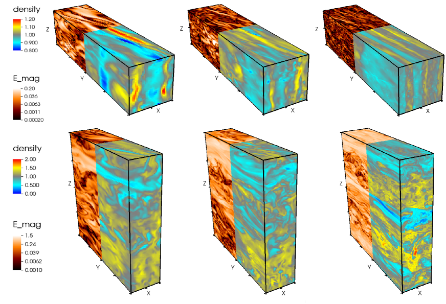
Figure 1: Snapshots (at $t=150$ orbits) from standard box (top row, $L_{\rm{x}}=L_{\rm{y}}/4=L_{\rm{z}}=1\,H$) and tall box (bottom row, $L_{\rm{x}}=L_{\rm{y}}/4=L_{\rm{z}}/4=1\,H$) simulations. Shown in each case are magnetic energy (far half) and density (near half) distributions. From left to right, the resolution is $32/H$, $64/H$, and $128/H$. Turbulence becomes weaker in the standard box case as resolution increases; while it maintains constant amplitude in the tall box runs. Note the color scale of the magnetic energy is logarithmic, and the color bars in the bottom and top rows are different.

3.1 Saturation in tall versus short boxes

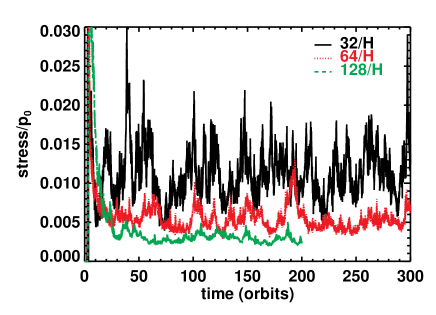
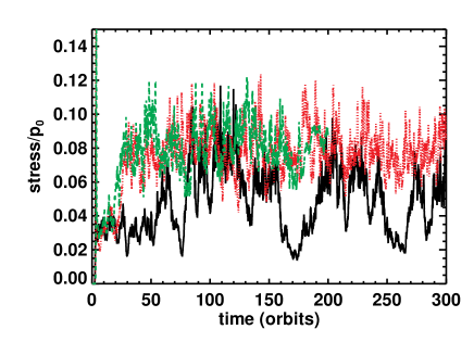
Figure 2: The volume averaged stresses for a standard box ($(L_{\rm{x}},L_{\rm{y}},L_{\rm{z}})=(1,4,1)\,H$, left panel) and a tall box ($(L_{\rm{x}},L_{\rm{y}},L_{\rm{z}})=(1,4,4)\,H$, right) with various resolutions: $32/H$(black solid),$64/H$(red dotted) and $128/H$(green dashed). In contrast to the small box, the vertically elongated box achieves good convergence.

We begin by studying saturation in the standard computational domain, $(L_{\rm{x}},L_{\rm{y}},L_{\rm{z}})=(1,4,1)\,H$. We begin with a numerical resolution of $32/H$. We refer to this simulation as x1y4z1r32, where our naming convention gives both the box dimensions (in $H$) and resolution. We then double this resolution twice (simulations x1y4z1r64 and x1y4z1r128) to reproduce previous results. The top panels of Figure 1 show 3D snapshots of the magnetic energy and density in these runs. As the resolution improves from left to right, the magnetic energy is reduced, and turbulence becomes weaker. At the highest resolution (x1y4z1r128 in the right panel) the density field is dominated by $k_{\rm z}=0$ shearing waves (Heinemann & Papaloizou, 2009), and there is little indication of turbulence.

We then repeat these runs in a taller box, $(L_{\rm{x}},L_{\rm{y}},L_{\rm{z}})=(1,4,4)\,H$, varying the resolution from $32/H$ for run x1y4z4r32, to $64/H$ for run x1y4z4r64, and to $128/H$ for run x1y4z4r128. Snapshots of magnetic energy and density for these runs are shown in the bottom row of Figure 1. In contrast to the standard box case, we see no signs of weakening turbulence as resolution improves from left to right. The typical magnetic energy rises slightly from x1y4z4r32 to x1y4z4r64, and stays roughly at the same level as the resolution doubles again in x1y4z4r128. The typical density fluctuation follows the similar trend, and are dominated by small scale turbulent fluctuations. At the same time, both the density and magnetic field show a large amplitude vertical mode with wavelength about half the vertical size of the box.

To quantify the resolution effects, we measure the volume averaged total stress $\alpha_{\rm tot}$ (the sum of the Maxwell and Reynolds stresses normalized with thermal pressure defined in section 2.3) and the results are shown in Figure 2. In the standard box runs (the top left panel), after a short transient growth ($\sim 30$ orbits), the total stresses reaches a quasi-steady state that last hundreds of orbits through the end of the simulations. The time-averaged stresses are therefore well defined and are measured over the last $100$-$200$ orbits (see Table-1 for the exact number used for averages). Comparing the saturation levels at different resolutions, we confirm the stress decreases as the resolution improves, roughly by a factor of two every time the resolution is doubled. In particular, $\alpha_{\rm tot}$ drops from $10^{-3}$ for x1y4z1r32 to $5\times 10^{-4}$ when the resolution is doubled, and drops by another factor of $\sim 2$ when $128/H$ is used. This behavior is identical to that previously reported (e.g., Fromang & Papaloizou, 2007; Simon et al., 2009; Guan et al., 2009; Bodo et al., 2011).

Remarkably, the decrease in stress with resolution that appears in the standard box is not reproduced in the taller box simulations. In the bottom left panel of Figure 2, we show that the volume averaged stress does in fact converge with numerical resolution for runs x1y4z4r32 through x1y4z4r128. In these cases, $\alpha_{\rm tot}\simeq 0.08$ is reached once the resolution exceeds $32/H$.

Figure  2 also demonstrates that the amplitude of the converged stress in the tall box is significantly greater than those in the standard domain. For example, the time averaged $\alpha_{\rm tot}\simeq 0.079$ in x1y4z4r64, almost $15$ times larger than $\alpha_{\rm tot}\simeq 0.005$ in x1y4z1r64, while $\alpha_{\rm tot}\simeq 0.08$ in x1y4z4r128, some $\sim 30$ times greater than that of x1y4z1r128. The magnetic energy in simulations performed in the tall box is also much greater than in the standard box runs; typically $\langle B^{2}/8\pi P_{0}\rangle\simeq 0.27$ which is a factor of $\gtrsim 50$ time bigger (this is also evident in Figure 1 where different color scales must be used for the two cases). The large values of the stress achieved in taller boxes is also of interest in that they are close to the values inferred from observations suggesting that in fully ionized accretion disk (e.g. dwarf novae in outburst) $\alpha_{\rm tot}\sim 0.1$–$0.4$, alleviating some of the concerns raised by King et al. (2007) regarding the discrepancy between values suggested by observations and measured in simulations.

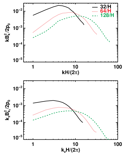
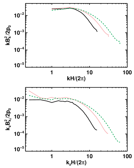
Figure 3: The power spectra of magnetic density energy for a standard box ($(L_{\rm{x}},L_{\rm{y}},L_{\rm{z}})=(1,4,1)\,H$, (left two panels) and a tall box ($(L_{\rm{x}},L_{\rm{y}},L_{\rm{z}})=(1,4,4)\,H$, right two panels) with various resolutions: $32/H$(black solid),$64/H$(red dotted) and $128/H$(green dashed), where $B_{k}^{2}$ is spherical shell integrated value and $B_{k_{z}}^{2}$ is integrated along constant $k_{z}$ plane. In contrast to the small box case, where the self-similar power spectra decays with resolution, it achieves good convergence at low wave number in the tall box.

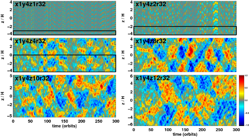
Figure 4: Space-time diagrams of the horizontally averaged azimuthal field $\overline{B}_{y}$ for various runs as labeled. Runs with $L_{\rm{z}}<8\,H$ are duplicated $8$ (for x1y4z1r32), $4$ (for x1y4z2r32), and $2$ (for x1y4z4r32) times, so that the images have the same aspect ratio of run x1y4z8r32. The individual black box shows the actual box we simulate. Large and structured azimuthal B-field appears when $L_{\rm{z}}>2\,H$.

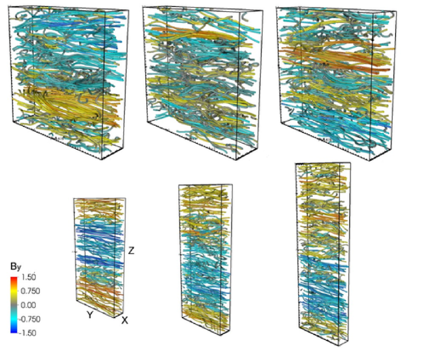
Figure 5: Top row: large scale magnetic field in x1y4z4r32 run reverses between $t=200$ orbits (top left) and $220$ orbits (top right); $t=210$ at the middle show more tangled field during this transition. Bottom row: snapshots of large scale field structures in other tall box runs (x1y4z8r32, x1y4z10r32, and x1y4z12r32 from left to right). In all panels, tubes are field lines in the box with starting points randomly distributed; color bar describes the value of $B_{y}/\sqrt{4\pi\rho_{0}}c_{\rm{s}}$ to show the orientation and strength of magnetic field in azimuth.

Further important insights into the differences between the saturated state in standard and tall boxes are revealed by the Fourier power spectrum. The right column of Figure 3 shows the magnetic energy density power spectra calculated over either spherical shells of constant $k$ ($kB_{k}^{2}$) or along a constant $k_{z}$ plane ($k_{z}B_{k_{z}}^{2}$) for both the standard (left) and tall box (right). The definition of both can be find in Davis et al. (2010, section 2.1). The spectra in the standard box peak at an intermediate wavenumber that increases with the resolution, and with an overall amplitude that decreases with resolution (but with a shape that is unchanged). In stark contrast, however, in the tall box the power spectra peak (or plateau) at the lowest wavenumbers ($k\sim 1$-$5$) at all resolutions. Such spectra are much more reminiscent of turbulence driven at a large outer scale, with an energy cascade to high $k$ independent of numerical resolution. These spectra suggest there is a resolved characteristic outer length scale in the tall box simulations. We note the spectrum and its dependence on resolutions of those tall box runs are also very different than those using standard short boxes with explicit dissipation (e.g., Figure 3 in Fromang, 2010) due to the lack of a large scale dynamo in the short boxes. However, a large scale dynamo, as we will show in the next subsection, is present in our tall box simulations.

3.2 A large scale dynamo

The images of magnetic energy and density shown in Figure 1, and the power spectra in Figure 3, both indicate that large-amplitude and large-scale vertical structure appears in simulations in tall boxes. In this section, we show this structure is associated with a large scale dynamo action that is triggered in the vertically extended box. Figure 4 plots a space-time diagram of the horizontally averaged azimuthal magnetic field in both standard and tall boxes. Patches of strong $\overline{B}_{y}$ that extend over vertical regions of size $\sim H$ are evident in run x1y4z4r32, with the sign of the field alternating quasi-periodically over $\sim 10$-$20$ orbits. The pattern become even more clear in the panels corresponding to runs x1y4z8r32, x1y4z10r32 and x1y4z12r32 (see especially the middle right panel in Figure 4). Clearly, a large scale dynamo must be operating that generates such strong ordered toroidal field. The 3D structure of the magnetic field at three different times during one reversal cycle in run x1y4z4r32 is explored further in Figure 5. Large scale ($k_{x}=k_{y}=0$ and $k_{z}=1$) patterns in the azimuthal magnetic field form along the azimuthal direction. Spatially, the field lines flip signs (from red to blue) with height to conserve the zero-net-flux initial condition. Their orientations also reverse from one state of coherent structures (top left at $t=200$ orbits) to another (top right at $t=220$ orbits). This result is similar to the dynamo cycle reported in Lesur & Ogilvie (2008b) (see their Figure 3). However, we emphasize that no explicit dissipation (viscosity or resistivity) is required to capture the dynamo, nor is it required to see a converged level of stress.

The large scale dynamo maintains a time averaged mean field $\langle\langle\overline{B}^{2}/8\pi P_{0}\rangle\rangle_{t}\simeq 0.06$ for x1y4z4r32 and $\simeq 0.13$ for x1y4z4r64 and x1y4z4r128 runs, which amount to $\sim 40$-$50\%$ of the total magnetic energy in the box (see Table 1 and  2), close to a state of equalized mean $\overline{\mathbf{B}}$ and turbulent ($\mathbf{b}$) field strength. In contrast, runs in the standard box do not exhibit strong cyclic dynamo behavior (see top left panel of Figure 4), and the mean field is rather weak, $\langle\langle\overline{B}^{2}/8\pi P_{0}\rangle\rangle_{t}\lesssim 0.1\langle\langle b^{2}/8\pi P_{0}\rangle\rangle_{t}$ for x1y4z1r32, and it drops further down to $\simeq 2\%$ of the turbulent magnetic energy in run x1y4z1r128.

Why does dynamo action produce a larger value for the stress which does not vary with numerical resolution? The large scale vertical patches of azimuthal magnetic field produced by the dynamo act locally as a region with net toroidal flux. Thus, each $L_{\rm{z}}\sim H$ patch acts as an unstratified shearing box with net toroidal field. As is already known, shearing boxes with net flux produce saturated stress which is independent of resolution (Guan et al., 2009; Simon & Hawley, 2009). As a result of (locally) strong magnetic field, the saturated Maxwell stress in x1y4z4r128 is $\alpha_{\rm M}\simeq 0.0714$, $\sim 31\times$ greater than that of x1y4z1r128. Of this total, $\sim 16\%$ is due to the correlated mean field $-\overline{B}_{x}\overline{B}_{y}/4\pi$, while the majority is still from the correlation between the perturbed field components $-b_{x}b_{y}/4\pi$ (since $\overline{B}_{x}$ is still small). In contrast, in the standard-sized box almost all of the stress is associated with the perturbed field.

We find the stress-to-energy ratio, $\alpha_{\rm mag}\equiv\langle\langle-2B_{x}B_{y}\rangle\rangle_{t}/\langle\langle B^{2}\rangle\rangle_{t}\simeq 0.27$ in the tall box, smaller than in the standard box case in which $\alpha_{\rm mag}\simeq 0.46$. A diminished $\alpha_{\rm mag}$ is also observed in simulations with strong net azimuthal flux (run Y8 in Hawley et al., 1995), where the imposed azimuthal mean field resembles a subsection of our box which contains $\overline{B}_{y}$ of the same sign.

3.3 Varying the aspect ratio $L_{\rm{z}}/L_{\rm{x}}$: a parameter survey

We now investigate the effect of varying the aspect ratio using $L_{\rm{z}}/L_{\rm{x}}\in\{0.5,1,2,2.5,3,3.5,4,6,8,10,12\}$ with fixed size $L_{\rm{y}}=4H$ and $L_{\rm{x}}=H$ in the horizontal dimensions. For each of $L_{\rm{z}}/L_{\rm{x}}$, we also vary the resolution to study numerical convergence. We first plot the $\alpha_{\rm tot}$ in Figure 6. This figure clearly demonstrates what may be our most important result. The data falls into two groups which show distinctly different behavior; the two groups are separated by the vertical dashed line at $L_{\rm{z}}/L_{\rm{x}}\simeq 2.5$. For aspect ratios $\lesssim 2.5$ (to the left of the dotted line), the stress decays linearly with the vertical size $L_{\rm{z}}$. Moreover, at any given aspect ratio, the stress decreases with increasing numerical resolution as shown by the decreasing amplitude of the black ($32/H$), red ($64/H$) and green ($128/H$) points. Clearly the standard box, with $L_{\rm{z}}/L_{\rm{x}}=1$ falls in this group. In contrast, for aspect ratios $L_{\rm{z}}/L_{\rm{x}}\gtrsim 2.5$ (to the right of the dotted line), the saturated stress associated with MRI turbulence appears independent of the vertical size $L_{\rm{z}}$, approaching $\alpha_{\rm tot}\sim 0.1$. Moreover, numerical convergence in the value of the stress is achieved for aspect ratios $L_{\rm{z}}/L_{\rm{x}}>4$. For example, for $L_{\rm{z}}/L_{\rm{x}}=8$, the stress values are nearly identical for resolutions of $32/H$ through $128/H$. The behavior of the two groups in this figure simply reflect the emergence of dynamo action in runs with a large vertical extent, which controls the stress. For example, the $L_{\rm{z}}/L_{\rm{x}}=4$, $8$, $10$, and $12$ cases in Figure 4 and 5 show strong cyclic azimuthal magnetic field driven by the underlying dynamo mechanism.

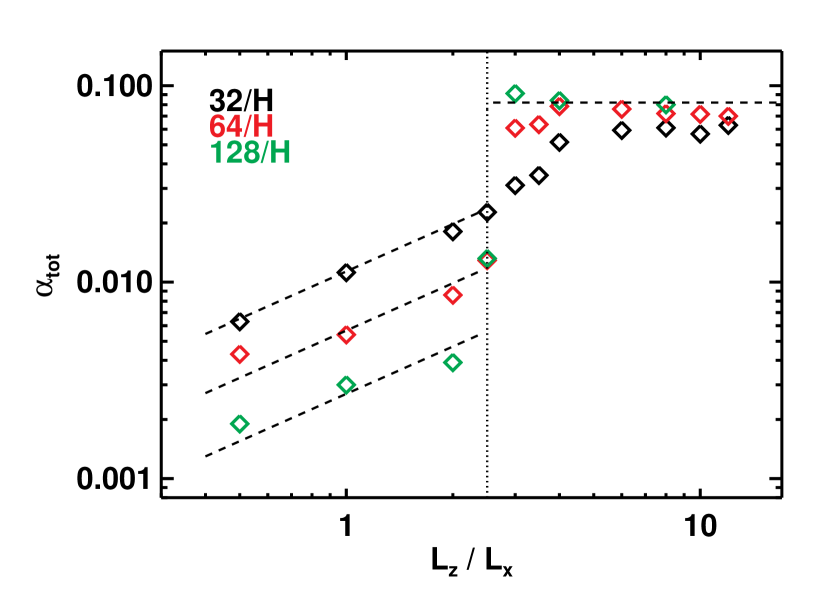
Figure 6: The sum of Maxwell and Reynolds stress for various aspect ratios ($L_{\rm{z}}/L_{\rm{x}}$) and resolutions for $L_{\rm{x}}=L_{\rm{y}}/4=1\,H$ boxes. The vertical dotted line separates the ‘diverging’ and ‘converging’ regions: to the left of this line, the stress decays with increasing resolution; the stress converges to $\sim 0.08$ for different $L_{\rm{z}}/L_{\rm{x}}$ on the right.

For all runs, the Maxwell stress dominates the total turbulent angular momentum transport; the ratio of the Maxwell to the Reynolds stress varies with different $L_{\rm{z}}/L_{\rm{x}}$ in a similar way (but at reduced amplitude) as the $\alpha_{\rm tot}$. In Figure 7, we find $\alpha_{\rm M}/\alpha_{\rm R}$ rises gradually from $\sim 3$ to $4$ as $L_{\rm{z}}/L_{\rm{x}}$ is increased from $0.5$ to $2$. The ratio then levels off, ranging between $4$ and $6$. This is greater than the typical values previously reported in the literature with Keplerian shear ($\sim 3$-$4$) (Hawley et al., 1995; Abramowicz et al., 1996; Stone et al., 1996; Hawley et al., 1999; Sano et al., 2004; Pessah et al., 2006). As the strong coherent field structures tend to eliminate strong velocity fluctuations and therefore reduce the Reynolds stress in those regions (similar to those observed in the corona regions of stratified boxes (Brandenburg et al., 1995; Miller & Stone, 2000)), the box averaged $\alpha_{\rm M}/\alpha_{\rm R}$ therefore rises above the previously reported values.

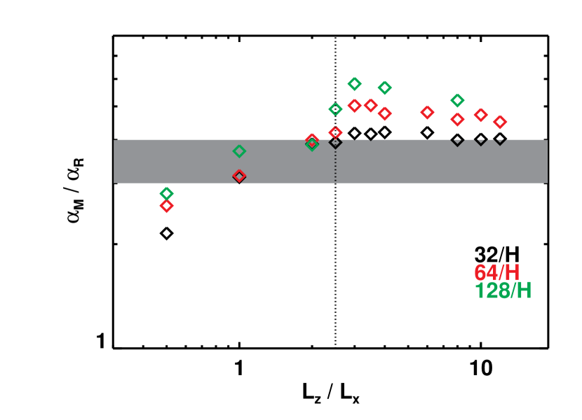
Figure 7: The ratio of the Maxwell stress and the Reynolds stress as a function of $L_{\rm{z}}/L_{\rm{x}}$ and numerical resolution. The vertical dotted line at $L_{\rm{z}}/L_{\rm{x}}=2.5$ same as Figure 6. The Maxwell stress always dominates the Reynolds in all runs; the ratio increases by a factor of $\sim 2$ in the small box regime, while stays roughly constant in the tall box cases. The tall box runs have greater $\alpha_{\rm M}/\alpha_{\rm R}$ than previous measurements marked as the shaded region.

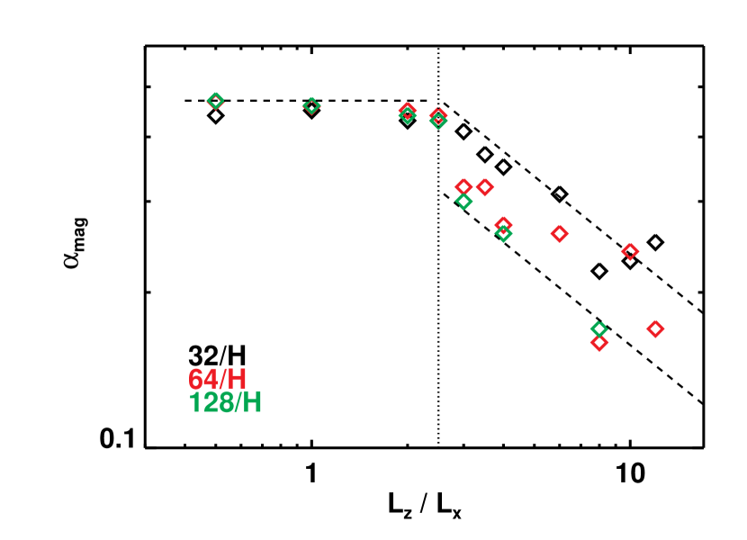
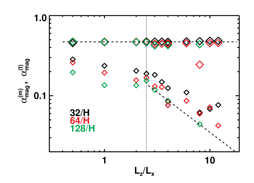
Figure 8: Top: $\alpha_{\rm mag}\equiv-2\langle\langle B_{x}B_{y}\rangle\rangle_{t}/\langle\langle B^{2}\rangle\rangle_{t}$ for various $L_{\rm{z}}/L_{\rm{x}}$ and resolutions. Again, the vertical dotted line delineates the short and tall box regimes. The horizontal dashed line shows that $\alpha_{\rm mag}$ stays constant in the small box regime; the dashed lines at $L_{\rm{z}}/L_{\rm{x}}>2.5$ follows the $(L_{\rm{z}}/L_{\rm{x}})^{-1/2}$ power law. Bottom: stress-to-energy ratios computed with pure mean field (small symbols) and turbulent field (large symbols) as defined in 11. The turbulent ratio keeps constant $\alpha_{\rm mag}^{(t)}\sim 0.47$ (the horizontal dashed line); while its mean field counterpart $\alpha_{\rm mag}^{(m)}\propto(L_{\rm{z}}/L_{\rm{x}})^{-1}$ (the dashed line at $L_{\rm{z}}/L_{\rm{x}}>2.5$), much smaller than $\alpha_{\rm mag}^{(t)}$.

The ratio between the Maxwell stress and magnetic energy, $\alpha_{\rm mag}$ (see definition in section 3.2), is usually adopted as a measure of sufficient resolution to capture MRI turbulence (e.g., $\alpha_{\rm mag}=0.3-0.4$ in Blackman et al., 2008; Hawley et al., 2011). We find consistent results for our standard boxes ($L_{\rm{z}}/L_{\rm{x}}\lesssim 2.5$), in which a relatively constant $\alpha_{\rm mag}\sim 0.47$ is obtained, in spite of that no convergence is achieved for the stress. Surprisingly, this ratio falls with $(L_{\rm{z}}/L_{\rm{x}})^{-1/2}$ in our tall box runs where converged stresses are found. As the stress stays roughly constant in those tall boxes, it is the increase of magnetic energy (or $1/\beta$) as $(L_{\rm{z}}/L_{\rm{x}})^{1/2}$ that drives this scaling.

The dynamo effect in tall boxes alters the underlying magnetic field structure. As discussed in section 3.1, most of the stress comes from the correlation of the small scale field, and $\langle-B_{\rm{x}}B_{\rm{y}}\rangle\sim\langle-b_{\rm{x}}b_{\rm{y}}\rangle\gg\langle-\overline{B}_{\rm x}\overline{B}_{\rm y}\rangle$ holds true for both groups. However, the magnetic energy in smaller boxes is mostly from the azimuthal component of the turbulent field, i.e., $\langle B^{2}\rangle\sim\langle b_{\rm{y}}^{2}\rangle\gg\langle\overline{B}_{\rm y}^{2}\rangle$; while $\langle B^{2}\rangle\sim\langle\overline{B}_{\rm y}^{2}\rangle\gg\langle b_{\rm{y}}^{2}\rangle$ in tall boxes. As a result, $\alpha_{\rm mag}$ roughly measures $\left|b_{\rm{x}}/b_{\rm{y}}\right|$ in the standard box cases, but it traces a very different quantity, $\left|b_{\rm{x}}b_{\rm{y}}\right|/\overline{B}_{\rm y}^{2}$ in the tall boxes. The effects of increasing the aspect ratio in an already elongated box would only introduce a stronger mean magnetic field. For instance, we find the total magnetic energy rises from $\langle B^{2}/8\pi P_{0}\rangle\simeq 0.27$ to $0.37$ when comparing x1y4z4r128 and x1y4z8r128 in Table 2, and the energy increase mostly goes into $\langle\overline{B}_{\rm y}^{2}/8\pi P_{0}\rangle$ so that the latter increases from $\simeq 0.13$ to $0.25$ while the other magnetic field components stay constant.

In a recent review, Blackman & Nauman (2015) pointed out the stress-to-energy ratios for the pure mean and turbulent field could be different. Following their proposal, we define

$$\alpha_{\rm mag}^{(m)}\equiv-2\frac{\langle\overline{B}_{\rm x}\overline{B}_{\rm y}\rangle}{\langle\overline{B}^{2}\rangle}\,;\alpha_{\rm mag}^{(t)}\equiv\frac{-2\langle b_{\rm{x}}b_{\rm{y}}\rangle}{\langle B^{2}\rangle-\langle\overline{B}^{2}\rangle}$$ (11)

for the mean field and turbulent field respectively. In the bottom panel of Figure 8, we find the ratio of the turbulent field (larger symbols) still reaches a constant $\alpha_{\rm mag}^{(t)}\sim 0.47$, while the mean field counterpart $\alpha_{\rm mag}^{(m)}\ll\alpha_{\rm mag}^{(t)}$, and decreases linearly with $L_{\rm{z}}/L_{\rm{x}}$. These are consistent with the results found in Blackman & Nauman (2015).

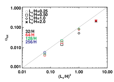
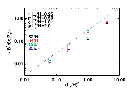
Figure 9: The box size dependence of the stress (left) and magnetic energy (right) for $L_{z}/L_{x}=4$ runs. We note that for both panels, the $x$-axes are $(L_{\rm{x}}/H)^{2}$ instead of $L_{\rm{x}}$. The dashed lines shows the $\propto(L_{x}/H)^{2}$ scaling. A strong linear correlation between the stress/energy and $(L_{\rm{x}}/H)^{2}$ is obtained which indicates a way to re-normalize $\alpha$ and $\langle B^{2}\rangle$ using the squared length scale $L_{\rm{x}}^{2}$.

3.4 Varying the box size with fixed aspect ratio

For given box size $L_{\rm{y}}=4H$, $L_{\rm{x}}=H$ in the horizontal domain, we find the stresses converge in the tall box runs ($L_{\rm{z}}/L_{\rm{x}}\gtrsim 2.5$) owing to the emergence of large scale azimuthal magnetic field produced by dynamo action that acts as a local non-zero net flux. Since the mean field sets an extra length scale that is directly related to the box size, it is also important to see how does the stress depend on the box size itself. Therefore we have performed an additional series of runs in which we vary $L_{\rm{x}}$, but keep the aspect ratio $L_{\rm{z}}/L_{\rm{x}}$ fixed.

In general, we find the amplitude of the saturated stress still converges to a constant value independent of numerical resolution as long as $L_{\rm{z}}/L_{\rm{x}}>2.5$ (see Table-1). However, the value to which the stress converges depends on the box size, as found previously for shearing box simulations with net azimuthal field (Hawley et al., 1995; Guan et al., 2009). As shown in Figure 9, both $\alpha_{\rm tot}$ and $\langle B^{2}/8\pi P_{0}\rangle$, measured from runs with aspect ratio of $1:4:4$ scale as $\propto L_{\rm{x}}^{2}$. This differs from the saturation predictor used in Hawley et al. (1995), in which a linear relation $\propto L_{\rm{y}}$ is reported. However, their relation applied to relatively weak ($\beta\sim O(10^{2})$) external azimuthal field is very different than the very strong ($\beta\sim O(10)$), dynamo generated oscillating azimuthal field observed in our runs.

In fact, the unstratified box does not have any intrinsic length scales other than the box size $L_{\rm{x}}$, cell width $\Delta x$, and (for compressible flows) the sonic scale $c_{s}/\Omega$. If we assume that compressible effects can be ignored (we return to this point below), then based on a dimensional analysis the stress can be normalized by $\rho_{0}(q\Omega L_{\rm{x}})^{2}$ (Fromang & Papaloizou, 2007; Guan et al., 2009), giving stress $\propto L_{\rm{x}}^{2}$ as reported above. As long as the simulation is resolved $L_{\rm{x}}/\Delta x\gtrsim 32$, we find negligible dependence of the stress on numerical resolution, e.g. Figure 9. We find similar scaling with size for other quantities such as magnetic and kinetic energy, and Reynolds stress. In addition, the scaling $\propto L_{\rm{x}}^{2}$ applies to runs using other values of the aspect ratio, e.g., $L_{\rm{z}}/L_{\rm{x}}=8$ as tabulated in Table 1.

In Figure 10, we plot the Fourier power spectra of five different runs computed with different numerical resolutions and physical box size (both $L_{\rm{x}}=H$ and $L_{\rm{x}}=0.5H$), but normalizing both the spectra and wavenumber according to the above scaling. Interestingly, all runs contain the same amplitude and slope at small $k$ (the “inertial range"), but extend to successively larger $k$ as the resolution is increased. Moreover, run x0.5y2z2r64 recovers the results of run x1y4z4r32 identically, and run x0.5y2z2r128 resembles x1y4z4r64 as well. Since these two pairs of runs have the same range of scales $L_{\rm{x}}/\Delta x$, we expect them to show similar behavior provided there are no intrinsic length scales in the model. The result clearly indicates that indeed the properties of MRI turbulence in the unstratified shearing box model depend only on dimensionless wavenumber $kL$. As a result, similar properties found in previous sections for tall boxes of $L_{\rm{x}}=H$ are also present in tall boxes with different $L_{\rm{x}}$.

Returning to Figure 9, the stress measured in our simulations deviates slightly from the $(L_{\rm{x}}/H)^{2}$ power law scaling at $\alpha\gtrsim 0.1$, which occurs in the largest boxes. We speculate this is due to compressibility effects (Sano et al., 2004). Such large values of $\alpha$ are associated with very strong (nearly sonic) turbulence. For example, the rms density fluctuation for runs with large $L_{\rm{x}}$ become as large as $\langle(\delta\rho/\rho_{0})^{2}\rangle^{1/2}\sim 0.25$ in x2y8z8r64. Compressibility strongly damps the turbulence, and prevents the turbulent magnetic field from growing even stronger. Obviously compressibility effects must play a role at some point, as turbulence alone cannot generate $\alpha\gg 1$.

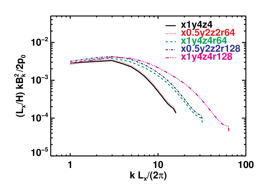
Figure 10: Rescaled magnetic energy power spectra for boxes with same aspect ratio $L_{\rm{z}}/L_{\rm{x}}=4$. The close matches between x1y4z4 and x0.5y2z2r64, x1y4z4r64 and x0.5y2z2r128 indicate that the underling turbulence is intrinsically the same but only rescaled to a different box size.

3.5 Explicit dissipation

Previous work has shown that if explicit dissipation is included in the unstratified shearing box model with no net flux using the standard box size $L_{\rm{z}}/L_{\rm{x}}=1$, then a converged value for the magnetic stress can be achieved (Fromang et al., 2007). The saturation level of the stress in this case is highly sensitive to the magnetic Prandtl number $\rm{Pm}$. It increases almost linearly with $\rm{Pm}$ in the range $4\leq\rm{Pm}\leq 16$; while turbulence is completely suppressed once the magnetic Prandtl number is below some critical value $\rm{Pm}_{c}\sim 2$-$4$ (Fromang et al., 2007; Simon & Hawley, 2009). Further study suggests this behavior shares similar origin to super-transient behavior in chaotic systems, and that the lifetime of the turbulent active phase of the MRI increases exponentially with magnetic Reynolds number for fixed kinetic Reynolds number (Rempel et al., 2010; Riols et al., 2013). In addition, studies with net flux and explicit dissipation have also shown a somewhat weaker dependence on the magnetic Prandtl number (Lesur & Longaretti, 2007; Simon & Hawley, 2009), with saturation levels appearing to reach asymptotic values in the $\rm{Pm}\ll 1$ limit (Meheut et al., 2015). These results have been used to argue it may be necessary to include explicit dissipation in all simulations of the nonlinear regime of the MRI, even at very large magnetic Reynolds number and when the magnetic Prandtl number $\rm{Pm}\sim 1$.

However, we have shown above that for large aspect ratios ($L_{\rm{z}}/L_{\rm{x}}\gtrsim 1$), converged values of the stress are achieved in ideal MHD. To test whether the saturated stress is affected by the inclusion of explicit dissipation, we have repeated simulations in a tall box $(L_{\rm{x}},L_{\rm{y}},L_{\rm{z}})=(1,4,4)\,H$ but with four different combinations of kinematic viscosity and Ohmic resistivity that give $(\rm{Re},\rm{Pm})=(1600,7.8125)$ for run x1y4z4r128pm8, $(3125,4)$ for x1y4z4r128pm4, $(3125,2)$ for x1y4z4r128pm2, and $(3125,1)$ for x1y4z4r128pm1, with resolution of $128/H$. Parameters are chosen to match previous simulations in Fromang et al. (2007); Simon & Hawley (2009). A resolution of $128/H$ ensures that the small scale dissipation is well resolved in the parameter space we explored (Simon & Hawley, 2009). The results of all four runs are listed in Table  1. We note all runs are simulated with the same initial conditions as described in Section 2.2 except x1y4z4r128pm8, which is restarted from $t=50$ orbits of run x1y4z4r128pm2 to reduce the computational cost.

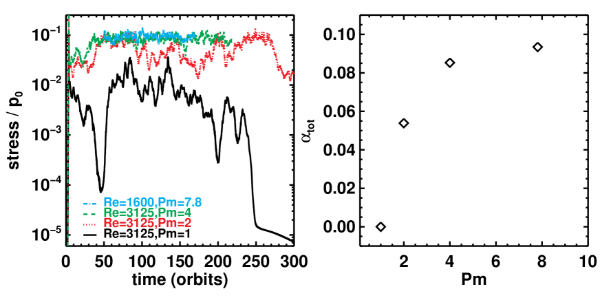
Figure 11: Left: Time evolution of volume averaged total stress for different magnetic Prandtl number $\rm{Pm}$; Right: Time averaged total stress-to-pressure ratio as a function of $\rm{Pm}$. All curves are calculated using resolution $128/H$. We set $\alpha_{\rm tot}=0$ for $\rm{Pm}=1$ case(run x1y4z4r128pm1), as turbulent transport vanishes after $250$ orbits. The saturated stress level is sensitive to the magnetic Prandtl number when $\rm{Pm}\lesssim 4$; however this dependence becomes less significant when $\rm{Pm}\gtrsim 4$, unlike the linear dependence found in standard boxes (Fromang et al., 2007; Simon & Hawley, 2009).

We find for $\rm{Pm}\gtrsim 4$ (run x1y4z4r128pm4 and x1y4z4r128pm8), sustained stress and magnetic energy are achieved in tall boxes. Moreover, the saturated stress and magnetic energy for these runs are not much different from those without explicit dissipation. The time and volume averaged total stress is $\simeq 0.085$ for run x1y4z4r128pm4, and $0.092$ for x1y4z4r128pm8, comparing to $0.084$ for run x1y4z4r128 without explicit dissipation (see Figure 11 and Table 1). We find, in Figure 12, both the volume averaged stresses and magnetic energy spectra are quite similar to the tall box runs without explicit dissipation as shown in right columns of Figure 2 and 3. It would seem that for taller boxes, in which the nonlinear regime and saturation is controlled by dynamo action at least in the $\rm{Pm}\gtrsim 4$ regime, including explicit dissipation has little effect on the results. We note that the saturated stress, $\alpha_{\rm tot}\sim 0.085$ owning to the large scale mean field, t is much greater than the values reported in run SZRe3125Pm4 of Simon & Hawley (2009)($\sim 0.013$), and in run 128Re3125Pm4 of Fromang et al. (2007) ($\sim 0.009$). We also note that the shape of the power spectrum is different than the standard short box simulations with explicit dissipation (Fromang, 2010) as the large scale dynamo observed in our tall box runs is completely absent in this latter case.

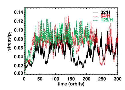
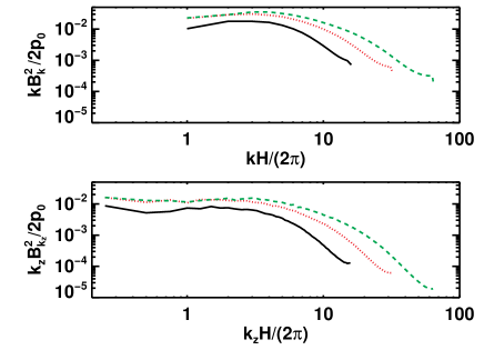
Figure 12: Similar to Figure 2 and 3 but with explicit dissipation:$\rm{Re}=3125$ and $\rm{Rm}=12500$. The results are very similar to the runs without explicit dissipation in Figure 2 and 3.

When $\rm{Pm}=2$ (run x1y4z4r128pm2), the stress in Figure 11 appears to be more bursty compared to higher Prandtl number runs and those without explicit dissipation. The large fluctuations might be a result of competition between super-transient decay and dynamo growth (Thaler & Spruit, 2015). Time averaging over the last $200$ orbits, we find $\alpha_{\rm tot}\sim 0.05$, almost twice smaller than high $\rm{Pm}$ runs. The same parameters have also been explored previously using a standard box, see run 128Re3125Pm2 in Figure 8 of Fromang et al. (2007) and SZRe3125Pm2 in Table 1 of Simon & Hawley (2009), in contrast to our tall box run x1y4z4r128pm2, no sustained MHD turbulence is observed in either of these cases.

The only run in which we find turbulence eventually decays is $\rm{Pm}=1$ (run x1y4z4r128pm1 in Figure 11). After about $250$ orbits, both the Maxwell stress and magnetic energy abruptly drop by several orders of magnitude and the flow becomes laminar. This finding confirms the existence of a critical Prandtl number $\rm{Pm}_{c}$ for a given kinetic Reynolds number even when the box is tall ($L_{\rm{z}}/L_{\rm{x}}>1$ and $L_{\rm{y}}/L_{\rm{x}}=4$). Together with the results of $\rm{Pm}=2$ run, it indicates a smaller critical value, $1\lesssim\rm{Pm}_{c}\lesssim 2$, comparing to $\rm{Pm}_{c}=2$-$4$ found in standard boxes (Fromang et al., 2007; Simon & Hawley, 2009). As we mainly varies the $\rm{Re_{M}}$, we caution the readers that the results might possibly reflect the dependence of saturation amplitude of the MRI on another dimensionless number, the Lundquist number $\rm{Lu}\equiv v_{\rm Az}^{2}/\eta\Omega$ (Sano & Stone, 2002). We find the time averaged $\rm{Lu}\simeq 332$, $105$ and $11$ for run x1y4z4r128pm4, x1y4z4r128pm2 and x1y4z4r128pm1 , getting closer to the critical values reported in previous studies with vertical net flux (Lesur & Longaretti, 2007; Turner et al., 2007; Pessah et al., 2007; Masada & Sano, 2008).

The result of Rempel et al. (2010, see their Figure 5), based on the statistics of MRI turbulence in a standard $(L_{\rm{x}}:L_{\rm{y}}:L_{\rm{z}})=(1:\pi:1)$ box, would predict a characterisic decay time $\sim 10$ shear time units for $\rm{Pm}=1$ and $2$ with the same $\rm{Re}=3125$ as used here. However, we find sustained turbulence that lasts more than several thousand shear time units in our $\rm{Pm}=2$ run; and the active time for our $\rm{Pm}=1$ run is $\sim 200$ orbits, or $2000$ shear time units, much longer than the prediction. Moreover, Fromang et al. (2007) find, when changing $\rm{Re}$ from $12500$ to $25000$, the turbulence lifetime of $\rm{Pm}=1$ increases from $\lesssim 40$ orbits to $\sim 100$ orbits. This would suggest a decaying time even shorter than $40$ orbits for $\rm{Re}=3125$ case, therefore much smaller than our result. Clearly, the aspect ratio of the computational domain may play a big role in determining the dynamical lifetime of MRI turbulence (Riols et al., 2015) in the unstratified, no net flux shearing box.

To sum up, we find the Prandtl number dependence of the turbulent stress in our tall box runs is very different from that found earlier using a standard box (see right panel of Figure 11). When $\rm{Pm}\geq 4$, the saturated stress level is insensitive to the inclusion of explicit dissipation. We find converged turbulent stress for runs with and without explicit dissipation. The saturated stress shows stronger dependence when $\rm{Pm}<4$ as it drops linearly from $\rm{Pm}=4$ to $2$. By choosing a taller box which promotes dynamo action, we find the dynamical lifetime of MHD turbulence is extended, and the critical magnetic Prandtl number is reduced compared to the standard smaller box simulations.

4 MODELING THE DYNAMO

4.1 Dynamo cycle period

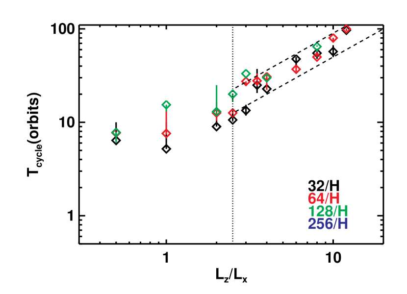
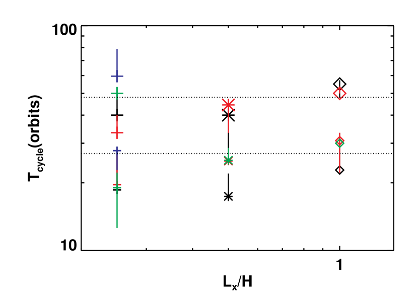
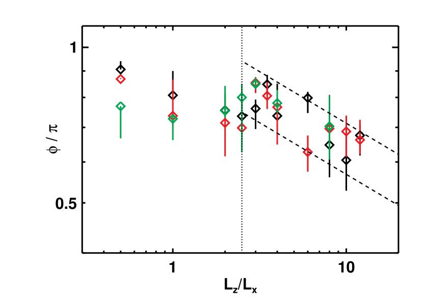
Figure 13: Top: Dynamo cycle periods for different $L_{\rm{z}}/L_{\rm{x}}$ with fixed $L_{\rm{x}}/H=1$, dashed lines show $\propto L_{\rm{z}}/L_{\rm{x}}$ power law. Middle: Dynamo periods vs. box sizes (small symbols for $L_{\rm{z}}/L_{\rm{x}}=4$, and larger symbols for $L_{\rm{z}}/L_{\rm{x}}=8$). The dotted horizontal lines at $T_{\rm{cycle}}=27$ and $48$ orbits show the constancy of cycle period with respect to various box sizes. Bottom: Phase lag between radial and azimuthal mean field as calculated in Equation 13, dashed lines follow $\propto(L_{\rm{z}}/L_{\rm{x}})^{-0.2}$ scaling. The dotted vertical lines at $L_{\rm{z}}/L_{\rm{x}}=2.5$ separate the standard and tall boxes. The error bars of $T_{\rm{cycle}}$ are the variations measured with two independent time sequences; the error bars of phase lag show the max/min values given the variations of the measured $T_{\rm{cycle}}$ and time delay $\Delta t$.

Our previous results indicate that shearing box simulations of the MRI with a large aspect ratio, dynamo action produces strong ordered toroidal fields on vertical scales $L_{\rm{x}}$. In this section we explore models that might explain this dynamo action.

An important property of the dynamo is that at any given vertical location $z$, the toroidal magnetic field is cyclic, and the period of these cycles is an important clue to the mechanism of dynamo action. As illustrated in Figure 4, cyclic patterns of the mean field $\overline{B}_{y}$ becomes strong and regular for those boxes with $L_{\rm{z}}\gtrsim 8\,H$. It is relatively easy to identify the cycle period from the space-time diagrams. However, for smaller boxes, e.g., $L_{\rm{z}}=4\,H$ as shown in Figure 4, the cycle is less regular and it is more difficult to extract a single value of the period $T_{\rm{cycle}}$. Thus, we measure the cycle period based on the power spectrum density (PSD) of the largest vertical mode ($k_{\rm z}=2\pi/L_{\rm{z}}$) of $\overline{B}_{y}(t)$ in Fourier space, i.e.,

$${\rm PSD~{}~{}of~{}~{}}\widetilde{B}_{y}(t),~{}~{}~{}{\rm where~{}~{}~{}}\widetilde{B}_{y}(t)\equiv\int\!\overline{B}_{y}(z;t)e^{-ik_{\rm z}z}dz\,.$$ (12)

We can also estimate errors from the range of $T_{\rm{cycle}}$ as measured from two independent time sequences. We have applied this measurement to all simulations regardless of the box size, but note the physical meaning of $T_{\rm{cycle}}$ in simulations with a small aspect ratio ($L_{\rm{z}}/L_{\rm{x}}<2$) is less clear due to the absence of dynamo action. We list all values of $T_{\rm{cycle}}$ measured in this way in Table 1 for reference.

Once dynamo is at action, there is in general a phase lag between the radial mean field $\overline{B}_{x}$ and the azimuthal $\overline{B}_{y}$. In order to obtain the phase shift, we first apply filter on our mean field and get the largest vertical mode $\overline{\mathbf{B}}^{(1)}(z,t)$, where ‘$(1)$’ denotes $k_{z}=2\pi/L_{\rm{z}}$ only. We then calculate the cross-correlation between two time sequences, $\overline{B}_{x}^{(1)}$ and $\overline{B}_{y}^{(1)}$ at given $z$. The exact time delay $\Delta t$ between radial and azimuthal mean field are the lag which gives the most negative value of correlation. In Table 1, we list the vertically averaged $\Delta t$, and the errors from the variation of $\Delta t$ at different height. The azimuthal mean field therefore lags behind the radial field by

$$\phi=\pi-2\pi\frac{\Delta t}{T_{\rm{cycle}}}$$ (13)

in phase.

In the top panel of Figure 13, we plot the measured $T_{\rm{cycle}}$ for all $L_{\rm{x}}=1\,H$ runs. In general, we find the cycle period is much longer than the dynamical (orbital) time, ranging from several to tens of orbital periods. The measured $T_{\rm{cycle}}$ becomes longer as $L_{\rm{z}}/L_{\rm{x}}$ is increases with a slope slightly shallower than unity. In contrast to the aspect ratio dependence, $T_{\rm{cycle}}$ is not very sensitive to the box size. As shown in the middle panel of Figure 13, $T_{\rm{cycle}}$ for $L_{\rm{z}}/L_{\rm{x}}=4$ scatters between $\sim 20$ and $30$ orbits, while it varies around $\sim 50$ orbits for $L_{\rm{z}}/L_{\rm{x}}=8$ with $\lesssim 50\%$ fluctuations. The phase lag between radial and azimuthal mean field does not depend on box size either (see Table 1). It only weakly depends on the aspect ratio, roughly $\propto(L_{\rm{z}}/L_{\rm{x}})^{-0.2}$ as shown in the bottom panel of Figure 13.

4.2 A toy model

Following the model proposed in Lesur & Ogilvie (2008b), we also try to fit the dynamo cycles observed in our simulations with the following nonlinear model:

$$\partial_{t}\overline{B}^{(1)}_{x}=\gamma\overline{B}^{(1)}_{y}(t-t_{r})\frac{\left|\overline{B}^{(1)}_{y}(t-t_{r})\right|-B_{r}}{B_{r}}\,,$$ (14)

$$\partial_{t}\overline{B}^{(1)}_{y}=-q\Omega\overline{B}^{(1)}_{x}-\beta\overline{B}^{(1)}_{y}(t-t_{r})\,,$$ (15)

where $\overline{B}^{(1)}_{x}$ and $\overline{B}^{(1)}_{y}$ are horizontally averaged radial and azimuthal field that are filtered to conserve only the largest vertical mode ($k_{z}=2\pi/L_{\rm{z}}$, represented with the superscript ‘$(1)$’). Here $t_{r}$ characterizes the time delay between the EMF and large scale magnetic field. When the mean field $|\overline{B}^{(1)}_{y}|$ is smaller than $B_{r}$, the $\gamma$ term effectively amplifies the $\overline{B}^{(1)}_{x}$ field, which in turn lead to $\overline{B}^{(1)}_{y}$ growth via shear. In the opposite case, when $|\overline{B}^{(1)}_{y}|$ exceeds $B_{r}$, the $\gamma$ term starts to damp the radial field, and the azimuthal field is thus reduced via the $\beta$ term. In the fitting, we choose $t_{r}=2/|q\Omega|=4\Omega^{-1}/3$ as suggested by linear analysis (Lesur & Ogilvie, 2008a, b), and $B_{r}/(\sqrt{4\pi\rho_{0}}c_{\rm{s}})=0.3$, a factor $\sim 2.5$ greater than used in (Lesur & Ogilvie, 2008b) to better fit the mean field amplitude observed in our simulations. We then vary $\gamma$ and $\beta$ to match the observed cycle period and long-term amplitude. Empirically, $\gamma$ determines the cycle frequency, and $\beta$ prevent the solution from diverging.

Figure 14: A toy model fit (red, based on Equation 14 and 15) to our unstratified x1y4z8 run (black). The top panel shows the largest vertical mode of mean $\overline{B}_{y}$ at $z=-3\,H$; the bottom panel shows the corresponding radial field. Dotted lines in both panels mark zero amplitude level.

We focus on fitting the results for run x1y4z8r32 as it exhibits a well organized cyclic pattern. Without loss of generality, we fit the filtered $\overline{B}^{(1)}_{x}$ and $\overline{B}^{(1)}_{y}$ at $z=-3\,H$. With $\gamma=2\times 10^{-4}$ and $\beta=4\times 10^{-4}$, the model is shown as the red curves in Figure 14. For times after $100$ orbits, the model provides a reasonable fit to the spatial filtered simulation data. The model predicts the correct dynamo period and relative strength between $\overline{B}^{(1)}_{x}$ and $\overline{B}^{(1)}_{y}$. However the phase shift between $\overline{B}^{(1)}_{x}$ and $\overline{B}^{(1)}_{y}$ is $\pi/2$, slightly smaller than the simulation data, which is $\phi\simeq(0.65\pm 0.08)\pi$. This phase lag is also different than what is found in Herault et al. (2011) ($\sim\pi$), but is close to $3\pi/4$, the phase shift of a marginally excited dynamo wave in a $\alpha$-$\Omega$ dynamo (Brandenburg & Subramanian, 2005). As the values of $B_{r}$ and $t_{r}$ are uncertain, there are likely to be degeneracies in the model parameters.

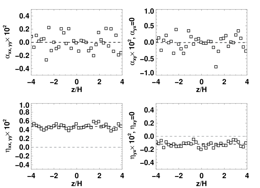
Figure 15: Turbulent transport coefficients measured via simulation at $t=10$-$50$ orbits, assuming closure model like Equation 16. We further set $\alpha_{xx}=\alpha_{yy}$, $\alpha_{yx}=0$, $\eta_{xx}=\eta_{yy}$ and $\eta_{xy}=0$ in this fitting. Square symbols are the time averaged coefficients at evenly spaced disk height. The black dashed lines show the vertical averages and the gray dashed lines are set to zero to help read this plot. Clearly, negative $\eta_{yx}$ is obtained for all $z$ indicating an anti-diffusive growth of magnetic field.

Recent work has explored this model as a magnetic analogue to the ‘shear current’ effect proposed by Rogachevskii & Kleeorin (2004) in which the non-isotropic contribution of the turbulent diffusion can drive large scale magnetic field growth in non-helical turbulent shearing flows. Interestingly, Squire & Bhattacharjee (2015a) recently find negative off-diagonal turbulent diffusivity (a negative $\eta_{yx}$ term which drives exponential growth of $B_{x}$, see their Equation (2) and (3), or Equation 16 in this paper for its definition) by direct measurement in simulations assuming a simple closure model,

$${\mathcal{E}}_{i}=\alpha_{ij}\overline{B}_{j}-\eta_{ij}\epsilon_{jkl}\partial_{k}\overline{B}_{l}\,,~{}~{}~{}~{}i,j,l\in\{x,y\}\,,k=z$$ (16)

where the turbulent EMF, $\mathcal{E}\equiv\overline{v\times b}$, and mean field $\overline{\mathbf{B}}$ can be measured from the simulation data, and $\epsilon_{jkl}$ is the Levi-Civita permutation symbol. After setting $\alpha_{xx}=\alpha_{yy}$, $\alpha_{yx}=0$, $\eta_{xx}=\eta_{yy}$ and $\eta_{xy}=0$, they find an average $\eta_{yx}\sim-10^{-4}H^{2}\Omega$. Following their procedure, i.e. computing $\langle\mathcal{E}_{i}M\rangle$ from Equation 16 for each of $M=(\overline{B}_{x},\overline{B}_{y},\partial_{z}\overline{B}_{x},\partial_{z}\overline{B}_{y})$ and solving the resulting matrix equations at each time point, we also find negative $\eta_{yx}\simeq-1.6\times 10^{-3}H^{2}\Omega$ by time averaging over the dynamo’s growth phase $t=10$-$50$ orbits in x1y4z8r32.

Alternatively, we can also solve Equation 16 at any given $z$ directly assuming time-independent transport coefficients (but a function of height) with multiple linear regression method. The results are shown in Figure 15. All $\alpha$’s fluctuate about zero and are close to zero when averaging over $z$. The diagonal $\eta_{xx}\sim 5\times 10^{-3}H^{2}\Omega$ are dissipations of magnetic field. The non-diagonal term $\eta_{yx}\sim 10^{-3}H^{2}\Omega$ for all $z$ is consistent with that of Squire & Bhattacharjee (2015a), indicates a dynamo growth. We find this negative $\eta_{yx}$ behavior does not change with non-zero $\alpha$’s and $\eta$’s, or unequal $\alpha_{xx}$ and $\alpha_{yy}$, as long as the diagonal $\eta$’s are kept to be the same ($\eta_{xx}=\eta_{yy}$). We also obtain similar values of $\eta_{yx}$ in the well established dynamo cyclic phase using data at $t=100$-$200$ orbits.

However, comparing a time dependent $\eta_{yx}$ throughout a dynamo cycle shows no evidence for sign change when the mean field $|\overline{B}_{y}|$ surpasses some critical magnetic field strength as designed in the toy model, although we do see the filtered EMF $\mathcal{E}_{y}^{(1)}$ changes sign over a cycle with the projection method used in Lesur & Ogilvie (2008b, see their Eqaution (12,13)) and after some smoothing. Further study is still required to explain the inconsistency we find here, and identify the dynamo mechanisms ultimately, but is beyond the scope of this paper.

4.3 Connection to the stratified shearing box

It is interesting to compare the dynamo cycles in our unstratified shearing box simulations with those observed in stratified disks. Simulations using the stratified shearing box always find strong dynamo cycles in the toroidal field (e.g., Brandenburg et al., 1995; Stone et al., 1996; Ziegler & Rüdiger, 2000; Gressel, 2010; Oishi & Mac Low, 2011; Käpylä et al., 2013). As the unstratified shearing box disks approximates the midplane of a stratified disks, there may be some relation between the dynamo behavior seen in both cases.

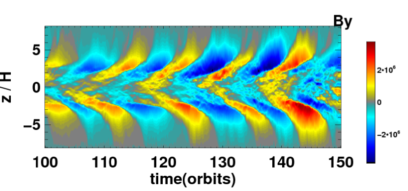
Figure 16: Top: Space-time diagram of $\overline{B}_{y}$ in a stratified box STD32 (Shi et al., 2010). Bottom: a blow-up view of the left to show the main body of the disk within $\pm$ H.

We start by analyzing an existing stratified simulation data (run STD32) first published in Shi et al. (2010). Due to buoyancy, the mean magnetic field is expelled toward the disk surface producing a regular pattern known as the butterfly diagram (see Figure $6$ of Shi et al. (2010)) reproduced here in Figure 16. By extracting data within $\pm H$ of the midplane, we find a clear dynamo cycle with a period $\sim 10$ orbits as shown in the bottom panel of Figure 16. At any given time, the mean azimuthal field is roughly uniform in $z$, and has one sign throughout the subvolume near the midplane (to preserve the constraint of no net flux, field of the opposite sign is located above and below the midplane).

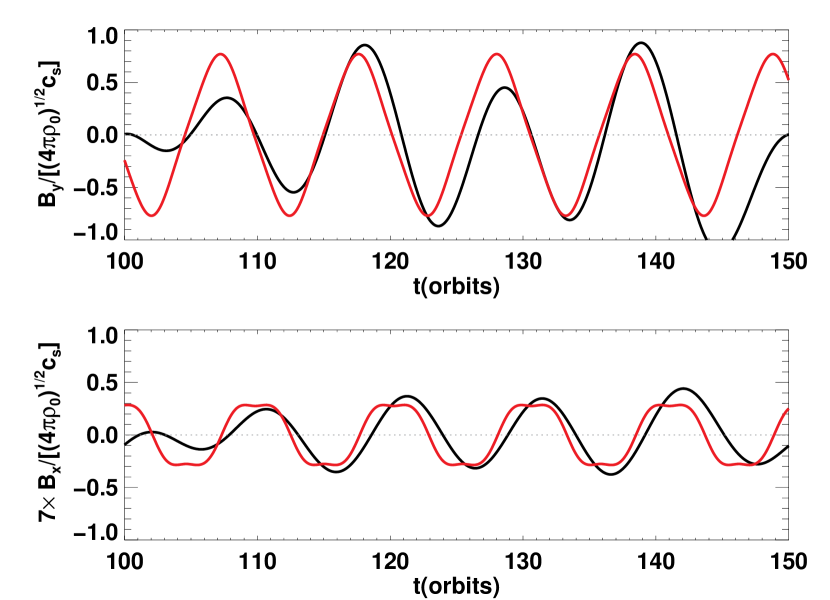
Figure 17: A toy model fit (based on Equation 11 and 12) to the stratified disk STD32 (see Figure 16; Shi et al. (2010)). The fit is in red, the vertically averaged mean $B_{y}$ (top) and $B_{x}$ (bottom) within $\pm$ H are in black. Dotted lines in both panels mark zero amplitude level.

We can also model the dynamo in the stratified shearing box with the toy model described in section 4.2. Again, we adopt $t_{r}=4/(3\Omega)$ and $B_{r}/(\sqrt{4\pi\rho_{0}}c_{\rm{s}})=0.3$, where $\rho_{0}$ and $c_{\rm{s}}$ are the midplane density and sound speed in the stratified disk. We fit the vertically averaged $\overline{B}_{x}$ and $\overline{B}_{y}$ with parameter values of $\gamma=10^{-3}$ and $\beta=0.014$ as shown in Figure 17. Similar to the unstratified case, the toy model captures the cycle period and relative strength of the field components correctly, but slightly underestimates the relative phase between $\overline{B}_{x}$ and $\overline{B}_{y}$ ($\phi/\pi\simeq 0.6^{+0.1}_{-0.2}$).

The overall similarity between the dynamo in the unstratified and stratified disks suggests the same mechanism could act in both cases. We speculate that the core of the stratified disk resembles our tall box runs. Extrapolating the linear scaling found in the left panel of Figure 13 to $L_{\rm{z}}/L_{\rm{x}}\lesssim 2$ gives $T_{\rm{cycle}}\sim 10$ orbits which matches the cycle period of the stratified shearing box very well.

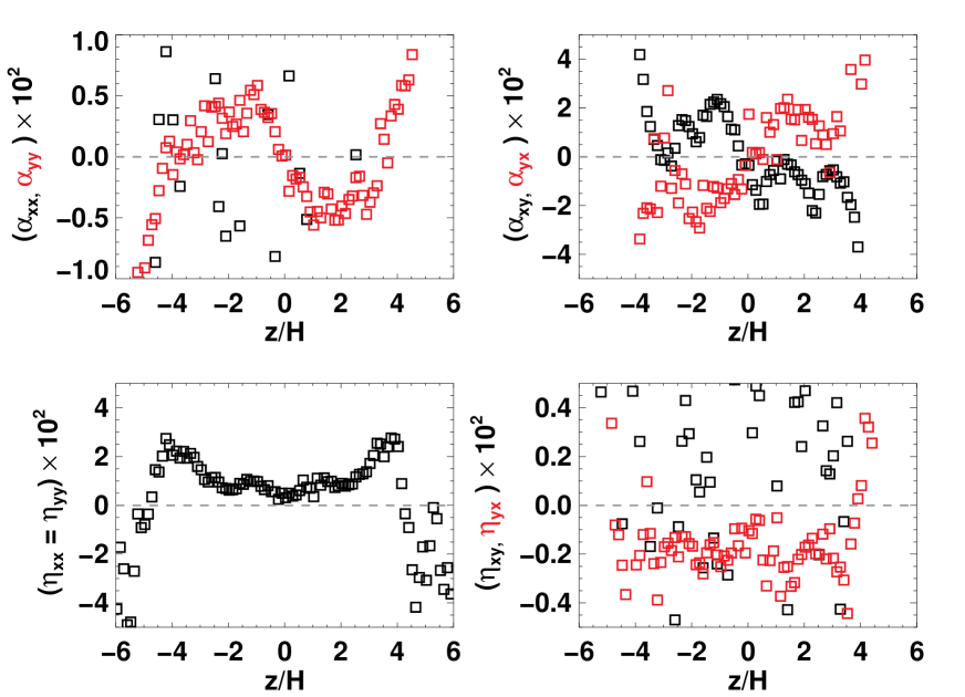
Figure 18: Similar to Figure 15, turbulent transport coefficients measured via stratified disk as in Figure 16 are plotted assuming only $\eta_{xx}=\eta_{yy}$. In each panel, different colors represent different coefficients as labeled on its $y$-axis. We see similar negative $\eta_{yx}$ as in the unstratified disk within $\pm 4\,H$, also a negative (positive) $\alpha_{yy}$ below (above) $4\,H$ in the upper half of the disk, antisymmetric with respect to the midplane.

Assuming similar correlation between EMF and mean field as described in Section 4.2 (Squire & Bhattacharjee, 2015a, b), we find again a negative off-diagonal resistivity $\eta_{yx}\sim-10^{-3}H^{2}\Omega$ (Figure 18), which favors an anti-diffusive dynamo model similar to the unstratified case. However, we find, unlike the unstratified case, an $\alpha$-effect is also present in the stratified box. The diagonal $\alpha_{yy}$ is antisymmetric with respect to the midplane. In the upper half of the disk, it is negative below $4\,H$, and systematically positive above $4\,H$. The negative $\alpha$-effect (within the upper half of the disk) is generally attributed to the dynamo growth in previous stratified simulations and the negative sign is caused by the influence of the field buoyancy and/or strong shear in accretion disks (e.g., Brandenburg et al., 1995; Rüdiger & Pipin, 2000). The positive $\alpha$-effect has also been recently proposed to explain the dynamo (Gressel, 2010; Gressel & Pessah, 2015). Together with the $\eta$-effect, it seems to suggest a combination of direct and indirect dynamo mechanisms (Blackman & Tan, 2004; Gressel, 2010) in stratified shearing box. Further investigations are required to identify whether one or both mechanisms could exist and further cause the dynamo cycles.

5 CONCLUSIONS

In this paper, we have studied MRI turbulence in the unstratified shearing box model with no net flux, and in particular how the size and aspect ratio of the computational domain affects the saturation amplitude and stress. We have performed simulations both with and without explicit dissipation. Previous simulations of this particular shearing box model have shown that the saturation amplitude of the MRI depends on numerical resolution. However, we have shown that the geometry of the computational domain also strongly affects the result. Our main results are summarized as follows:

1. The amplitude of the stress and turbulence driven by the MRI converge to values independent of numerical resolution if the aspect ratio of the computational domain $L_{\rm{z}}/L_{\rm{x}}>2.5$, even without explicit dissipation. These values are proportional to the box size $L_{\rm{x}}^{2}$. Only when the aspect ratio $L_{\rm{z}}/L_{\rm{x}}<2$ do these levels depend on resolution.

2. When $L_{\rm{x}}=H$ and $L_{\rm{z}}/L_{\rm{x}}>2.5$ the converged value of the saturated stress is greatly increased compared to previous values reported for $L_{\rm{z}}/L_{\rm{x}}=1$, and can be as large as $\alpha\gtrsim 0.1$. These values are similar to those required by observations of dwarf novae disks in outburst, perhaps negating some of the concerns expressed in King et al. (2007).

3. The Fourier power spectra of runs with large aspect ratio are very different from those with $L_{\rm{z}}/L_{\rm{x}}\sim 1$. In particular, most of the power in the magnetic field is at small $k$, independent of resolution.

4. For the limited range of parameter values explored in this paper, we find the saturation level of the MRI is independent of whether explicit dissipation (viscosity and resistivity) is included or not, provided that the magnetic Reynolds number is large. Turbulence can be suppressed at small ${\rm Re_{M}}$, corresponding to small magnetic Prandtl number $\rm{Pm}\lesssim 4$, however simulations utilizing a taller box show a relatively smaller critical Prandtl number and much longer lifetime of turbulence than those with $L_{\rm{z}}/L_{\rm{x}}\sim 1$.

5. Cycles of strong large scale toroidal magnetic field with alternating sign on scales of a few $L_{\rm{x}}$ are generated in domains with $L_{\rm{z}}/L_{\rm{x}}>2.5$ via a dynamo. This large scale magnetic field sets and sustains the turbulence independent of numerical resolution.

6. Some aspects of the cyclic dynamo can be modelled with anisotropic turbulent resistivity (Lesur & Ogilvie, 2008b), although the physical mechanisms driving the dynamo are unclear. Similar dynamo cycles observed in a stratified shearing box simulation suggest the stratified and unstratified disks might share common dynamo mechanisms.

As discussed in the Introduction, the unstratified zero-net-flux shearing box model is unlikely to have much relevance to real astrophysical disks. Instead, it is likely that different local ($L\sim H$) patches of the disk are threaded by a broad range of net field strengths, even if the total field threading the disk is zero. Thus, global models of astrophysical disks are best constructed from an ensemble of net flux shearing box simulations. Nevertheless, studies of the unstratified zero-net-flux shearing box are of interest in order to study MHD dynamo action in a simple, well-posed model. Moreover, we have shown that some aspects of the dynamo observed in stratified shearing boxes may be related to properties of the dynamo discussed here. Thus, further study of the MRI dynamo in domains with large aspect ratio, in both compressible and incompressible MHD, and both with and without explicit dissipation are warranted.

References

- Abramowicz et al. (1996) Abramowicz M., Brandenburg A., Lasota J.-P., 1996, MNRAS, 281, L21
- Bai (2014) Bai X.-N., 2014, ApJ, 791, 137
- Bai (2015) Bai X.-N., 2015, ApJ, 798, 84
- Bai & Stone (2011) Bai X.-N., Stone J. M., 2011, ApJ, 736, 144
- Bai & Stone (2013a) Bai X.-N., Stone J. M., 2013a, ApJ, 767, 30
- Bai & Stone (2013b) Bai X.-N., Stone J. M., 2013b, ApJ, 769, 76
- Blackman & Nauman (2015) Blackman E. G., Nauman F., 2015, preprint, (arXiv:1501.00291)
- Blackman & Tan (2004) Blackman E. G., Tan J. C., 2004, Ap&SS, 292, 395
- Blackman et al. (2008) Blackman E. G., Penna R. F., Varnière P., 2008, New Astron., 13, 244
- Bodo et al. (2011) Bodo G., Cattaneo F., Ferrari A., Mignone A., Rossi P., 2011, ApJ, 739, 82
- Bodo et al. (2014) Bodo G., Cattaneo F., Mignone A., Rossi P., 2014, ApJ, 787, L13
- Brandenburg & Subramanian (2005) Brandenburg A., Subramanian K., 2005, Phys. Rep., 417, 1
- Brandenburg et al. (1995) Brandenburg A., Nordlund A., Stein R. F., Torkelsson U., 1995, ApJ, 446, 741
- Davis et al. (2010) Davis S. W., Stone J. M., Pessah M. E., 2010, ApJ, 713, 52
- Fromang (2010) Fromang S., 2010, A&A, 514, L5
- Fromang & Papaloizou (2007) Fromang S., Papaloizou J., 2007, A&A, 476, 1113
- Fromang et al. (2007) Fromang S., Papaloizou J., Lesur G., Heinemann T., 2007, A&A, 476, 1123
- Fromang et al. (2013) Fromang S., Latter H., Lesur G., Ogilvie G. I., 2013, A&A, 552, A71
- Gressel (2010) Gressel O., 2010, MNRAS, 405, 41
- Gressel & Pessah (2015) Gressel O., Pessah M. E., 2015, ApJ, 810, 59
- Gressel & Ziegler (2007) Gressel O., Ziegler U., 2007, Computer Physics Communications, 176, 652
- Guan & Gammie (2011) Guan X., Gammie C. F., 2011, ApJ, 728, 130
- Guan et al. (2009) Guan X., Gammie C. F., Simon J. B., Johnson B. M., 2009, ApJ, 694, 1010
- Hawley & Stone (1998) Hawley J. F., Stone J. M., 1998, ApJ, 501, 758
- Hawley et al. (1995) Hawley J. F., Gammie C. F., Balbus S. A., 1995, ApJ, 440, 742
- Hawley et al. (1996) Hawley J. F., Gammie C. F., Balbus S. A., 1996, ApJ, 464, 690
- Hawley et al. (1999) Hawley J. F., Balbus S. A., Winters W. F., 1999, ApJ, 518, 394
- Hawley et al. (2011) Hawley J. F., Guan X., Krolik J. H., 2011, ApJ, 738, 84
- Heinemann & Papaloizou (2009) Heinemann T., Papaloizou J. C. B., 2009, MNRAS, 397, 64
- Herault et al. (2011) Herault J., Rincon F., Cossu C., Lesur G., Ogilvie G. I., Longaretti P.-Y., 2011, Phys. Rev. E, 84, 036321
- Johnson et al. (2008) Johnson B. M., Guan X., Gammie C. F., 2008, ApJS, 177, 373
- Käpylä et al. (2013) Käpylä P. J., Mantere M. J., Cole E., Warnecke J., Brandenburg A., 2013, ApJ, 778, 41
- King et al. (2007) King A. R., Pringle J. E., Livio M., 2007, MNRAS, 376, 1740
- Kunz & Lesur (2013) Kunz M. W., Lesur G., 2013, MNRAS, 434, 2295
- Lesur & Longaretti (2007) Lesur G., Longaretti P.-Y., 2007, MNRAS, 378, 1471
- Lesur & Ogilvie (2008a) Lesur G., Ogilvie G. I., 2008a, MNRAS, 391, 1437
- Lesur & Ogilvie (2008b) Lesur G., Ogilvie G. I., 2008b, A&A, 488, 451
- Lesur et al. (2013) Lesur G., Ferreira J., Ogilvie G. I., 2013, A&A, 550, A61
- Lesur et al. (2014) Lesur G., Kunz M. W., Fromang S., 2014, A&A, 566, A56
- Masada & Sano (2008) Masada Y., Sano T., 2008, ApJ, 689, 1234
- Masset (2000) Masset F., 2000, A&AS, 141, 165
- Meheut et al. (2015) Meheut H., Fromang S., Lesur G., Joos M., Longaretti P.-Y., 2015, A&A, 579, A117
- Miller & Stone (2000) Miller K. A., Stone J. M., 2000, ApJ, 534, 398
- Oishi & Mac Low (2011) Oishi J. S., Mac Low M.-M., 2011, ApJ, 740, 18
- Pessah et al. (2006) Pessah M. E., Chan C.-K., Psaltis D., 2006, MNRAS, 372, 183
- Pessah et al. (2007) Pessah M. E., Chan C.-k., Psaltis D., 2007, ApJ, 668, L51
- Rempel et al. (2010) Rempel E. L., Lesur G., Proctor M. R. E., 2010, Physical Review Letters, 105, 044501
- Rincon et al. (2007) Rincon F., Ogilvie G. I., Proctor M. R. E., 2007, Physical Review Letters, 98, 254502
- Rincon et al. (2008) Rincon F., Ogilvie G. I., Proctor M. R. E., Cossu C., 2008, Astronomische Nachrichten, 329, 750
- Riols et al. (2013) Riols A., Rincon F., Cossu C., Lesur G., Longaretti P.-Y., Ogilvie G. I., Herault J., 2013, Journal of Fluid Mechanics, 731, 1
- Riols et al. (2015) Riols A., Rincon F., Cossu C., Lesur G., Ogilvie G. I., Longaretti P.-Y., 2015, A&A, 575, A14
- Rogachevskii & Kleeorin (2004) Rogachevskii I., Kleeorin N., 2004, Phys. Rev. E, 70, 046310
- Rüdiger & Pipin (2000) Rüdiger G., Pipin V. V., 2000, A&A, 362, 756
- Salmeron & Wardle (2003) Salmeron R., Wardle M., 2003, MNRAS, 345, 992
- Sano & Stone (2002) Sano T., Stone J. M., 2002, ApJ, 577, 534
- Sano et al. (2004) Sano T., Inutsuka S.-i., Turner N. J., Stone J. M., 2004, ApJ, 605, 321
- Shi et al. (2010) Shi J., Krolik J. H., Hirose S., 2010, ApJ, 708, 1716
- Simon & Hawley (2009) Simon J. B., Hawley J. F., 2009, ApJ, 707, 833
- Simon et al. (2009) Simon J. B., Hawley J. F., Beckwith K., 2009, ApJ, 690, 974
- Simon et al. (2011) Simon J. B., Hawley J. F., Beckwith K., 2011, ApJ, 730, 94
- Simon et al. (2013a) Simon J. B., Bai X.-N., Stone J. M., Armitage P. J., Beckwith K., 2013a, ApJ, 764, 66
- Simon et al. (2013b) Simon J. B., Bai X.-N., Armitage P. J., Stone J. M., Beckwith K., 2013b, ApJ, 775, 73
- Squire & Bhattacharjee (2015b) Squire J., Bhattacharjee A., 2015b, preprint, (arXiv:1508.01566)
- Squire & Bhattacharjee (2015a) Squire J., Bhattacharjee A., 2015a, preprint, (arXiv:1506.04109)
- Stone & Gardiner (2010) Stone J. M., Gardiner T. A., 2010, ApJS, 189, 142
- Stone et al. (1996) Stone J. M., Hawley J. F., Gammie C. F., Balbus S. A., 1996, ApJ, 463, 656
- Stone et al. (2008) Stone J. M., Gardiner T. A., Teuben P., Hawley J. F., Simon J. B., 2008, ApJS, 178, 137
- Suzuki & Inutsuka (2009) Suzuki T. K., Inutsuka S.-i., 2009, ApJ, 691, L49
- Thaler & Spruit (2015) Thaler I., Spruit H. C., 2015, A&A, 578, A54
- Turner et al. (2007) Turner N. J., Sano T., Dziourkevitch N., 2007, ApJ, 659, 729
- Wardle (1999) Wardle M., 1999, MNRAS, 307, 849
- Winters et al. (2003) Winters W. F., Balbus S. A., Hawley J. F., 2003, MNRAS, 340, 519
- Yousef et al. (2008) Yousef T. A., Heinemann T., Schekochihin A. A., Kleeorin N., Rogachevskii I., Iskakov A. B., Cowley S. C., McWilliams J. C., 2008, Physical Review Letters, 100, 184501
- Ziegler & Rüdiger (2000) Ziegler U., Rüdiger G., 2000, A&A, 356, 1141