Symmetries and entanglement in the one-dimensional spin-1/2 XXZ model

Abstract

An efficient and stable algorithm for U(1) symmetric matrix product states (MPS) with periodic boundary conditions (PBC) is proposed. It is applied to a study of correlation and entanglement properties of the eigenstates of the spin-1/2 XXZ model with different spin projections. Convergence properties and accuracy of the algorithm are studied in detail.

I Introduction

Tensor networks and, more specifically, matrix product states (MPS) are convenient ways to represent quantum states. By now, the available literature on this subject is vast, and many different algorithms based on tensor network representations have been proposed and implemented. In particular, the extremely successful DMRG algorithm White (1993) has been rephrased in MPS language Dukelsky et al. (1998), and modern implementations of DMRG use MPS representations. For a detailed review see e.g. Ref. Schollwöck (2011).

The algorithms reviewed in Ref. Schollwöck (2011) use non-symmetric MPS. However, due to the Mermin-Wagner theorem a continuous symmetry cannot be broken Mermin and Wagner (1966) in one dimension (1D). Therefore, for physical as well as numerical reasons it is desirable to construct MPS respecting symmetries, e.g. U(1) or SU(2) symmetry, as dictated by the physical problem under consideration. In fact, SU(2) symmetric MPS have been used already in the early MPS papers by Östlund and Rommer Östlund and Rommer (1995); Rommer and Östlund (1997) in order to optimize the number of MPS parameters to be determined. McCulloch discussed practical issues related to the MPS implementation for Abelian and non-Abelian symmetries McCulloch (2007). More recently, Vidal and collaborators provided a rather systematic presentation of symmetries in tensor networks. In a series of papers Singh et al. (2010, 2011); Singh and Vidal (2012) the essential structure of symmetric tensor network states was clarified.

In the present paper, we propose an efficient and stable algorithm for U(1) symmetric MPS for periodic boundary conditions (PBC). More specifically, we modify the PBC algorithm suggested by Verstraete, Porras, and Cirac Verstraete et al. (2004) and augment it by a novel method to construct U(1) symmetric MPS. Ground or excited states with any desired spin projection can be targeted easily. Theoretical and practical aspects not covered in the more general papers cited above will be addressed and the differences to the more standard open boundary condition (OBC) implementations will be stressed.

We test this algorithm with a rather detailed study of the spin-1/2 XXZ model in an external magnetic field $h$

$$H=\sum_{i=1}^{N}(s_{i}^{x}\otimes s_{i+1}^{x}+s_{i}^{y}\otimes s_{i+1}^{y}+\Delta\,s_{i}^{z}\otimes s_{i+1}^{z})+h\,\sum_{i=1}^{N}s_{i}^{z},$$ (1)

where the index $N+1$ is set to $1$. The spin operators $s_{i}^{\alpha}$ ($\alpha=x,y,z$) are related to the Pauli matrices $\sigma_{i}^{\alpha}$ by $s_{i}^{\alpha}=\sigma_{i}^{\alpha}/2$. The parameters of the model are the anisotropy parameter $\Delta$ and the magnetic field $h$.

This model is U(1) symmetric, i.e. its Hamiltonian $H$ commutes with the $z$-component $S_{z}=\sum_{i=1}^{N}s_{i}^{z}$ of the total spin operator ${\vec{S}}$. Furthermore, it is $Z_{2}$ spin-reflection symmetric. The XXZ model can be solved using the Bethe Ansatz Yang and Yang (1966a, b, c, d); De Pasquale and Facchi (2009); Karbach et al. (1998). These Bethe Ansatz results will serve as a convenient benchmark.

The ground state phase diagram of the spin-1/2 XXZ model as obtained from the Bethe Ansatz is shown in Fig. 1.

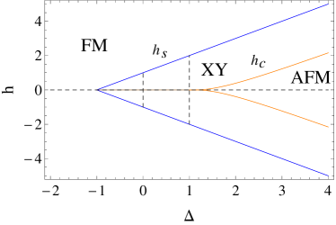
Figure 1: (color online) Phase diagram of the spin-1/2 XXZ model in a magnetic field along $z$ axis. The critical line $h_{s}$ separates the spin liquid (XY) phase from the ferromagnetic (FM) phase. The critical line $h_{c}$ separates the XY phase from the anti-ferromagnetic (AFM) phase. We investigate the model in detail along the dashed lines.

There are three phases: ferromagnetic (FM), spin-liquid (XY), and anti-ferromagnetic (AFM). These three phases are separated by two lines, $h_{s}=1+\Delta$ and $h_{c}$ (see Ref. Yang and Yang (1966d), Eq.(8)). At $h=0$ the XXZ system undergoes a first-order phase transition at $\Delta=-1$ and a Kosterlitz-Thouless infinite-order phase transition at $\Delta=1$ Justino and de Oliveira (2012). The line between these two points is a critical line, where the excitation gap vanishes. This line separates different spin liquid phases. Specifically, we study the model along the lines indicated by dashes in the phase diagram.

The numerical MPS solution provides an explicit representation of the wave functions. Due to the U(1) symmetry the wave functions are simultaneously eigenstates of the Hamiltonian and of $S_{z}$. As a consequence, the magnetization $m_{z}={\langle S_{z}\rangle}/{N}$ can be used as a quantum number to label the states. We determine properties of the XXZ system with different magnetizations $m_{z}$ as a function of the anisotropy parameter $\Delta$. (Alternatively, they could be determined as functions of $\Delta$ and the magnetic field $h$.) It turns out that these states have interesting entanglement properties. In fact, the amount, range, and type of entanglement determines if a state can be successfully modeled by an MPS of a given size. In order to study this quantitatively we will calculate various entanglement quantifiers.

We compare our calculations for 50 and 100 spins with finite-size Bethe Ansatz results. Since spin systems of 100 sites are relatively close to the thermodynamic limit, we also compare with analytical infinite-size Bethe Ansatz results. Furthermore, we discuss convergence problems in detail: convergence to the desired state depends not only on the matrix size $m$ of the MPS but also on the choice of the U(1) symmetry sectors and their degeneracies. Moreover, as our implementation uses the facility introduced in Ref. Pippan et al. (2010) to represent ‘long’ products of large transfer matrices by eventually rather small singular value decompositions, we will study in some detail how this facility can be used profitably in practice. Experience shows that one has to be extremely careful in order not to choose the size of the singular value decomposition too small. In fact, we do not share the positive experience made in Ref. Pippan et al. (2010) for spin-1 Heisenberg systems.

The paper is organized as follows. In section II we outline the PBC MPS formalism used in this paper. Our novel implementation of U(1) symmetric MPS is presented in section III. Application of this algorithm to the 1D spin-1/2 XXZ model together with comparisons to Bethe Ansatz calculations is presented in section IV. Finite size and convergence issues are also discussed there. A few infinite-size Bethe Ansatz results are listed in the Appendix A.

II MPS formalism for PBC

Here we review the PBC formalism proposed by Verstraete, Porras, and Cirac (VPC) Verstraete et al. (2004). We include a number of modifications such as the use of matrix product operators (MPO) and a circular and efficient local update as first suggested by Pippan, White and Evertz (PWE) Pippan et al. (2010). In this and in the next section we denote $s_{i}^{z}$ simply as $s_{i}$ to avoid a large number of indices.

The state of a 1D quantum spin system of size $N$ is approximated in terms of a matrix product state

$$|\psi\rangle=\sum_{\vec{s}}{\rm Tr}\;M^{[1],s_{1}}\cdot\ldots\cdot M^{[N],s_{N}}|s_{1}\dots s_{N}\rangle.$$ (2)

Here, the $s_{i}$ represent the local degrees of freedom at the site $i$, and each $M^{[i],s_{i}}$ represents a matrix of size $m\times m$, where $m$ is called bond dimension, i.e., $M^{[i]}$ is a rank-3 tensor. In the algorithm to be described the elements of these tensors $M_{a_{i-1},a_{i}}^{[i],s_{i}}$ (with $a_{0}=a_{N}$) are variational parameters to be adjusted using a suitable optimization procedure.

Analogously, any operator is written as a matrix product operator

$$O=\sum_{\vec{s},\vec{s}^{\prime}}{\rm Tr}\;W^{[1],s_{1},s_{1}^{\prime}}\ldots W^{[N],s_{N},s_{N}^{\prime}}|s_{1}\dots s_{N}\rangle\langle s_{1}^{\prime}\dots s_{N}^{\prime}|.$$ (3)

Again, each $W^{[i],s_{i},s_{i}^{\prime}}$ represents a matrix of size $m_{W}\times m_{W}$, i.e. each $W^{[i]}$ is a rank-4 tensor with elements $W_{b_{i-1},b_{i}}^{[i],s_{i},s_{i}^{\prime}}$ (with $b_{0}=b_{N}$). In particular, the MPO representation of the XXZ Hamiltonian given in Eq. (1) consists of the following rank-4 tensors,

$$\hat{W}^{[1]} = \begin{pmatrix}hs_{1}^{z}&s_{1}^{x}&s_{1}^{y}&\Delta s_{1}^{z}&\mathds{1}\\ 0&0&0&0&s_{1}^{x}\\ 0&0&0&0&s_{1}^{y}\\ 0&0&0&0&s_{1}^{z}\\ 0&0&0&0&0\end{pmatrix},$$ (4)

$$\hat{W}^{[i]} = \begin{pmatrix}\mathds{1}&0&0&0&0\\ s_{i}^{x}&0&0&0&0\\ s_{i}^{y}&0&0&0&0\\ s_{i}^{z}&0&0&0&0\\ hs_{i}^{z}&s_{i}^{x}&s_{i}^{y}&\Delta s_{i}^{z}&\mathds{1}\end{pmatrix},\hskip 1.42271pti=2,\dots,N.$$ (5)

Matrix elements of an MPO in MPS

$$\langle\phi|O|\psi\rangle={\rm Tr}\;E_{W}^{[1]}(A,B)\cdot\ldots\cdot E_{W}^{[N]}(A,B)$$ (6)

can be conveniently expressed in terms of the (generalized) transfer matrices

$$E_{W}^{[i]}(A,B)=\sum_{s_{i},s_{i}^{\prime}}\,W^{[i],s_{i},s_{i}^{\prime}}\otimes(B^{[i],s_{i}})^{*}\otimes A^{[i],s_{i}^{\prime}}.$$ (7)

The tensors $B$ and $A$ characterize the states $|\phi\rangle$ and $|\psi\rangle$, respectively. The Kronecker product $\otimes$ in Eq. (7) obviously produces matrices of size $m_{W}m^{2}\times m_{W}m^{2}$. The special transfer matrix $E_{1}^{[i]}(A,B)$ represents the matrix element $\langle\phi|\psi\rangle$ of the identity operator.

In order to find the ground state of a many body system one solves a standard variational problem using the matrix elements of the MPS as variational parameters. The optimization of the variational parameters of the MPS is implemented as a local update step, which is repeated until convergence is achieved Verstraete et al. (2004). In the MPO formalism for PBC such a local update step amounts to the solution of a generalized eigenvalue problem

$$H_{\rm eff}^{[i]}\,\nu^{[i]}=\epsilon^{[i]}\,N_{\rm eff}^{[i]}\,\nu^{[i]}$$ (8)

in terms of the effective Hamiltonian $H_{\rm eff}^{[i]}$ and the effective normalization matrix $N_{\rm eff}^{[i]}$ given by

$$H_{\rm eff}^{[i]} = \sum_{k,l=1}^{m_{W}}W^{[i]}_{kl}\otimes\widetilde{\left(({H_{R}^{[i]}\cdot H_{L}^{[i]}})_{lk}\right)},$$ (9)

$$N_{\rm eff}^{[i]} = \mathds{1}\otimes\left(\widetilde{N_{R}^{[i]}\cdot N_{L}^{[i]}}\right).$$ (10)

The matrices $H_{L}^{[i]},~{}N_{L}^{[i]}$ and $H_{R}^{[i]},~{}N_{R}^{[i]}$ are the products of transfer matrices from all sites to the left and to the right of the site $i$, where the MPS is updated. (In order to define which sites are left or right of a site $i$ one initially arbitrarily numbers all sites from 1 to $N$, and sites with $j<i$ are left and sites with $j>i$ are right of site $i$.) The $H$ and $N$ matrices are obtained from transfer operators $E^{[j]}$ as defined in Eq. (7) with the MPO of the Hamiltonian for $H$ and the unity MPO for $N$, in both cases setting $A=B=M^{[j]}$.

The tilde in (9) and (10) indicates the operation $X_{(ij),(kl)}=\tilde{X}_{(ik),(jl)}$ for each $m^{2}\times m^{2}$ matrix. As a consequence of this transposition the effective Hamiltonian and the normalization matrix are assured to be Hermitian matrices and standard methods for the solution of generalized eigenvalue problems can be applied.

The energy of the state is obtained from $\epsilon^{[i]}$, and this value will converge to the ground state energy eventually. In fact, we stop the iterative update procedure, if this quantity does not change any more with respect to defined convergence criteria. The updated MPS is obtained from the generalized eigenvector

$$\nu_{(s_{i},a_{i},a_{i-1})}^{[i]}=M_{a_{i-1},a_{i}}^{[i],s_{i}}$$ (11)

by a suitable partitioning of the vector into a tensor.

The tensors $H_{L}^{[i]},~{}N_{L}^{[i]}$, $H_{R}^{[i]},~{}N_{R}^{[i]}$ can be calculated in different ways. In the VPC approach Verstraete et al. (2004); Schollwöck (2011) one sweeps back and forth over the entire system. The tensors are calculated straightforwardly by successive multiplication by the appropriate transfer matrix $E_{W}^{[i]}$ or $E_{1}^{[i]}$, starting from the leftmost and rightmost sites of the system, respectively. In the PWE approach Pippan et al. (2010); Weyrauch and Rakov (2013); Rossini et al. (2011) one subdivides the system into three sections and optimizes the MPS always from left to right in each section and ‘moves’ (updates) in a circle.

The PWE approach is able to take advantage of the fact that ‘long’ products of transfer matrices have singular values that may decay rather fast. In the PWE approach the minimum length of a product of transfer matrices is $N/3$, so that for a system with size of about 100 spins this length may already be ‘long’. Thus $H_{L}^{[i]},~{}N_{L}^{[i]}$, $H_{R}^{[i]},~{}N_{R}^{[i]}$ may be replaced by their singular value decomposition (SVD) with only a small number of singular values kept, thus dramatically reducing the computational resources required to calculate these tensors. The number of singular values we keep is called $p$ for $N$-tensors and $p^{\prime}$ for $H$-tensors. One finds that $p$ and $p^{\prime}$ depend approximately linearly on the bond dimension $m$ Weyrauch and Rakov (2013); Rossini et al. (2011). Our experience shows that the PWE method has to be used with caution in order to prevent the algorithm from becoming unstable. We will comment on this further in section IV.

Whatever update strategy is used, one runs over the entire system several times updating the MPS at each site until convergence of the energy $\epsilon^{[i]}$ is achieved. Initially, one starts from a randomly selected MPS. After each update step the local MPS tensor is regauged in order to keep the algorithm stable. This means, we have to assure that one of the following relations hold for each local tensor

$$Q^{L} = \sum_{s_{i}}M^{[i],s_{i}{\dagger}}M^{[i],s_{i}}=\mathds{1},\text{left-normalization}$$

$$Q^{R} = \sum_{s_{i}}M^{[i],s_{i}}M^{[i],s_{i}{\dagger}}=\mathds{1},\text{right-normalization}$$ (12)

This is possible because local MPS tensors are only defined up to a gauge freedom.

We would like to mention that it is easily possible to construct excited states along similar lines by finding the lowest state in the space orthogonal to the space spanned by the states already found Porras et al. (2006); Wall and Carr (2012).

III U(1) covariant MPS

In this section we construct U(1) symmetric MPS. First we describe the construction of U(1) invariant MPS (with spin projection $S_{z}=0$) and then covariant MPS with given $S_{z}$. The approach is general and applies to any U(1) symmetric system (i.e., not only to a spin system).

The construction of MPS invariant under a symmetry is described in detail in many papers (see, e.g., Singh et al. (2011)). Each local tensor decomposes into a structural part and a degeneracy part according to the Wigner-Eckart theorem. Thus for U(1) symmetry the bond indices decompose into a spin projection index and a degeneracy index: $a_{i}=\{m_{i},\alpha_{i}\}$; where $\alpha_{i}=1$ through $t_{m_{i}}$ enumerate the degeneracy of a particular $m_{i}$. In practice one has to choose appropriate finite sets $\{m_{i}\}$ with corresponding $\{t_{m_{i}}\}$. They are not determined by symmetry; this fact introduces significant additional freedom into the algorithm.

For U(1) symmetry the Wigner-Eckart theorem takes a very simple form, and the matrix elements are given by

$$M_{(m_{i-1},\alpha_{i-1}),(m_{i},\alpha_{i})}^{[i],s_{i}}=T_{(m_{i-1},\alpha_{i-1}),(m_{i},\alpha_{i})}^{[i]}\cdot\delta_{m_{i-1},m_{i}+s_{i}}.$$ (13)

The matrix elements $T_{(m_{i-1},\alpha_{i-1}),(m_{i},\alpha_{i})}^{[i]}$ of the degeneracy part are often called ‘reduced matrix elements’. In the case of U(1) symmetry the reduced matrix elements are equal to the standard matrix elements, if the latter are nonzero.

Alternatively, it may be said that the local tensors decompose into a block structure, and the positions of the nonzero blocks are determined by the ‘conservation law’

$$m_{i-1}=m_{i}+s_{i},$$ (14)

while the size of the blocks is determined by the degeneracy indices.

The construction (13) of U(1) symmetric matrices encodes the symmetry information within the matrix layout. No separate ‘quantum number’ labels are required. If we want to maintain this property for the construction of the algorithm then for PBC the leftmost and the rightmost indices must be the same, and the procedure described above only constructs U(1) invariant states, i.e. states with $S_{z}=0$. The clue for the practical construction of U(1) covariant MPS for PBC is obtained from Refs. McCulloch (2001, 2007); Singh et al. (2011): a fictitious charge $-S_{z}$ (i.e., a non-interacting spin with spin projection $-S_{z}$) is inserted into the system at an arbitrary position. The modified system has total spin projection $S_{z}=0$ and can be described by a U(1) invariant tensor network.

For convenience, let us insert the fictitious charge at site $N+1$, i.e. between site $N$ and site 1. The tensor at the new site is a single matrix (because $s_{N+1}=-S_{z}$), and its matrix elements are

$$M_{(m_{N},\alpha_{N}),(m_{N+1},\alpha_{N+1})}^{[N+1],-S_{z}}=\\ =T_{(m_{N},\alpha_{N}),(m_{N+1},\alpha_{N+1})}^{[N+1]}\cdot\delta_{m_{N},m_{N+1}-S_{z}}.$$ (15)

The corresponding MPO at this fictitious site is just a unity MPO, since the site should be non-interacting. Using this modified MPS one determines a U(1) invariant state and its corresponding energy as described in the previous section.

In order to find the required U(1) covariant state one eliminates the ‘fictitious charge’ by multiplying its matrix into the tensor of a neighboring site, e.g. each of the matrices $M^{[N],s_{N}}$ is multiplied to matrix $M^{[N+1],-S_{z}}$.

Then, the matrix elements of the new tensor $M^{\prime\,[N]}$

$$\hat{M}_{(m_{N-1},\alpha_{N-1}),(m_{N},\alpha_{N})}^{\prime\,[N],s_{N}}=\\ =T_{(m_{N-1},\alpha_{N-1}),(m_{N},\alpha_{N})}^{\prime\,[N]}\cdot\delta_{m_{N-1},m_{N}+s_{N}-S_{z}}$$ (16)

fulfill the ‘conservation law’

$$m_{N-1}+S_{z}=m_{N}+s_{N}.$$ (17)

It can be easily checked explicitly that the resulting MPS has spin projection $S_{z}$ as required. The conservation law (17) is different from the conservation law (13) fulfilled at the other sites of the system.

The matrix $\hat{M}^{[N+1],-S_{z}}$ is strongly off-diagonal for large $|S_{z}|$. As a consequence, for a given $m$ and $S_{z}$ this matrix may vanish, i.e. cannot be constructed. E.g., to construct a random MPS for $m_{z}=1/2$ for a system of $N$ sites one needs at least $N+1$ degeneracy sectors, which is prohibitive for practical calculations. For smaller $m_{z}$ the minimal number of required degeneracy sectors is smaller, but unlike the $m_{z}=1/2$ state these states are strongly entangled and need enough parameters for a suitable representation. As a consequence, the algorithm may converge to a wrong energy or get unstable: the MPS would be a bad variational Ansatz with too few parameters.

Here, we propose a way for the construction of U(1) covariant MPS for PBC that does not run into such problems. In fact, we propose to insert fictitious charges at several sites within the system. This leads to an MPS with the following matrix elements,

$$M_{(m_{i-1},\alpha_{i-1}),(m_{i},\alpha_{i})}^{[i],s_{i}}=T_{(m_{i-1},\alpha_{i-1}),(m_{i},\alpha_{i})}^{[i]}\delta_{m_{i-1}+x_{i},m_{i}+s_{i}}$$ (18)

with $x_{i}$ fixed at each site and $\sum_{i=1}^{N}x_{i}=S_{z}$. The Kronecker delta in Eq. (18) implies that the $x_{i}$ can only be half-integer or integer.

It can be easily checked by insertion into Eq. (2) that the matrices defined in Eq. (18) produce an MPS with the desired spin projection $S_{z}$. The difference between this approach and the (naive) approach described above is that the total charge $S_{z}$ is distributed among all spins. This can be done because U(1) symmetry is Abelian.

The ‘conservation law’ to be fulfilled at each site

$$m_{i-1}+x_{i}=m_{i}+s_{i}$$ (19)

must be supplemented with the condition $\sum_{i}x_{i}=S_{z}$. For $m_{z}=1/2$ the choice of $x_{i}$ is obvious: $x_{i}=s_{i}=1/2$ at each site, and only one degeneracy sector for the virtual indices is needed. But for $m_{z}<1/2$ these conditions can be fulfilled in various ways. We choose one of them, which distributes $S_{z}$ over all spins as homogeneously as possible. To this end, $S_{z}$ is split into small portions, namely 1/2 for spin-1/2 systems.

Since $|S_{z}|\leq\frac{N}{2}$ for spin-1/2 systems, $x_{i}=0$ for a certain number of sites and $x_{i}=\frac{1}{2}$ for the others. We place all nonzero $x_{i}$ at one end of the system and all zero $x_{i}$ at the other end (with respect to our enumeration $1,\ldots,N$ of the sites). Thus, the conservation laws are

$$m_{i-1} = m_{i}+s_{i}-{\rm Sgn}(S_{z})\cdot\frac{1}{2},~{}~{}~{}{\rm for}~{}i\leq 2|S_{z}|$$ (20)

$$m_{i-1} = m_{i}+s_{i},~{}~{}~{}~{}{\rm for}~{}i>2|S_{z}|.$$ (21)

The MPS matrices are block main/lower/upper diagonal. Let us introduce the following notations: $\textsf{d}\equiv$ block diagonal, $\textsf{ld},\textsf{lld},\dots\equiv$ block 1st, 2nd, …lower diagonal, $\textsf{ud},\textsf{uud},\dots\equiv$ block 1st, 2nd, …upper diagonal. Using this notation let us illustrate how the structure of the matrices look like: for $S_{z}\geq 0$

$$\{\hat{M}^{-1/2},\hat{M}^{1/2}\}=\begin{cases}\{\textsf{uud},\textsf{d}\},&i\leq 2S_{z}\\ \{\textsf{ud},\textsf{ld}\},&i>2S_{z}\end{cases}$$

and for $S_{z}<0$

$$\{\hat{M}^{-1/2},\hat{M}^{1/2}\}=\begin{cases}\{\textsf{d},\textsf{lld}\},&i\leq 2|S_{z}|\\ \{\textsf{ud},\textsf{ld}\},&i>2|S_{z}|.\end{cases}$$

For completeness we also provide results for spin-1. For spin-1 systems $|S_{z}|\leq N$, and we split $S_{z}$ into portions of 1 here. The conservation laws are:

$$m_{i-1} = m_{i}+s_{i}-{\rm Sgn}(S_{z})\cdot 1,~{}~{}{\rm for}~{}~{}i\leq|S_{z}|$$ (22)

$$m_{i-1} = m_{i}+s_{i}~{}~{}~{}~{}{\rm for}~{}~{}~{}i>|S_{z}|,$$ (23)

and the structure of the matrices is for $S_{z}\geq 0$

$$\{\hat{M}^{-1},\hat{M}^{0},\hat{M}^{1}\}=\begin{cases}\{\textsf{uud},\textsf{ud},\textsf{d}\},&i\leq S_{z}\\ \{\textsf{ud},\textsf{d},\textsf{ld}\},&i>S_{z}\end{cases}$$

and for $S_{z}<0$

$$\{\hat{M}^{-1},\hat{M}^{0},\hat{M}^{1}\}=\begin{cases}\{\textsf{d},\textsf{ld},\textsf{lld}\},&i\leq|S_{z}|\\ \{\textsf{ud},\textsf{d},\textsf{ld}\},&i>|S_{z}|.\end{cases}$$

In order to explicitly build up a U(1) symmetric matrix, one has to choose the dimensions of the degeneracy spaces for the bond dimensions. In practice, we have to take a suitable set $D=\{t_{m_{1}},t_{m_{2}},\ldots,t_{m_{n}}\}$, where the $t_{m_{i}}$ denote the dimension of each degeneracy space. For a U(1) symmetric product state the choice would be $D=\{1\}$, and for an entangled state it may be, e.g., $D=\{1,1,3,3,1,1\}$. The set $D$ is not determined by the symmetry and in principle many possibilities exist. There is no a priori principle which dictates a suitable choice.

In practical implementations one just has to ensure the specific block structure of the matrices in order to maintain U(1) symmetry and obtain an MPS with the desired spin projection $S_{z}$. There are many ways to do this in practice, and details depend on the software system used to implement the algorithm. In particular, the obvious sparseness of the matrices must be employed in order to save computational resources. In our implementation we use the sparse matrix technology available in Mathematica 10. This requires very little programming effort. We only have to realize two facts: 1) the matrices $Q^{L,R}$ defined in Eq. (II) are block diagonal for U(1) symmetric MPS, so the regauging can be done blockwise; 2) the generalized eigenvalue problem which must be solved in order to update a local matrix should contain only reduced matrix elements, i.e. rows and columns of zeros in $H_{\rm eff}$ and $N_{\rm eff}$ corresponding to the zeros of the MPS (caused by the block diagonal structure) must be removed before one starts to solve the eigenvalue problem. After each update step we reconstruct the full structure of each local tensor as a sparse tensor. Of course, one could implement the algorithm in terms of reduced tensors only. But the sparse tensor technology employed here saves resources in a similar way and is easier to implement.

IV Application to the spin-1/2 XXZ model

Let us finally apply the algorithm developed above to a physically interesting model, the spin-1/2 XXZ model. Due to the Mermin-Wagner theorem Mermin and Wagner (1966) the continuous U(1) symmetry of the model cannot be broken, while the $Z_{2}$ symmetry is broken in the ferromagnetic and anti-ferromagnetic phases. As a consequence the magnetizations in the $x$ and $y$ axes direction vanish ($m_{x}=m_{y}=0$) as do the corresponding staggered magnetizations ($\bar{m}_{x}=\bar{m}_{y}=0$). Furthermore, for the correlators it holds, that $\langle s_{i}^{x}\otimes s_{i+1}^{y}\rangle=\langle s_{i}^{y}\otimes s_{i+1}^{x}\rangle=0$, and $\langle s_{i}^{x}\otimes s_{i+1}^{x}\rangle=\langle s_{i}^{y}\otimes s_{i+1}^{y}\rangle$. We confirmed that all these relations hold numerically in our calculations.

Furthermore, due to the U(1) symmetry the $z$-magnetization $m_{z}=\langle S_{z}\rangle/N$ is a conserved quantity, which may be used to label the various states of the system. In fact, the ground states in the XY and antiferromagnetic phases have $m_{z}=0$, while in the ferromagnetic phase the ground state has $m_{z}=1/2$. However, in the present paper we will study not only the ground state in the different phases, but also states with different $m_{z}$, e.g. the state with $m_{z}=0$ in the ferromagnetic region, which has interesting entanglement properties. But we will only study the ground state in different $m_{z}$ sectors.

The 2-spin reduced density matrix of the XXZ model may be easily expressed in terms of the spin correlators Syljuåsen (2003), and in view of the U(1) symmetry the density matrix takes the following form

$${\rho_{12}=\begin{pmatrix}\frac{1}{4}+\mathcal{Z}+m_{z}&0&0&0\\ 0&\frac{1}{4}-\mathcal{Z}+\bar{m}_{z}&E-\Delta\mathcal{Z}-hm_{z}&0\\ 0&E-\Delta\mathcal{Z}-hm_{z}&\frac{1}{4}-\mathcal{Z}-\bar{m}_{z}&0\\ 0&0&0&\frac{1}{4}+\mathcal{Z}-m_{z}\end{pmatrix}}.$$ (24)

To bring the density matrix into this form we used that $E=2\langle s_{i}^{x}\otimes s_{i+1}^{x}\rangle+\Delta\,\mathcal{Z}+hm_{z}$ due to Eq. (1). The density matrix $\rho_{12}$ is completely specified in terms of $E$, the magnetization $m_{z}$, the correlator $\mathcal{Z}=\langle s_{i}^{z}\otimes s_{i+1}^{z}\rangle$, and the staggered magnetization $\bar{m}_{z}=\frac{1}{2}\langle s_{i}^{z}-s_{i+1}^{z}\rangle$. Numerically these quantities can be calculated using Eq. (6) and appropriate MPOs for each observable.

The single spin reduced density matrix is obtained as a partial trace of $\rho_{12}$ over the second site,

$$\rho_{1}=\begin{pmatrix}\frac{1}{2}+m_{z}+\bar{m}_{z}&0\\ 0&\frac{1}{2}-m_{z}-\bar{m}_{z}\end{pmatrix}.$$ (25)

From this density matrix one immediately obtains the one-tangle,

$$\tau_{1}=4\det\rho_{1}=1-4(m_{z}+\bar{m}_{z})^{2},$$ (26)

which we will use as an entanglement quantifier of XXZ states. It characterizes the entanglement between one site and the rest of the system.

Other entanglement quantifiers we shall use are the concurrence of formation Wootters (1998) and the concurrence of assistance Laustsen et al. (2003) defined as

$$C_{F}(\rho_{12}) = \max(0,\lambda_{1}-\lambda_{2}-\lambda_{3}-\lambda_{4}),$$ (27)

$$C_{A}(\rho_{12}) = \lambda_{1}+\lambda_{2}+\lambda_{3}+\lambda_{4},$$ (28)

where $\lambda_{1},\lambda_{2},\lambda_{3},\lambda_{4}$ are the square roots of the eigenvalues (in decreasing order) of the non-Hermitian matrix $\rho_{12}\tilde{\rho}_{12}$ with $\tilde{\rho}_{12}=(\sigma_{y}\otimes\sigma_{y})\rho_{12}^{*}(\sigma_{y}\otimes\sigma_{y})$ and $\rho^{*}_{12}$ the complex conjugate of $\rho_{12}$. The concurrence of formation quantifies the nearest-neighbor two-site entanglement, while the concurrence of assistance measures the maximal bipartite entanglement which can be obtained while doing measurements on the rest of the spins.

In the following we will study properties of the spin-1/2 XXZ model as a function of the anisotropy parameter $\Delta$ for various $m_{z}$ using the formulas given above. Numerical calculations are presented for system sizes of $N=50$ and $N=100$ sites. The results are compared to analytical results as well as Bethe Ansatz calculations.

We test if the MPS determined by our algorithm is an eigenstate of the Hamiltonian by calculating the variance per site $\delta H=\sqrt{\langle H^{2}\rangle-\langle H\rangle^{2}}/N$. For an eigenstate it holds that $\delta H=0$. The calculation of $\langle H^{2}\rangle$ is briefly discussed in Appendix B.

IV.1 Correlators and entanglement properties at $h=0$

In the tables 1 and 2 we present results for the XXZ model without magnetic field calculated for periodic systems with $N=50$ spins at different $m_{z}$. For $\Delta=0$ the obtained ground state energies are compared to the analytical result De Pasquale and Facchi (2009)

$$E_{0}(m_{z})=-\frac{1}{N\sin\frac{\pi}{N}}\,\cos(\pi m_{z}),$$ (29)

while for $\Delta=1$ they are compared to finite system Bethe Ansatz calculations Karbach et al. (1998). The one-tangle and the concurrence of assistance indicate that entanglement monotonously grows from the product state $m_{z}=1/2$ to the state $m_{z}=0$, but nearest-neighbor entanglement peaks somewhere off $m_{z}=0$ for $\Delta=1$, thus indicating somewhat complicated entanglement structure. For the entangled states $m_{z}<1/2$ a rather intricate choice of degeneracy set $D$ is required for a reasonable precision of the energy. This issue will be discussed in more detail in the following subsection.

Furthermore, in the tables we list our choice for the numbers $p$ and $p^{\prime}$ of singular values to be kept in the SVD of $N_{L}^{[i]}$, $N_{R}^{[i]}$, $H_{L}^{[i]}$, $H_{R}^{[i]}$. We ensure that the ratio (largest singular value)/(lowest kept singular value) is about $10^{-11}$ as recommended in Pippan et al. (2010). It holds that $p_{\rm max}=m^{2}$ and $p_{\rm max}^{\prime}=2m^{2}$ for the XXZ Hamiltonian (this can be obtained by Gauss elimination of the transfer matrix Weyrauch and Rakov (2013)). We checked that for the spin-1 Heisenberg model the singular values decay very fast for systems of size $N=100$ as observed in Ref. Pippan et al. (2010). On the contrary, for spin-1/2 XXZ model a large percentage of singular values (at least 30%) must be kept for a system of 100 sites. For sizes $N>150$ the parameters $p$, $p^{\prime}$ can be reduced roughly proportionally to ${1}/{N^{2}}$. So $p$ and $p^{\prime}$ must be controlled carefully throughout the algorithm by monitoring the ratio (largest singular value)/(lowest kept singular value).

$m_{z}$	$E$	$E_{T}$	$\Delta E$	$\mathcal{Z}$	$\tau_{1}$	$C_{F}$	$C_{A}$	degeneracy set	$m$	$p~{}p^{\prime}$
0.5	0	0		0.25	0	0	0	$\{1,1,1\}$	3	9 18
0.4	-0.098423	-0.098428	$5.1\cdot 10^{-5}$	0.150316	0.359993	0.165020	0.231194	$\{1\times 4,2,2,3,3,3,2,2,1\times 4\}$	25	625 1250
0.3	-0.187144	-0.187221	$4.1\cdot 10^{-4}$	0.055058	0.640004	0.263648	0.500524	$\{1\times 8,2,3\times 8,2,1\times 8\}$	44	1830 3600
0.2	-0.257447	-0.257688	$9.3\cdot 10^{-4}$	-0.025888	0.840037	0.312642	0.754026	$\{1\times 8,2,3\times 8,2,1\times 8\}$	44	1480 2950
0.1	-0.302792	-0.302930	$4.6\cdot 10^{-4}$	-0.081479	0.960063	0.334296	0.934246	$\{1\times 8,2,3\times 8,2,1\times 8\}$	44	1640 3200
0	-0.318517	-0.318519	$6.3\cdot 10^{-6}$	-0.101456	1.000000	0.339946	1.000000	$\{1\times 3,2,3,4,5,5,5,4,3,2,1\times 3\}$	39	1240 2490

Table 1: The energy $E$, the spin correlator $\mathcal{Z}$ and the entanglement quantifiers $\tau_{1}$, $C_{F}$ and $C_{A}$ as functions of $m_{z}$ for spin-1/2 XXZ model of $50$ sites at $\Delta=0$, $E_{T}$ is calculated according to Eq. (29), $\Delta E=(E-E_{T})/E_{T}$. The staggered magnetization $\bar{m}_{z}$ is zero to a high precision. The dispersion $\delta H$ for $m_{z}=0$ is $3.5\cdot 10^{-4}$.

$m_{z}$	$E$	$E_{T}$	$\Delta E$	$\mathcal{Z}$	$\tau_{1}$	$C_{F}$	$C_{A}$	degeneracy set	$m$	$p~{}p^{\prime}$
0.5	0.25	0.25	0	0.25	0	0	0	$\{1,1,1\}$	3	9,18
0.4	0.051743	0.051741	$3.5\cdot 10^{-5}$	0.150092	0.359998	0.179531	0.216983	$\{1\times 5,2,3\times 6,2,1\times 5\}$	32	1024 2048
0.3	-0.134075	-0.134268	$1.4\cdot 10^{-3}$	0.051847	0.639977	0.305155	0.462994	$\{1\times 8,2,3\times 8,2,1\times 8\}$	44	1640 3200
0.2	-0.291461	-0.292021	$1.9\cdot 10^{-3}$	-0.039533	0.839907	0.372763	0.710159	$\{1\times 8,2,3\times 9,2,1\times 8\}$	47	1680 3335
0.1	-0.401968	-0.402081	$2.9\cdot 10^{-4}$	-0.113493	0.959960	0.391109	0.912827	$\{1\times 8,2,3\times 9,2,1\times 8\}$	47	1870 3690
0	-0.443474	-0.443477	$6.7\cdot 10^{-6}$	-0.147826	1.000000	0.386944	1.000000	$\{1,3,5,7,7,7,5,3,1\}$	39	1190 2360

Table 2: The energy $E$, the spin correlator $\mathcal{Z}$ and the entanglement quantifiers $\tau_{1}$, $C_{F}$ and $C_{A}$ as functions of $m_{z}$ for spin-1/2 XXZ model of $50$ sites at $\Delta=1$, $E_{T}$ is calculated from Bethe Ansatz Karbach et al. (1998), $\Delta E=(E-E_{T})/E_{T}$. The staggered magnetization $\bar{m}_{z}$ is zero to a high precision. The variance $\delta H$ for $m_{z}=0$ is $4.1\cdot 10^{-4}$.

Analogous results for $N=100$ spins for $\Delta=0$ and $\Delta=1$ are presented in Tables 3 and 4, respectively. This system is already large enough that we can also compare to infinite system Bethe Ansatz energies. For convenience, we briefly review the necessary formulas in the Appendix A. Infinite system Bethe Ansatz results are available analytically and the whole phase diagram sketched in Fig. 1 is easily obtained. Finite size Bethe Ansatz results are not available to us for the whole range of $\Delta$.

$m_{z}$	$E$	$E_{T}$	$E_{\infty}$	$\Delta E$	$\mathcal{Z}$	$\tau_{1}$	$C_{F}$	$C_{A}$	degeneracy set	$m$	$p~{}p^{\prime}$
0.5	0	0	0		0.25	0	0	0	$\{1,1,1\}$	3	9 18
0.4	-0.097939	-0.098379	-0.098363	$4.5\cdot 10^{-3}$	0.150	0.360	0.158	0.237	$\{1\times 4,2,2,3\times 3,2,2,1\times 4\}$	25	290  580
0.3	-0.183044	-0.187129	-0.187098	$2.2\cdot 10^{-2}$	0.058	0.640	0.229	0.522	$\{1\times 8,2,3\times 8,2,1\times 8\}$	44	590 1150
0.2	-0.245605	-0.257560	-0.257518	$4.6\cdot 10^{-2}$	-0.016	0.839	0.248	0.775	$\{1\times 8,2,3\times 8,2,1\times 8\}$	44	970 1720
0.1	-0.296970	-0.302780	-0.302731	$1.9\cdot 10^{-2}$	-0.076	0.960	0.310	0.937	$\{1\times 8,2,3\times 8,2,1\times 8\}$	44	1120 2050
0	-0.318340	-0.318362	-0.318310	$6.9\cdot 10^{-5}$	-0.101	1.0	0.339	1.0	$\{1,1,1,2,3,4,5\times 3,4,3,2,1,1,1\}$	39	835 1650

Table 3: The energy $E$, the spin correlator $\mathcal{Z}$ and the entanglement quantifiers $\tau_{1}$, $C_{F}$ and $C_{A}$ as functions of $m_{z}$ for spin-1/2 XXZ model of $100$ sites at $\Delta=0$, $E_{T}$ is calculated according to Eq. (29), $\Delta E=(E-E_{T})/E_{T}$. The staggered magnetization $\bar{m}_{z}$ is zero to a high precision. The variance $\delta H$ for $m_{z}=0$ is $5.2\cdot 10^{-4}$.

$m_{z}$	$E$	$E_{T}$	$E_{\infty}$	$\Delta E$	$\mathcal{Z}$	$\tau_{1}$	$C_{F}$	$C_{A}$	degeneracy set	$m$	$p~{}p^{\prime}$
0.5	0.25	0.25	0.25	0	0.25	0	0	0	$\{1,1,1\}$	3	9 18
0	-0.443205	-0.443230	-0.443147	$5.7\cdot 10^{-5}$	-0.148	1.0	0.386	1.0	$\{1,3,5,7\times 3,5,3,1\}$	39	725 1450

Table 4: The energy $E$, the spin correlator $\mathcal{Z}$ and the entanglement quantifiers $\tau_{1}$, $C_{F}$ and $C_{A}$ as functions of $m_{z}$ for spin-1/2 XXZ model of $100$ sites at $\Delta=1$, $E_{T}$ is calculated from Bethe Ansatz Karbach et al. (1998), $\Delta E=(E-E_{T})/E_{T}$. The staggered magnetization $\bar{m}_{z}$ is zero to a high precision. The variance $\delta H$ for $m_{z}=0$ is $6.6\cdot 10^{-4}$.

In Fig. 2 we compare the infinite size Bethe Ansatz energies with numerical results for $N=100$ in the parameter interval $-2<\Delta<4$. The ground state energy at $m_{z}=0$ for $\Delta\geq-1$ agrees with Bethe Ansatz results up to finite-size corrections $\Delta E/E\sim 10^{-4}$. For $\Delta\leq-1$ and infinite system size the ground state energies $E_{0}(m_{z})={\Delta}/{4}$ are independent of $m_{z}$ Yang and Yang (1966a), which means that in this parameter region the ground state is infinitely degenerate. The degeneracy of the states with different $m_{z}$ is obtained numerically at $\Delta=-1$ with high precision.

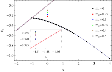
Figure 2: (color online) Energy per site $E(m_{z})$ for a spin-1/2 XXZ ring of 100 sites at zero magnetic field as a function of the anisotropy parameter $\Delta$. The full line shows the Bethe Ansatz result Eq. (Appendix A: Infinite size Bethe Ansatz results). The various symbols described in the legend correspond to numerical results for selected $m_{z}$. The inset shows results at $\Delta=-1.5$ for $m_{z}=.5$, .49, .48, .47, .46, .45.

However, for finite systems the degeneracy is lifted for $\Delta<-1$ (Fig. 2 inset). The energy per site of the state with $m_{z}=1/2-1/N$ is given by an exact solution

$$~{}E_{0}=\Delta/4+(|\Delta|-1)/N$$ (30)

indicating a quite significant finite site effect at rather moderate $\Delta$. The corresponding numerical result shown in Fig. 2 (inset) exactly agrees with Eq. (30). In addition, in the inset of Fig. 2 we show results for a few other states with large magnetization which show even larger finite size effects.

In Fig. 3 the staggered magnetization $\bar{m}_{z}$ is displayed for a system with $N=100$ compared to the Bethe Ansatz result given in the Appendix A. As expected, one finds that the staggered magnetization is non-zero only in the anti-ferromagnetic region $\Delta>1$. For $1\leq\Delta\lesssim 1.4$ we observe large finite-size effects. In addition, we show in Fig. 3 results for the one-tangle calculated from $\bar{m}_{z}$ using Eq. (26). The result indicates that the $m_{z}=0$ state is strongly entangled for $\Delta<1$. Above $\Delta=1$ this state slowly ‘looses’ entanglement with increasing $\Delta$. In order to obtain correct numerical results for the staggered magnetization at $-1<\Delta<1$ it is important that U(1) symmetry is preserved. Typically non-symmetric codes obtain spurious results for $\bar{m}_{x}$ (which becomes nonzero) and consequently for $\tau_{1}$.

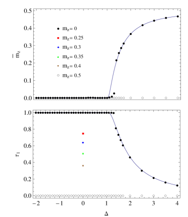
Figure 3: (color online) Staggered magnetization per site $\bar{m}_{z}$ (top) and one-tangle $\tau_{1}$ (bottom) of the 1D spin-1/2 XXZ ring of 100 sites at zero magnetic field as a function of the anisotropy parameter $\Delta$. Numerical results (symbols) are compared to results calculated from Eqs. (Appendix A: Infinite size Bethe Ansatz results) and (26). Significant finite-size effects are observed for $1\leq\Delta\lesssim 1.4$.

Finally, we present results for the concurrence of formation $C_{F}$ and the concurrence of assistance $C_{A}$ for a system of 100 sites in Fig. 4 again compared to infinite size Bethe Ansatz results. One observes for $C_{A}$ large finite size effects close to the critical point at $\Delta=1$. The trace for the concurrence of assistance $C_{A}$ looks very similar to that of $\tau_{1}$. However, the concurrence of formation $C_{F}$ shows a very different characteristic as it is maximal at $\Delta=1$ and zero for $\Delta<-1$. In this respect the $m_{z}=0$ XXZ state for $\Delta<-1$ is similar to the Greenberger-Horne-Zeilinger (GHZ) state, which has zero concurrence of formation but is highly entangled with one-tangle or concurrence of assistance equal to 1.

There is a somewhat indirect quantification of entanglement: the bond size $m$ of the matrices of the MPS as given in the tables. The required bond sizes $m$ for states with large but not full magnetization indicate that these states are characterized by entanglement not measured by the simple quantifiers $\tau_{1}$, $C_{F}$, or $C_{A}$. Long-ranged entanglement or many-way entanglement may be a better way to quantify the entanglement of these states.

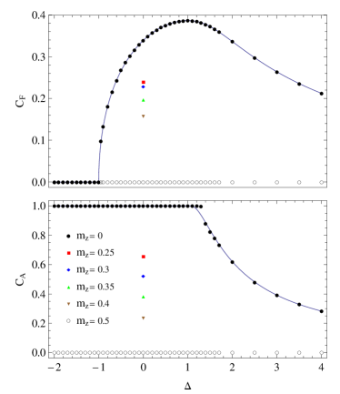
Figure 4: (color online) (top) Concurrence of formation $C_{F}$ of 1D spin-1/2 XXZ ring of 100 sites at zero magnetic field as a function of the anisotropy parameter $\Delta$ compared to Bethe Ansatz results (full line). (bottom) Concurrence of assistance $C_{A}$ of 1D spin-1/2 XXZ ring of 100 sites at zero magnetic field as a function of the anisotropy parameter $\Delta$ compared to Bethe Ansatz results (full line). Significant finite-size effects are observed for $1\leq\Delta\lesssim 1.4$.

IV.2 Accuracy and precision of the algorithm

The results presented in the previous section are meant to illustrate the algorithm, and we did not attempt to push the calculations to the limit in order to obtain the best possible accuracy. Nevertheless, with relatively small MPS sizes one obtains results in quite good agreement with other approaches.

As is obvious from the results, the accuracy depends crucially on the chosen degeneracy set, which also determines the overall MPS size $m$. Of course, since the algorithm is variational, it entails an iterative minimization, and the number of iteration steps taken is another important parameter. Often we can easily increase the precision of our results by adopting more stringent convergence requirements at the expense of a longer computing time. For the present paper we stopped our numerical update (i.e. minimization) procedure if the averaged relative ground state energy does not change more than $10^{-7}$ within the last $N/3$ update steps of the algorithm. However, it is possible that for a given degeneracy set $D$ the approach to the minimum may be excessively slow, and the optimization stops before reaching the minimum. Moreover, occasionally the algorithm may get stuck in a local minimum.

It would be desirable that the algorithm chooses an optimal degeneracy set $D$ automatically. For OBC such a procedure exists, and we will briefly review this method here. It was introduced by White White (2005) and entails a modification of the regauging step. Instead of Eqs. (II) the following constructions are calculated,

$$\rho_{(a_{i-1},s_{i}),(a_{i-1}^{\prime},s_{i}^{\prime})}=\sum_{a_{i}}M^{[i],s_{i}}_{a_{i-1},a_{i}}M^{[i],s_{i}^{\prime}*}_{a_{i-1}^{\prime},a_{i}}~{}~{}\text{left-n.},$$

$$\rho_{(s_{i},a_{i}),(s_{i}^{\prime},a_{i}^{\prime})}=\sum_{a_{i-1}}M^{[i],s_{i}}_{a_{i-1},a_{i}}M^{[i],s_{i}^{\prime}*}_{a_{i-1},a_{i}^{\prime}}~{}~{}\text{right-n.},~{}~{}~{}$$ (31)

$\rho$ has size $(2s+1)m\times(2s+1)m$. Its SVD $\rho=USV^{{\dagger}}$ has exactly $m$ singular values, and therefore $\rho$ has matrix rank $m$, and one obtains the regauged matrix $M^{[i],s_{i}}_{a_{i-1},a_{i}}=U_{(a_{i-1},s_{i}),a_{i}}$. This matrix is identical to the one obtained from Eqs. (II). It can be shown that for OBC the constructions (IV.2) corresponds to the reduced density matrix $\rho_{1\rightarrow i}$ for the sites from 1 to $i$ (left-normalization) and $\rho_{i\rightarrow N}$ for the sites from $i$ to $N$ (right-normalization), respectively. They can be calculated here from a single tensor $M^{[i]}$.

In the case of U(1) symmetry $\rho$ is block diagonal with each block corresponding to a quantum number $m_{i-1}-s_{i}$ (left-normalization) or $s_{i}+m_{i}$ (right-normalization). Due to the ‘conservation laws’ each nonzero block of $\rho$ corresponds to an analogous block of $Q^{L,R}$, and corresponding blocks have the same rank. Thus regauging can be done block-wise, and the same results are obtained as if Eqs. (II) were used.

The crucial step proposed by White White (2005) for OBC is a modification of the density matrix $\rho$ (see, e.g. Eq. (217) in Ref. Schollwöck (2011)). The matrix rank of the modified density matrix is larger than $m$. Again one calculates an SVD of this matrix $\rho=USV^{{\dagger}}$ and constructs the regauged local tensor $M^{[i]}$ from the matrix $\tilde{U}$ corresponding to the $m$ largest singular values. For U(1) symmetric MPS one selects the $m$ largest singular values irrespective to which degeneracy sector they belong. In this way degeneracy sectors may increase or decrease in size or sectors may even be lost or created dynamically during the optimization procedure.

Unfortunately, this procedure does not work for PBC: The reduced density matrix $(\rho_{1\rightarrow i})$ (needed for left-normalization) is for both OBC and PBC given by

$$(\rho_{1\rightarrow i})_{(s_{1},\cdots,s_{i}),(s_{1}^{\prime},\cdots,s_{i}^{\prime})}=\\ {\rm Tr}((M^{[1],s_{1}}\otimes M^{[1],s_{1}^{\prime*}})\cdots(M^{[i],s_{i}}\otimes M^{[i],s_{i}^{\prime*}})\cdot N_{R}^{*}),$$ (32)

and in general it involves all MPS tensors. However, for OBC $N_{R}=1$ and, as alluded to above, the rank of $\rho$ is only $m$, and $\rho$ can be written in terms of a single tensor $M^{[i]}$. This simplification does not happen for PBC, and the reduced density matrix has size and rank $d^{i}$.

From these considerations we see that the construction of an algorithm for the selection of degeneracy sets for PBC faces different issues than for OBC, and we here opted to determine them by numerical tests as was also done by Vidal and collaborators Singh and Vidal (2012) for U(1) symmetric MERA implementations. As a consequence, an alternative to the approach proposed in White (2005) for OBC is desirable, but beyond the scope of the present paper.

V Conclusion

In this paper we propose a specific new way to construct U(1) covariant MPS for PBC and discuss many aspects concerning the construction of symmetric MPS not covered elsewhere. We implement our proposal in a variational algorithm for finite spin systems based on the PBC algorithm of Verstaete, Porras, and Cirac Verstraete et al. (2004) as modified by Pippan, White, and Evertz Pippan et al. (2010).

The algorithm is applied to a study of the properties of the spin-1/2 XXZ model for systems of 50 and 100 sites. It proves to be numerically stable, and our results agree rather well with predictions of the Bethe Ansatz. The algorithm correctly captures the properties of the system in the XY phase, where other numerical algorithms break the U(1) symmetry.

The convergence properties of the proposed algorithm are studied. Our concrete choice of appropriate U(1) degeneracy sectors is provided, and we exemplify that the replacement of long products of transfer matrices by their truncated singular value decomposition (SVD) must be used with caution. We demonstrate, that one must keep many more singular values than for spin-1 systems discussed in Ref. Pippan et al. (2010).

We calculate various spin correlation functions and entanglement quantifiers for the XXZ model as a function of the anisotropy parameter $\Delta$ and the magnetization $m_{z}$ at zero magnetic field. We show analytically and numerically that entanglement in general decreases monotonically with increasing magnetization of the system. The concurrence of formation shows a deviation from this rule for systems with small magnetization.

The present work could be extended in many ways. Most importantly a general algorithmic strategy to choose the appropriate degeneracy sectors is needed. In this way it may be also possible to improve the numerical results for intermediate spin projections $m_{z}$. Such work is presently under way as a generalization of the proposal made by White White (2005) for OBC.

Appendix A: Infinite size Bethe Ansatz results

The energy per site of the $m_{z}=0$ state as determined by the infinite size Bethe Ansatz Yang and Yang (1966a, c) is given by

$$E_{0} = \frac{\Delta}{4}~{}~{}~{}~{}~{}~{}~{}~{}~{}~{}~{}~{}~{}~{}~{}~{}~{}~{}~{}~{}~{}~{}~{}~{}~{}~{}~{}~{}~{}~{}~{}~{}{\rm for}~{}~{}\Delta\leq-1,$$ (33)

$$E_{0} = \frac{\Delta}{4}-\frac{1}{2}(1-\Delta^{2})\times~{}~{}~{}~{}~{}~{}~{}~{}~{}~{}~{}{\rm for}~{}~{}\Delta>-1$$

$$~{}~{}\int\limits_{-\infty}^{\infty}\frac{dx}{\cosh\pi x(\cosh(2x\arccos\Delta)-\Delta)}.$$

At $\Delta=1$ the integrand is not well defined, and one needs to take an appropriate limit. One obtains the $\mathcal{Z}$ correlator from a derivative of the energy with respect to $\Delta$.

The staggered magnetization $\bar{m}_{z}$ is given by Baxter (1973),

$$\bar{m}_{z}=0~{}~{}~{}{\rm if}~{}\Delta<1,$$

$$\bar{m}_{z}=\frac{1}{2}\prod_{n=1}^{\infty}\tanh^{2}(n~{}{\rm arccosh}\,\Delta)~{}~{}~{}~{}{\rm if}~{}\Delta\geq 1.$$ (35)

From these results the complete density matrix Eq. (24) can be determined, which enables the calculation of the entanglement quantifiers discussed in section IV.

Appendix B: Calculation of $\langle H^{2}\rangle$

The MPO for the calculation of $\langle H^{2}\rangle$ is given by

$$\mathcal{W}_{(b_{i-1}b_{i-1}^{\prime}),(b_{i}b_{i}^{\prime})}^{[i],s_{i},s_{i}^{\prime}}=\sum_{s_{i}^{\prime\prime}}W_{b_{i-1},b_{i}}^{[i],s_{i},s_{i}^{\prime\prime}}\,W_{b_{i-1}^{\prime},b_{i}^{\prime}}^{[i],s_{i}^{\prime\prime},s_{i}^{\prime}}.$$

This MPO represents a matrix of size $25\times 25$ for the XXZ model (its explicit form is not written down due to its large size); $\langle H^{2}\rangle$ can be obtained from this MPO using Eq. (6) and appropriate transfer matrices $E_{\mathcal{W}}^{[i]}$ of size $25m^{2}\times 25m^{2}$.

However, it can be shown explicitly by Gauss elimination that all the transfer matrices (and consequently their products) have only $p^{\prime\prime}=6m^{2}$ nonzero singular values. So the multiplication of $N$ transfer matrices can be done by the efficient update proposed in Pippan et al. (2010); Weyrauch and Rakov (2013).