Inter-Vehicle Range Estimation from
Periodic Broadcasts

Abstract

Dedicated short-range communication (DSRC) enables vehicular communication using periodic broadcast messages. We propose to use these periodic broadcasts to perform inter-vehicle ranging. Motivated by this scenario, we study the general problem of precise range estimation between pairs of moving vehicles using periodic broadcasts. Each vehicle has its own independent and unsynchronized clock, which can exhibit significant drift between consecutive periodic broadcast transmissions. As a consequence, both the clock offsets and drifts need to be taken into account in addition to the vehicle motion to accurately estimate the vehicle ranges. We develop a range estimation algorithm using local polynomial smoothing of the vehicle motion. The proposed algorithm can be applied to networks with arbitrary number of vehicles and requires no additional message exchanges apart from the periodic broadcasts. We validate our algorithm on experimental data and show that the performance of the proposed approach is close to that obtained using unicast round-trip time ranging. In particular, we are able to achieve sub-meter ranging accuracies in vehicular scenarios. Our scheme requires additional timestamp information to be transmitted as part of the broadcast messages, and we develop a novel timestamp compression algorithm to minimize the resulting overhead.

I Introduction

I-A Motivation

Intelligent transportation systems have gained significant importance in the recent past with various initiatives taken both by the federal and state transportation agencies in collaboration with the automotive industry. Two major applications in this context are vehicular safety and autonomous driving. A key requirement for both these applications is precise, sub-meter vehicle localization [2] typically enabled through ranging (i.e., distance estimation). Existing technologies such as LiDAR [3] or RTK-GPS [4] that provide such precise ranging have the drawback of being costly to deploy. There is hence a need for precise ranging solutions that are in addition cost effective and commercially viable. As a possible solution to this problem, we explore in this work the use of affordable WiFi hardware for obtaining precise range estimates between vehicles.

The underlying concept of ranging using radio-frequency signals exploits that the propagation delay of the wireless signal from the transmitter to the receiver is proportional to their distance. Time-of-arrival (ToA) ranging [5] typically assumes that the transmitter and receiver are time synchronized in order to calculate the propagation delay. Time-difference-of-arrival (TDoA) ranging [4] uses a small number of time-synchronized reference nodes allowing the other nodes in the system to obtain ranging measurements from these reference nodes without themselves being time synchronized. Finally, round-trip-time (RTT) ranging [6] eliminates the need for time synchronization by exchanges two messages between the transmitter and receiver, from which the common clock offset can be canceled. These two messages need to be exchanged within a short time interval, since otherwise clock drifts can introduce significant ranging errors.

Time synchronization is hard to achieve in vehicular applications particularly when the synchronization accuracy needs to be in the order of nanoseconds to achieve sub-meter level accuracy. This precludes the use of ToA based ranging schemes. Similarly, it may not be practical to establish synchronized reference nodes, which are needed for TDoA based schemes. RTT could be used to obtain relative range estimates between the vehicles. However, a unicast mechanism like RTT requires a significant number of message exchanges especially when the number of vehicles in the network is large. In particular, the number of messages scales quadratically with the number of vehicles.

I-B Summary of Results

In this work, we develop a broadcast mechanism for range estimation that can drastically reduce the number of required message exchanges. In particular, in our proposed scheme, the number of messages being broadcast scales only linearly with the number of vehicles. The broadcast mechanism is motivated by the dedicated short-range communications (DSRC) standard [7], which is a modification of the WiFi standard. The DSRC standard prescribes periodic broadcasting of safety messages by every vehicle. We propose to use these broadcasted safety messages to perform ranging without the need for any additional messaging. Our scheme does require additional information to be transmitted in each DSRC packet, and we introduce a compression mechanism to minimize this overhead.

The contributions of this paper are summarized as follows:

• We develop an algorithm and protocol for range estimation between vehicles based on broadcast message exchanges wherein each vehicle periodically broadcasts a packet with certain timing information. Using this periodic broadcast ranging approach, the number of required message exchanges scales only linearly with the number of vehicles as opposed to quadratically when using standard unicast RTT ranging.

• The time interval between broadcast transmissions can be on the order of $100$ ms. As a consequence, we need to explicitly account for the relative clock offset and clock drift between the vehicles. Further we also need to account for the motion of the vehicles during this time interval.

• We also propose a novel compression algorithm to efficiently quantize and transmit timestamp information in the broadcast packets in order to reduce the protocol overhead. This is particularly significant in the context of DSRC, in which packets have constrained payload size.

• We conduct experiments using Qualcomm-proprietary WiFi hardware that supports ranging capabilities. We show that sub-meter level accuracies are achievable with the proposed algorithm. Finally, the proposed algorithm suffers only a small loss in ranging performance as compared to RTT-based ranging. Thus, the reduction from quadratic number of messages in RTT to linear number of messages in our proposed periodic broadcast ranging algorithm results in only a small loss in ranging performance.

I-C Related Work

Range estimation has been a topic of research interest for several decades starting with classical RADAR systems [8] and GPS [4] to more recent technologies like WiFi [6], Bluetooth [9], and ultra-wide band [10] to name a few. There is still active research in the community to develop inexpensive and precise ranging technologies that can work in various environments. These are enabling applications in the vehicular space [11, 12, 13, 14], sensor networks [15, 16, 17], and robotics [18, 19].

GPS works on the TDoA principle wherein the satellites are time synchronized. RADAR based systems typically work on the principle of electromagnetic reflection. The transmitted signal is reflected off a target object and the received reflected signal can be correlated with the transmitted signal to locate the target. Some high-end cars have RADAR-like sensors that detect distances to obstacles and other vehicles. However, when multiple vehicles are present in the environment it is hard to distinguish between different reflectors. Further, if all the vehicles transmit RADAR pulses without a synchronization protocol, then the resulting interference between the signals can degrade the ranging accuracy.

RTT-based systems are popular and well studied in various contexts. The IEEE 802.11mc task group defines a Fine-Timing-Measurement (FTM) protocol [6] for RTT ranging in the WiFi signal spectrum. As described before, this eliminates the need for clock synchronization, but is inherently unicast in nature. There are quite a few works in the literature that consider the problem of range and location estimation in the presence of unknown clock offsets [20, 21, 22]. Most of these are in the context of location estimation, wherein the location of a node or a set of nodes needs to be estimated from ranging measurements. These works explore the joint estimation of locations and clock offsets. The problem of joint estimation of clock parameters and distances between pairs of mobile nodes is considered in [23], which makes use of the local smoothness of the node trajectories to solve for the unknown variables.

II System Model

We consider a collection of moving vehicles, each equipped with a radio transmitter and receiver, that emit periodic broadcast messages with approximate period of $T$ seconds. Our goal is to estimate the distances between the vehicles using time of departure and arrival information from these broadcast messages. This scenario is motivated by the DSRC standard, in which vehicles broadcast so-called basic safety messages with an approximate period of $T=0.1$ s. We will use DSRC as a running example throughout this paper, however the results apply more generally.

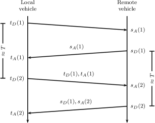
Figure 1: Message exchanges for ranging using periodic broadcasts.

For ease of presentation, we restrict ourselves for now to a scenario with two vehicles, a local and a remote vehicle. The generalization to arbitrary number of vehicles is discussed in Section III-C. We assume that the vehicle clocks are not synchronized. Since the message departure and arrival times are measured with respect to each vehicle’s own clock, we need to explicitly account for the relation between the two clocks. Formally, we denote by $t_{D}(n)$ and $s_{D}(n)$ the departure times of the $n$th message sent by the local and remote vehicle, respectively. Similarly, we denote by $t_{A}(n)$ and $s_{A}(n)$ the arrival times of these messages. These arrival and departure times are piggybacked on the broadcast messages as illustrated in Fig. 1.

We assume that the local time $t$ and the remote time $s$ are related via the linear relationship

$$s(t)=\theta+(1+\delta)t,$$ (1)

where $\theta$ is the clock offset (measured in seconds) and $\delta$ is the clock drift (a unitless quantity). Typical values of $\delta$ are on the order of $\pm 10^{-5}$, which is usually expressed as a drift of $10$ parts per million (ppm); see also Fig. 2.

Figure 2: Experimentally measured WiFi receiver clock drift $\delta$ as a function of time. The experiment is carried out in a static setting, and the parameter $\delta$ is estimated by differencing consecutive measurements.

In the periodic broadcast ranging approach analyzed in this paper, the delay between a message departure and the following message arrival is on the order of $T/2$. Hence, the clock drift during this period is on the order of $\delta T/2$. For example, in the DSRC case with $T=0.1$ s, the drift of a $10$ ppm clock during that time is on the order of $0.5$ $\mu$s. When left uncompensated, this clock drift of $0.5$ $\mu$s will result in a ranging error of approximately $150$ m!

Careful modeling and dealing with clock drifts is hence critical for successful ranging using the periodic broadcast approach. Continuing with the DSRC example, assume we aim for a ranging accuracy on the order of $0.3$ m, then we can tolerate an uncompensated clock drift of at most $0.01$ ppm between successive samples. Fig. 2 suggests that we can therefore model the clock drift as being approximately constant for a window of a few seconds (corresponding to a few tens of DSRC message exchanges). During this time, the model (1) with constant $\delta$ is valid.

The departure and arrival timestamps can then be related as follows:

$$s_{A}(n) =\theta+(1+\delta)t_{D}(n)+d_{D}(n)/c+z_{A}(n),$$ (2a)

$$s_{D}(n) =\theta+(1+\delta)t_{A}(n)-d_{A}(n)/c+z_{D}(n),$$ (2b)

where $d_{D}(n)$ and $d_{A}(n)$ are the inter-vehicle distances at times $t_{D}(n)$ and $t_{A}(n)$, where $c$ is the speed of light, and where $z_{A}(n)$ and $z_{D}(n)$ are additive receiver noise terms assumed to be i... with mean zero and variance $\sigma^{2}$. The timestamp relation (2) assumes that the vehicle movement and the clock drift are negligible during the packet time of flight between the two vehicles. Since this time of flight is less than $300$ ns for vehicle distances less than $100$ m, this assumption is reasonable.

Figure 3: Measured sample vehicle movement and corresponding distances to a fixed receiver (indicated by the large solid dot) as a function of time.

The relation (2) links the departure and arrival timestamps to the inter-vehicle distances $d_{D}(n)$ and $d_{A}(n)$. Because of the movement of the vehicles, these distances are time-varying (i.e., change as a function of $n$). A typical vehicle trajectory and the corresponding distances of the vehicle to the fixed receiver are shown in Fig. 3. Since the vehicle distances can change by several tens of meters per second, this time-varying nature of the distances needs again to be taken into account when using periodic packet broadcasts for ranging. For example, in DSRC with $T=0.1$ s, the change in distances can be on the order of several meters between successive message arrivals.

Recall from Fig. 1 that at time $t_{A}(n)$ of the arrival of message $n$ at the local vehicle, this vehicle has access to all its own measured timestamps $t_{D}(i)$ and $t_{A}(i)$ with $i\leq n$. From the received messages, it has also access to the remotely measured timestamps $s_{A}(i)$ with $i\leq n$ and $s_{D}(i)$ with $i<n$ (note that, due to hardware limitations, $s_{D}(n)$ is not available at the local vehicle at time $t_{A}(n)$). Using this information, our goal in the remainder of this paper is to estimate at time $t_{A}(n)$ the distance $d_{A}(n)$ between the vehicles at that time instant.

Remark 1 (Comparison with RTT Ranging):

One standard approach to measure distances between unsynchronized communication devices is to use unicast RTT based ranging. In this approach, a first communication device sends a unicast ranging request to a second communication device. The second communication device responds with a unicast acknowledgment. By measuring this round-trip time, the first device can then estimate the distance between the two devices.

In the formalism of this paper, RTT ranging computes the distance estimate

$$\hat{d}_{A}(n) =\tfrac{c}{2}\bigl{(}(t_{A}(n)-t_{D}(n))-(s_{D}(n)-s_{A}(n))\bigr{)}$$ (3)

$$=\tfrac{1}{2}(d_{A}(n)+d_{D}(n))+\tfrac{c}{2}\bigl{(}\delta(t_{D}(n)-t_{A}(n))+z_{A}(n)-z_{D}(n)\bigr{)}.$$

In typical RTT applications, the time $t_{A}(n)-t_{D}(n)$ between transmitting the ranging request and receiving the corresponding acknowledgment is small. For example, in the RTT-based WiFi fine-timing measurement protocol, the delay between these two events is on the order of $0.01$ ms. Assuming a $\delta$ of $10$ ppm, the clock drift during that time is on the order of $0.1$ ns, resulting in a ranging error of approximately $1.5$ cm, which is negligible for most applications. Put differently,

$$\tfrac{c}{2}\bigl{(}\delta(t_{D}(n)-t_{A}(n))\approx 0.$$

At the same time, the vehicular movement during those $0.01$ ms is at most $0.1$ cm, so that the change in distances over this period can be ignored as well. Put differently,

$$\tfrac{1}{2}(d_{A}(n)+d_{D}(n))\approx d_{A}(n).$$

Hence, for unicast RTT ranging,

$$\tfrac{c}{2}\bigl{(}(t_{A}(n)-t_{D}(n))-(s_{D}(n)-s_{A}(n))\bigr{)}\approx d_{A}(n)+\tfrac{c}{2}\bigl{(}z_{A}(n)-z_{D}(n)\bigr{)}$$

is an accurate estimate of the vehicular distances at time $t_{A}(n)$, and both drift and vehicular movement can be completely ignored.

As already alluded to earlier, the situation changes completely for periodic broadcast ranging considered in this paper, where $T$ can be quite large. In the DSRC example, $T=0.1$ s. As a result the clock drift error term

$$\tfrac{c}{2}\bigl{(}\delta(t_{D}(n)-t_{A}(n))$$

can be on the order of $150$ m, and the vehicular movement error term

$$d_{A}(n)-\tfrac{1}{2}(d_{A}(n)+d_{D}(n))=\tfrac{1}{2}(d_{A}(n)-d_{D}(n))$$

can be on the order of several meters. Hence, the simple RTT range estimator (3) fails in the periodic broadcast setting, and more sophisticated estimators, explicitly taking into account clock drift and vehicular movement, are needed. We present such an estimator in the next section.

III Ranging Algorithm

We now describe an algorithm for ranging based on periodic broadcasts. The main estimation algorithm is presented in Section III-A. Section III-B proposes a compression scheme for the remote timestamps. How these algorithms can be extended to handle arbitrary number of vehicles is discussed in Section III-C.

III-A Distance Estimation

Recall from (1) that the local time $t$ and the remote time $s$ are related through a clock offset $\theta$ and a clock drift $\delta$. The clock offset can be handled in a straightforward way by defining the timestamp differences

$$\Delta t_{D}(n) \mathrel{\triangleq}t_{D}(n)-t_{D}(n-1),$$

$$\Delta s_{A}(n) \mathrel{\triangleq}s_{A}(n)-s_{A}(n-1),$$

$$\Delta t_{A}(n) \mathrel{\triangleq}t_{D}(n)-t_{A}(n-1),$$

$$\Delta s_{D}(n) \mathrel{\triangleq}s_{A}(n)-s_{D}(n-1).$$

Observe that these quantities were chosen such that $\Delta t_{D}(n)$, $\Delta s_{A}(n)$, $\Delta t_{A}(n)$, and $\Delta s_{D}(n)$ are all available at the local vehicle at time $t_{A}(n)$ (see Fig. 1 in Section II).

The timestamp relation (2) can then be rewritten as

$$\Delta s_{A}(n) =(1+\delta)\Delta t_{D}(n)+(d_{D}(n)-d_{D}(n-1))/c+\Delta z_{A}(n),$$ (4a)

$$\Delta s_{D}(n) =(1+\delta)\Delta t_{A}(n)+(d_{D}(n)+d_{A}(n-1))/c+\Delta z_{D}(n),$$ (4b)

with

$$\Delta z_{A}(n) \mathrel{\triangleq}z_{A}(n)-z_{A}(n-1),$$ (5a)

$$\Delta z_{D}(n) \mathrel{\triangleq}z_{A}(n)-z_{D}(n-1).$$ (5b)

Thus, the transformed measurements are invariant with respect to the clock offset $\theta$. One could further transform the measurements to achieve invariance with respect to the clock drift $\delta$ as well (see Section III-B). However, this would lead to significant noise amplification, and we instead opt to explicitly estimate the nuisance parameter $\delta$.

As was pointed out in Section II, the clock drift $\delta$ can be assumed to be constant during a window of a few seconds. From Fig. 3 in Section II, we see that during the same timescale the inter-vehicular distances vary smoothly. Similar to [23], we make a polynomial approximation of the variation of these inter-vehicle distances as a function of time. Due to the sharp peaks occurring when two vehicles pass each other, we choose the degree of this local polynomial approximation to be two. Formally, we are thus making the approximation

$$d_{A}(n)\approx a_{0}+a_{1}t_{A}(n)+a_{2}t_{A}^{2}(n),$$ (6a)

$$d_{D}(n)\approx a_{0}+a_{1}t_{D}(n)+a_{2}t_{D}^{2}(n).$$ (6b)

Fix a window size $w$, and assume both the clock drift and the distance approximations are valid over $w$ time periods. From (4) and (6), the polynomial coefficients $a_{0}$, $a_{1}$, $a_{2}$, and the nuisance parameter $\delta$ can then be estimated via least-squares as the minimizer $(\hat{\delta},\hat{a}_{0},\hat{a}_{1},\hat{a}_{2})$ of

$$\bigl{(}c\Delta s_{A}(n)-(1+\delta)c\Delta t_{D}(n)-a_{1}t_{D}(n)-a_{2}t_{D}^{2}(n)+a_{1}t_{D}(n-1)+a_{2}t_{D}^{2}(n-1)\bigr{)}^{2}$$

$$\quad{}+\bigl{(}c\Delta s_{D}(n)-(1+\delta)c\Delta t_{A}(n)-2a_{0}-a_{1}t_{D}(n)-a_{2}t_{D}^{2}(n)-a_{1}t_{A}(n-1)-a_{2}t_{A}^{2}(n-1)\bigr{)}^{2}$$

$$\quad{}+\dots$$

$$\quad{}+\bigl{(}c\Delta s_{A}(n-w+1)-(1+\delta)c\Delta t_{D}(n-w+1)-\dots\bigr{)}^{2}$$

$$\quad{}+\bigl{(}c\Delta s_{D}(n-w+1)-(1+\delta)c\Delta t_{A}(n-w+1)-\dots\bigr{)}^{2}$$

This equation can be rewritten in matrix form as

$$\min_{\bm{x}}\,\lVert{\bm{\beta}-\bm{B}\bm{x}}\rVert^{2},$$

with

$$\bm{\beta} \mathrel{\triangleq}c\cdot\begin{pmatrix}\Delta\bm{s}_{A}(n-w+1:n)-\Delta\bm{t}_{D}(n-w+1:n)\\ \Delta\bm{s}_{D}(n-w+1:n)-\Delta\bm{t}_{A}(n-w+1:n)\end{pmatrix}$$

$$\bm{B} \mathrel{\triangleq}\begin{pmatrix}c\Delta\bm{t}_{D}(n-w+1:n)&\!\bm{0}&\!\bm{t}_{D}(n-w+1:n)-\bm{t}_{D}(n-w:n-1)&\!\bm{t}_{D}^{2}(n-w+1:n)-\bm{t}_{D}^{2}(n-w:n-1)\\ c\Delta\bm{t}_{A}(n-w+1:n)&\!\bm{2}&\!\bm{t}_{D}(n-w+1:n)+\bm{t}_{A}(n-w:n-1)&\!\bm{t}_{D}^{2}(n-w+1:n)+\bm{t}_{A}^{2}(n-w:n-1)\end{pmatrix}$$

$$\bm{x} \mathrel{\triangleq}\begin{pmatrix}\delta&a_{0}&a_{1}&a_{2}\end{pmatrix}^{\mathsf{T}}$$

and where we have used the notation

$$\bm{t}^{2}(n-w+1:n)\mathrel{\triangleq}\begin{pmatrix}t^{2}(n-w+1)&t^{2}(n-w+2)&\dots&t^{2}(n)\end{pmatrix}^{\mathsf{T}}.$$

The minimizer of this least-squares problem is

$$\hat{\bm{x}}=(\bm{B}^{\mathsf{T}}\bm{B})^{-1}\bm{B}^{\mathsf{T}}\bm{\beta},$$

from which we can recover the desired distance estimate

$$\hat{d}_{A}(n)=\hat{a}_{0}+\hat{a}_{1}t_{A}(n)+\hat{a}_{2}t_{A}^{2}(n).$$ (7)

As we will see next, this estimate can be improved upon by taking the correlated nature of the transformed ranging noise into account.

Recall from (5) that the transformed noise $\Delta z_{A}(n)$ and $\Delta z_{D}(n)$ is no longer white. In fact, setting

$$\bm{z}_{A} \mathrel{\triangleq}z_{A}(n-w:n)$$

$$\bm{z}_{D} \mathrel{\triangleq}z_{D}(n-w:n)$$

and

$$\Delta\bm{z}_{A} \mathrel{\triangleq}\Delta z_{A}(n-w+1:n)$$

$$\Delta\bm{z}_{D} \mathrel{\triangleq}\Delta z_{D}(n-w+1:n),$$

we can write

$$\begin{pmatrix}\Delta\bm{z}_{A}\\ \Delta\bm{z}_{D}\end{pmatrix}=\bm{J}\begin{pmatrix}\bm{z}_{A}\\ \bm{z}_{D}\end{pmatrix}$$

with

$$\bm{J}\mathrel{\triangleq}\begin{pmatrix}(\bm{0}\ \bm{I})-(\bm{I}\ \bm{0})&\bm{0}\\ (\bm{0}\ \bm{I})&-(\bm{I}\ \bm{0})\end{pmatrix}.$$

Hence,

$$\mathbb{E}\bigl{(}(\Delta\bm{z}_{A};\ \Delta\bm{z}_{D})(\Delta\bm{z}_{A}^{\mathsf{T}}\ \Delta\bm{z}_{D}^{\mathsf{T}})\bigr{)}=\sigma^{2}\bm{J}\bm{J}^{\mathsf{T}}\mathrel{\triangleq}\bm{\Sigma}.$$

Thus, $\bm{\Sigma}^{-1/2}(\bm{\beta}-\bm{B}\bm{x})$ whitens the transformed ranging noise. The corresponding whitened least-squares problem is

$$\min_{\bm{x}}\,\lVert{\bm{\Sigma}^{-1/2}\bm{\beta}-\bm{\Sigma}^{-1/2}\bm{B}\bm{x}}\rVert^{2},$$ (8)

with solution

$$\hat{\bm{x}}=(\bm{B}^{\mathsf{T}}\bm{\Sigma}^{-1}\bm{B})^{-1}\bm{B}^{\mathsf{T}}\bm{\Sigma}^{-1}\bm{\beta}.$$

The estimate $\hat{d}_{A}(n)$ can be recovered from this as before (see (7)).

The computation of $\hat{d}_{A}(n)$ is performed at the local vehicle at each time step $n$ to estimate the distance $d_{A}(n)$ from the remote vehicle at the current time $t_{A}(n)$. We point out that all measurements required to perform the computation of the estimate $\hat{d}_{A}(n)$ are available at the local vehicle at time $t_{A}(n)$.

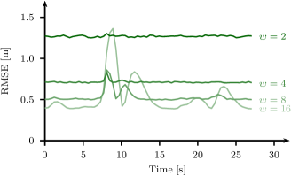
Figure 4: Impact of window size on estimation error. The bottom figure plots the expected root mean-squared error (RMSE) (estimated using $10^{4}$ Monte-Carlo simulations) as a function of time for several fixed window sizes. The top figure shows the corresponding actual distances.

Since we are estimating four parameters, and since there are two measurements at each time step, the window size $w$ needs to be at least two for the matrix $\bm{B}^{\mathsf{T}}\bm{\Sigma}^{-1}\bm{B}$ to be invertible. Larger values of $w$ result in larger noise suppression. On the other hand, too large a value of $w$ will lead to biased estimates due to model mismatch (see Fig. 4). For the setting considered in this paper, a window size of $w=8$ is a reasonable choice.

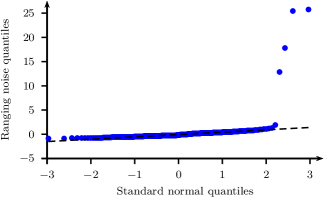
Figure 5: Q-Q plot of ranging noise. The figure shows that the ranging noise exhibits heavy right tail caused by non-line-of-sight measurements.

By performing experiments with known vehicle distances, the ranging noise terms $z_{D}(n)$ and $z_{A}(n)$ can be directly measured. Fig. 5 shows the Q-Q plot for the ranging noise, comparing the empirical ranging noise quantiles to the quantiles of a standard normal distribution. For Gaussian ranging noise, the points in the Q-Q plot should be linearly related.

Fig. 5 indicates that the ranging noise is well modeled by a Gaussian random variable except for the right tail, where the ranging noise exhibits significant outliers. These outliers are caused by non-line-of-sight (NLOS) range measurements, in which the direct path between the transmitter and the receiver is obstructed, and the signal is instead observed via a longer path containing reflections. Dealing with these large NLOS outliers is hence critical, as will be discussed next.

Local polynomial regression can be made more robust to such NLOS outliers by carrying out the least-squares procedure several times and reducing the weight of those observations with large residuals [24]. Formally, denote by

$$\bm{e}\mathrel{\triangleq}\bm{\Sigma}^{-1/2}\bm{\beta}-\bm{\Sigma}^{-1/2}\bm{B}\hat{\bm{x}}$$

the vector of residuals in (8). Compute the median $m$ of $\lvert{\bm{e}}\rvert$ and the robustness weights

$$\gamma_{i}\mathrel{\triangleq}\bigl{(}1-e_{i}^{2}/(36s^{2})\bigr{)}^{2}.$$

Then recompute a weighted least-squares solution with weights $\gamma_{i}$. This procedure is repeated a few times. For our setting, five repetitions yielded good performance.

III-B Timestamp Compression

Recall from Fig. 1 in Section II that the departure and arrival timestamps $s_{D}(n)$ and $s_{A}(n)$ are transmitted from the remote to the local vehicle and similarly for the timestamps $t_{D}(n)$ and $t_{A}(n)$ from the local to the remote vehicle. While for ranging between two vehicles the number of bits that need to be transmitted is manageable, this may no longer be the case when distances need to be estimated frequently and between many vehicles.

As an example, consider again the vehicular DSRC standard (which is a variant of WiFi as mentioned before). The periodic broadcast messages are called basic safety messages (BSM) in the DSRC standard. Each such BSM has a size of $142$ Bytes (in the simplest form) [25]. Now, consider a scenario with $20$ cars within radio range of each other, whose relative distances we aim to estimate. A scenario of this size could easily arise in a multi-lane highway setting, for example. Each vehicle then needs to piggyback $20$ timestamps on each of its broadcast messages (one time of departure from its previously broadcast message, and $19$ times of arrival of the broadcast messages of the other cars, see also the discussion in Section III-C). The FTM protocol of the WiFi standard allocates $48$ bits to the transmission of each of these arrival and departure timestamps quantized to a resolution of $0.1$ ns [6]. This results in a total of $120$ Bytes of data that need to be piggybacked on the broadcast message. Thus, the timestamp overhead to enable the ranging is comparable to the size of the original BSM packet itself.

In this section, we discuss a method to compress the measured timestamps to reduce the overhead of communicating them. The proposed method achieves this compression by making use of prior positional information. Specifically, by using previously received and measured timestamps and by assuming that the vehicles are moving at some bounded speed.

The compression of the timestamps is performed by discarding their most-significant bits. The intuition is that since each vehicle is getting periodic ranging and position estimates from the neighboring vehicle, an approximate distance estimate at the current time is known. This approximate distance information allows to reconstruct the most-significant timestamp bits. It is only the lower-order bits that are needed to enhance the estimation accuracy, and which consequently need to be transmitted.

Formally, denote by $[\Delta s_{A}(n)]$ the compressed timestamp corresponding to $\Delta s_{A}(n)$. Then

$$[\Delta s_{A}(n)]\mathrel{\triangleq}10^{10}\cdot\Delta s_{A}(n)\bmod 2^{L},$$

for some fixed positive integer $L$ to be specified later. Assuming that $\Delta s_{A}(n)$ is measured in integer multiples of $0.1$ nanoseconds, then the quantity $[\Delta s_{A}(n)]$ can be encoded using $L$ bits. These $L$ bits are then transmitted from the remote to the local vehicle.

To recover $\Delta s_{A}(n)$ from $[\Delta s_{A}(n)]$, observe that

$$10^{10}\cdot\Delta s_{A}(n)=[\Delta s_{A}(n)]+k_{A}(n)2^{L}$$

for some integer $k_{A}(n)$. Thus, the aim of the local vehicle is to find $k_{A}(n)$. To this end, we make use of the fact that, by (4),

$$\frac{\Delta s_{A}(n)}{\Delta t_{D}(n)}=1+\delta+\frac{d_{D}(n)-d_{D}(n-1)}{c\Delta t_{D}(n)}+\frac{\Delta z_{A}(n)}{\Delta t_{D}(n)}$$ (9)

so that

$$\frac{\Delta s_{A}(n)}{\Delta t_{D}(n)} -\frac{\Delta s_{A}(n-1)}{\Delta t_{D}(n-1)}$$

$$=\frac{d_{D}(n)-d_{D}(n-1)}{c\Delta t_{D}(n)}-\frac{d_{D}(n-1)-d_{D}(n-2)}{c\Delta t_{D}(n-1)}+\frac{\Delta z_{A}(n)}{\Delta t_{D}(n)}-\frac{\Delta z_{A}(n-1)}{\Delta t_{D}(n-1)}$$

$$\approx\frac{d_{D}(n)-2d_{D}(n-1)+d_{D}(n-2)}{cT}+\frac{\Delta z_{A}(n)-\Delta z_{A}(n-1)}{T},$$

where the approximation is that $\Delta t_{D}(n)\approx\Delta t_{D}(n-1)\approx T$, i.e., that the intervals between broadcast transmissions are approximately constant. If the relative speed of vehicle movement is bounded, and having probabilistic bounds on the behavior of the ranging noise, this implies that

$$\bigg{\lvert}\frac{\Delta s_{A}(n)}{\Delta t_{D}(n)}-\frac{\Delta s_{A}(n-1)}{\Delta t_{D}(n-1)}\bigg{\rvert}\leq\rho$$ (10)

with high probability for some positive constant $\rho$. For a concrete example, in the DSRC context, $T=0.1$ s and we can assume a relative vehicle speed of at most $100$ m/s. Further, assume a ranging noise $\Delta z_{A}(n)$ of less then $10\text{ m}/c$, corresponding to a ranging error on the order of $10$ m. Then, $\rho=300\text{ m/s}/c$ (a unitless quantity).

Assume for the moment that $k_{A}(n-1)$ and hence also $\Delta s_{A}(n-1)$ are known, and we want to recover $k_{A}(n)$. This can be achieved by finding the value of $\hat{k}_{A}(n)\in\mathbb{Z}$ such that

$$\frac{[\Delta s_{A}(n)]+\hat{k}_{A}(n)2^{L}}{10^{10}\cdot\Delta t_{D}(n)}\approx\frac{\Delta s_{A}(n-1)}{\Delta t_{D}(n-1)}.$$

Or, put differently,

$$\hat{k}_{A}(n)\mathrel{\triangleq}\bigg{\lfloor}\Bigl{(}10^{10}\frac{\Delta t_{D}(n)}{\Delta t_{D}(n-1)}\Delta s_{A}(n-1)-[\Delta s_{A}(n)]\Bigr{)}/2^{L}\bigg{\rceil},$$

where the operator $\lfloor\cdot\rceil$ rounds its argument to the closest integer. Observe that $\Delta t_{D}(n)$ and $\Delta t_{D}(n-1)$ are available at the local vehicle since they are locally measured and $\Delta s_{A}(n-1)$ is available by assumption.

From (10) we see that if

$$\frac{2^{L}}{10^{10}\cdot\Delta t_{D}(n)}>2\rho,$$

then $\hat{k}_{A}(n)$ is equal to $k_{A}(n)$, and we can recover $\Delta s_{A}(n)$ from its compressed value $[\Delta s_{A}(n)]$. The number of bits needed for the compression is thus

$$L>\log\bigl{(}2\cdot 10^{10}\rho\cdot\Delta t_{D}(n)\bigr{)}.$$

In the DSRC setting, this becomes $L>10.97$ showing that $11$ bits will be sufficient to transmit $[\Delta s_{A}(n)]$. Thus, instead of transmitting $48$ bits as in the FTM standard, we only need $11$ bits with the proposed compression method. In our experiments, we choose a slightly more conservative number of $L=15$ bits to handle situations with dropped packets.

So far, we have seen how to recover $\Delta s_{A}(n)$ from $[\Delta s_{A}(n)]$ assuming that $\Delta s_{A}(n-1)$ has already been recovered. To start the recovery process, the initial measurement $\Delta s_{A}(1)$ could be transmitted uncompressed. Alternatively, the first two compressed values $[\Delta s_{A}(1)]$ and $[\Delta s_{A}(2)]$ can be decompressed jointly by solving a Diophantine approximation problem as is explained next.

From (9), we can bound the ratio

$$\bigg{\lvert}\frac{\Delta s_{A}(n)}{\Delta t_{D}(n)}-1\bigg{\rvert}\leq\tilde{\rho}$$ (11)

with high probability for some positive constant $\tilde{\rho}$ in a manner similar to (10). Note that typically $\rho$ in (10) will be smaller than $\tilde{\rho}$ in (11), since the latter does not remove the dependence on the unknown clock drift $\delta$. This upper bound limits the set of possible values for $k_{A}(n)$ to

$$\mathcal{K}_{A}(n)\mathrel{\triangleq}\biggl{\{}k\in\mathbb{Z}:\bigg{\lvert}\frac{[\Delta s_{A}(n)]+k2^{L}}{10^{10}\cdot\Delta t_{D}(n)}-1\bigg{\rvert}\leq\tilde{\rho}\biggr{\}}.$$

We can use this to jointly decompress the first two compressed timestamp $[\Delta s_{A}(1)]$ and $[\Delta s_{A}(2)]$ by solving the Diophantine approximation problem

$$\bigl{(} \hat{k}_{A}(1),\hat{k}_{A}(2)\bigr{)}\mathrel{\triangleq}\operatorname*{arg\,min}_{\begin{subarray}{c}k(1)\in\mathcal{K}_{A}(1)\\ k(2)\in\mathcal{K}_{A}(2)\end{subarray}}\bigg{\lvert}\frac{[\Delta s_{A}(1)]+k(1)2^{L}}{10^{10}\cdot\Delta t_{D}(1)}-\frac{[\Delta s_{A}(2)]+k(2)2^{L}}{10^{10}\cdot\Delta t_{D}(2)}\bigg{\rvert}.$$

The compression and decompression of the other timestamps $\Delta s_{D}(n)$, $\Delta t_{A}(n)$, and $\Delta t_{D}(n)$ is performed analogously and is not repeated here.

III-C Arbitrary Number of Vehicles

The derivations so far have considered only two vehicles, one local and one remote. We now describe how to generalize to arbitrary number of vehicles, one local vehicle (from the point of which we are describing the execution of the estimation algorithm) and $K$ remote vehicles. As before, each vehicle sends periodic broadcast messages with approximate period $T$.

Figure 6: Exchange of periodic broadcast messages for three vehicles. To simplify the figure, arrivals of the messages broadcast by the remote vehicles are only shown at the local vehicle (e.g., the arrival of the message broadcast by the second remote vehicle at time $s_{D}^{(2)}(n)$ at the first remote vehicle is not shown).

The corresponding departure and arrival timestamps (each expressed with respect to the clock of the vehicle where the event takes place) are depicted in Fig. 6. We denote by $t_{D}(n)$, the departure timestamps for the local vehicle of broadcast message $n$ and by $s_{D}^{(k)}(n)$ with $k\in\{1,2,\dots,K\}$ the departure timestamps at the $K$ remote vehicles of broadcast message $n$. Since all transmissions are broadcast, each message generates $K$ arrival timestamps, one at each other vehicle. We are interested in the execution of the estimation algorithm at the local vehicle and to keep notation manageable, we only consider the arrivals either observed at the local vehicle or originating from the local vehicle. Denote by $t_{A}^{(k)}(n)$ the arrival timestamp at the local vehicle of message $n$ broadcast from the remote vehicle $k$. Similarly, denote by $s_{A}^{(k)}(n)$ the arrival timestamp at remote vehicle $k$ of message $n$ broadcast from the local vehicle.

These timestamps are piggybacked onto the broadcast messages. For example, the broadcast message sent by the local vehicle at time $t_{D}(n+1)$ carries the (compressed) timestamp values of $t_{D}(n)$ and $t_{A}^{(k)}(n)$ for $k\in\{1,2,\dots,K\}$ together with an ID identifying the car to which the time stamp corresponds. Thus, every broadcast message contains $K+1$ piggybacked time stamps and car IDs.

From the received piggybacked timestamps, the local vehicle estimates the distances to all the $K$ remote vehicles by executing $K$ times the two-vehicle range estimation algorithm described in Section III-A. In particular, to estimate the distance to remote vehicle $k$, the estimation algorithm is used with local timestamps $t_{D}(n)$, $t_{A}^{(k)}(n)$ and remote timestamps $s_{D}^{(k)}(n)$, $s_{A}^{(k)}(n)$ with $n\in\{1,2,\dots\}$ (and for fixed $k$).

IV Experimental Evaluation

IV-A Experimental Setup

Experiments were carried out using Qualcomm-proprietary WiFi hardware for emulating periodic wireless broadcasts. The WiFi hardware used consists of mobile development platform (MDP) boards that have the capability to transmit and receive packets in the WiFi bands. All experiments were carried out in the parking lot at the Qualcomm New Jersey office (see Fig. 8). One MDP was placed at a static location in the parking lot with the antenna placed on an approximately $2$ m high pole. The second board was placed in a car with the antenna placed on top of the vehicle. The antennas connected to both boards were sharkfin antennas that are typically used in vehicles. The restriction of using one static MDP was due to the availability of a single high-quality ground-truth device.

The MDP WiFi boards have the capability to transmit and receive ranging packets for RTT ranging as specified in the 802.11mc standard [6]. In our experimental setup, ranging request packets were transmitted in the $5.2$ GHz WiFi band from the MDP in the car and received by the static MDP. The static MDP responds with an ACK to the request packets. The packet transmission rate was kept at five per second (see Fig. 7). The time-of-arrival and time-of-departure timestamps were recorded at both the transmitter and receiver and these were used for offline processing.

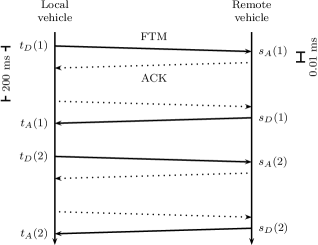
Figure 7: RTT ranging message sequence representing the packets used for evaluating the broadcast algorithm. Compare to Fig. 1 in Section II.

To emulate broadcast ranging, the timestamps of every alternate ranging request packet and every alternate ACK packet were used for processing. An example is shown in Fig. 7. The FTM packets transmitted by the MDP in the car (local vehicle) can be thought of as a proxy for the broadcast DSRC packets from this car and the alternate ACK responses from the static MDP (remote vehicle) can be taken as a proxy for its own broadcast DSRC packets. These are denoted by the solid lines in the figure. Note that the time delay between the FTM request and the alternate ACK’s is on the order of $200$ ms. Thus the effects of clock drifts will be prominently seen in the timestamps and need to be accounted for. Further, this method also helps us to compute distance estimates using RTT based ranging for a baseline comparison by using the ACKs that are immediately sent for every FTM request.

All measurements were carried out at a bandwidth of $80$ MHz which is the largest WiFi band supported by the MDP device. The received signal is then filtered to different lower bandwidths to compare the ranging accuracy as a function of the bandwidth.

The ground-truth device consists of a Novatel GPS module that has a specification of decimeter accuracy in open sky environments. This device was mounted on the vehicle after initially determining the ground truth of the static MDP. The ground-truth device provides location fixes at a rate of $100$ per second. These are downsampled to match the rate of range estimates obtained from the MDP.

An important issue that needed to be resolved when using the ground-truth data was that of the time synchronization between the estimates obtained from the ground-truth device and those from the MDP. Note that the ground-truth device provides measurements timestamped in both its own local clock and in GPS time. The MDP devices however can only provide measurements timestamped in their local clock. To address this synchronization issue, a Python script was used to query the ground-truth device and the MDP board from a single laptop and timestamps were attached to the measurements in this local clock. This provides synchronization up to a few tens of milliseconds which is still comparable to the time duration between the measurements. In the post-processing stage a constant fixed delay between the ground truth and MDP measurements was therefore manually adjusted to minimize the alignment error.

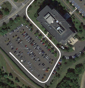
Figure 8: Vehicle trajectory (directed from left to top) plotted on Google Maps. The white dot indicates the position of the static MDP.

The trajectory of the vehicle motion is shown in Fig. 8. The driving environment is largely strong line-of-sight (LOS) except at certain locations where the signal could be blocked by light poles or trees. There are also reflections from the ground and other parked cars that can degrade the estimation accuracy at lower bandwidths. We will see the effects of these in the sections below.

IV-B Comparison of Baseline RTT Scheme and Proposed PBR Scheme

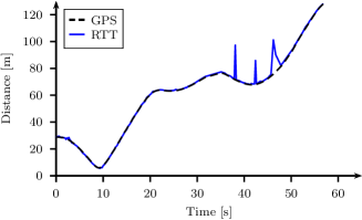
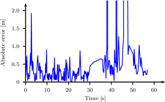
Figure 9: Estimation error for the baseline unicast RTT-ranging approach ($80$ MHz ranging bandwidth).

A comparison of the performance of the baseline RTT scheme with the ground truth at $80$ MHz bandwidth is shown in Fig. 9. There is no averaging or smoothing across time for this plot. One can see that the average errors during the first $20$ s are well within half a meter. There are some large errors mostly between the time instants $35$ s and $50$ s. These correspond to the locations where the car was driving in front of the building as seen in Fig. 8. There are some light poles, trees and other parked cars that contribute to multipath (between $40$ s and $50$ s) and packet loss (between $30$ s and $35$ s). In particular, large multipath errors in this time frame are potentially caused by signal reflection from the building adjacent to the car trajectory.

Figure 10: Estimation error for proposed periodic broadcast ranging (PBR) approach ($80$ MHz ranging bandwidth).

Fig. 10 shows a comparison of the errors between the proposed periodic broadcast ranging (PBR) scheme and the ground truth. One can see that the average errors during the first $20$ s are again well within half a meter. Thus the proposed algorithm is able to estimate the clock drift fairly accurately (recall that these can result in errors of more than $150$ m if not taken care of). The plot looks smoother than RTT due to the local polynomial approximation. Further this approach also eliminates some of the multipath errors due to the local polynomial constraint wherein outliers are rejected. For example, consider the multipath error in Fig. 9 occurring around time $38$ s. This is eliminated in the PBR scheme. However the other multipath errors are not eliminated since these occur in bursts, particularly the one close to $50$ s. Further, the proposed scheme also has errors in certain cases where there are packet losses and the local polynomial prediction can be erroneous. This error is seen at time instants close to $35$ s during which the prediction overshoots the actual trajectory.

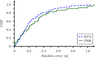
Figure 11: Comparison of estimation error CDFs for unicast (RTT) and broadcast (PBR) approaches over the first $20$ s of vehicle trajectory ($80$ MHz ranging bandwidth).

Fig. 11 shows the error cumulative distribution function (CDF) between the RTT scheme and PBR for the first $20$ s of vehicle trajectory. There is a slight degradation of around $5$ cm for PBR. However the overall average error at the $50$ percentile is around $20$ cm and the $90$ percentile error is well within $1$ m.

IV-C Impact of Ranging Bandwidth

Figure 12: Estimation error CDFs for PBR over the first $20$ s of vehicle trajectory for different ranging bandwidths.

Here we explore the effect of the transmission bandwidth on the ranging accuracy. The received $80$ MHz signal is an OFDM symbol with $256$ frequency tones. This is downsampled to $128$, $64$, and $32$ tones to generate signals occupying $40$ MHz, $20$ MHz, and $10$ MHz, respectively. The time-of-arrival is then estimated based on these downsampled signals. Note that a factor of two reduction in the bandwidth increases the pulse width in time by a factor of two, thereby the accuracy is roughly expected to degrade by a factor of two particularly when we have multipath. This effect is observed in our results as well. Fig. 12 shows a comparison of the error CDFs for the different bandwidths, and one can observe that the accuracy degrades by roughly a factor of two (for example consider the $90$ percentile) with reducing bandwidth.

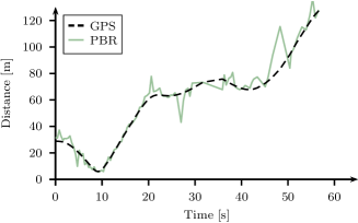
Figure 13: Estimation error for proposed periodic broadcast ranging approach ($10$ MHz ranging bandwidth).

Fig. 13 shows the ranging performance with $10$ MHz transmission bandwidth, which is of interest in the DSRC context. During the first $20$ s, the overall average error at the $50$ percentile is around $1.5$ m as seen from the CDF curves. In the linear section of the vehicle trajectory between $10$ s and $20$ s, the errors are below $1$ m. In this case, there was clear LOS between the two MDPs as opposed to the rest of the trajectory, during which either other parked vehicles or obstructions like light poles resulted in larger errors due to multipath.

V Conclusion

In this work, we investigated the problem of range estimation between vehicles using periodic broadcast transmissions. We proposed a broadcast ranging algorithm that achieves accuracies comparable to unicast RTT based ranging. Thus, the number of message exchanges needed for ranging can be reduced from scaling quadratically in the number of vehicles for the unicast approach to only linearly in the broadcast approach with only a small loss in ranging performance.

Key challenges in broadcast ranging are the presence of clock offsets, clock drifts, and vehicle motion that need to be accounted for. The proposed algorithm is able to efficiently handle these terms and to provide accurate range estimates. We also propose a novel timestamp compression algorithm to minimizes the packet overhead.

References

- [1] U. Niesen, E. N. Ekambaram, J. Jose, and X. Wu, “Vehicular ranging using periodic broadcasts,” in Proc. IEEE VTC, pp. 1–5, Sept. 2015.
- [2] C. R. Drane and C. Rizos, Positioning systems in intelligent transportation systems. Artech House, 1998.
- [3] A. J. Khattak, S. Hallmark, and R. Souleyrette, “Application of light detection and ranging technology to highway safety,” Transport. Res. Rec., vol. 1836, no. 1, pp. 7–15, 2003.
- [4] P. Misra and P. Enge, Global Positioning System: Signals, Measurements and Performance. Ganga-Jamuna Press, second ed., 2006.
- [5] S. A. Golden and S. S. Bateman, “Sensor measurements for Wi-Fi location with emphasis on time-of-arrival ranging,” IEEE Trans. Mobile Comput., vol. 6, pp. 1185–1198, Oct. 2007.
- [6] “IEEE draft standard for information technology–telecommunications and information exchange between systems local and metropolitan area networks–specific requirements part 11: Wireless LAN, medium access control (MAC), and physical layer (PHY) specifications,” 2014.
- [7] “IEEE 1609 - family of standards of wireless access in vehicular environments,” 2014. http://www.standards.its.dot.gov/factsheets/factsheet/80.
- [8] N. Levanon, “Radar principles,” Wiley-Interscience, vol. 1, 1988.
- [9] A. M. Hossain and W.-S. Soh, “A comprehensive study of bluetooth signal parameters for localization,” in Proc. IEEE PIMRC, pp. 1–5, Sept. 2007.
- [10] J.-Y. Lee and R. A. Scholtz, “Ranging in a dense multipath environment using an UWB radio link,” IEEE J. Sel. Areas Commun., vol. 20, pp. 1677–1683, Sept. 2002.
- [11] R. Parker and S. Valaee, “Vehicle localization in vehicular networks,” in Proc. IEEE VTC, pp. 1–5, Sept. 2006.
- [12] N. Alam, A. T. Balaei, and A. G. Dempster, “Range and range-rate measurements using DSRC: facts and challenges,” in Proc. IGNSS, Dec. 2009.
- [13] N. Alam, A. T. Balaie, and A. G. Dempster, “Dynamic path loss exponent and distance estimation in a vehicular network using Doppler effect and received signal strength,” in Proc. IEEE VTC, pp. 1–5, Sept. 2010.
- [14] A. Boukerche, H. A. B. F. Oliveira, E. F. Nakamura, and A. A. F. Loureiro, “Vehicular ad hoc networks: A new challenge for localization-based systems,” Comput. Commun., vol. 31, pp. 2838–2849, July 2008.
- [15] L. Hu and D. Evans, “Localization for mobile sensor networks,” in Proc. ACM MobiCom, pp. 45–57, Sept. 2004.
- [16] S. Lanzisera, D. T. Lin, and K. S. J. Pister, “RF time of flight ranging for wireless sensor network localization,” in Proc. IEEE WISES, pp. 1–12, June 2006.
- [17] B. Denis, J.-B. Pierrot, and C. Abou-Rjeily, “Joint distributed synchronization and positioning in UWB ad hoc networks using TOA,” IEEE Trans. Microw. Theory Techn., vol. 54, pp. 1896–1911, June 2006.
- [18] Y. U. Cao, A. S. Fukunaga, and A. Kahng, “Cooperative mobile robotics: Antecedents and directions,” J. Auton. Robots, vol. 4, pp. 7–27, Mar. 1997.
- [19] J. Djugash, S. Singh, G. Kantor, and W. Zhang, “Range-only SLAM for robots operating cooperatively with sensor networks,” in IEEE ICRA, pp. 2078–2084, May 2006.
- [20] Y. Wang, X. Ma, and G. Leus, “Robust time-based localization for asynchronous networks,” IEEE Trans. Signal Process., vol. 59, pp. 4397–4410, Sept. 2011.
- [21] K.-L. Noh, Q. M. Chaudhari, E. Serpedin, and B. W. Suter, “Novel clock phase offset and skew estimation using two-way timing message exchanges for wireless sensor networks,” IEEE Trans. Commun., vol. 55, pp. 766–777, Apr. 2007.
- [22] Y. Zhou, C. L. Law, Y. L. Guan, and F. Chin, “Indoor elliptical localization based on asynchronous UWB range measurement,” IEEE Trans. Instrum. Meas., vol. 60, pp. 248–257, Jan. 2011.
- [23] R. T. Rajan and A.-J. van der Veen, “Joint ranging and synchronization for an anchorless network of mobile nodes,” IEEE Trans. Signal Process., vol. 63, pp. 1925–1940, Apr. 2015.
- [24] W. S. Cleveland, “Robust locally weighted regression and smoothing scatterplots,” J. Am. Stat. Assoc., vol. 74, pp. 829–836, Dec. 1979.
- [25] K. Ansari, C. Wang, and Y. Feng, “Exploring dependencies of 5.9 GHz DSRC throughput and reliability on safety applications,” in Proc. IEEE APWCS, pp. 448–453, Sept. 2013.