Emergence of charge order in a staggered loop-current phase of cuprate high-temperature superconductors

Abstract

We study the emergence of charge ordered phases within a $\pi$-loop current ($\pi$LC) model for the pseudogap based on a three-band model for underdoped cuprate superconductors. Loop currents and charge ordering are driven by distinct components of the short-range Coulomb interactions: loop currents result from the repulsion between nearest-neighbor copper and oxygen orbitals, while charge order results from repulsion between neighboring oxygen orbitals. We find that the leading $\pi$LC phase has an antiferromagnetic pattern similar to previously discovered staggered flux phases, and that it emerges abruptly at hole dopings $p$ below the van Hove filling. Subsequent charge ordering tendencies in the $\pi$LC phase reveal that diagonal $d$-charge density waves (dCDW) are suppressed by the loop currents while axial order competes more weakly. In some cases we find a wide temperature range below the loop-current transition, over which the susceptibility towards an axial dCDW is large. In these cases, short-range axial charge order may be induced by doping-related disorder. A unique feature of the coexisting dCDW and $\pi$LC phases is the emergence of an incommensurate modulation of the loop currents. If the dCDW is biaxial (checkerboard) then the resulting incommensurate current pattern breaks all mirror and time-reversal symmetries, thereby allowing for a polar Kerr effect.

I Introduction

Charge order is a universal feature of underdoped cuprate high-temperature superconductors. Charge ordered phases lie in close proximity to antiferromagnetic, spin-glass, and superconducting phases, implying a close competition between the different ordering tendencies. This raises the possibility that some or all of the anomalous properties exhibited by the cuprates are due to multiple competing or coexisting electronic phases.

Originally observed by scanning tunneling spectroscopy in Bi-based cupratesHoffman et al. (2002); Kohsaka et al. (2007); Wise et al. (2008), charge order was then inferred to exist also in YBa₂Cu₃O_6+x, e.g. from magneto-transportDaou et al. (2010); Chang et al. (2010, 2011) and magneto-oscillation experiments,Sebastian et al. (2012); Harrison and Sebastian (2012) NMR,Wu et al. (2011, 2013) and x-ray scattering.Ghiringhelli et al. (2012); Chang et al. (2012); Blackburn et al. (2013); Blanco-Canosa et al. (2013); Hücker et al. (2014) More recently, charge order has been found in HgBa₂CuO_4+δDoiron-Leyraud et al. (2013); Barišić et al. (2013); Tabis et al. (2014) and in the electron-doped compound Nd_2-xCe_xCuO₄.da Silva Neto et al. (2015)

The charge order has two distinguishing features: it has modulation wavevectors ${\bf q}$ that lie along the crystalline axes (so-called “axial order”), and it has an approximate $d_{x^{2}-y^{2}}$ internal structure.Kohsaka et al. (2007); Mesaros et al. (2011); Fujita et al. (2014); Comin et al. (2015); Achkar et al. (2014) We therefore adopt the notation $d$-charge density wave (dCDW). In essence, the dCDW can be thought of as a predominant charge transfer between neighboring oxygen $p$-orbitals the amplitude of which is modulated with wavevector ${\bf q}$.Fischer and Kim (2011); Bulut et al. (2013); Atkinson et al. (2015); Fischer et al. (2014)

This dCDW is distinct from the stripe order found in La-based cuprates. While both are strongest near hole dopings of $p=0.12$, stripes are characterized by an entanglement of spin and charge degrees of freedomVojta (2009) that is absent in the dCDW phase;Thampy et al. (2013) additionally, the doping dependence of the density modulations follows an opposite trend in stripe- and charge-ordered materials.Thampy et al. (2013)

Charge order also appears to be distinct from the pseudogap phenomena. Early experiments on YBa₂Cu₃O_6+xGhiringhelli et al. (2012); Chang et al. (2012) and Bi₂Sr_2-xLa_xCuO_6+xComin et al. (2014) found that static charge modulations develop at temperatures $T_{\mathrm{co}}$ close to the pseudogap onset temperature $T^{\ast}$, and this suggested a cause for the partial destruction of the Fermi surface that characterizes the pseudogap. Furthermore, a recent STM study of Bi₂Sr₂CaCu₂O_8+xHamidian et al. (2015) found a connection between the energy scales of the charge order and the pseudogap. However, systematic studies over a wide doping range in YBa₂Cu₃O_6+x have revealed that the onset of the dCDW at $T_{\mathrm{co}}$ varies differently with $p$ than does $T^{\ast}$.Blanco-Canosa et al. (2013); Hücker et al. (2014) In addition, the pseudogap was found insensitive to doping with Zn impurities,Alloul et al. (1991); Zheng et al. (1993, 1996); Alloul et al. (2009) while charge order is rapidly quenched.Blanco-Canosa et al. (2013); Atkinson and Kampf (2015) Finally, the wavevector associated with the dCDW connects tips of the remnant Fermi arcs in the pseudogap phase; this suggests that charge order is an instability of, rather than the cause of, the Fermi arcs;Comin et al. (2014) indeed, theoretical calculations accurately reproduce experimental wavevectors under this assumption.Atkinson et al. (2015); Chowdhury and Sachdev (2014a); Nikšić et al. (2015); Thomson and Sachdev (2015)

Several calculations found instabilities towards dCDW states with ordering wavevectors ${\bf q}$ oriented along the Brillouin zone diagonal (so-called “diagonal order”),Metlitski and Sachdev (2010a, b); Holder and Metzner (2012); Husemann and Metzner (2012); Bejas et al. (2012); Efetov et al. (2013); Bulut et al. (2013); Meier et al. (2013); Sau and Sachdev (2014) in contrast to all the experiments, which find axial order. This discrepancy is resolved by imposing a pseudogap, from which charge order emerges.Chowdhury and Sachdev (2014b); Atkinson et al. (2015); Thomson and Sachdev (2015); Feng et al. (2015) This is not a unique resolution, though: some authors pointed out that axial and diagonal instabilities are close competitors,Sachdev and La Placa (2013); Wang and Chubukov (2014) and in Ref. Yamakawa and Kontani, 2015 the inclusion of Aslamazov-Larkin vertex corrections led to axial order. Empirically, however, it does appear that the pseudogap is a prerequisite for the formation of the dCDW in hole-doped cuprates, since $T_{\mathrm{co}}$ is always less than or equal to $T^{\ast}$. While the underlying reason is unclear, it is possible that short quasiparticle lifetimes at temperatures $T>T^{\ast}$ inhibit the formation of charge order.Bauer and Sachdev (2015)

If a correct description of the dCDW requires a basic understanding of the pseudogap phase, then it is disheartening that the cause of the pseudogap is still unknown. Many recent proposals suggest that the pseudogap is the result of fluctuations of, or competition between, multiple distinct order parametersWang et al. (2015a, b); Hayward et al. (2014); Pépin et al. (2014); Kloss et al. (2015) involving charge and superconductivity. Alternatively, dynamical mean-field calculations find that in the strongly correlated limit, local Coulomb interactions may generate a spectral pseudogap without need for a true phase transition; this is linked to dynamical antiferromagnetic correlations.Kyung et al. (2006); Gunnarsson et al. (2015) However, there is experimental evidence for a true thermodynamic phase transitionShekhter et al. (2013); Ramshaw et al. (2015) at $T^{\ast}$ (although this has been challenged in Ref. Cooper et al., 2014) that terminates at a quantum critical point near $p=0.19.$Castellani et al. (1997); Varma (1997); Tallon and Loram (2001); Taillefer (2010) One prominent suggestion is that the phase below $T^{\ast}$ breaks time-reversal symmetry via microscopic loop currents (LCs) that mayAffleck and Marston (1988); Wang et al. (1990); Chakravarty et al. (2001); Lee et al. (2006); Laughlin (2014) or may notVarma (1997) break the translational symmetry of the lattice.

Considerations about the relationship between the dCDW and the pseudogap recently led us to reexamine the instabilities of multi-orbital models for cuprate superconductors.Bulut et al. (2015) For physically relevant model parameters, we found a leading instability towards a spontaneous $\pi$-loop current ($\pi$LC) phase, in which the circulation of the loop currents alternates to form an orbital antiferromagnet, similar to staggered LC phases that have been proposed in the past.Affleck and Marston (1988); Wang et al. (1990); Chakravarty et al. (2001); Lee et al. (2006); Laughlin (2014) While direct experimental evidence for staggered LC phases in cuprates is still lacking,Mook et al. (2002a, b); Stock et al. (2002); Mook et al. (2004); Sonier et al. (2009) we are nonetheless motivated to study the LC phase for two reasons: first, the persistence with which LC phases are predicted by theory makes it plausible that there exist systems in which LCs are of key importance; second, phase competition of the type found in the cuprates can lead to emergent properties that are distinct from those of the constituent phases.

Here, our starting point is the assumption that the pseudogap follows from a $\pi$LC phase, and we focus on the possible emergence of charge order within this phase. The required formalism is developed in Sec. II, and results thereby obtained are presented in Sec. III. We show in Sec. III.1 that the encountered phases originate from different interactions: the $\pi$LC phase is driven primarily by the Coulomb repulsion between nearest-neighbor copper and oxygen orbitals, while charge ordering is driven by oxygen-oxygen repulsion. In Sec. III.2 we discuss that axial dCDWs can emerge within the $\pi$LC phase while diagonal dCDWs are strongly suppressed. In some cases we find a wide temperature range below the $\pi$LC transition and above the axial dCDW transition, over which the susceptibility towards an axial dCDW is large. In these cases, short-range charge order may be induced by doping-related disorder. One important consequence relates to the Kerr effect that has been measured in YBa₂Cu₃O_6+x;Xia et al. (2008); He et al. (2011) a nonzero signal implies that both time-reversal and mirror symmetries are broken. The spontaneous currents in the $\pi$LC phase break time-reversal symmetry, and mirror symmetries are further broken with the development of the dCDW phase. The coexistence of loop currents and dCDW order therefore offers a candidate case for the observed Kerr rotation.

II Calculations

II.1 Hamiltonian

We adopt a three-band model for the CuO₂ primitive unit cell, as described in Ref. Bulut et al., 2013. The model includes the Cu$d_{x^{2}-y^{2}}$ orbital and the O$p$ orbital from each oxygen that forms a $\sigma$ bond with it; we label these O$p_{x}$ and O$p_{y}$. The noninteracting part of the Hamiltonian is

$$\hat{H}_{0}=\sum_{{\bf k},\sigma}\sum_{\alpha,\beta}c^{\dagger}_{{\bf k}\alpha\sigma}h_{0,\alpha\beta}({\bf k})c_{{\bf k}\beta\sigma},$$ (1)

where $\sigma$ is a spin index and $\alpha$, $\beta$ denote the orbitals. We take the convention that $c_{{\bf k}\beta\sigma}$ is an electron annihilation operator. Because the $\pi$LC phase has a periodicity of two unit cells, we use a supercell comprising two primitive CuO₂ unit cells so that orbital labels run from 1 to 6 (Fig. 1).

We assume that the SU(2) spin invariance is unbroken so that spin-up and spin-down electrons satisfy identical equations of motion. For brevity, we therefore suppress the spin-index except where it is required.

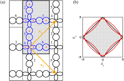
Figure 1: (Color online) Unit supercell and Brillouin zone. (a) The supercell (shaded region) contains two CuO₂ primitive unit cells, with orbitals numbered 1 through 6 as shown. The plus and minus signs indicate the sign convention for the lobes of the Cu$d_{x^{2}-y^{2}}$, O$p_{x}$, and O$p_{y}$ orbitals. The lattice vectors ${\bf a}_{1}$ and ${\bf a}_{2}$ lead to the folded Brillouin zone shown in (b) (shaded region). Backfolded Fermi surfaces are shown for hole filling $p=0.15$ (thick red lines).

The Hamiltonian has diagonal matrix elements $h_{0,\alpha\alpha}({\bf k})$ given by the on-site energies $\epsilon_{d}$ (for $\alpha=1,4$) and $\epsilon_{p}$ (otherwise). The model further includes nearest-neighbor hopping between Cu and O orbitals with amplitude $t_{pd}$, and between adjacent O orbitals with amplitude $t_{pp}$. The Hamiltonian matrix in Eq. (1) is therefore

$${\bf h}_{0}({\bf k})=\left[\begin{array}[]{cc}{\bf h}_{1}({\bf k})&{\bf h}_{2}({\bf k})\\ {\bf h}_{2}({\bf k})^{\dagger}&{\bf h}_{1}({\bf k})\end{array}\right],$$ (2)

where

$${\bf h}_{1}({\bf k}) = \left[\begin{array}[]{ccc}\epsilon_{d}&t_{pd}e^{ik_{y}/2}&-t_{pd}e^{ik_{x}/2}\\ t_{pd}e^{-ik_{y}/2}&\epsilon_{p}&2t_{pp}c_{-}\\ -t_{pd}e^{-ik_{x}/2}&2t_{pp}c_{-}&\epsilon_{p}\end{array}\right],$$ (6)

$${\bf h}_{2}({\bf k}) = \left[\begin{array}[]{ccc}0&-t_{pd}e^{-ik_{y}/2}&t_{pd}e^{-ik_{x}/2}\\ -t_{pd}e^{ik_{y}/2}&0&-2t_{pp}c_{+}\\ t_{pd}e^{ik_{x}/2}&-2t_{pp}c_{+}&0\end{array}\right].$$ (10)

The primitive lattice constant is $a_{0}=1$, and $c_{\pm}=\cos(\frac{k_{x}}{2}\pm\frac{k_{y}}{2})$. The signs of the off-diagonal matrix elements $h_{0,\alpha\beta}({\bf k})$ are determined by the product of signs of the closest lobes of orbitals $\alpha$ and $\beta$, as shown in Fig. 1(a). Because the supercell contains two primitive unit cells, the Brillouin zone is halved and the Fermi surface is folded into the reduced Brillouin zone [Fig. 1(b)].

We consider both on-site and nearest-neighbor Coulomb repulsion, so the interaction has the form

$$\hat{V}=\sum_{i\alpha}U_{\alpha}\hat{n}_{i\alpha\uparrow}\hat{n}_{i\alpha\downarrow}+\frac{1}{2}\sum_{i\alpha\sigma,j\beta\sigma^{\prime}}V_{i\alpha,j\beta}\hat{n}_{i\alpha\sigma}\hat{n}_{j\beta\sigma^{\prime}},$$ (11)

where $i$ and $j$ label supercells, $\alpha$ and $\beta$ label orbitals, $\sigma$ and $\sigma^{\prime}$ label spins, and $\hat{n}_{i\alpha\sigma}=c^{\dagger}_{i\alpha\sigma}c_{i\alpha\sigma}$. The on-site Coulomb interaction $U_{\alpha}$ is $U_{d}$ ($\alpha=1,4$) or $U_{p}$ (otherwise); the nonlocal interaction $V_{i\alpha,j\beta}$ is $V_{pd}$ for nearest-neighbor $p$ and $d$ orbitals, and $V_{pp}$ for adjacent oxygen orbitals.

Following Ref. Bulut et al., 2013 we take $t_{pd}=1$ to be the unit of energy, $t_{pp}=-0.5$, and $\epsilon_{d}-\epsilon_{p}=2.5$. The interaction strengths are $U_{d}=9.0$, $U_{p}=3.0$, $V_{pp}$ varies between 1.0 and 1.3 and $V_{pd}$ between 2.0 and 3.0.

II.2 Hartree-Fock Approximation

Interactions are first treated within a Hartree-Fock (HF) approximation, $\hat{V}\approx\hat{V}_{HF}\equiv\hat{V}_{H}+\hat{V}_{X}$, where the Hartree term is

$$\hat{V}_{H}=\sum_{i\alpha\sigma}U_{\alpha}\hat{n}_{i\alpha\sigma}n_{i\alpha{\overline{\sigma}}}+\sum_{i\alpha\sigma,j\beta\sigma^{\prime}}V_{i\alpha,j\beta}\hat{n}_{i\alpha\sigma}n_{j\beta\sigma^{\prime}},$$ (12)

with ${\overline{\sigma}}\equiv-\sigma$ and $n_{i\alpha\sigma}\equiv\langle\hat{n}_{i\alpha\sigma}\rangle$, and the exchange term is

$$\hat{V}_{X} = -\sum_{i\alpha,j\beta}\sum_{\sigma}c^{\dagger}_{i\alpha\sigma}c_{j\beta\sigma}V_{i\alpha,j\beta}\langle c^{\dagger}_{j\beta\sigma}c_{i\alpha\sigma}\rangle.$$ (13)

Within the HF approximation, the leading instability is to a spin-density wave (SDW) state involving spins on the Cu sites.Bulut et al. (2013) This state is driven by the large local Coulomb interaction $U_{d}$; it is well known that strong correlations suppress the SDW except near half-filling, and we therefore make a restricted HF approximation that preserves the SU(2) invariance of the spins. SU(2) symmetry implies $n_{i\alpha\uparrow}=n_{i\alpha\downarrow}$ and $\langle c^{\dagger}_{j\beta\uparrow}c_{i\alpha\uparrow}\rangle=\langle c^{\dagger}_{j\beta\downarrow}c_{i\alpha\downarrow}\rangle$, so that the HF Hamiltonian is identical for spin-up and spin-down electrons.

Expressing $\hat{V}_{HF}$ in terms of Bloch states (and suppressing the spin index) gives

$$\hat{V}_{HF} = \sum_{{\bf k},{\bf q},\alpha,\beta}P_{\alpha\beta}({\bf k},{\bf q})c^{\dagger}_{{\bf k}+\frac{\bf q}{2}\alpha}c_{{\bf k}-\frac{\bf q}{2}\beta},$$ (14)

where

$$P_{\alpha\beta}({\bf k},{\bf q}) = \frac{1}{N}\sum_{{\bf k}^{\prime}}\sum_{\mu,\nu}\big{\{}\left[U_{\alpha}\delta_{\alpha,\mu}+2V_{\alpha\mu}({\bf q})\right]\delta_{\alpha,\beta}\delta_{\mu,\nu}$$

$$-V_{\alpha\beta}({\bf k}-{\bf k}^{\prime})\delta_{\nu,\beta}\delta_{\mu,\alpha}\big{\}}\langle c^{\dagger}_{{\bf k}^{\prime}-\frac{\bf q}{2}\nu}c_{{\bf k}^{\prime}+\frac{\bf q}{2}\mu}\rangle,$$

is the HF “self-energy” and

$$V_{\alpha\beta}({\bf q})=\sum_{{\bf r}_{\alpha\beta}}e^{i{\bf q}\cdot{\bf r}_{\alpha\beta}}V_{\alpha\beta}({\bf r}_{\alpha\beta}),$$ (16)

with $\{{\bf r}_{\alpha\beta}\}$ the set of intra- and inter-supercell vectors pointing from orbital $\alpha$ to nearest-neighbor orbital $\beta$. Explicit expressions for $V_{\alpha\beta}({\bf q})$ are given in Appendix A.

In the HF approximation, terms proportional to $U_{\alpha}$ contribute only Hartree terms, while the nonlocal terms make both Hartree and exchange contributions. Because our model parameters are chosen phenomenologically to reproduce the cuprate band structure, the homogeneous components of the Hartree and exchange self-energies are implicitly present in the site energies $\epsilon_{d}$ and $\epsilon_{p}$ and hopping matrix elements $t_{pd}$ and $t_{pp}$. To avoid double-counting, we retain only the spatially inhomogeneous components of the interaction self-energy; these will prove responsible for both loop currents and charge order.

It is convenient to decompose the interactions in Eq. (LABEL:eq:P) in a set of basis functions $g^{\ell}_{\alpha\beta}({\bf k})$:

$$\left[U_{\alpha}\delta_{\alpha,\mu}+2V_{\alpha\mu}({\bf q})\right]\delta_{\alpha,\beta}\delta_{\mu,\nu}-V_{\alpha\beta}({\bf k}-{\bf k}^{\prime})\delta_{\nu,\beta}\delta_{\mu,\alpha}$$

$$=\sum_{\ell,\ell^{\prime}}\tilde{V}^{\ell\ell^{\prime}}({\bf q})g^{\ell}_{\alpha\beta}({\bf k})g^{\ell^{\prime}}_{\mu\nu}({\bf k}^{\prime})^{\ast}.$$

(17)

$g^{\ell}_{\alpha\beta}({\bf k})$ are $6\times 6$ matrices in the orbital indices $\alpha$ and $\beta$, with a single nonzero matrix element corresponding to a unique bond or site:

$$g^{\ell}_{\alpha\beta}({\bf k})=e^{i{\bf k}\cdot{\bf r}_{\alpha\beta}}\delta_{\alpha,\alpha_{\ell}}\delta_{\beta,\beta_{\ell}},$$ (18)

where each $\ell$ labels either a directed bond pointing from $\alpha_{\ell}$ to $\beta_{\ell}$, or an orbital when $\alpha_{\ell}=\beta_{\ell}$. There are a total of 38 orbital pairs $(\alpha_{\ell},\beta_{\ell})$, and these are listed in Table 1 in Appendix A, along with the corresponding basis functions. Here, we note that $\ell\in[1,32]$ labels the directed bonds between nearest-neighbor sites, and $\ell\in[33,38]$ labels the six orbitals making up the supercell.

With the decomposition (17), we obtain

$$P_{\alpha\beta}({\bf k},{\bf q}) = \sum_{\ell}\tilde{P}^{\ell}({\bf q})g^{\ell}_{\alpha\beta}({\bf k}),$$ (19)

where

$$\tilde{P}^{\ell}({\bf q})=\frac{1}{N}\sum_{{\bf k}^{\prime}}\sum_{\ell^{\prime},\mu,\nu}\tilde{V}^{\ell\ell^{\prime}}({\bf q})g^{\ell^{\prime}}_{\mu\nu}({\bf k}^{\prime})^{\ast}\langle c^{\dagger}_{{\bf k}^{\prime}-\frac{\bf q}{2}\nu}c_{{\bf k}^{\prime}+\frac{\bf q}{2}\mu}\rangle,$$ (20)

is the self-consistency equation for the HF self-energy for bond $\ell$. To perform an unbiased search for broken-symmetry phases within HF theory, it is most convenient to linearize Eq. (20) so that it acquires the form

$$\tilde{P}^{\ell}({\bf q})=-\sum_{\ell^{\prime},\ell^{\prime\prime}}\tilde{V}^{\ell\ell^{\prime}}({\bf q})\tilde{X}_{0}^{\ell^{\prime}\ell^{\prime\prime}}({\bf q})\tilde{P}^{\ell^{\prime\prime}}({\bf q}).$$ (21)

This step is performed explicitly in the next section.

II.3 Linearized Hartree-Fock Equations

We define a generalized susceptibility that describes the change in $\tilde{P}^{\ell}({\bf q})$ induced by a perturbing field $\tilde{\phi}^{\ell^{\prime}}({\bf q},t)$, where $\ell$ and $\ell^{\prime}$ label either bonds or sites as described above. In the limit of a vanishingly weak perturbation, a phase transition is signalled by a diverging susceptibility eigenvalue.

The general form of the perturbation is

$$\hat{\Phi}(t) = \sum_{m\mu,n\nu}\phi_{m\mu,n\nu}(t)c^{\dagger}_{m\mu}c_{n\nu}$$ (22)

$$= \sum_{{\bf k},{\bf q}}\sum_{\mu\nu}\phi_{\mu\nu}({\bf k},{\bf q},t)c^{\dagger}_{{\bf k}+\frac{\bf q}{2}\mu}c_{{\bf k}-\frac{\bf q}{2}\nu},$$

where $m,n$ label supercells and

$$\phi_{\mu\nu}({\bf k},{\bf q},t)=\frac{1}{N}\sum_{m,n}\phi_{m\mu,n\nu}(t)e^{i{\bf k}\cdot({\bf r}_{n\nu}-{\bf r}_{m\mu})}e^{-i\frac{\bf q}{2}\cdot({\bf r}_{m\mu}+{\bf r}_{n\nu})}.$$ (23)

In this equation, ${\bf k}$ is associated with the relative coordinate connecting orbitals $\mu$ and $\nu$, while ${\bf q}$ is associated with the spatial modulation of the field; a conventional electrostatic potential would have

$$\phi_{\mu\nu}({\bf k},{\bf q},t)=\delta_{\mu,\nu}\phi_{\mu}({\bf q},t).$$ (24)

Provided the perturbation is restricted to on-site and nearest-neighbor terms, Eq. (23) can be decomposed in terms of $g^{\ell}_{\mu\nu}({\bf k})$,

$$\phi_{\mu\nu}({\bf k},{\bf q},t) = \sum_{\ell}\tilde{\phi}^{\ell}({\bf q},t)g^{\ell}_{\mu\nu}({\bf k}).$$ (25)

Then

$$\hat{\Phi}(t)=\sum_{{\bf k},{\bf q}}\sum_{\mu\nu}\sum_{\ell}\tilde{\phi}^{\ell}({\bf q},t)g^{\ell}_{\mu\nu}({\bf k})c^{\dagger}_{{\bf k}+\frac{\bf q}{2}\mu}c_{{\bf k}-\frac{\bf q}{2}\nu}.$$ (26)

Hermiticity of $\hat{\Phi}(t)$ requires for the perturbing fields

$$\tilde{\phi}^{\ell}(-{\bf q},t)=\tilde{\phi}^{{\overline{\ell}}}({\bf q},t)^{\ast},$$ (27)

where $\ell$ and ${\overline{\ell}}$ describe the same bond, but oriented in opposite directions.

The perturbing field induces time-dependent collective excitations $\delta P_{\alpha\beta}({\bf k},{\bf q},t)$ of the self-energy; these feed back into the linear response, so that the total perturbation is

$$\hat{H}^{\prime}(t) = \sum_{{\bf q}}\sum_{\ell}\left[\delta\tilde{P}^{\ell}({\bf q},t)+\tilde{\phi}^{\ell}({\bf q},t)\right]$$ (28)

$$\times\sum_{{\bf k}\mu\nu}g^{\ell}_{\mu\nu}({\bf k})c^{\dagger}_{{\bf k}+\frac{\bf q}{2}\mu}c_{{\bf k}-\frac{\bf q}{2}\nu},$$

where we have expanded $\delta P_{\mu\nu}({\bf k},{\bf q},t)=\sum_{\ell}g^{\ell}_{\mu\nu}({\bf k})\delta\tilde{P}^{\ell}({\bf q},t)$.

A self-consistent expression for $\delta\tilde{P}^{\ell}({\bf q},t)$ is obtained from Kubo’s equation for the first order response of the charge density to $\hat{H}^{\prime}(t)$:

$$\delta\tilde{P}^{\ell}({\bf q},t)=-i\int_{-\infty}^{t}dt^{\prime}\langle[\hat{P}^{\ell}({\bf q},t),\hat{H}^{\prime}(t^{\prime})]\rangle,$$ (29)

where

$$\hat{P}^{\ell}({\bf q})=\frac{1}{N}\sum_{{\bf k}^{\prime}}\sum_{\ell^{\prime},\mu,\nu}\tilde{V}^{\ell\ell^{\prime}}({\bf q})g^{\ell^{\prime}}_{\mu\nu}({\bf k}^{\prime})^{\ast}c^{\dagger}_{{\bf k}^{\prime}-\frac{\bf q}{2}\nu}c_{{\bf k}^{\prime}+\frac{\bf q}{2}\mu}$$ (30)

is the operator form of $\tilde{P}^{\ell}({\bf q})$ [see Eq. (20)]. A straightforward calculation yields

$$\delta\mathbf{\tilde{P}}({\bf q},\omega)=-\mathbf{\tilde{V}}({\bf q})\mathbf{\tilde{X}_{0}}({\bf q},\omega)\left[\delta\mathbf{\tilde{P}}({\bf q},\omega)+\bm{\tilde{\phi}}({\bf q},\omega)\right],$$ (31)

where bold symbols represent matrices and vectors in the $38\times 38$ bond and orbital basis. The bare susceptibility matrix has elements

$$\tilde{X}_{0}^{\ell\ell^{\prime}}({\bf q},\omega) = \frac{1}{N}\sum_{{\bf k}}\sum_{\alpha\beta\mu\nu}g^{\ell}_{\mu\nu}({\bf k})^{\ast}g^{\ell^{\prime}}_{\alpha\beta}({\bf k})$$ (32)

$$\times\sum_{n,n^{\prime}}\Psi_{\mu n}({\bf k}_{+})\Psi^{\ast}_{\alpha n}({\bf k}_{+})\Psi_{\beta n^{\prime}}({\bf k}_{-})\Psi_{\nu n^{\prime}}^{\ast}({\bf k}_{-})$$

$$\times\frac{f(E_{n{\bf k}_{+}})-f(E_{n^{\prime}{\bf k}_{-}})}{\omega+i\delta-E_{n{\bf k}_{+}}+E_{n^{\prime}{\bf k}_{-}}},$$

where ${\bf k}_{\pm}\equiv{\bf k}\pm\frac{\bf q}{2}$, greek symbols are orbital labels, $n$ and $n^{\prime}$ are band indices, and $E_{n{\bf k}}$ and $\Psi_{\mu n}({\bf k})$ are respectively the eigenvalues and eigenvectors of the Hamiltonian ${\hat{H}}_{0}$. In the static limit $\omega\rightarrow 0$ and for a vanishingly weak external potential $\tilde{\phi}^{\ell}({\bf q},\omega)$, Eq. (31) reduces to Eq. (21).

Equation (31) is a $38\times 38$ matrix equation that can be inverted for each ${\bf q}$ and $\omega$ to obtain

$$\delta\mathbf{\tilde{P}}({\bf q},\omega)=-\mathbf{\tilde{V}}({\bf q})\mathbf{\tilde{X}}({\bf q},\omega)\bm{\tilde{\phi}}({\bf q},\omega)$$ (33)

with

$$\mathbf{\tilde{X}}({\bf q},\omega)=\left[\mathbf{1}+\mathbf{\tilde{X}_{0}}({\bf q},\omega)\mathbf{\tilde{V}}({\bf q})\right]^{-1}\mathbf{\tilde{X}_{0}}({\bf q},\omega).$$ (34)

Equation (33) describes the change in the HF self-energy induced by a weak perturbing field.

II.4 Connection to Charge and Current Densities

We denote by $\chi({\bf q})$ the largest eigenvalue of the static susceptibility matrix ${\bf\tilde{X}}({\bf q},0)$. The divergence of $\chi({\bf q})$ as temperature is lowered signals a phase transition. Further information about the resulting phase is obtained from the corresponding eigenvector $\mathbf{\tilde{v}}_{\bf q}$. In particular, both the current and charge density can be obtained from a generalized charge density,

$$\rho_{i\alpha,j\beta}=\langle c^{\dagger}_{i\alpha}c_{j\beta}\rangle,$$ (35)

which is closely related to the HF self-energy by

$$P_{i\alpha,j\beta}=V_{i\alpha,j\beta}\rho_{i\alpha,j\beta}^{\ast}.$$ (36)

For $(i\alpha)=(j\beta)$, $\rho_{i\alpha,j\beta}$ reduces to the single-spin charge density $n_{i\alpha}$, while for nearest-neighbor pairs $(i\alpha)$ and $(j\beta)$, the imaginary part of $\rho_{i\alpha,j\beta}$ gives the probability current along the bond from $(i\alpha)$ to $(j\beta)$,

$$J_{i\alpha,j\beta}=-2t_{i\alpha,j\beta}\mbox{Im}[\rho_{i\alpha,j\beta}].$$ (37)

In Eq. (37), $t_{i\alpha,j\beta}$ is $\pm t_{pd}$ or $\pm t_{pp}$, depending on the bond type, where the sign depends on the relative signs of the closest lobes of orbitals $\alpha$ and $\beta$ in Fig. 1 (thus $t_{i1,i3}=-t_{pd}$; $t_{i5,i6}=+t_{pp}$).

By Fourier transforming Eq. (36) and expanding left and right sides in terms of the basis functions $g^{\ell}_{\alpha\beta}({\bf k})$, we obtain

$$\tilde{P}^{\ell}({\bf q})=\sum_{\ell^{\prime}}\tilde{V}^{\ell\ell^{\prime}}\tilde{\rho}^{\ell^{\prime}}(-{\bf q})^{\ast},$$ (38)

with

$$\tilde{\rho}^{\ell^{\prime}}({\bf q})=\frac{1}{N}\sum_{{\bf k},\alpha,\beta}g^{\ell}_{\alpha\beta}({\bf k})\langle c^{\dagger}_{{\bf k}-\frac{\bf q}{2}\alpha}c_{{\bf k}+\frac{\bf q}{2}\beta}\rangle.$$ (39)

Equation (38) provides a connection between the induced self energy $\delta{\bf\tilde{P}}({\bf q},\omega)$ in Eq. (33) and the corresponding induced change in the generalized charge density $\delta\bm{\tilde{\rho}}({\bf q},\omega)$.

Near the phase transition, the static susceptibility matrix ${\bf\tilde{X}}({\bf q})$ is dominated by the diverging eigenvalue $\chi({\bf q})$, such that

$${\bf\tilde{X}}({\bf q})\approx\chi({\bf q})\mathbf{\tilde{v}}_{\bf q}\mathbf{\tilde{v}}_{\bf q}^{\dagger},$$ (40)

where $\mathbf{\tilde{v}}_{\bf q}$ is the column eigenvector corresponding to $\chi({\bf q})$, $\mathbf{\tilde{v}}_{\bf q}^{\dagger}$ is the transpose conjugate, and the outer product $\mathbf{\tilde{v}}_{\bf q}\mathbf{\tilde{v}}_{\bf q}^{\dagger}$ generates a matrix. Substitution of Eq. (38) into Eq. (33) immediately yields the induced static (generalized) charge density,

$$\delta\bm{\tilde{\rho}}(-{\bf q})^{\ast} = -\mathbf{\tilde{X}}({\bf q})\bm{\tilde{\phi}}({\bf q})$$ (41)

$$= -\varphi_{\bf q}\chi({\bf q})\mathbf{\tilde{v}}_{{\bf q}},$$

where $\varphi_{\bf q}=\mathbf{\tilde{v}}_{{\bf q}}^{\dagger}\cdot\bm{\tilde{\phi}}({\bf q})$ is the projection of the field onto the diverging eigenmode. The hermiticity condition (27), along with a similar condition for ${\bf\tilde{v}}_{\bf q}$ (see Eq. (59) in Appendix B), imposes the constraint $\varphi_{-{\bf q}}=\varphi_{\bf q}$. Then,

$$\delta\rho_{i\alpha,j\beta} = \delta\rho({\bf q})e^{i\frac{\bf q}{2}\cdot({\bf r}_{i\alpha}+{\bf r}_{j\beta})}+\delta\rho(-{\bf q})e^{-i\frac{\bf q}{2}\cdot({\bf r}_{i\alpha}+{\bf r}_{j\beta})}$$ (42)

$$= -\chi({\bf q})\left\{e^{i\frac{\bf q}{2}\cdot({\bf r}_{i\alpha}+{\bf r}_{j\beta})}\varphi_{\bf q}\tilde{v}_{\bf q}^{\overline{\ell}}\right.$$

$$\left.+e^{-i\frac{\bf q}{2}\cdot({\bf r}_{i\alpha}+{\bf r}_{j\beta})}\varphi_{\bf q}^{\ast}\tilde{v}_{\bf q}^{\ell\ast}\right\},$$

where $\ell$ denotes the directed bond from $(i\alpha)$ to $(j\beta)$, and and ${\overline{\ell}}$ denotes the oppositely directed bond. The complex phase of $\phi_{\bf q}$ shifts the density wave spatially, and can therefore be set to zero without loss of generality:

$$\delta\rho_{i\alpha,j\beta} = -\chi({\bf q})\varphi_{\bf q}\left\{e^{i\frac{\bf q}{2}\cdot({\bf r}_{i\alpha}+{\bf r}_{j\beta})}\tilde{v}_{\bf q}^{\overline{\ell}}\right.$$ (43)

$$\left.+e^{-i\frac{\bf q}{2}\cdot({\bf r}_{i\alpha}+{\bf r}_{j\beta})}\tilde{v}_{\bf q}^{\ell\ast}\right\},$$

Real-space patterns shown in the next section are calculated from the portion of Eq. (43) contained in braces.

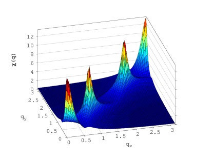
Figure 2: (Color online) Largest eigenvalue of the static susceptibility matrix $\mathbf{\tilde{X}}({\bf q})$ in the normal state at $T=0.010$, $V_{pd}=2.5$, and $p=0.10$.

III Results

III.1 Instabilities of the Normal State

As there are no broken symmetries in the normal high-temperature phase, the HF self-energy generates only a homogeneous renormalization of the model parameters. As discussed above, this homogeneous component is absorbed into the phenomenological model parameters to avoid double-counting. We therefore construct the generalized static susceptibility ${\bf\tilde{X}}({\bf q})$ from the eigenstates of the bare Hamiltonian $\hat{H}_{0}$, defined in Eq. (1).

Figure 2 shows the largest eigenvalue $\chi({\bf q})$ of ${\bf\tilde{X}}({\bf q})$ as a function of ${\bf q}$ close to an instability approached upon cooling. The generalized charge susceptibility allows transitions to charge-, bond-, and current-ordered phases, and the multi-peak structure in Fig. 2 indicates proximity to more than one distinct ordered phase. Because our supercell contains two primitive cells, the points ${\bf q}=(0,0)$ and ${\bf q}=(\pi,\pi)$ are equivalent. Furthermore, peaks at $(q,q)$ and $(\pi-q,\pi-q)$ are related by symmetry. There are, therefore, only two distinct peaks in $\chi({\bf q})$, corresponding to two distinct phases. We use the notation ${\bf q}_{0}=(0,0)$ and ${\bf q}_{1}=(q_{1},q_{1})$ to denote these two kinds of peaks, while ${\bf q}_{2}$ will be used later to denote peaks in the axial direction at $(q_{2},0)$ or $(0,q_{2})$.

For the chosen model parameters there are pronounced peaks at both ${\bf q}_{0}$ and ${\bf q}_{1}$. The peak at ${\bf q}_{0}$ diverges first as $T$ is lowered, and is therefore the leading instability. To determine the nature of the instability, we construct the generalized charge density $\delta\rho_{i\alpha,j\beta}$ induced by an infinitesimally weak field using Eq. (43). The left panel of Fig. 3(a) shows the real part of $\delta\rho_{i\alpha,j\beta}$ for $\alpha\neq\beta$, which is related by Eq. (36) to the bond-strength renormalization. The imaginary parts of $\delta\rho_{i\alpha,j\beta}$ are proportional to the bond currents $\delta J_{i\alpha,j\beta}$, which are shown in the middle panel of Fig. 3(b), while the orbital charge modulations $\delta n_{i\alpha}=\delta\rho_{i\alpha,i\alpha}$ are shown in the right panel. From the figure, it is apparent that the ${\bf q}_{0}$ divergence corresponds to the onset of a staggered loop-current pattern, with no associated charge or bond order. (Note that ${\bf q}_{0}$ is a supercell wavevector, and that the current pattern has wavevector $(\pi,\pi)$ in terms of the primitive unit cell.) This is the same $\pi$LC pattern that was identified previously in Ref. Bulut et al., 2015.

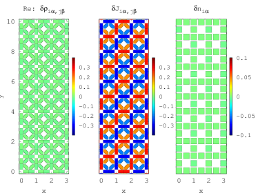
Figure 3: (Color online) Components of the induced generalized charge density $\delta\rho_{i\alpha,j\beta}$ associated with the ${\bf q}_{0}$ eigenmode for the susceptibility shown in Fig. 2. (left) real part of $\delta\rho_{i\alpha,j\beta}$ for $\alpha\neq\beta$, (middle) induced currents $\delta J_{i\alpha,j\beta}$, (right) induced charge modulations $\delta n_{i\alpha}$. Currents with a component of their flow in the positive $x$ direction are deemed positive; currents flowing entirely along the $y$ axis are positive in the positive $y$ direction. $\delta\rho_{i\alpha,j\beta}$ is calculated from Eq. (43) with the prefactor $\chi({\bf q})\varphi_{\bf q}$ set to one; the color scale is therefore arbitrary.

In contrast, Fig. 4 shows that the subdominant peak at ${\bf q}_{1}=(0.84,0.84)$ corresponds to a diagonal dCDW with vanishing orbital currents. The period of this modulation is $2\pi/(0.84\sqrt{2})=5.3$ primitive unit cells, similar to what is found elsewhere, and agrees with the shortest wavevector which connects Fermi surface hotspots. This type of instability has been discussed at length in the literatureMetlitski and Sachdev (2010a, b); Holder and Metzner (2012); Husemann and Metzner (2012); Bejas et al. (2012); Efetov et al. (2013); Bulut et al. (2013); Meier et al. (2013); Sau and Sachdev (2014).

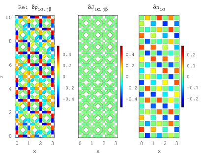
Figure 4: (Color online) As in Fig. 3, but for the peak in Fig. 2 at ${\bf q}_{1}=(0.84,0.84)$. This case corresponds to a diagonal dCDW with no circulating currents.

While the details of the competition between the $\pi$LC and charge ordered phases depend on the band structure, a simple picture emerges concerning the interactions driving these two phases. In Fig. 5 $\chi({\bf q})$ is plotted along the Brillouin zone diagonal as functions of both $V_{pd}$ and $V_{pp}$: Fig. 5(a) shows that $\chi({\bf q}_{0})$ is enhanced by increasing $V_{pd}$ while Fig. 5(b) shows that $\chi({\bf q}_{1})$ is enhanced by increasing $V_{pp}$. This demonstrates that $V_{pd}$ drives the $\pi$LC phase while $V_{pp}$ drives the dCDW.

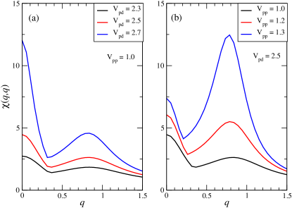
Figure 5: (Color online) Effects of $V_{pd}$ and $V_{pp}$ on the susceptibility eigenvalue $\chi({\bf q})$. Plots show cuts along the Brillouin zone diagonal, ${\bf q}=(q,q)$. Results are for (a) fixed $V_{pp}=1.0$ and varying $V_{pd}$; (b) fixed $V_{pd}=2.5$ and varying $V_{pp}$. $V_{pd}$ enhances the loop-current susceptibility at ${\bf q}_{0}$, while $V_{pp}$ enhances the charge susceptibility peak at ${\bf q}_{1}$. Results are for $T=0.025$ and hole density $p=0.12$.

Figures 6 and 7 show the dependence of the $\pi$LC phase on various model parameters. We caution that factors not included in our calculations must inevitably affect the phase diagram quantitatively. Notably, strong correlations renormalize the electronic effective mass, which grows as the hole doping $p$ is reduced, and the enhanced spin fluctuations make a further doping-dependent contribution to the self-energy.

Figure 6 shows the phase diagram which follows from the susceptibility calculations within the symmetry-unbroken normal state. This figure illustrates the particular significance of the van Hove filling $p_{\mathrm{vH}}$, which denotes the crossover from a hole-like Fermi surface at $p<p_{\mathrm{vH}}$ to an electron-like Fermi surface at $p>p_{\mathrm{vH}}$. It was found previouslyBulut et al. (2013) that in the region $p<p_{\mathrm{vH}}$, the leading charge instability is to a diagonal dCDW, while for $p>p_{\mathrm{vH}}$ the tendency is towards either a ${\bf q}=(0,0)$ nematic phase with an intra-unit cell charge redistribution or an axial dCDW. Figure 6 shows that the $\pi$LC phase is restricted to the region $p<p_{\mathrm{vH}}$, where it competes with the diagonal dCDW phase.

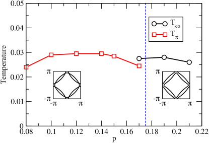
Figure 6: (Color online) Phase diagram of the three-band model from linear response theory. The figure shows the doping dependence of the leading instability temperature of the generalized susceptibility ${\bf\tilde{X}}({\bf q})$. The van Hove hole density $p_{\mathrm{vH}}$ is indicated by a vertical dashed line, and representative Fermi surfaces for $p<p_{\mathrm{vH}}$ and $p>p_{\mathrm{vH}}$ are shown in the insets. The leading charge instability is towards a diagonal dCDW for $p=0.17$, and to a translationally invariant nematic phase consisting of an intra-unit cell transfer of charge between adjacent oxygen orbitals for $p>p_{\mathrm{vH}}$.Bulut et al. (2013) Results are for $V_{pd}=3.0$, $V_{pp}=1.0$.

This result is confirmed by self-consistent HF calculations of the $\pi$LC phase diagram in Fig. 7. For these calculations, the self-energy has the periodicity of the supercell, and Eq. (20) can be expressed simply in terms of the eigenvalues $E_{n{\bf k}}$ and eigenfunctions $\Psi_{\alpha n}({\bf k})$ of the HF Hamiltonian, $\hat{H}_{HF}=\hat{H}_{0}+\hat{V}_{HF}$. The ${\bf q}={\bf 0}$ self-energy for bond $\ell$ is

$$\tilde{P}^{\ell} = \sum_{\ell^{\prime}}\tilde{V}^{\ell\ell^{\prime}}\frac{1}{N}\sum_{\alpha\beta{\bf k}^{\prime}}g^{\ell^{\prime}}_{\alpha\beta}({\bf k}^{\prime})^{\ast}\Psi^{\ast}_{\beta n}({\bf k}^{\prime})\Psi_{\alpha n}({\bf k}^{\prime})f(E_{n{\bf k}^{\prime}}).$$

Because the real part of Eq. (LABEL:eq:Ptilde2) yields a homogeneous shift of the model parameters, we have retained only the imaginary part of $\tilde{P}^{\ell}$ in the self-consistency cycle.

Figure 7 shows the amplitude of the current $J_{pd}$ along the $p$-$d$ bonds in the $\pi$LC phase. The current is measured in units of $et_{pd}/\hbar$, so $J_{pd}=0.01$ corresponds to a current of $\sim 1$ $\mu$A if $t_{pd}=500$ meV. The current sets in at $p_{vH}$ and its amplitude grows as hole doping is further reduced. The termination of the $\pi$LC phase at $p\approx p_{\mathrm{vH}}$ is robust, as it is nearly independent of $V_{pd}$, and it is generally consistent with a recent experimental conclusion that the pseudogap phase is bounded by a Lifshitz transition.Benhabib et al. (2015) However, the $p$-dependence of $J_{pd}$ is expected to be affected by strong correlations. In mean-field theory, the spectral gap associated with the $\pi$LC phase is proportional to the current amplitude. The HF self-energy Eq. (36) on the $p$-$d$ bonds, which determines both the spectral gap and $T_{\pi}$, is proportional to $V_{pd}$ and the generalized density $\rho_{pd}$ between $p$ and $d$ orbitals, while the current in Eq. (37) is proportional to $t_{pd}$ and $\rho_{pd}$. In the simplest picture, $t_{pd}\propto p$ so that the loop current amplitudes are renormalized downwards by strong correlations relative to the HF self-energy. This is similar to an effect predicted for strongly correlated superconductors: in conventional superconductors, the superconducting $T_{c}$ is proportional to the superconducting gap $\Delta$; however, superfluid stiffness, and therefore $T_{c}$, is strongly reduced by strong correlations while the pairing gap remains large.Anderson (1987); Zhang et al. (1988); Gros (1988); Paramekanti et al. (2004); Haule and Kotliar (2007) This suggests that the trends shown in Fig. 7(b) qualitatively capture the spectral gap but not the LC amplitude.

The $\pi$LC phase stops abruptly at low $p$ at a value that does depend on $V_{pd}$; such a lower bound is not seen experimentally; however, the low-doping region of the phase diagram is complicated by strong correlations, the onset of a spin-glass phase, and by disorderAlvarez and Dagotto (2008); Atkinson (2007) which are beyond the scope of our current calculations.

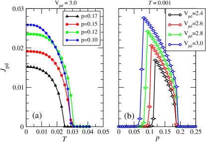
Figure 7: (Color online) Self-consistent Hartree-Fock results for the orbital current as a function of hole filling $p$, temperature $T$, and interaction $V_{pd}$. The current $J_{pd}$ along the $p$-$d$ bond is shown as a function of (a) $T$ for $V_{pd}=3.0$ and (b) $p$ for various $V_{pd}$ at $T=0.001$. The ratio of the $p$-$p$ and $p$-$d$ bond currents is $J_{pp}/J_{pd}=0.32$, independent of $T$, $p$, and $V_{pd}$. It was previously found to depend on the ratio of $t_{pp}/t_{pd}$.Bulut et al. (2015) The current is in units of $et_{pd}/\hbar$, with $e$ the electron charge.

III.2 Charge Instabilities in the Loop-Current State

To determine the leading instability within the $\pi$LC phase, we plot the $T$-dependence of the leading eigenvalue $\chi({\bf q})$ in Fig. 8 at ${\bf q}_{0}$ (loop current), ${\bf q}_{1}$ (diagonal dCDW), and ${\bf q}_{2}$ (axial dCDW). The susceptibility and its eigenvalues are now calculated using the self-consistent HF Hamiltonian for the $\pi$LC phase. We focus on the region $p<p_{\mathrm{vH}}$, where loop currents are found, and results are shown at five different dopings between $p=0.10$ and $p=0.17$. For reference, the Fermi surface and $T$-dependence of $J_{pd}$ are also shown for each doping.

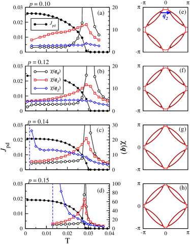
Figure 8: (Color online) Temperature evolution of the peaks in $\chi({\bf q})$ at ${\bf q}_{0}$, ${\bf q}_{1}$, and ${\bf q}_{2}$ at four different fillings: (a) $p=0.10$, (b) $p=0.12$, (c) $p=0.14$, (d) $p=0.15$ The corresponding mean-field current along the $p$-$d$ bond is also shown in each figure (left scale). The three wavevectors are ${\bf q}_{0}=(0,0)$, ${\bf q}_{1}=(q_{1},q_{1})$, ${\bf q}_{2}=(q_{2},0)$, where $q_{1}$ and $q_{2}$ are the peak positions along diagonal and axial directions. Fermi surfaces corresponding to the different hole fillings are shown in (e)-(h) for the normal state (red lines) and for the $\pi$LC state (black lines). As shown in (e), the axial wavevector connects tips of the hole pockets in the $\pi$LC phase.

At temperatures above $T_{\pi}$, $\chi({\bf q})$ grows at all three ${\bf q}$ values as $T$ is reduced. For $p\leq 0.15$, $\chi({\bf q}_{0})$ diverges first, signaling the onset of the $\pi$LC phase at $T_{\pi}$; $\chi({\bf q}_{0})$ then collapses rapidly in the ordered phase below $T_{\pi}$. For all hole densities in Fig. 8, the subleading peak is at ${\bf q}_{1}$ for $T>T_{\pi}$, indicating a tendency towards a diagonal dCDW. This peak at ${\bf q}_{1}$ is reduced by the onset of loop currents, however, which demonstrates a strong competition between diagonal dCDW and $\pi$LC order.

In contrast, there is only a weak competition between axial dCDW and $\pi$LC order. Above $T_{\pi}$, $\chi({\bf q}_{2})$ has positive curvature characteristic of growth towards a divergence; however, all curves show an inflection point slightly below $T_{\pi}$ indicating that the onset of loop currents interrupts this divergence. Rather than being suppressed by loop currents, $\chi({\bf q}_{2})$ tends to saturate below $T_{\pi}$ at a constant value [Figs. 8(a) and (b)], which can be an order of magnitude larger than at high $T$. At some doping levels [Figs. 8(c) and (d)], $\chi({\bf q}_{2})$ actually diverges below $T_{\pi}$, signaling the onset of an axially oriented dCDW. This is shown for $p=0.15$ in Fig. 9, which shows the emergence of strong peaks at ${\bf q}_{2}=(q_{2},0)$ and symmetry related points. The corresponding eigenmode is illustrated in Fig. 10: there is a pronounced transfer of charge between O$p$ orbitals, with an amplitude that is modulated along the $y$-axis [right panel of Fig. 10]. There is a smaller charge modulation on the Cu sites, amounting to $\sim 15\%$ of the O$p$ modulations. This is similar to the axial dCDW found previously for a phenomenological pseudogap modelAtkinson et al. (2015), and both the ordering wavevector and $d$-wave like form factor of the charge modulations are consistent with experiments.Comin et al. (2015); Fujita et al. (2014)

Concomitantly, the real part of $\delta\rho_{i\alpha,j\beta}$ (left panel in Fig. 10) inhomogeneously modulates the effective hopping strength, while the imaginary part corresponds to an incommensurate modulation of the bond current (middle panel in Fig. 10). We have checked that this incommensurate current pattern conserves charge at each vertex of the lattice. Indeed, it is straightforward to construct such a modulated current pattern by hand by requiring that current is conserved at each vertex. Current conservation at the Cu site at position $(m,n)a_{0}$, where $a_{0}$ is the primitive lattice constant, requires that the current coming in along the $x$-axis must be carried out along the $y$-axis, namely

$$\sum_{s=\pm 1}\left[I_{x}(m+\frac{s}{2},n)+I_{y}(m,n+\frac{s}{2})\right]=0\,.$$ (45)

For a modulation wavevector ${\bf q}_{2}=(0,q_{2})$, this constraint implies,

$$I_{x}(m+\frac{1}{2},n)=I_{0}(-1)^{n+m}\cos(q_{2}na_{0}+\theta),$$ (46)

where $\theta$ is an arbitrary constant phase, and

$$I_{y}(m,n+\frac{1}{2})=-I_{0}(-1)^{n+m}\frac{\cos[q_{2}(n+\frac{1}{2})a_{0}+\theta]}{\cos(q_{2}a_{0}/2)}.$$ (47)

Current conservation along the oxygen-oxygen bonds is simpler, as it requires only that the current is constant around each loop within a plaquette.

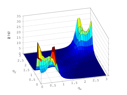
Figure 9: (Color online) Largest eigenvalue of the susceptibility matrix in the $\pi$LC phase. Results are at $p=0.15$ for $V_{pd}=3.0$, $V_{pp}=1.0$, and at $T=0.021$.

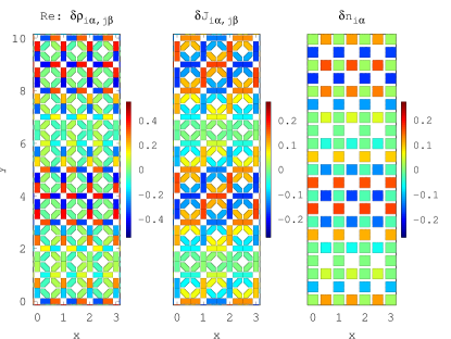
Figure 10: (Color online) Left panel: induced shift in the real part of $\langle c^{\dagger}_{i\alpha}c_{j\beta}\rangle$, middle panel: the bond current, and left panel: the charge density. Parameters are as in Fig. 9. The charge modulations on the Cu sites are $\sim 15\%$ of those on the O sites.

The weak competition between axial dCDW and $\pi$LC order has implications for the role of disorder. While the growth of critical diagonal dCDW fluctuations is interrupted at $T_{\pi}$, $\chi({\bf q}_{2})$ in some instances saturates below $T_{\pi}$ at values that are substantially enhanced relative to the noninteracting case (where $\chi({\bf q})$ is a number of order 1). Figure 8(c), for example, is characterized by a wide temperature range below $T_{\pi}$ where $\chi({\bf q}_{2})$ is more than an order of magnitude larger than in the noninteracting case. In this case crystalline disorder, for example due to dopant atoms, will induce short-range charge correlations with a strong ${\bf q}_{2}$ component even well above the charge-ordering transition at $T_{\mathrm{co}}=0.002$.

This is consistent with what is observed in the cuprates, where static short-range dCDW correlations develop at temperatures as high as $\sim 150$ K;Ghiringhelli et al. (2012); Chang et al. (2012) and true long-range dCDW order (with correlation lengths large enough to observe magneto-oscillation effects) only occurs at much lower temperatures, of order $\sim 50$ K.Wu et al. (2011)

Finally, we note that the generalized susceptibility diverges simultaneously at symmetry-related points along the $x$- and $y$-directions (Fig. 9). Our linearized equations cannot determine whether uniaxial order, with ordering wavector $(q_{2},0)$ or $(0,q_{2})$, or biaxial (checkerboard) order in which both Fourier peaks are simultaneously present, is energetically preferred. Experimentally, domains of uniaxial order are seen in Bi₂Sr₂CaCu₂O_8+x,Fujita et al. (2014) while biaxial order is implied by magneto-oscillation experiments in YBa₂Cu₃O_6+x.Sebastian et al. (2012)

In our calculations, the biaxial dCDW state is of particular interest because it breaks all mirror symmetries of the lattice, and coupled with the time-reversal symmetry breaking of the $\pi$LC phase should generate a polar Kerr effect,Wang et al. (2014); Gradhand et al. (2015) similar to what has been measured in both YBa₂Cu₃O_6+xXia et al. (2008) and Pb_0.55Bi_1.5Sr_1.6La_0.4CuO_6+δ.He et al. (2011) This mechanism should be distinguished from other proposals involving microscopic currents: in Refs. Wang et al., 2014 and Gradhand et al., 2015, the currents run along the edges of charge stripes, while in Ref. Sharma et al., 2015 a combination of staggered loop currents and $d_{xy}$ bond order is proposed to explain the polar Kerr measurements. It remains unclear whether nanodomains of uniaxial order might also lead to a polar Kerr effect in our model.

IV Conclusions

Motivated by the recent discovery of ubiquitous charge order within the pseudogap phase of underdoped cuprate superconductors, we have studied the development of $d$-charge density waves from within a pseudogap phase generated by a staggered $\pi$-loop current. Our main finding is that the $\pi$LC phase competes strongly with the dominant diagonal dCDW phase, and may weaken it sufficiently that axial dCDW order emerges as the leading charge instability. The resulting charge structure is consistent with x-ray scattering and STM experiments. A unique feature of the coexistence of dCDW and $\pi$LC order is the emergence of an incommensurate modulation of the loop current amplitude, illustrated in Fig. 10. If the dCDW has a checkerboard structure, then the resulting incommensurate current pattern breaks both mirror and time-reversal symmetries and should generate a polar Kerr effect.

Appendix A Hartree-Fock Approximation and Basis Functions

In this appendix, we discuss technical details of our treatment of the interactions in the Hartree-Fock approximation. First, we give an explicit form for $V_{\alpha\beta}({\bf q})$, defined by Eq. (16). Referring to Fig. 1, we obtain

$$V_{12}({\bf q}) = V_{45}({\bf q})=V_{24}({\bf q})=V_{51}({\bf q})=V_{pd}e^{iq_{y}/2}$$

$$V_{21}({\bf q}) = V_{54}({\bf q})=V_{42}({\bf q})=V_{15}({\bf q})=V_{pd}e^{-iq_{y}/2}$$

$$V_{13}({\bf q}) = V_{34}({\bf q})=V_{46}({\bf q})=V_{61}({\bf q})=V_{pd}e^{iq_{x}/2}$$

$$V_{31}({\bf q}) = V_{43}({\bf q})=V_{64}({\bf q})=V_{16}({\bf q})=V_{pd}e^{-iq_{x}/2}$$

$$V_{23}({\bf q}) = V_{32}({\bf q})=V_{56}({\bf q})=V_{65}({\bf q})$$

$$= 2V_{pp}\cos\left(\frac{q_{x}-q_{y}}{2}\right)$$

$$V_{26}({\bf q}) = V_{62}({\bf q})=V_{53}({\bf q})=V_{35}({\bf q})$$ (48)

$$= 2V_{pp}\cos\left(\frac{q_{x}+q_{y}}{2}\right),$$

with all other matrix elements zero.

The correspondence between the basis function $\ell$ and the orbital label is given in Table 1. From this table, we learn for example that

$$g^{5}_{\alpha\beta}({\bf k})=e^{ik_{y}/2}\delta_{\alpha,4}\delta_{\beta,5}.$$ (49)

For this basis,

$$\tilde{V}^{\ell\ell^{\prime}}({\bf q})=\left\{\begin{array}[]{ll}-V_{pd}&\ell=\ell^{\prime};\ell\in[1,16]\\ -V_{pp}&\ell=\ell^{\prime};\ell\in[17,32]\\ U_{d}&\ell=\ell^{\prime}=33,36\\ U_{p}&\ell=\ell^{\prime}=34,35,37,38\\ 2V_{\alpha\beta}({\bf q})&\ell\neq\ell^{\prime};\,\ell,\ell^{\prime}\in[33,38]\\ 0&\mbox{otherwise}\end{array}\right.$$ (50)

For the matrix elements containing $V_{\alpha\beta}({\bf q})$, $\ell$ determines $\alpha$ and $\ell^{\prime}$ determines $\beta$, with the connection given by Table 1.

$\ell$	$\alpha_{\ell}$	$\beta_{\ell}$	$g^{\ell}({\bf k})$	$\ell$	$\alpha_{\ell}$	$\beta_{\ell}$	$g^{\ell}({\bf k})$	$\ell$	$\alpha_{\ell}$	$\beta_{\ell}$	$g^{\ell}({\bf k})$	${\bf r}_{\alpha\rightarrow\beta}$	$\ell$	$\alpha_{\ell}$	$\beta_{\ell}$	$g^{\ell}({\bf k})$	${\bf r}_{\alpha\rightarrow\beta}$	$\ell$	$\alpha_{\ell}$	$\beta_{\ell}$	$g^{\ell}({\bf k})$
1	1	2	$e^{ik_{y}/2}$	9	2	1	$e^{-ik_{y}/2}$	17	2	3	$e^{i(k_{x}-k_{y})/2}$	$+{\bf a}_{2}/2$	25	3	2	$e^{-i(k_{x}-k_{y})/2}$	$-{\bf a}_{2}/2$	33	1	1	1
2	1	3	$e^{ik_{x}/2}$	10	3	1	$e^{-ik_{x}/2}$	18	2	3	$e^{-i(k_{x}-k_{y})/2}$	$-{\bf a}_{2}/2$	26	3	2	$e^{i(k_{x}-k_{y})/2}$	$+{\bf a}_{2}/2$	34	2	2	1
3	1	5	$e^{-ik_{y}/2}$	11	5	1	$e^{ik_{y}/2}$	19	2	6	$e^{i(k_{x}+k_{y})/2}$	$+{\bf a}_{1}/2$	27	6	2	$e^{-i(k_{x}+k_{y})/2}$	$-{\bf a}_{1}/2$	35	3	3	1
4	1	6	$e^{-ik_{x}/2}$	12	6	1	$e^{ik_{x}/2}$	20	2	6	$e^{-i(k_{x}+k_{y})/2}$	$-{\bf a}_{1}/2$	28	6	2	$e^{i(k_{x}+k_{y})/2}$	$+{\bf a}_{1}/2$	36	4	4	1
5	4	5	$e^{ik_{y}/2}$	13	5	4	$e^{-ik_{y}/2}$	21	5	6	$e^{i(k_{x}-k_{y})/2}$	$+{\bf a}_{2}/2$	29	6	5	$e^{-i(k_{x}-k_{y})/2}$	$-{\bf a}_{2}/2$	37	5	5	1
6	4	6	$e^{ik_{x}/2}$	14	6	4	$e^{-ik_{x}/2}$	22	5	6	$e^{-i(k_{x}-k_{y})/2}$	$-{\bf a}_{2}/2$	30	6	5	$e^{i(k_{x}-k_{y})/2}$	$+{\bf a}_{2}/2$	38	6	6	1
7	4	2	$e^{-ik_{y}/2}$	15	2	4	$e^{ik_{y}/2}$	23	3	5	$e^{i(k_{x}+k_{y})/2}$	$+{\bf a}_{1}/2$	31	5	3	$e^{-i(k_{x}+k_{y})/2}$	$-{\bf a}_{1}/2$
8	4	3	$e^{-ik_{x}/2}$	16	3	4	$e^{ik_{x}/2}$	24	3	5	$e^{-i(k_{x}+k_{y})/2}$	$-{\bf a}_{1}/2$	32	5	3	$e^{i(k_{x}+k_{y})/2}$	$+{\bf a}_{1}/2$

Table 1: The basis functions $g^{\ell}_{\alpha\beta}({\bf k})=g^{\ell}({\bf k})\delta_{\alpha,\alpha_{\ell}}\delta_{\beta,\beta_{\ell}}$. The index $\ell$ labels the different basis functions, and each $\ell$ corresponds to a unique pair of orbitals $\alpha_{\ell}$ and $\beta_{\ell}$ for which $g^{\ell}_{\alpha_{\ell}\beta_{\ell}}({\bf k})$ is nonzero. In this basis, and for $\ell\in[1,32]$, the quantity $\tilde{P}^{\ell}$ defined in Eq. (20) is simply the bond self-energy $P_{i\alpha,j\beta}$ for nearest neighbor sites $i\alpha$, $j\beta$. For $\ell\in[17,32]$, there are two nearest-neighbor pairs for each $\alpha,\beta$, and to remove the ambiguity, the table shows the vector ${\bf r}_{\alpha\rightarrow\beta}$ pointing from $\alpha$ to $\beta$. The basis functions with $\ell\in[33,38]$ are used to represent the Hartree self-energies.

Appendix B Symmetries of the Susceptibility

B.1 Hermiticity of $\mathbf{\tilde{X}}({\bf q})$

From Eq. (32), we obtain the relationship for the static susceptibility

$$\tilde{X}_{0}^{\ell\ell^{\prime}}({\bf q})^{\ast}=\tilde{X}_{0}^{\ell^{\prime}\ell}({\bf q}),$$ (51)

or, in matrix notation, $\mathbf{\tilde{X}_{0}}({\bf q})^{\dagger}=\mathbf{\tilde{X}_{0}}({\bf q})$. Since $\mathbf{\tilde{V}}({\bf q})^{\dagger}=\mathbf{\tilde{V}}({\bf q})$, it also follows that

$$\mathbf{\tilde{X}}({\bf q})^{\dagger}=\mathbf{\tilde{X}}({\bf q}).$$ (52)

B.2 Relation between $\mathbf{\tilde{X}}({\bf q})$ and $\mathbf{\tilde{X}}(-{\bf q})$

It also follows from Eq. (32) that

$$\tilde{X}_{0}^{\ell\ell^{\prime}}(-{\bf q})=\tilde{X}_{0}^{{\overline{\ell}}^{\prime}{\overline{\ell}}}({\bf q})=\left[\tilde{X}_{0}^{{\overline{\ell}}{\overline{\ell}}^{\prime}}({\bf q})\right]^{\ast}.$$ (53)

where ${\overline{\ell}}$ represents the same bond as $\ell$, but oriented in the opposite sense. Let ${\bf T}$ be the unitary matrix that swaps bonds to the opposite orientation, we obtain the matrix representation ${\bf\tilde{X}_{0}}(-{\bf q})={\bf T\tilde{X}_{0}}({\bf q}){\bf T}^{\dagger}$. Because

$${\bf\tilde{V}}({\bf q})={\bf T\tilde{V}}({\bf q}){\bf T}^{\dagger};\qquad{\bf\tilde{V}}(-{\bf q})={\bf\tilde{V}}({\bf q})^{\ast}$$ (54)

it also happens that

$${\bf\tilde{X}}(-{\bf q})={\bf T\tilde{X}}({\bf q})^{\ast}{\bf T}^{\dagger}.$$ (55)

For the labeling of the bonds shown in Table 1,

$${\bf T}=\left[\begin{array}[]{cc|cc|c}{\bf 0}_{8\times 8}&{\bf 1}_{8\times 8}&{\bf 0}_{8\times 8}&{\bf 0}_{8\times 8}&{\bf 0}_{8\times 6}\\ {\bf 1}_{8\times 8}&{\bf 0}_{8\times 8}&{\bf 0}_{8\times 8}&{\bf 0}_{8\times 8}&{\bf 0}_{8\times 6}\\ \hline\cr{\bf 0}_{8\times 8}&{\bf 0}_{8\times 8}&{\bf 0}_{8\times 8}&{\bf 1}_{8\times 8}&{\bf 0}_{8\times 6}\\ {\bf 0}_{8\times 8}&{\bf 0}_{8\times 8}&{\bf 1}_{8\times 8}&{\bf 0}_{8\times 8}&{\bf 0}_{8\times 6}\\ \hline\cr{\bf 0}_{6\times 8}&{\bf 0}_{6\times 8}&{\bf 0}_{6\times 8}&{\bf 0}_{6\times 8}&{\bf 1}_{6\times 6}\end{array}\right]$$ (56)

Note that ${\bf T}^{\dagger}={\bf T}$ in this case.

B.3 Eigenvectors of $\mathbf{\tilde{X}}({\bf q})$

Equation (55) implies that the eigenvalue equation, $\mathbf{\tilde{X}}({\bf q}){\bf v}_{\bf q}=\chi({\bf q}){\bf v}_{\bf q}$, transforms as

$$\mathbf{T\tilde{X}}({\bf q})^{\ast}\mathbf{T^{\dagger}T}{\bf v}_{\bf q}^{\ast} = \chi({\bf q}){\bf Tv}_{\bf q}^{\ast}$$ (57)

$$\mathbf{\tilde{X}}(-{\bf q})\mathbf{T}{\bf v}_{\bf q}^{\ast} = \chi({\bf q}){\bf Tv}_{\bf q}^{\ast}.$$ (58)

Because $\chi(-{\bf q})=\chi({\bf q})$, it follows that ${\bf Tv}_{\bf q}^{\ast}=e^{i\theta}{\bf v}_{-{\bf q}}$, where $\theta$ is an arbitrary phase. Without loss of generality, we take $\theta=0$ and

$${\bf Tv}_{\bf q}^{\ast}={\bf v}_{-{\bf q}}.$$ (59)

B.4 Simplification of the equation for $\delta\rho_{i\alpha,j\beta}$

Equation (41) gives the induced generalized charge density

$$\delta\bm{\tilde{\rho}}({\bf q})=-\mathbf{\tilde{X}}(-{\bf q})^{\ast}\bm{\tilde{\phi}}(-{\bf q})^{\ast}.$$ (60)

Using the symmetry relations above along with the hermiticity condition (27), Eq. (60) becomes

$$\bm{\tilde{\rho}}({\bf q})=-{\bf T\tilde{X}}({\bf q})\bm{\tilde{\phi}}({\bf q}).$$ (61)

Letting $\ell$ correspond to the bond $(i\alpha,j\beta)$,

$$\delta\rho_{i\alpha,j\beta} = \delta\tilde{\rho}^{\ell}({\bf q})e^{i\frac{\bf q}{2}\cdot({\bf r}_{i\alpha}+{\bf r}_{j\beta})}+\delta\tilde{\rho}^{\ell}(-{\bf q})e^{-i\frac{\bf q}{2}\cdot({\bf r}_{i\alpha}+{\bf r}_{j\beta})}$$ (62)

$$= -e^{i\frac{\bf q}{2}\cdot({\bf r}_{i\alpha}+{\bf r}_{j\beta})}\left[{\bf T\tilde{X}({\bf q})\tilde{\phi}({\bf q})}\right]^{\ell}$$

$$-e^{-i\frac{\bf q}{2}\cdot({\bf r}_{i\alpha}+{\bf r}_{j\beta})}\left[{\bf\tilde{X}({\bf q})^{\ast}\tilde{\phi}({\bf q})^{\ast}}\right]^{\ell}.$$

If $\bm{\tilde{\phi}}({\bf q})$ is proportional to an eigenvector of ${\bf\tilde{X}}({\bf q})$ with real eigenvalue $\chi({\bf q})$, then

$$\delta\rho_{i\alpha,j\beta} = -\chi({\bf q})\Big{\{}e^{i\frac{\bf q}{2}\cdot({\bf r}_{i\alpha}+{\bf r}_{j\beta})}\left[{\bf T}\bm{\tilde{\phi}}({\bf q})\right]^{\ell}$$

$$+e^{-i\frac{\bf q}{2}\cdot({\bf r}_{i\alpha}+{\bf r}_{j\beta})}\left[\bm{\tilde{\phi}}({\bf q})^{\ast}\right]^{\ell}\Big{\}}$$

$$= -\chi({\bf q})\left\{e^{i\frac{\bf q}{2}\cdot({\bf r}_{i\alpha}+{\bf r}_{j\beta})}\tilde{\phi}^{\overline{\ell}}({\bf q})\right.$$

$$\left.+e^{-i\frac{\bf q}{2}\cdot({\bf r}_{i\alpha}+{\bf r}_{j\beta})}\tilde{\phi}^{\ell}({\bf q})^{\ast}\right\}.$$

Taking $\tilde{\phi}^{\overline{\ell}}({\bf q})=\varphi_{\bf q}v_{\bf q}^{\overline{\ell}}$, we obtain Eq. (42).

References

- Hoffman et al. (2002) J. E. Hoffman, E. W. Hudson, K. M. Lang, V. Madhavan, H. Eisaki, S. Uchida, and J. C. Davis, Science 295, 466 (2002).
- Kohsaka et al. (2007) Y. Kohsaka, C. Taylor, K. Fujita, A. Schmidt, C. Lupien, T. Hanaguri, M. Azuma, M. Takano, H. Eisaki, H. Takagi, et al., Science 315, 1380 (2007).
- Wise et al. (2008) W. D. Wise, M. C. Boyer, K. Chatterjee, T. Kondo, T. Takeuchi, H. Ikuta, Y. Wang, and E. W. Hudson, Nat. Phys. 4, 696 (2008).
- Daou et al. (2010) R. Daou, J. Chang, D. LeBoeuf, O. Cyr-Choinière, F. Laliberté, N. Doiron-Leyraud, B. J. Ramshaw, R. Liang, D. A. Bonn, W. N. Hardy, et al., Nature 463, 519 (2010).
- Chang et al. (2010) J. Chang, R. Daou, C. Proust, D. LeBoeuf, N. Doiron-Leyraud, F. Laliberté, B. Pingault, B. J. Ramshaw, R. Liang, D. A. Bonn, et al., Phys. Rev. Lett. 104, 057005 (2010).
- Chang et al. (2011) J. Chang, N. Doiron-Leyraud, F. Laliberté, R. Daou, D. LeBoeuf, B. Ramshaw, R. Liang, D. Bonn, W. Hardy, C. Proust, et al., Phys. Rev. B 84, 014507 (2011).
- Sebastian et al. (2012) S. E. Sebastian, N. Harrison, and G. Lonzarich, Rep. Prog. Phys. 75, 102501 (2012).
- Harrison and Sebastian (2012) N. Harrison and S. E. Sebastian, New J. Phys. 14, 095023 (2012).
- Wu et al. (2011) T. Wu, H. Mayaffre, S. Krämer, M. Horvatić, C. Berthier, W. N. Hardy, R. Liang, D. A. Bonn, and M.-H. Julien, Nature 477, 191 (2011).
- Wu et al. (2013) T. Wu, H. Mayaffre, S. Krämer, M. Horvatić, C. Berthier, P. L. Kuhns, A. P. Reyes, R. Liang, W. N. Hardy, D. A. Bonn, et al., Nat. Comm. 4, 2113 (2013).
- Ghiringhelli et al. (2012) G. Ghiringhelli, M. Le Tacon, M. Minola, S. Blanco-Canosa, C. Mazzoli, N. B. Brookes, G. M. De Luca, A. Frano, D. G. Hawthorn, F. He, et al., Science 337, 821 (2012).
- Chang et al. (2012) J. Chang, E. Blackburn, A. T. Holmes, N. B. Christensen, J. Larsen, J. Mesot, R. Liang, D. A. Bonn, W. N. Hardy, A. Watenphul, et al., Nat. Phys. 8, 871 (2012).
- Blackburn et al. (2013) E. Blackburn, J. Chang, M. Hücker, A. T. Holmes, N. B. Christensen, R. Liang, D. A. Bonn, W. N. Hardy, U. Rütt, O. Gutowski, et al., Phys. Rev. Lett. 110, 137004 (2013).
- Blanco-Canosa et al. (2013) S. Blanco-Canosa, A. Frano, T. Loew, Y. Lu, J. Porras, G. Ghiringhelli, M. Minola, C. Mazzoli, L. Braicovich, E. Schierle, et al., Phys. Rev. Lett. 110, 187001 (2013).
- Hücker et al. (2014) M. Hücker, N. B. Christensen, A. T. Holmes, E. Blackburn, E. M. Forgan, R. Liang, D. A. Bonn, W. N. Hardy, O. Gutowski, M. v. Zimmermann, et al., Phys. Rev. B 90, 054514 (2014).
- Doiron-Leyraud et al. (2013) N. Doiron-Leyraud, S. Lepault, O. Cyr-Choinière, B. Vignolle, G. Grissonnanche, F. Laliberté, J. Chang, N. Barišić, M. K. Chan, L. Ji, et al., Phys. Rev. X 3, 021019 (2013).
- Barišić et al. (2013) N. Barišić, S. Badoux, M. K. Chan, C. Dorow, W. Tabis, B. Vignolle, G. Yu, J. Béard, X. Zhao, C. Proust, et al., Nature Physics 9, 761 (2013).
- Tabis et al. (2014) W. Tabis, Y. Li, M. Le Tacon, L. Braicovich, A. Kreyssig, M. Minola, G. Dellea, E. Weschke, M. J. Veit, M. Ramazanoglu, et al., Nature Communications 5, 1 (2014).
- da Silva Neto et al. (2015) E. H. da Silva Neto, R. Comin, F. He, R. Sutarto, Y. Jiang, R. L. Greene, G. A. Sawatzky, and A. Damascelli, Science 347, 282 (2015).
- Mesaros et al. (2011) A. Mesaros, K. Fujita, H. Eisaki, S. Uchida, J. C. Davis, S. Sachdev, J. Zaanen, M. J. Lawler, and E.-A. Kim, Science 333, 426 (2011).
- Fujita et al. (2014) K. Fujita, M. H. Hamidian, S. D. Edkins, C. K. Kim, Y. Kohsaka, M. Azuma, M. Takano, H. Takagi, H. Eisaki, S.-i. Uchida, et al., Proc. Nat. Acad. Sci. 111, E3026 (2014).
- Comin et al. (2015) R. Comin, R. Sutarto, F. He, E. d. S. Neto, L. Chauviere, A. Frano, R. Liang, W. N. Hardy, D. Bonn, Y. Yoshida, et al., Nature Materials 14], 796 (2015).
- Achkar et al. (2014) A. J. Achkar, F. He, R. Sutarto, C. McMahon, M. Zwiebler, M. Hücker, G. D. Gu, R. Liang, D. A. Bonn, W. N. Hardy, et al. (2014), eprint http://arxiv.org/abs/1409.6787.
- Fischer and Kim (2011) M. H. Fischer and E.-A. Kim, Phys. Rev. B 84, 144502 (2011).
- Bulut et al. (2013) S. Bulut, W. A. Atkinson, and A. P. Kampf, Phys. Rev. B 88, 155132 (2013).
- Atkinson et al. (2015) W. A. Atkinson, A. P. Kampf, and S. Bulut, New Journal of Physics 17, 013025 (2015).
- Fischer et al. (2014) M. H. Fischer, S. Wu, M. Lawler, A. Paramekanti, and E.-A. Kim, New J. Phys. 16, 093057 (2014).
- Vojta (2009) M. Vojta, Advances in Physics 58, 699 (2009).
- Thampy et al. (2013) V. Thampy, S. Blanco-Canosa, M. García-Fernández, M. P. M. Dean, G. D. Gu, M. Föerst, B. Keimer, M. L. Tacon, S. B. Wilkins, and J. P. Hill, Phys. Rev. B 88, 024505 (2013).
- Comin et al. (2014) R. Comin, A. Frano, M. M. Yee, Y. Yoshida, H. Eisaki, E. Schierle, E. Weschke, R. Sutarto, F. He, A. Soumyanarayanan, et al., Science 343, 390 (2014).
- Hamidian et al. (2015) M. H. Hamidian, S. D. Edkins, C. K. Kim, J. C. S. Davis, A. P. Mackenzie, H. Eisaki, S. Uchida, M. J. Lawler, E. A. Kim, S. Sachdev, et al. (2015).
- Alloul et al. (1991) H. Alloul, P. Mendels, H. Casalta, J. F. Marucco, and J. Arabski, Phys. Rev. Lett. 67, 3140 (1991).
- Zheng et al. (1993) G.-Q. Zheng et al., J. Phys. Soc. Jpn. 62, 2591 (1993).
- Zheng et al. (1996) G.-Q. Zheng, T. Odaguchi, Y. Kitaoka, K. Asayama, Y. Kodama, K. Mizuhashi, and S. Uchida, Physica C 263, 367 (1996).
- Alloul et al. (2009) H. Alloul, J. Bobroff, M. Gabay, and P. J. Hirschfeld, Rev. Mod. Phys. 81, 45 (2009).
- Atkinson and Kampf (2015) W. A. Atkinson and A. P. Kampf, Phys. Rev. B 91, 104509 (2015).
- Chowdhury and Sachdev (2014a) D. Chowdhury and S. Sachdev, Phys. Rev. B 90, 245136 (2014a).
- Nikšić et al. (2015) G. Nikšić, D. K. Sunko, and S. Barišić, Physica B: Physics of Condensed Matter pp. 1–4 (2015).
- Thomson and Sachdev (2015) A. Thomson and S. Sachdev, Physical Review B 91 (2015).
- Metlitski and Sachdev (2010a) M. A. Metlitski and S. Sachdev, Phys. Rev. B 82, 075128 (2010a).
- Metlitski and Sachdev (2010b) M. Metlitski and S. Sachdev, New J. Phys. 12, 105007 (2010b).
- Holder and Metzner (2012) T. Holder and W. Metzner, Phys. Rev. B 85, 165130 (2012).
- Husemann and Metzner (2012) C. Husemann and W. Metzner, Phys. Rev. B 86, 085113 (2012).
- Bejas et al. (2012) M. Bejas, A. Greco, and H. Yamase, Phys. Rev. B 86, 224509 (2012).
- Efetov et al. (2013) K. B. Efetov, H. Meier, and C. Pépin, Nat. Phys. 9, 442 (2013).
- Meier et al. (2013) H. Meier, M. Einenkel, C. Pépin, and K. B. Efetov, Phys. Rev. B 88, 020506 (2013).
- Sau and Sachdev (2014) J. D. Sau and S. Sachdev, Phys. Rev. B 89, 075129 (2014).
- Chowdhury and Sachdev (2014b) D. Chowdhury and S. Sachdev, Phys. Rev. B 90, 134516 (2014b).
- Feng et al. (2015) S. Feng, D. Gao, and H. Zhao (2015), eprint http://arxiv.org/abs/1510.05384.
- Sachdev and La Placa (2013) S. Sachdev and R. La Placa, Phys. Rev. Lett. 111, 027202 (2013).
- Wang and Chubukov (2014) Y. Wang and A. Chubukov, Phys. Rev. B 90, 035149 (2014).
- Yamakawa and Kontani (2015) Y. Yamakawa and H. Kontani, Physical review letters 114, 257001 (2015).
- Bauer and Sachdev (2015) J. Bauer and S. Sachdev, Phys. Rev. B 92, 085134 (2015).
- Wang et al. (2015a) Y. Wang, D. F. Agterberg, and A. Chubukov, Physical review letters 114, 197001 (2015a).
- Wang et al. (2015b) Y. Wang, D. F. Agterberg, and A. Chubukov, Physical Review B 91 (2015b).
- Hayward et al. (2014) L. E. Hayward, D. G. Hawthorn, R. G. Melko, and S. Sachdev, Science 343, 1336 (2014).
- Pépin et al. (2014) C. Pépin, V. S. de Carvalho, T. Kloss, and X. Montiel, Phys. Rev. B 90, 195207 (2014).
- Kloss et al. (2015) T. Kloss, X. Montiel, and C. Pépin, Phys. Rev. B 91, 205124 (2015).
- Kyung et al. (2006) B. Kyung, S. S. Kancharla, D. Senechal, A. M. S. Tremblay, M. Civelli, and G. Kotliar, Phys. Rev. B 73, 165114 (2006).
- Gunnarsson et al. (2015) O. Gunnarsson, T. Schäfer, J. P. F. LeBlanc, E. Gull, J. Merino, G. Sangiovanni, G. Rohringer, and A. Toschi, Physical review letters 114, 236402 (2015).
- Shekhter et al. (2013) A. Shekhter, B. J. Ramshaw, R. Liang, W. N. Hardy, D. A. Bonn, F. F. Balakirev, R. D. McDonald, J. B. Betts, S. C. Riggs, and A. Migliori, Nature 498, 75 (2013).
- Ramshaw et al. (2015) B. J. Ramshaw, S. E. Sebastian, R. D. McDonald, J. Day, B. S. Tan, Z. Zhu, J. B. Betts, R. Liang, D. A. Bonn, W. N. Hardy, et al., Science 348, 317 (2015).
- Cooper et al. (2014) J. R. Cooper, J. W. Loram, I. Kokanović, J. G. Storey, and J. L. Tallon, Phys. Rev. B 89, 201104 (2014).
- Castellani et al. (1997) C. Castellani, C. Di Castro, and M. Grilli, Z. Phys. B 103, 137 (1997).
- Varma (1997) C. M. Varma, Phys. Rev. B 55, 14554 (1997).
- Tallon and Loram (2001) J. L. Tallon and J. W. Loram, Physica C 349, 53 (2001).
- Taillefer (2010) L. Taillefer, Annual Review of Condensed Matter Physics 1, 51 (2010).
- Affleck and Marston (1988) I. Affleck and J. B. Marston, Phys. Rev. B 37, 3774 (1988).
- Wang et al. (1990) Z. Wang, G. Kotliar, and X.-F. Wang, Phys. Rev. B 42, 8690 (1990).
- Chakravarty et al. (2001) S. Chakravarty, R. B. Laughlin, D. K. Morr, and C. Nayak, Phys. Rev. B 63, 094503 (2001).
- Lee et al. (2006) P. A. Lee, N. Nagaosa, and X.-G. Wen, Rev. Mod. Phys. 78, 17 (2006).
- Laughlin (2014) R. Laughlin, Phys. Rev. Lett. 112, 017004 (2014).
- Bulut et al. (2015) S. Bulut, A. P. Kampf, and W. A. Atkinson (2015), eprint http://arxiv.org/abs/1503.08896.
- Mook et al. (2002a) H. A. Mook, P. Dai, S. M. Hayden, A. Hiess, J. W. Lynn, S.-H. Lee, and F. Doğan, Phys. Rev. B 66, 144513 (2002a).
- Mook et al. (2002b) H. Mook, P. Dai, and F. Doğan, Physical review letters 88, 097004 (2002b).
- Stock et al. (2002) C. Stock, W. Buyers, Z. Tun, R. Liang, D. Peets, D. Bonn, W. Hardy, and L. Taillefer, Physical Review B 66, 024505 (2002).
- Mook et al. (2004) H. A. Mook, P. Dai, S. M. Hayden, A. Hiess, S.-H. Lee, and F. Dogan, Phys. Rev. B 69, 134509 (2004).
- Sonier et al. (2009) J. Sonier, V. Pacradouni, S. Sabok-Sayr, W. Hardy, D. Bonn, R. Liang, and H. Mook, Physical review letters 103, 167002 (2009).
- Xia et al. (2008) J. Xia, E. Schemm, G. Deutscher, S. A. Kivelson, D. A. Bonn, W. N. Hardy, R. Liang, W. Siemons, G. Koster, M. M. Fejer, et al., Physical review letters 100, 127002 (2008).
- He et al. (2011) R.-H. He, M. Hashimoto, H. Karapetyan, J. D. Koralek, J. P. Hinton, J. P. Testaud, V. Nathan, Y. Yoshida, H. Yao, K. Tanaka, et al., Science 331, 1579 (2011).
- Benhabib et al. (2015) S. Benhabib, A. Sacuto, M. Civelli, I. Paul, M. Cazayous, Y. Gallais, M. A. Méasson, R. D. Zhong, J. Schneeloch, G. D. Gu, et al., Physical review letters 114, 147001 (2015).
- Anderson (1987) P. W. Anderson, Science 235, 1196 (1987).
- Zhang et al. (1988) F. C. Zhang, C. Gros, T. M. Rice, and H. Shiba, Superconductor Science and Technology 1, 36 (1988).
- Gros (1988) C. Gros, Phys. Rev. B 38, 931 (1988).
- Paramekanti et al. (2004) A. Paramekanti, M. Randeria, and N. Trivedi, Phys. Rev. B 70, 054504 (2004).
- Haule and Kotliar (2007) K. Haule and G. Kotliar, Phys. Rev. B 76, 104509 (2007).
- Alvarez and Dagotto (2008) G. Alvarez and E. Dagotto, Phys. Rev. Lett. 101, 177001 (2008).
- Atkinson (2007) W. Atkinson, Physical Review B 75, 024510 (2007).
- Wang et al. (2014) Y. Wang, A. Chubukov, and R. Nandkishore, Physical Review B 90, 205130 (2014).
- Gradhand et al. (2015) M. Gradhand, I. Eremin, and J. Knolle, Physical Review B 91, 1 (2015).
- Sharma et al. (2015) G. Sharma, S. Tewari, P. Goswami, V. M. Yakovenko, and S. Chakravarty, pp. 1–5 (2015), eprint http://arxiv.org/abs/1503.07174.