Optimal Prediction by Cellular Signaling Networks

Abstract

Living cells can enhance their fitness by anticipating environmental change. We study how accurately linear signaling networks in cells can predict future signals. We find that maximal predictive power results from a combination of input-noise suppression, linear extrapolation, and selective readout of correlated past signal values. Single-layer networks generate exponential response kernels, which suffice to predict Markovian signals optimally. Multilayer networks allow oscillatory kernels that can optimally predict non-Markovian signals. At low noise, these kernels exploit the signal derivative for extrapolation, while at high noise, they capitalize on signal values in the past that are strongly correlated with the future signal. We show how the common motifs of negative feedback and incoherent feed-forward can implement these optimal response functions. Simulations reveal that E. coli can reliably predict concentration changes for chemotaxis, and that the integration time of its response kernel arises from a trade-off between rapid response and noise suppression.

The ability to respond and adapt to changing environments is a defining property of life. Single-celled organisms employ a range of response strategies, tailored to the environmental fluctuations they encounter. Gradual changes in osmolarity, pH or available nutrients are sensed and responded to adiabatically. In this regime, the sensory performance as measured by the mutual information between stimulus and response, limits the achievable growth rate Bergstrom and Lachmann (2005); Taylor et al. (2007); Bialek (2012). In contrast, when environmental changes are rapid and unpredictable, sensing may be futile, since any response would come too late. Here, phenotypic heterogeneity can help by providing a subpopulation of pre-adapted cells Balaban et al. (2004). An intermediate regime exists where environmental fluctuations occur with some regularity, on the cellular response time scale. It is then possible and desirable for the cell to predict the future environment, in order to initiate a response ahead of time. When the cellular response takes a finite time $\tau$ to become effective, the predictive mutual information between the current sensory output and the environment $\tau$ later, limits growth sup . Sensing strategies that leverage correlations of a stimulus with future environmental changes have indeed been observed, and re-evolved experimentally Mitchell et al. (2009); Tagkopoulos et al. (2008).

This raises the question of what makes a cellular network an optimal predictor, rather than instantaneous reporter, of the environment. Intuitively, to predict, one should rely on the most up-to-date information, i.e. respond to the current input. However, cells often sense non-Markovian (NM) signals, whose past trajectories could add useful information. Intriguingly, in such cases, sensory networks often react not instantaneously but instead more slowly, on the time scale of the signal Kaupp et al. (2008); Valencia et al. (2012).

A slow network time integrates the input signal, which may dampen the response, but can also enhance the estimate of the current input signal by filtering noise from, e.g., receptor-ligand binding Berg and Purcell (1977); Bialek and Setayeshgar (2005); Govern and ten Wolde (2012); Mehta and Schwab (2012); Kaizu et al. (2014); Govern and ten Wolde (2014). Moreover, a slow response may enhance prediction by building a memory of the signal history which is informative about the future signal. What features of signal and response then make a non-instantaneous response beneficial for prediction?

Here, we study how the accuracy of prediction depends on the noise and correlations in the input, the forecast interval, and the design of the response system. We find that single-layer responders, such as push-pull networks, can improve prediction by responding slowly. This not only allows noise averaging, but also enables reading out past signals that are more correlated with the future signal than the current signal is. Multilayer networks can further enhance prediction via non-monotonic response functions tailored to the input. They can optimally predict low-noise signals by exploiting the signal derivative, and high-noise signals by coherently summing informative past signal values. This can be imlemented via negative feedback. Finally, we perform simulations of E. coli bacteria that chemotax in spatially varying concentration fields. The simulations reveal that E. coli chemotaxis relies on predicting future concentration changes. They suggest that the optimal integration time of the kernel arises as a compromise between the benefit of responding quickly to the most recent concentration values, and the need to filter input noise.

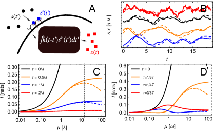
Figure 1: Biochemical prediction. (A) A sensory network (black box) with output $x$ (red) senses an extracellular ligand $s$ (black) via noisy ligand-bound receptors $\ell$ (blue). (B) Example traces (solid lines) of Markovian ($\lambda=1$, red) and non-Markovian (NM) signals $s$ ($\omega=1$, $\eta=4,2,0.5$, downwards), yielding outputs $x$ of exponential responders with $\mu=1$ (dashed). Predictive information $I[x,s_{\tau}]$ in nats ($\ln 2\leavevmode\nobreak\ \mathrm{nats}=1\leavevmode\nobreak\ \mathrm{bit}$) for Markovian signals (C) and NM signals with damping $\eta=1/2$ (D), as a function of the speed $\mu$ of an exponential responder, for different prediction intervals $\tau$, and for noise level $\vartheta=0$ (solid lines) and $\vartheta=0.1$ (dashed lines). Dotted line in (C) denotes $\mu_{\rm ti}$.

Consider a general sensory network which responds to a time-varying extracellular signal by binding ligand molecules, relaying the signal via intermediate species, and finally producing an output species (Fig. 1A). Its prediction capability depends on both responder and input properties. Concerning the input, prediction fundamentally requires that past inputs contain information about the future, i.e. the signal’s conditional probability density $p(s(t+\tau)|s(t),s(t^{\prime}),\dots)$ really depends on the signal values at $t>t^{\prime}>\cdots$. For Markovian input, the only dependence is on $s(t)$, and perfect instantaneous readout of $s(t)$ would in fact be the optimal prediction strategy for all future $s(t+\tau)$ sup . However, in the presence of input noise $\xi$, arising from, e.g, receptor-ligand binding, the responder senses the degraded signal $\ell(t)=s(t)+\xi(t)$. Then even for Markovian $s$, the added noise makes $p(s(t+\tau)|\ell(t),\ell(t^{\prime}),\dots)$ dependent on past values $\ell(t^{\prime}),\dots$, since they help determine the current input $s(t)$ by averaging over the noise $\xi$, and then from $s(t)$ the future $s(t+\tau)$. Thus a slow response can help prediction of any noisy signal via the mechanism of time integration (which also improves accuracy for constant, noisy signals Berg and Purcell (1977); Bialek and Setayeshgar (2005); Govern and ten Wolde (2012); Mehta and Schwab (2012); Kaizu et al. (2014); Govern and ten Wolde (2014, 2014); Aquino et al. (2014)). As detailed below, for NM signals, another prediction mechanism exists: A responder with memory enables readout of additional information from past signals $s(t^{\prime}),\dots$, improving predictions by exploiting signal correlations.

We take the input signal $s(t)$ to be stationary Gaussian, characterized by $\langle{}s(t^{\prime})s(t^{\prime}+t)\rangle=\sigma_{s}^{2}r_{s}(t)$ where $r_{s}$ denotes the normalized autocorrelation function, and $\sigma_{s}$, the signal amplitude. For Markovian processes, $r_{s}(t)=\exp(-\lambda t)$. A family of NM signals can be generated via a harmonic oscillator defined by $\partial_{\omega t}q=p,\;\partial_{\omega t}p=-q-\eta p+\sqrt{2\eta}\psi$ with unit white noise $\psi$, by letting $s\equiv q$, see Fig. 1B. The damping parameter $\eta$ controls the signal statistics: in the overdamped regime $\eta>2$, $r_{s}(t)$ is monotonically decreasing, while for $\eta<2$ it is oscillatory with period approaching $T=2\pi/\omega$; in both cases, the signal $s$ obeys Gaussian statistics. This family of signals allows analytical results and interpolates from Markovian to non-Markovian, long-range correlated, oscillatory signals. We model input noise as white, $\langle{}\xi(t)\xi(t^{\prime})\rangle=\sigma_{s}^{2}\vartheta^{2}\delta(t-t^{\prime})$, where $\vartheta$ is the relative noise strength.

Concerning the responder, we focus on linear signaling networks Heinrich et al. (2002); Govern and ten Wolde (2012) which afford analytical results and often describe information transmission remarkably well Tănase-Nicola et al. (2006); Ziv et al. (2007); de Ronde et al. (2010). Since we are interested in how prediction depends on the correlations and noise in the input, we consider responders in the deterministic limit. The output $x(t)=\int_{-\infty}^{t}k(t-t^{\prime})\ell(t^{\prime})dt^{\prime}$ of the network is then determined by its linear response function $k(t)$.

The predictive power of a signal-responder system is measured in a rigorous and biologically relevant way sup by the predictive mutual information $I[x,s_{\tau}]=\big{\langle}\log\frac{p(x,s_{\tau})}{p(x)p(s_{\tau})}\big{\rangle}$ between the current output $x(t)$ and the future input $s_{\tau}\equiv s(t+\tau)$. Since $x$ is jointly Gaussian with the input, the predictive information reduces to a function $I[x,s_{\tau}]=-\frac{1}{2}\log(1-r_{xs_{\tau}}^{2})$ of the input-output correlation coefficient

$$r_{xs_{\tau}} =\frac{\Psi(\tau)}{[\Sigma+\Xi]^{1/2}}.$$ (1)

The overlap integral $\Psi(\tau)\equiv\int_{0}^{\infty}k(t)r_{s}(t+\tau)dt$ is the part of the normalized output variance $\sigma^{2}_{x}/\sigma^{2}_{s}$ that is correlated with the prediction target $s_{\tau}$. The denominator splits $\sigma^{2}_{x}/\sigma^{2}_{s}$ into contributions from past signal, $\Sigma\equiv\int_{0}^{\infty}k(t)r_{s}(t-t^{\prime})k(t^{\prime})dtdt^{\prime}$, and past noise $\Xi\equiv\vartheta^{2}\int_{0}^{\infty}k(t)^{2}dt$ sup .

We first consider a push-pull network, consisting of a single layer in which the output $x$ is directly activated by the receptor. It is characterized by an exponential kernel $k(t)\propto\exp(-\mu t)$ with response speed $\mu$. Fig. 1C shows how accurately such a network can predict Markovian signals, as measured by the predictive information $I$, obtained analytically from Eq. 1 sup . Without input noise ($\vartheta\to 0$), the fastest responders maximize the accuracy $I$, as expected. When including input noise, there exists an optimal response speed $\mu_{\text{ti}}=(2\lambda/\vartheta^{2}+\lambda^{2})^{1/2}$, independent of $\tau$, and approaching $\mu_{\text{ti}}\to\lambda$ for high noise Hinczewski and Thirumalai (2014). The optimum arises from a trade-off between rapid tracking of the input and noise averaging sup .

Fig. 1D shows $I$ for exponential responders predicting oscillatory ($\eta=0.5$) NM signals. As before, input noise disfavors the fastest responders. Interestingly, however, a finite response speed can be optimal even when there is no input noise ($\vartheta=0$): For prediction intervals above about a quarter period, frequency-matched responders with $\mu_{*}\simeq\omega$ (obtained numerically sup ), perform best.

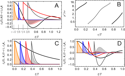
Figure 2: Prediction by optimizing correlations. (A) NM autocorrelation $r_{s}$ at $\eta=0.5$ (black). Optimally predictive exponential kernels $k(t-\tau)$ at noise level $\vartheta=0.25$ for $\tau/T=1/8,1/4,3/8$ as indicated (orange, blue, red, gray, respectively); with corresponding overlap integrands $r_{s}(t)k(t-\tau)$ (shaded). (B) Optimal $\mu_{*}$ vs. prediction interval for these parameters. Solid, dashed lines: positive, negative $sx$ correlation, respectively. (C) As (A) at the same $\tau$ values but for the globally optimal kernels $k_{*}$ and overdamped signal $\eta=4$. (D) As (C) but for underdamped signal at $\eta=0.5$.

The optimal $\mu_{*}$ is not an effect of simple time integration but rather results from exploiting the oscillatory signal correlations. When the forecast interval $\tau\ll T$, $r_{xs_{\tau}}^{2}$ is maximized by increasing the overlap $\Psi(\tau)^{2}$ via a short kernel $k$ that samples high values of the input correlation function $r_{s}$, Fig. 2A,B. The optimal kernels never become instantaneous, however, since that would strongly increase $\Xi$. As $\tau$ increases, $\mu_{*}$ initially increases: $k(t)$ decays faster so that it continues to overlap with the positive lobe of $r_{s}(t+\tau)$; input and output remain positively correlated. Surprisingly, beyond a critical prediction interval $\tau_{c}\simeq 0.22T$, $\mu_{*}$ drops discontinuously (Fig. 2B, solid to dashed line). The response now integrates the negative lobe of $r_{s}$, anticorrelating output and input (Fig. 2A). Effectively, the output $x$ lags behind the input $s$ by an amount $\Lambda$, so that the current output $x(t)$ reflects the past input $s(t-\Lambda)$ rather than the current input $s(t)$. This enhances prediction, because the past signal $s(t-\Lambda)$ is more (anti)correlated with, and hence more informative about, the future $s(t+\tau)$ than the present signal $s(t)$ is, as shown by the non-monotonic signal autocorrelation function: $r_{s}(\Lambda+\tau)^{2}>r_{s}(\tau)^{2}$ (cf. Fig. S2 in sup ). The optimal response speed $\mu_{*}$ is such that $\tau+\Lambda\simeq T/2$; the response kernel $k(t)$ then probes $r_{s}$ around its minimum, maximizing the squared overlap $\Psi(\tau)^{2}$ between them (Fig. 2A). As $\tau$ increases further, increasing $\mu$ keeps the kernel localized in the negative lobe of $r_{s}$, until another transition at higher $\tau\simeq 0.75T$ focuses the response on the next positive lobe of $r_{s}$. Simulations confirmed this mechanism also for nonlinear responders and various input waveforms and noise strengths sup .

Signaling networks typically consist of more than one layer Alon (2006), generating complex kernels. To explore the design space, we maximize the predictive information over all kernels. For Gaussian signals, this is equivalent sup to finding the optimal kernel $k_{*}$ that minimizes the mean squared prediction error $\langle{}(x-s_{\tau})^{2}\rangle$, as in Wiener-Kolmogorov filter theory Wiener (1950); Kolmogorov (1992); Hinczewski and Thirumalai (2014); Govern and ten Wolde (2012), used below.

The resulting optimal kernel remains exponential for input signals that are Markovian sup , so that $k_{*}^{\text{M}}(t)\propto\exp(-\mu_{\text{ti}}t)$, with $\mu_{\text{ti}}$, as before, implementing time integration. Hence, a single, slowly responding, push-pull network layer is enough to perform globally optimal predictions of noisy Markovian signals; additional network layers cannot enhance prediction.

For NM but overdamped signals ($\eta>2$), optimal kernels $k_{*}$ have an almost exponential shape, which is insensitive to the prediction interval, Fig. 2C (see sup ). This indicates a prediction strategy based mainly on time integration to determine the current $s(t)$.

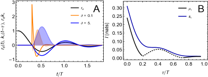
Figure 3: (A) The optimal kernel depends on the correlations and the noise $\vartheta$ in the input signal. Autocorrelation function (black) and optimal kernels $k_{*}$ at $\tau=0.3$ for oscillatory NM signals with $\eta=0.5$, for two different noise levels $\vartheta$. At low noise, the kernel consists of a positive lobe followed by a single undershoot. This corresponds to prediction based on linearly extrapolating the current signal. In contrast, at high noise, the kernel echoes the signal correlation function, exploiting signal values in the past that correlate with the future. (B) The optimal kernels $k_{*}$ strongly improve prediction over optimal exponential kernels $\mu_{*}$ (as in Fig. 2B) around $\tau=\tau_{c}\approx 0.2T$; $\vartheta=1.0$; for low noise, see Fig. S3 sup .

In contrast, oscillatory NM signals with $\eta<2$ yield optimal kernels that are oscillatory, Fig. 2D. Their shape depends on the prediction interval $\tau$, and on the correlations and noise in the input (Fig. 3A). At low noise, optimal kernels integrate only a short time window. They consist of a sharply-peaked positive lobe followed by an undershoot, effectively estimating the future signal value from its current value and derivative sup . This strategy of linear extrapolation avoids including past signals, which are inherently less correlated with the future. The capability to take derivatives enables a rapid response even when the current signal value carries no predictive information, $r_{s}(\tau)=0$; in contrast, in this situation exponential responders would need to respond slowly, to pick up past, informative signals (Fig. 2).

As noise levels $\vartheta$ rise, noise averaging becomes increasingly important, which demands longer kernels. However, to avoid signal damping, the optimal kernel must coherently sum past signal values. For oscillatory signals, this requires an oscillatory kernel, which integrates the signal with alternating signs. The prediction enhancement of globally optimal kernels over optimal exponential kernels is indeed largest for oscillatory input signals and, for $\tau\approx\tau_{c}$, it can reach up to 400% (Fig. 3B). Interestingly, in the limit $\vartheta\to\infty$, maximizing Eq. 1 gives the simple result $k_{*}(t)\propto r_{s}(t+\tau)$ sup , showing that at high noise, the optimal kernel mimics the input correlations.

Optimal oscillatory kernel shapes like $k_{*}$ in Fig. 3 can be implemented via negative feedback sup , a common motif in gene networks and signaling pathways Kondo (1997); Kholodenko (2000); Sasagawa et al. (2005). Another common motif, incoherent feedforward Alon (2006), only allows kernels with a positive lobe followed by a single undershoot sup . Our results show that this is useful for predicting low-noise non-Markovian signals, but suboptimal at high noise.

In summary, accurate prediction requires capitalizing on past signal features that are correlated with the future signal, while minimizing transmission of uncorrelated past signals and noise. Single-layer networks suffice to predict Markovian signals optimally by noise averaging. Multilayer networks predict oscillatory signals optimally, by fast linear extrapolation at low noise, and by coherent summation at high noise. In the high noise limit, the optimal network response mimics the input: $k_{*}(t)\propto r_{s}(\tau+t)$.

To explore the importance of predictive power in cellular behavior, we have studied E. coli chemotaxis. E. coli moves by alternating straight runs with tumbles, which randomly reorient it. In a spatially varying environment, this motion is biased via a signaling pathway, whose output $x(t)$ controls the propensity $\alpha(t)$ that a running bacterium will tumble. We have performed simulations of chemotaxing bacteria in static concentration fields $c(\vec{r})$ in two dimensions, using the measured response kernel $k$ Segall et al. (1986); Block et al. (1982); Celani and Vergassola (2010). At low concentrations, the signaling noise is dominated by the input noise. As in our theory, we therefore ask how the predictive power depends on the kernel and the input noise, ignoring intrinsic noise Berg (2004). The tumbling propensity is then given by $\alpha(t)=\alpha_{0}[1-x(t)]$, where $\alpha_{0}=1/\mathrm{s}$ is the basal tumbling rate and $x(t)=\int_{-\infty}^{t}k(t-t^{\prime})\ell(t^{\prime})dt^{\prime}$. The input $\ell(t^{\prime})=s(t^{\prime})+\xi(t^{\prime})$ depends on the concentration signal $s(t)=c[\vec{r}(t)]$ and the input noise $\xi(t)$ of relative strength $\theta$, arising e.g. from receptor-ligand binding or receptor conformational dynamics. The kernel $k(t)$ is adaptive, i.e. integrates to 0, which allows the bacterium to respond to a wide range of background concentrations Segall et al. (1986); Block et al. (1982). We compare adaptive kernels of varying range defined by $k_{\nu}(t)\equiv\nu^{2}k(\nu t)$, where $\nu$ defines the response speed (see also sup ).

The sensory output modulates the delay $\sim 1/\alpha(t)$ to the next tumble. This suggests that high chemotactic efficiency requires accurate signal prediction. However, it is less obvious what feature of the signal the system actually predicts: The future concentration? Or the change in concentration? More generally, what are the relevant input and output variables that control chemotaxis? Only for these variables can we expect that chemotactic performance is correlated with predictive information.

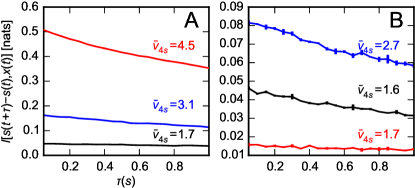
Figure 4: The predictive power of E. coli in a sinusoidal concentration field with period $L=400\mu\mathrm{m}$, generating a non-oscillatory input signal sup , as a function of the forecast interval $\tau$. Information is shown for the wild-type E. coli kernel with $\nu=1$ (blue), for a faster kernel with $\nu=3$ (red) and a slower kernel with $\nu=0.5$ (black), for noise levels $\theta=0$(A) and 2(B). Corresponding chemotactic speeds $\bar{v}_{\delta t=4\mathrm{s}}$ are given in $\mu\mathrm{m}/\mathrm{s}$. Bacteria run at $20\mu\mathrm{m}/\mathrm{s}$.

To address this question, we performed simulations for three different kernels, $\nu=0.5,1,3$ where $\nu=1$ corresponds to the measured kernel, and for two input noise levels, $\theta=0,2$. As our performance measure, we use the mean chemotactic speed $\bar{v}_{\delta t}=\bigl{\langle}\frac{[\vec{r}(t+\delta t)-\vec{r}(t)]\cdot\nabla c[\vec{r}(t)]}{\delta t\|\nabla c[\vec{r}(t)]\|}\bigr{\rangle}$; similar results are obtained for the mean concentration $\langle{}c[\vec{r}(t)]\rangle$ sup . We find that $\bar{v}_{\delta t}$ is poorly correlated with the predictive information $I[x,s_{\tau}]$ between current output and future concentration sup . In contrast, it is well correlated with the predictive information $I[x,s_{\tau}-s]$ between current output and future concentration change, as Fig. 4 shows. Hence, the search strategy of E. coli is not based on predicting the future concentration, but rather its trend, in accordance with the observation that the bilobed kernel $k$ takes a time-derivative of the signal. If this is positive, E. coli ‘expects’ that the concentration will continue to rise, and will extend its run.

Fig. 4 also shows that the optimal kernel that maximizes the information and hence chemotactic speed, depends on the input noise $\theta$. A fast kernel emphasizes up-to-date information about recent concentration changes, enabling an accurate and rapid response at low noise. At high noise, its performance drops because it cannot filter the input noise and hence cannot reliably predict future concentration changes. The optimal kernel range then arises from a trade-off between agility and robustness.

Lastly, how far must E. coli look into the future for efficient chemotaxis? To anticipate concentration changes, the prediction horizon, i.e. the time over which predictive information extends, should exceed the response time. According to Eq. 1 the prediction horizon is bounded by the signal correlation time, which is determined by the length scale of the concentration field and by the motile behavior, to be explored in future work. Already, Fig. 4 indicates that the prediction horizon of E. coli is indeed longer than the response time, as $I(\tau)$ decays slower than $1/\alpha_{0}=1\mathrm{s}$. Our results thus suggest that E. coli can indeed reliably anticipate concentration changes.

We thank Thomas Ouldridge, Tom Shimizu, and Giulia Malaguti for stimulating discussions and a critical reading of the manuscript. This work is part of the research program of the “Stichting FOM”, which is financially supported by the “Nederlandse organisatie voor Wetenschappelijk Onderzoek” (NWO). NBB was supported by a fellowship of the Heidelberg Center for Modeling and Simulation in the Biosciences (BIOMS).

Appendix A Supplementary Material

A.1 Predictive information limits fitness when cells adapt with a delay

The predictive mutual information between input and output is a biologically relevant measure Taylor et al. (2007); Bialek (2012); Bergstrom and Lachmann (2005) for the performance of the system. Imagine a cell which instantaneously senses a slowly varying nutrient concentration $s$, with intracellular output $x$, and as a result, grows at a rate $g(x,s)$ that is maximal for some optimally adapted value of $x(s)$. In this setting, it was shown Taylor et al. (2007) that the instantaneous mutual information $I[x,s]$ sets an upper limit for the achievable growth rate.

Now imagine that the cell’s adaptive response (e.g, enzyme production) requires finite time $\tau$ to mount. Since only available enzymes can process nutrients, the growth rate lags behind the output $x$, as $g(t+\tau)=g[x(t),s(t+\tau)]$. Repeating the argument of Taylor et al. (2007), the predictive information $I[x,s_{\tau}]=I[x(t),s(t+\tau)]$ now limits the achievable growth rate. This makes maximizing $I[x,s_{\tau}]$ a plausible design goal for dynamic sensory networks.

We have considered a fixed delay time $\tau$ for simplicity, leading to the mutual information $I[x,s_{\tau}]$ as a relevant information measure, which is distinct from both the predictive information between entire past and future trajectories Bialek et al. (2001) and the information rate between input and output trajectories Tostevin and ten Wolde (2009). Distributed delays for the adaptive cellular response of the cell would correspond to yet different predictive information definitions in which future time points are weighted according to a delay distribution; such refinements are left for future work.

A.2 Instantaneous response is optimal for noiseless Markovian signals

Consider first a general input signal, Markovian or not. Denote the full signal history up to but excluding $t$ by $[s]$, the present signal by $s=s(t)$, the present output by $x=x(t)$, and a future signal by $s_{\tau}=s(t+\tau)$, respectively. We require that the output does not feed back onto the signal. This implies that future signal values are independent of the response for given signal history: $p(s_{\tau}|x,[s],s,t)=p(s_{\tau}|[s],s,t)$.

We can then expand the predictive two-point distribution $p(s_{\tau},x|s,t)$ over the driving history:

$$p(s_{\tau},x|s,t)=\int\mathcal{D}[s]p(s_{\tau},x,[s]|s,t)$$

$$=\int\mathcal{D}[s]p(s_{\tau}|x,[s],s,t)p(x|[s],s,t)p([s]|s,t)$$

$$=\int\mathcal{D}[s]p(s_{\tau}|[s],s,t)p(x|[s],s,t)p([s]|s,t),$$ (S1)

where the second equality uses the basic rule $p(x,y|z)=p(x|y,z)p(y|z)$, and the last equality uses the absence of feedback.

If the response is instantaneous, we have the relation $p(x|[s],s,t)=p(x|s,t)$; if the input is Markovian, $p(s_{\tau}|[s],s,t)=p(s_{\tau}|s,t)$. In either case we can integrate Eq. A.2 over $[s]$ and obtain

$$p(s_{\tau},x|s,t)=p(x|s,t)p(s_{\tau}|s,t).$$ (S2)

So, if the input $s$ is Markovian, history-dependent and instantaneous responders behave the same: $s_{\tau}$ and $x$ are independent when conditioned on $s$. In other words, the variables $x\leftrightarrow s\leftrightarrow s_{\tau}$ form a Markov chain Cover and Thomas (2012). They therefore obey the data processing inequality $I[x,s_{\tau}]\leq I[s,s_{\tau}]$.

This implies that predictions based on measuring $x$ cannot surpass those based on the current input $s$, even if $x$ depends on the history $[s]$ in arbitrarily complicated ways. Thus, an instantaneous responder for which $x$ faithfully tracks the current input $s$, can already achieve the maximal performance $I[s,s_{\tau}]$. Note that this requires $s$ to be noiseless; in contrast, degraded Markovian signals can be better predicted with memory, as discussed in the main text.

A.3 Optimal prediction of Gaussian signals
by linear networks

In this section we consider optimal linear prediction strategies for input concentration signals that are stationary Gaussian processes. An input signal $s(t)$ is presented to the responder in form of a ligand number $\ell(t)$ subject to molecular noise. Ligands are sensed by a sensory network which operates in a linear regime but is otherwise arbitrary, possibly including multiple stages and feedback loops. We impose the restriction that the network does not have any influence on the input, for instance, by sequestering ligands and thereby reducing the current available ligand number. Since we are interested in how the accuracy of prediction depends on the noise and the correlations in the input signal, we focus on responders in the deterministic limit.

In this linear regime, we can expand the input $s(t)$ and degraded input $\ell(t)$ around their steady state values, and subtract the latter, so that in the following $\langle{}s\rangle=0$ and $\langle{}\ell\rangle=0$ without restriction. The degraded input is modeled as

$$\ell(t)=s+\xi,$$ (S3)

where $\xi$ is independent, Gaussian white noise with $\langle{}\xi(t)\xi(t^{\prime})\rangle=\sigma_{s}^{2}\vartheta^{2}\delta(t-t^{\prime})$ and $\sigma_{s}$ denotes the standard deviation of the pure, non-noisy input process. The white noise $\xi$ approximates a physical noise process $n$ with variance $\sigma_{n}^{2}$ and finite but short correlation time $\tau_{n}$. Its effect on the final output of the signaling network is determined by the integrated strength $\int_{0}^{\infty}\langle{}n(0)n(t)\rangle dt=\sigma_{n}^{2}\tau_{n}$. The integrated strength of $\xi$ is $\sigma_{s}^{2}\vartheta^{2}$. Thus, $\vartheta^{2}$ measures the integrated noise strength relative to the signal variance, and has units of time.

Since we disregard responder noise, the absolute amplitude of the signal $\sigma_{s}$ is irrelevant, as will be clarified shortly. The sensory output is then given as a convolution

$$x(t)=\int_{-\infty}^{t}\ell(t^{\prime\prime})k(t-t^{\prime\prime})dt^{\prime\prime}=\int_{0}^{\infty}\ell(t-t^{\prime\prime})k(t^{\prime\prime})dt^{\prime\prime},$$ (S4)

where memory of past signal values is encoded by the linear response kernel $k$. The output $x$ is correlated with the input. Here and in the following, we use $c_{xy}=\langle{}xy\rangle$ and $r_{xy}=c_{xy}/\sigma_{x}\sigma_{y}$ to denote covariance functions and correlation functions, respectively, and abbreviate $r_{xx}=r_{x},c_{xx}=c_{x}$. Then the predictive input-output correlation is given by

$$r_{xs}(\tau) =r_{xs_{\tau}}=\frac{c_{xs_{\tau}}}{\sigma_{x}\sigma_{s}}$$

$$=\frac{\int_{0}^{\infty}\langle{}[s(t^{\prime}-t^{\prime\prime})+\xi(t^{\prime}-t^{\prime\prime})]k(t^{\prime\prime})s(t^{\prime}+\tau)\rangle dt^{\prime\prime}}{\sigma_{x}\sigma_{s}}$$

$$=\frac{\int_{0}^{\infty}r_{s}(t^{\prime}+\tau)k(t^{\prime})dt^{\prime}}{\sigma_{x}/\sigma_{s}}$$

$$=\frac{\int_{0}^{\infty}r_{s}(t^{\prime}+\tau)k(t^{\prime})dt^{\prime}}{\bigl{[}\int_{0}^{\infty}k(t)[r_{s}(t-t^{\prime})+\vartheta^{2}\delta(t-t^{\prime})]k(t^{\prime})dtdt^{\prime}\bigr{]}^{1/2}}.$$

$$\equiv\frac{\Psi}{[\Sigma+\Xi]^{1/2}}$$ (S5)

Importantly, since $s$ and $x$ are jointly Gaussian, the predictive information evaluates to $I[x,s_{\tau}]=-\log[1-r_{xs}(\tau)^{2}]/2$, a simple function of the cross-correlation, see also Tostevin and ten Wolde (2009, 2010). Since $r_{xs}$ does not depend on the absolute signal amplitude $\sigma_{s}$, neither does the predictive information. The numerator of the last equation defines the overlap integral between the current output $x(t)$ and the future input $s(t+\tau)$, normalized by the input variance $\sigma^{2}_{s}$: $\Psi\equiv c_{xs_{\tau}}/\sigma^{2}_{s}=\int_{0}^{\infty}r_{s}(t^{\prime}+\tau)k(t^{\prime})dt^{\prime}$. The denominator defines the part of the normalized output variance $\sigma^{2}_{x}/\sigma^{2}_{s}$ that is due to the past input signal $s(t)$, $\Sigma\equiv\int_{0}^{\infty}k(t)r_{s}(t-t^{\prime})k(t^{\prime})dtdt^{\prime}$, and the part which is due to past noise $\xi(t)$, $\Xi\equiv\vartheta^{2}\int_{0}^{\infty}k(t)^{2}dt$.

A.4 Exponential response kernels

In this section, we consider systems with exponential response kernels. The input signals are either Markovian or non-Markovian, with the latter being generated from the harmonic-oscillator model as described in the main text.

A.4.1 Optimal response speeds

We can readily evaluate $r_{xs}(\tau)$ for systems with exponential response kernels, $k\propto\exp(-\mu t)$. For Markovian (M) Ornstein-Uhlenbeck signals with $r_{s}(t)=\exp(-\lambda t)$ we obtain

$$r_{xs}^{\text{M}}(\tau)=\exp(-\lambda\tau)\bigl{[}(\mu+\lambda)(1+\vartheta^{2}(\mu+\lambda)/2)/\mu\bigr{]}^{-1/2}.$$ (S6)

Maximizing the correlation yields the optimal response speed $\mu_{\text{ti}}=(2\lambda/\vartheta^{2}+\lambda^{2})^{1/2}$.

For a NM signal with damping coefficient $\eta$, the correlation coefficient, after some algebra, results as

$$r_{xs}^{\text{NM}}(\tau)=\hskip 140.00021pt$$ (S7)

$$\frac{e^{-\frac{1}{2}\tau\eta_{+}}[2-2\eta_{-}(\eta+\mu)]-e^{-\frac{1}{2}\tau\eta_{-}}[2-2\eta_{+}(\eta+\mu)]}{(\eta\mu+\mu^{2}+1)\bar{\eta}\bigl{[}\frac{8}{a_{+}}+\frac{8}{a_{-}}+\frac{-2\eta^{2}\vartheta^{2}\mu^{2}+4\eta+2\vartheta^{2}\left(\mu^{2}+1\right)^{2}}{-\left(\eta^{2}-2\right)\mu^{3}+\mu^{5}+\mu}\bigr{]}^{1/2}},$$

where

$$a_{\pm} =\sqrt{\eta\eta_{\pm}-1}[\eta^{2}\eta_{\pm}+2(\mu^{2}+1)\bar{\eta}-4\eta]\text{, }$$

$$\eta_{\pm} =\tfrac{1}{2}(\eta\pm\bar{\eta})\text{, and }\bar{\eta}=\sqrt{\eta^{2}-4}.$$

Maximization of $(r_{xs}^{\text{NM}})^{2}$ with respect to the response speed $\mu$ can be done numerically and yields a characteristic discontinuity at finite $\tau$; see Fig. 2B of the main text.

The resulting predictive informations $I$ are plotted in Fig. 1 of the main text for signals with moderate intrinsic stochasticity $\eta>0.5$. For comparison, Fig. S1 shows the predictive information achieved for long-range correlated non-Markovian (NM) harmonic oscillator signal at $\eta=10^{-4}$. Without noise and for prediction interval $\tau>0.2$, a slow response can induce a delay $\Lambda$ that leads to optimal anticorrelation with the future signal, by achieving anti-phase matching $\Lambda+\tau=T/2$ (peaks in Fig. S1). In fact, when taking $\eta\to 0$, the mutual information between these two perfectly anticorrelated time points diverges. Input noise (dashed lines) regularizes the divergence, leaving pronounced maxima at the delays that produce the best (anti)phase matching.

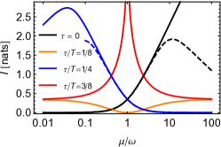
Figure S1: Predictive information of exponential responders for highly correlated NM signals with $\eta=10^{-4}$. Noise strength $\vartheta=0,0.05$, solid and dashed lines, respectively. Cf. also Fig. 2D

A.4.2 Scaling argument: Time integration leads to an optimal response speed $\mu_{\text{ti}}$ for noisy signals

We consider the scaling of Eq. 1 (or Eq. S5) with the effective integration time $t_{\text{int}}$ in a simplified setting. Let $r_{s}$ and $k$ be positive, monotonically decreasing and of finite support. Specifically, let $k(0)=1$, and $k(t)=0$ for $t>t_{\text{int}}$, the integration time, and let $r_{s}(t)=0$ for $|t|>t_{s}$, the correlation time.

Then, in the regime $t_{\text{int}}<t_{s}-\tau$, the overlap $\Psi(\tau)=\int_{0}^{\infty}r_{s}(t+\tau)k(t)dt$ in the numerator of Eq. 1 increases roughly linearly with increasing $t_{\text{int}}$. In the denominator, the contribution of past signals to the output variance $\Sigma=\int kr_{s}k\propto t_{\text{int}}^{2}$ while the noise contribution $\Xi=\vartheta^{2}\int k^{2}\propto t_{\text{int}}$. Thus for short integration times, the noise contribution dominates and $r_{xs_{\tau}}^{2}$ increases $\propto t_{\text{int}}/\vartheta^{2}$ due to noise averaging. This initial scaling regime exists only for noisy signals $\vartheta>0$; it is the reason why short-time integration benefits predictions.

When the integration time exceeds the signal correlation time, a new regime appears where the overlap integral $\Psi$ saturates to a constant, but both $\Sigma\propto t_{\text{int}}$ and $\Xi\propto t_{\text{int}}$ continue to grow, so that $r_{xs_{\tau}}^{2}\propto t_{\text{int}}^{-1}$. This decrease in predictive power at long integration times reflects the fact that very long signal integration confounds predictions by including uncorrelated past signals; this scaling regime therefore exists with or without noise. In effect, uncorrelated, past signal values are a source of noise, which hampers prediction.

We conclude that in the presence of noise, there exists an optimal response speed $1/t_{\text{int}}^{\vartheta}<\mu_{\text{ti}}<1/t_{s}$ that allows noise averaging but excludes confounding past signals.

In the above analysis, we have modeled the noise as white Gaussian noise. The same arguments still apply when the correlation time of the noise is finite, but shorter than the signal correlation time. In that case, there also exists an optimal response time that arises from the trade-off between noise averaging and excluding past signal values uncorrelated with the future. The situation is different in the opposite limiting case where the noise correlation time is longer than that of the signal. Here we expect that an adaptive filter may be beneficial for predicting the future; we leave this for future work.

A.4.3 Exploitation of non-monotonic signal autocorrelations yields an optimal response speed $\mu_{*}$

Non-exponential autocorrelations can generate an optimal response speed $\mu_{*}$ even without noise. Without noise, $t_{\text{int}}^{\vartheta}=0$, and the arguments in the previous section do not allow the conclusion that there is an upper bound for the optimal response speed. In fact, we know already that when the input signal is Markovian, an instantaneous response is optimal.

However, when the input signal is non-Markovian, there exists a finite response speed even in the absence of noise in the input. One way to see this is to consider only exponential responders $k(t)=\exp(-\mu t)$ and expand for high speeds $\mu$. One obtains

$$r_{xs_{\tau}}^{2}=r_{s}(\tau)^{2}\bigl{[}1+\tfrac{2}{\mu}\bigl{(}\tfrac{r_{s}^{\prime}(\tau)}{r_{s}(\tau)}-\tfrac{r_{s}^{\prime}(0)}{r_{s}(0)}\bigr{)}\bigr{]}+O(\mu^{-2}).$$ (S8)

One sees that in the case of exponential $r_{s}$, the sub-leading $1/\mu$-term vanishes exactly; this is compatible with the fact that the optimal response for Markovian noiseless signals is instantaneous, as discussed above. In contrast, when the autocorrelation function $r_{s}(t)$ of the input signal is non-monotonic or becomes negative, lagging responders with finite $\mu$ can make the $1/\mu$ term positive and thus improve predictions over the instantaneous response $\mu\to\infty$. This shows that instantaneous responders are not globally optimal predictors at least for some non-Markovian noiseless signals.

Fig. S2 gives an intuitive explanation of the mechanism of exploitation of correlated past signals. In essence, a lagging kernel weights heavily the past signal values $s(t^{\prime})$ at those time points that are strongly correlated with the prediction target $s(t+\tau)$, as reported by the shifted autocorrelation $r_{s}(t+\tau)$.

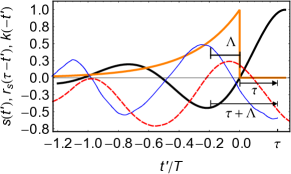
Figure S2: Exploiting signal correlations to predict the future. For the linear networks studied here, the output $x(t)$ (dashed, red) at time $t=0$ is given by $x(0)=\int_{-\infty}^{0}k(-t^{\prime})s(t^{\prime})$. Hence, the kernel $k(-t^{\prime})$ (orange) integrates the signal $s(t^{\prime})$ (blue) over past time points $t^{\prime}<0$. The challenge is to pick up the signals $s(t^{\prime})$ from the past that are most correlated with the future signal $s(\tau)$ that is to be predicted. An instantaneous kernel would include signals around $t^{\prime}=0$ which contain little information about $s(\tau)$, as can be seen from the zero-crossing of the signal autocorrelation function $r_{s}(\tau-t^{\prime})$ (black) at $t^{\prime}=0$. In contrast, the lagging kernel $k=k_{*}$, shown in orange, emphasizes the negative lobe of $r_{s}$, picking up signal values from the past that are strongly anticorrelated with the future signal $s(\tau)$. This maximizes predictive power. Effectively, this kernel generates a response $x(t)$ that lags behind the input $s(t)$ with a lag $\Lambda$, so that the current output $x(0)$ reflects the past input $s(-\Lambda)$ rather than the current input $s(0)$. The optimal lag obeys $\tau+\Lambda\simeq T/2$, with $T$ the period of the signal oscillation: $r_{s}(\Lambda+\tau)$ is, indeed, strongly negative. In this example, $\eta=0.5$, so that the signal $s(t)$ is oscillatory.

In particular, when $r_{s}(t)$ is non-monotonic, the overlap $\Psi(\tau)$ and the signal-induced variance $\Sigma$ depend strongly on the shape of the kernel and autocorrelation functions. $r_{xs_{\tau}}^{2}$, and $I$, is maximized when the kernel overlaps well with the back-shifted autocorrelation, increasing $\Psi(\tau)^{2}$, while overlapping weakly with forward-shifted autocorrelations, decreasing $\Sigma=\int\Psi(-t^{\prime})k(t^{\prime})dt^{\prime}$. Thus, an optimal kernel selects past signals that are correlated with the future signal while rejecting confounding past signals. This basic strategy continues to be effective at finite noise levels, where noise averaging and exploitation of correlations are combined via Eq. 1, as seen in Fig. 1D.

A.5 Wiener-Kolmogorov filtering theory for predicting biochemical signals

We are interested in finding a response kernel with optimal predictive power. In signal processing, statistically optimal filters are well known; in particular, the Wiener filter Kolmogorov (1992); Wiener (1950) is the linear response kernel $k_{*}$ that minimizes the mean squared error between a general output $o$ and input $i$, $e_{io}=\langle{}(i-o)^{2}\rangle=\min$. This criterion is different from optimal predictive power, $I[i,o]=\max$. However, in the case of Gaussian signals, both are closely related.

For Gaussian signals, the Wiener filter is optimally informative

In order to minimize the mean squared error

$$e_{io}=\sigma_{i}^{2}+\sigma_{o}^{2}-2\sigma_{i}\sigma_{o}r_{io}.$$ (S9)

for given input statistics, we are free to start by rescaling the output variable (by adjusting the kernel amplitude). The optimal scale is attained when $de_{io}/d{\sigma_{o}}=0$, or $\sigma_{o}=\sigma_{i}r_{io}$ (recall that $r_{io}$ does not depend on the output scale). The latter equation makes sense only if $r_{io}>0$; we can ensure this by inverting the kernel if necessary. Inserting this result, $e_{io}=\sigma_{i}^{2}(1-r_{io}^{2})$. Since the input amplitude is fixed, we conclude that $e_{io}=\min\Rightarrow r_{io}^{2}=\max$. Conversely, for Gaussian signals, $I=\max\Leftrightarrow r_{io}^{2}=\max$. Together, this shows that the predictive information is maximized by any kernel in the family $\{\alpha k_{*}\}_{\alpha\neq 0}$, which maximally correlate ($\alpha>0$) or anticorrelate ($\alpha<0$) with the input. We can thus exploit the Wiener-Kolmogorov filter theory to construct optimally informative response functions for Gaussian signals.

Construction of the Wiener-Kolmogorov causal filter

The causal Wiener filter is the optimally predictive kernel $k_{*}$ which depends only on past signal values. We briefly recall the construction of $k_{*}$ for given signal correlations, noise levels and prediction interval. Let the Fourier transform of the degraded input autocovariance, $c_{\ell}(\omega)\equiv\mathcal{F}[c_{\ell}](\omega)=\int_{-\infty}^{\infty}c_{\ell}(t)e^{-i\omega t}dt$. Define the causal part of a function $f(\omega)$ as $[f]_{+}(\omega)=\mathcal{F}[\theta\mathcal{F}^{-1}[f]](\omega)$ where $\theta$ is multiplication with the unit step function. Now, find a Wiener-Hopf factorization $c_{\ell}(\omega)=m_{+}m_{-}$, which is defined by the properties $m_{-}(\omega)=m_{+}(\omega)^{*}=m_{+}(-\omega)$ which ensure that $m_{\pm}$ are real functions in the time domain; and by the requirement that $m_{+}$ and $1/m_{+}$ be causal, that is, their inverse transforms vanish for all $t<0$, which can be written as $m_{+}=[m_{+}]_{+}$ and $1/m_{+}=[1/m_{+}]_{+}$, respectively. Then the causal Wiener filter is given by Wiener (1950)

$$k_{*}(\omega)=\frac{1}{m_{+}(\omega)}\Bigl{[}\frac{c_{\ell s_{\tau}}(\omega)}{m_{-}(\omega)}\Bigr{]}_{+}.$$ (S10)

This general result simplifies in our case of independent white noise, Eq. S3. Here, $c_{\ell}(t)=\sigma_{s}^{2}[r_{s}(t)+\vartheta^{2}\delta(t)]$, so that $c_{\ell s}(\omega)=c_{s}(\omega)=c_{\ell}(\omega)-\sigma_{s}^{2}\vartheta^{2}$. Noting that the predictive cross-covariance satisfies $c_{\ell s_{\tau}}(\omega)=c_{\ell s}(\omega)e^{i\omega\tau}$, we obtain

$$k_{*}=\frac{1}{m_{+}}\Bigl{[}\Bigl{(}m_{+}-\frac{\sigma_{s}^{2}\vartheta^{2}}{m_{-}}\Bigr{)}e^{i\omega\tau}\Bigr{]}_{+}=m_{+}^{-1}\bigl{[}m_{+}e^{i\omega\tau}\bigr{]}_{+},$$ (S11)

where we substituted the factorization of $c_{\ell}$ and in the last equality, used the fact that $1/m_{-}$ and even more so, the back-shifted $e^{i\omega\tau}/m_{-}$, has no causal part.

When is the instantaneous response optimally predictive?

With this general expression we can answer the question under what conditions the instantaneous response is optimal. According to Eq. S11, this happens exactly when $k_{*}(\omega)=m_{+}^{-1}\bigl{[}m_{+}e^{i\omega\tau}\bigr{]}_{+}=a$ is a real constant, since then $k_{*}(t)\propto\delta(t)$. This occurs if and only if $m_{+}(t+\tau)/m_{+}(t)=a$ for all $t\geq 0$. By writing $c_{\ell}(t)=\int m_{+}(t^{\prime})m_{-}(t-t^{\prime})dt^{\prime}$, this can be seen to imply

$$c_{\ell}(t+\tau)=ac_{\ell}(t),\,t\geq 0,$$ (S12)

where a bounded signal requires $|a|\leq 1$. We conclude that the input correlation $c_{\ell}(t)$ must decay exponentially, possibly modulated by oscillations; in the latter case, the forecast interval $\tau$ must be a multiple of the period.

This condition is quite restrictive. First, Eq. S12 pertains to the degraded input $c_{\ell}$, not the signal $c_{s}$ itself. This means that an instantaneous responder cannot be optimal when there is noise in the input signal, since if $\vartheta>0$, $c_{\ell}(t)$ would exhibit a $\delta$-peak at $t=0$, violating Eq. S12. This observation agrees also with the scaling analysis above which found that for noisy input, short-time integration is beneficial. Second, if the input decays with exponentially damped oscillations, then Eq. S12 requires that the prediction interval is a multiple of the input period. This requirement corresponds to predicting only exactly phase-related future time points via a simple phase matching mechanism.

We conclude that an instantaneous, $\delta$-shaped responder is optimal only in the contrived limit in which (a) the input is noiseless; and (b) the input decays exponentially (the Markovian signal), or it decays with exponentially damped oscillations and the forecast interval $\tau$ is a multiple of the input period $T$.

A.6 Computation of optimal kernels

We now give explicit expressions for optimally predictive kernels for several input signal types.

A.6.1 Optimal kernels for Markovian signals

The Markovian (M) signal autocorrelation reads $r_{s}(t)=\exp(-\lambda|t|)$ for some positive damping coefficient $\lambda$. The power spectral density of the degraded input is $c_{\ell}(\omega)=\frac{2\lambda}{\lambda^{2}+\omega^{2}}+\vartheta^{2}$, for which we find a Wiener-Hopf factorization

$$m_{\pm}(\omega)=\frac{\zeta\pm i\vartheta\omega}{\lambda\pm i\omega};\;\zeta=\sqrt{2\lambda+\lambda^{2}\vartheta^{2}}$$ (S13)

and finally the result

$$k_{*}^{\text{M}}(\omega)=e^{-\lambda\tau}\frac{\zeta-\lambda\vartheta}{\zeta+i\vartheta\omega}.$$ (S14)

In the noiseless limit $\vartheta\to 0$, the kernel reduces to a constant $e^{-\lambda\tau}$ in the frequency domain, confirming that indeed for noiseless Markovian signals, an instantaneous responder has optimal predictive power. (Note that this is compatible with Eq. S12.) For positive noise strength $\vartheta>0$, the optimal kernel in the time domain reads

$$k_{*}^{\text{M}}(t)\propto\theta(t)e^{-\mu_{\text{ti}}t}\text{, where }\mu_{\text{ti}}=\sqrt{\lambda^{2}+2\lambda/\vartheta^{2}}.$$ (S15)

That is, the input noise is filtered optimally by an exponential moving average; the averaging time constant $1/\mu_{\text{ti}}$ arises from time integration, since the Markovian signal does not provide extra information in past signal values. The time constant increases from 0 for weak noise towards $1/\lambda$, the input signal correlation time, for strong noise. $\mu_{\text{ti}}$ (necessarily) agrees with the optimal response speed found previously, when optimization was restricted to exponential responders only. Thus, a lagging response improves prediction of noisy Markovian signals, by allowing a better estimate of the current signal value $s(t)$ through averaging; this is the best strategy possible with a linear responder.

A.6.2 Optimal kernels for noiseless non-Markovian signals

In the NM case, defined as in the main text by the Langevin equations $\partial_{\omega t}q=p,\;\partial_{\omega t}p=-q-\eta p+\sqrt{2\eta}\psi$, we set $q\equiv s$. Note that the process $(q(t),p(t))$ is indeed a Gaussian process; this follows from the fact that future signals are generated as a linear combination of present signals and Gaussian noise, and that Gaussian random variables are stable under linear combination. Since the Langevin equations do not depend on time explicitly, after some transient period, the process is stationary.

The power spectral density of the degraded input becomes

$$c_{\ell}(\omega)=\frac{2\eta}{\omega^{4}+(\eta^{2}-2)\omega^{2}+1}+\vartheta^{2}.$$ (S16)

Considering first the case without input noise $\vartheta=0$, we exploit the fact that $m_{+}$ is proportional to the dynamic susceptibility of the harmonic oscillator, to obtain $m_{+}(\omega)\propto(\omega^{2}-i\eta\omega-1)^{-1}$, or in the time domain, $m_{+}(t)\propto\theta(t)e^{-\eta t/2}\sin(\eta^{\prime}t/2)/\eta^{\prime}$, where $\eta^{\prime}=\sqrt{4-\eta^{2}}$. One then obtains the optimal response

$$k_{*}^{\text{NM}}\propto\bigl{(}\cos\tfrac{\eta^{\prime}\tau}{2}+\tfrac{\eta}{\eta^{\prime}}\sin\tfrac{\eta^{\prime}\tau}{2}\bigr{)}\delta(t)+\bigl{(}\tfrac{2}{\eta^{\prime}}\sin\tfrac{\eta^{\prime}\tau}{2}\bigr{)}\dot{\delta}(t).$$ (S17)

Recalling that by definition,

$$\int[a(\tau)\delta(t)-b(\tau)\dot{\delta}(t)]\ell(t-t^{\prime})dt^{\prime}=a(\tau)\ell(t)+b(\tau)\dot{\ell}(t),$$

one sees that this response kernel implements prediction by linear extrapolation. The network output is a linear combination of the current signal value $\ell(t)$ and derivative $\dot{\ell}(t)$ whose coefficients $a(\tau)$ and $b(\tau)$ depend on the signal statistics and prediction interval $\tau$. This singular kernel can be thought of as the limit of a kernel with a sharp positive peak at $t\to 0$ immediately followed by a single sharp underswing; such a kernel yields an output which effectively is a weighted sum of the current input signal value and its derivative, the weights of which are determined by the positive and negative lobe of the kernel. Although the noiseless case is an oversimplified singular limit, the low-noise regime can be understood in similar terms, see below and the low-noise kernel in Fig. 3A.

As a special case, notice that in the underdamped regime $\eta<2$, $\eta^{\prime}$ is real. When the prediction interval $\tau$ is chosen as a multiple of the signal period $2\pi/\eta^{\prime}$, the $\delta^{\prime}$ term in Eq. S17 vanishes. Then, the optimal response strategy reduces to instantaneous readout of the signal. This finding reproduces the previous general result Eq. S12.

A.6.3 Optimal kernels for non-Markovian signals with noise

In the general NM case including input noise $\vartheta>0$, we may expect that as for the Markovian signal, noise suppression through averaging becomes relevant. We write Eq. S16 as a single fraction and factorize the numerator into causal and anticausal parts. Combined with the noiseless result, this yields

$$m_{+}\propto\frac{\vartheta\omega^{2}-i\zeta_{2}^{+}\omega-\zeta_{1}}{\omega^{2}-i\eta\omega-1},$$ (S18)

where we define $\zeta_{1}=(2\eta+\vartheta^{2})^{1/2}$ and $\zeta_{2}^{\pm}=(\vartheta[(\eta^{2}-2)\vartheta\pm 2\zeta_{1}])^{1/2}$. With some algebra, the optimal kernel in the Fourier domain can be written as

$$k_{*}^{\text{NM}}\propto\bigl{[}\vartheta\omega^{2}-i\zeta_{2}^{+}\omega-\zeta_{1}\bigr{]}^{-1}\times\\ \Bigl{\{}-i\omega(\eta-\zeta_{2}^{+}/\vartheta)\bigl{[}\tfrac{\zeta_{2}^{+}}{\eta^{\prime}}\sin\tfrac{\tau\eta^{\prime}}{2}+\vartheta\cos\tfrac{\tau\eta^{\prime}}{2}\bigr{]}+\\ +\tfrac{\eta\left(\vartheta+\sigma_{1}\right)-2\zeta_{2}^{+}}{\eta^{\prime}}\sin\tfrac{\tau\eta^{\prime}}{2}+(\zeta_{1}-\vartheta)\cos\tfrac{\tau\eta^{\prime}}{2}\Bigr{\}}.$$ (S19)

The corresponding time-domain kernel is a superposition of exponential terms with prefactors depending on signal, noise and the prediction interval; and ‘rate constants’ $\mu_{*}^{\pm}=(\zeta_{2}^{+}\pm\zeta_{2}^{-})/(2\vartheta)$ determined by the poles in the complex $\omega$-plane of Eq. S19, independent of the prediction interval $\tau$.

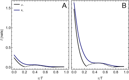
Figure S3: (A) Predictive information $I[x,s_{\tau}]$ for NM signals at $\eta=0.5,\vartheta=1$ for optimal exponential kernels $\mu^{*}=\mu^{*}(\tau)$ (black; dashed region indicates $xs_{\tau}$ anticorrelation as in Fig. 2B); and for the respective globally optimal kernel $k_{*}$, which is non-monotonic (top blue line). (B) as (A) but a low noise $\vartheta=0.1$. Note that (A) is the same as Fig. 3B in the main text.

The optimal exponential kernel with $\mu=\mu_{*}(\tau)$ improves performance as a function of $\tau$ over any fixed exponential kernel; however, it still suffers from the poor correspondence of signal and kernel shape when $\tau\simeq\tau_{c}$, where the correlation function is close to a zero-crossing and the exponential response switches between correlated and anticorrelated output, Fig. S3A. The optimal, non-monotonic, kernel $k_{*}$ improves predictions strongly over even the best-adapted exponential kernel, Fig. S3A, in particular around the critical prediction interval $\tau_{c}$, where an oscillatory kernel can exploit signals on both sides of the zero-crossing of $r_{s}$, avoiding precision loss due to cancellations. At low noise, performance is better in general, Fig. S3B, but the advantage of the optimal kernel over exponential kernels persists.

A.6.4 General expression for optimal kernels at high noise

In the Markovian case, we have seen that as the noise strength $\vartheta$ diverges, the optimal kernel becomes proportional to the signal autocorrelation function. This is in fact a general result which applies to arbitrary Gaussian input signals. We recall that for white noise, $c_{\ell}(\omega)=c_{s}(\omega)+\vartheta^{2}\sigma_{s}^{2}$, and expand the factors $m_{\pm}$ as $m_{\pm}=\vartheta m_{\pm}^{0}+\vartheta^{-1}m_{\pm}^{1}+O(\vartheta^{-3})$, so that comparing $c_{\ell}=m_{+}m_{-}$ order by order gives $\sigma_{s}^{2}=m_{+}^{0}m_{-}^{0}$ and $c_{s}=m_{+}^{0}m_{-}^{1}+m_{-}^{0}m_{+}^{1}$. Since $\sigma_{s}$ is a real constant, this implies $m_{\pm}^{0}=\sigma_{s}$, and $m_{+}^{1}=c_{s}/\sigma_{s}-m_{-}^{1}$.

Now recall that the kernel is given by Eq. S11,

$$k_{*}(\omega)=\frac{\bigl{[}(\sigma_{s}+\vartheta^{-2}m_{+}^{1})e^{i\omega\tau}\bigr{]}_{+}}{\sigma_{s}+\vartheta^{-2}m_{+}^{1}}=\frac{\vartheta^{-2}\bigl{[}(c_{s}/\sigma_{s})e^{i\omega\tau}\bigr{]}_{+}}{\sigma_{s}+\vartheta^{-2}m_{+}^{1}},$$ (S20)

where the second equality follows after substituting $m_{+}^{1}$ and eliminating all anticausal terms in the causal bracket. The last expression, to leading order gives just $\vartheta^{2}k_{*}=[c_{s}e^{i\omega\tau}]_{+}$. This proves that the optimal kernel, to leading order for high noise, is proportional to the signal autocorrelation function, back-shifted by the prediction interval $\tau$, or $k_{*}(t)\propto\theta(t)c_{s}(t+\tau)$. We note that the same result can also be obtained by functionally maximizing the predictive correlation $r_{xs_{\tau}}$ with respect to the kernel in the high noise limit.

A.7 Networks that implement optimal kernels for oscillatory signals

The optimal kernel Eq. S19 for the noisy NM signal has a complicated dependence on the parameters, but a simple time dependence $k_{*}(t)\propto a^{+}e^{-\mu_{*}^{+}t}+a^{-}e^{-\mu_{*}^{-}t}$. In the interesting underdamped regime, $\mu^{*\pm}=\mu_{*}\pm i\omega_{*}$ are complex conjugates with positive real part, so that $k(t)\propto e^{-\mu_{*}t}[a\sin(\omega_{*}t)+b\cos(\omega_{*}t)]$. Can such a damped oscillatory optimal kernel be implemented with a simple two-stage biochemical network? As candidates we consider incoherent feedforward and negative feedback networks (Fig. S4).

First, the (deterministic) rate equations

$$\dot{n}=\gamma\ell-\beta m-\mu n;\;\dot{m}=\delta n-\nu m$$ (S21)

describe a simple negative feedback on the output $n$, driven by the input $\ell$. The feedback term is independent of $\ell$. This minimal, generic model applies to a wide range of systems: circadian clocks based on negative feedback and delay in gene expression Kondo (1997), or negative feedback in signal transduction pathways, like the well-characterized MAPK pathway Kholodenko (2000); Sasagawa et al. (2005).

The response kernel can be found straightforwardly by expanding around the steady state and Fourier transforming; one obtains

$$k(t)\propto e^{-\frac{1}{2}t(\mu+\nu)}\bigl{(}\tfrac{\nu-\mu}{\beta^{\prime}}\sin\bigl{[}\tfrac{t\beta^{\prime}}{2}\bigr{]}+\cos\bigl{[}\tfrac{t\beta^{\prime}}{2}\bigr{]}\bigr{)},$$ (S22)

where $\beta^{\prime}=\sqrt{4\beta\delta-(\mu-\nu)^{2}}$ is real for sufficient feedback and sufficiently matched time scales. Thus, negative feedback can indeed generate damped oscillatory kernels.

Second, the rate equations

$$\dot{n}=\gamma\ell-\mu n-\beta m;\;\dot{m}=\delta\ell-\nu m$$ (S23)

describe an incoherent feedforward loop, which is an omnipresent network motif in cell signaling Alon (2006). The response kernel here is

$$k(t)\propto\frac{e^{-\mu t}[\beta\delta+\gamma(\mu-\nu)]-\beta\delta e^{-\nu t}}{\mu-\nu},$$ (S24)

which exhibits a single undershoot but no oscillatory regime. Such a kernel may be optimal for predicting Markovian and non-Markovian signals that are well above the noise floor, but cannot be optimal for noisy and strongly oscillatory signals, since these require oscillatory kernels, as discussed above.

In summary, a simple negative feedback on the output production can produce kernel shapes that are optimally predictive for stochastic NM signals; the enveloping decay rate $(\mu+\nu)/2$ is the average decay rate, and the oscillation period and phase are controlled by the decay rate mismatch and feedback strength. These have to be matched to the signal to optimize the predictive response. For example, in the noise-dominated and underdamped regime, $\mu^{*\pm}\simeq(\eta\pm\eta^{\prime})/2$ where $\eta$ is the signal damping parameter. Matching $\beta^{\prime}\simeq\eta^{\prime}=\sqrt{4-\eta^{2}}$ then yields the correct oscillation period for the kernel; the average decay rate should match $(\mu+\nu)/2\simeq\eta$; and the phase shift should be adapted according to the prediction interval. In contrast, a simple incoherent feedforward on the production of the output does not allow for an oscillatory kernel, making this motif less suited for predicting noisy oscillatory signals.

Figure S4: feedforward (B) loops can generate non-monotonous kernels for the response of the output $n$ to the input $\ell$.

A.8 A minimal signaling module

To validate our linear theory in a simple concrete example, and to extend it to finite molecule numbers, nonlinear response, and nonzero intrinsic noise, we now consider a minimal sensory module in detail.

In this system (Fig. S5A), ligand molecules $\mathrm{L}$ enter a reaction volume at a periodically varying rate $s(t)=\alpha(t)$ proportional to the background ligand concentration, which constitutes the input signal; they are removed with rate $\beta$. A pool of $N$ receptor molecules $\mathrm{R}$ bind ligands:

$$\varnothing\underset{\beta}{\overset{\alpha(t)}{\rightleftharpoons}}\mathrm{L}{};\quad\mathrm{L}{}+\mathrm{R}\underset{\mu}{\overset{\gamma}{\rightleftharpoons}}\mathrm{LR}.$$ (S25)

The fast rates $\alpha(t)$ and $\beta$ dynamically create $\ell(t)$ free ligand molecules, which act as noisy reporters for the input. The ligands drive the formation of $x(t)=n(t)$ LR complexes, which form the output of the module, with a lag depending on the unbinding rate $\mu$, Fig. S5B. The module’s stochastic dynamics are governed by the Master equation

$$\partial_{t}p(\ell,n|t)=\bigl{(}{\cal B}_{\ell}^{\alpha(t),\beta}+{\cal A}_{\ell,n}^{\gamma,\mu,N}\bigr{)}p(\ell,n|t),$$ (S26)

where ${\cal B}_{\ell}^{\alpha,\beta}=\alpha(\mathcal{E}^{-}_{\ell}-1)+\beta(\mathcal{E}^{+}_{\ell}-1)\ell$ and ${\cal A}_{\ell,n}^{\gamma,\mu,N}=\gamma(\mathcal{E}^{+}_{\ell}\mathcal{E}^{-}_{n}-1)\ell r+\mu(\mathcal{E}^{-}_{\ell}\mathcal{E}^{+}_{n}-1)n$ define the ligand exchange and ligand binding, respectively, and $\mathcal{E}^{\pm}_{x}f(x)=f(x\pm 1)$ are step operators. Appropriate boundary conditions enforce $\ell\geq 0$ and $0\leq n\leq N$.

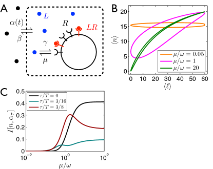
Figure S5: Predictive information in the module Eq. S25. (A) Schematic of the module. The response network consists of the equilibrium binding reaction only, cf. 1A. (B) Hysteresis in the response of the module to sinusoidal input $\alpha(t)=s(t)$. Note that in the saturating regime, the response is nonlinear. (C) Predictive information $\rho=0.5,\nu_{0}=10$ in the high-copy number limit, Eq. S27

Eq. S26 yields the predictive information $I(\tau)=I[n(t),\alpha(t+\tau)]$ without resorting to a Gaussian approximation. In a linear regime and for high ligand numbers, as detailed in the subsection Analytic results for predictive information below, we obtain

$$I(\tau)=\tfrac{1}{4}\rho^{2}\nu_{0}\delta^{2}\cos^{2}[(\tau+\Lambda)\omega]+O(\rho^{4}),$$ (S27)

where $\Lambda=\omega^{-1}\tan^{-1}(\omega/\mu)$ is the response lag time. As shown in Fig. S5C the module exhibits lagging optimal prediction above a critical $\tau_{c}=\cos^{-1}1/3\simeq 0.2T$, exploiting anticorrelated past signals $\tau+\Lambda\simeq T/2$ before the prediction target; this is the phase-matching strategy found already for exponential responders, Fig. 2A, as explained next.

A.8.1 Exploiting signal correlations through memory

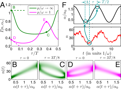
Figure S6: Prediction through memory. (A) For a range of prediction intervals $\tau$, frequency matching $\mu=\omega$ is more predictive than perfect tracking $\mu\to\infty$. The reason, as demonstrated by $p(n,\alpha_{\tau})$ at key points (B-E as indicated in A) and illustrated in F, is memory: receptors with $\mu=\omega$ time-convolve the signal, so that $n(t)$ lags by $\Lambda$; it is maximally correlated with $\alpha(t-\Lambda)$, which in turn mirrors $\alpha(t-\Lambda+T/2)$. Parameters are $\rho=0.75$ and $\nu_{0}=30$.

The reason why a lagging response helps long-term prediction is that it removes an ambiguity inherent the oscillatory signal, Fig. S6B-E. This mechanism is a realization of the general mechanism that an optimal response kernel emphasizes the most informative past signal values, in the particular case of a deterministic sinusoidal input signal and an exponential response, as in the minimal module Eq. S25.

While the fast response tracks the present input (B), its predictions suffer from a two-fold ambiguity about $\alpha(t+\tau)$, since a given value of $n(t)$ maps with high probability to two distinct values of $\alpha(t+\tau)$ whenever $\tau$ is not a multiple of $T/2$ (C). Indeed, the autocorrelation of a perfect sinusoidal input is $r_{\alpha}(t)=\cos(t/T)$, showing extrema at multiples of $T/2$. The frequency-matched response tracks the delayed signal $\alpha(t-\Lambda)$, since an exponential responder effectively delays a sinusoidal input signal by a constant shift $\Lambda$; this is a peculiarity of this signal/responder combination. This delayed tracking introduces ambiguity about the present signal for the same reason (D) but strikingly, helps prediction: The future signal $\alpha(t-\Lambda+T/2)$ is tracked without two-fold ambiguity (E), which maximizes predictive information. Indeed Eq. S27 shows that $I$ is maximal when the lag, advanced by half a period, equals the prediction interval, $-\Lambda+T/2=\tau$. For $\mu=\omega$, the lag is $\Lambda=T/8$ and the maximum is at $\tau=3T/8$. Counter-intuitively, then a frequency-matched responder contains even more information about the future ($\tau=3T/8$) than about the present, Fig. S6A. The effect of disambiguation is strong enough to outweigh the disadvantage of response damping ($I\propto\delta^{2}$, compare the ranges in C and E).

A.8.2 Details on fast ligand exchange

To identify the conditions for which ligand fluxes dominate over binding fluxes, we sum Eq. S26 over $n$, obtaining (here suppressing $t$ arguments)

$$\dot{p}(\ell)={\cal B}_{\ell}^{\alpha,\beta}p(\ell)+\gamma[\langle{}r|\ell_{+}\rangle\ell_{+}p(\ell_{+})-\langle{}r|\ell\rangle\ell p(\ell)]\\ +\mu[\langle{}n|\ell_{-}\rangle p(\ell_{-})-\langle{}n|\ell\rangle p(\ell)].$$ (S28)

For moderate driving amplitude around half-filling of the receptors, the conditional averages $\langle{}n|\ell\rangle,\langle{}r|\ell\rangle$ remain close to their mean $\nu_{0}$. Therefore, taking $\beta\gg\gamma\nu_{0}$ and $\alpha_{0}\gg\mu\nu_{0}$ ensures that $\dot{p}(\ell)\simeq{\cal B}_{\ell}p(\ell)$, i.e. the ligand in- and outflux terms dominate.

A.8.3 High copy-number limit

To gain intuition about the predictive performance of the module Eq. S25, we consider a high copy-number limit. We let $\{\lambda_{0},N\}\to\infty$ and $\gamma\to 0$ such that the mean number of bound receptors $\nu_{0}=\gamma\lambda_{0}N/\mu$ remains constant. This ensures that $n(t)$ remains in the linear, non-saturated range of the response curve: $N\gg\nu_{0}$ implies that $r(t)=O(N-\nu_{0})=O(N)$. It also ensures that the receptors are effectively driven by a deterministic signal: The relative width of the ligand distribution decreases as $\sigma_{\ell}/\lambda_{0}=O(\lambda_{0})^{-1/2}$. The receptor dynamics thus reduce to a birth-death process, $\partial_{t}p(n|t)={\cal B}_{n}^{\tilde{\gamma}(t),\mu}p(n|t)$, with effective birth rate $\gamma\ell(t)r(t)=\gamma[s(t)/\beta]N+O(\nu_{0}/N)+O(\lambda_{0}^{-1/2})$, which we denote as $\tilde{\gamma}(t)\equiv\gamma[s(t)/\beta]N=\nu_{0}\mu[1+\rho\cos(\omega t)]$. The solution to a birth-death process with time-dependent birth rate $\tilde{\gamma}(t)$ is a Poisson distribution Mugler et al. (2010) with mean

$$\langle{}n(t)\rangle=\int_{-\infty}^{0}\,dt^{\prime}e^{-\mu(t-t^{\prime})}\tilde{\gamma}(t^{\prime})=\nu_{0}\{1+\rho\delta\cos[\omega(t-\Lambda)]\},$$ (S29)

where the lag $\Lambda\equiv\tan^{-1}(\omega/\mu)/\omega$ and the damping $\delta\equiv[1+(\omega/\mu)^{2}]^{-1/2}$, as in the main text.

A.8.4 Analytic results for predictive information

For a deterministic signal $\alpha(t)$, we have $p(\alpha_{\tau}|n,t)=p(\alpha_{\tau}|t)=\delta[\alpha_{\tau}-\alpha(t+\tau)]$, and the predictive information becomes

$$I[n,\alpha_{\tau}]=$$

$$=\sum_{n}\int d\alpha_{\tau}\ p(n,\alpha_{\tau})\log\Bigl{[}\frac{p(n|\alpha_{\tau})}{p(n)}\Bigr{]}$$

$$=\sum_{n}\int d\alpha_{\tau}\oint dt\ p(\alpha_{\tau}|n,t)p(n|t)p(t)\log\Bigl{[}\frac{p(n|\alpha_{\tau})}{p(n)}\Bigr{]}$$

$$=\sum_{n}\frac{1}{T}\oint dt\ p(n|t)\log\Bigl{[}\frac{p(n|\alpha(t+\tau))}{p(n)}\Bigr{]}.$$ (S30)

For cosine driving $\alpha(t)=\alpha(T-t)$, there is a two-to-one relationship between $t$ and $\alpha$. This yields $p(n|\alpha(t+\tau))=[p(n|t_{1})+p(n|t_{2})]/2$, where $t_{1}=t$ and $t_{2}=T-t-2\tau$ are the two time points for which $\alpha_{\tau}$ takes on the value $\alpha(t+\tau)$. The predictive information becomes

$$I[n,\alpha_{\tau}]=\sum_{n}\frac{1}{T}\oint dt\ p(n|t)\log\Bigl{[}\frac{p(n|t_{1})+p(n|t_{2})}{2p(n)}\Bigr{]}.$$ (S31)

In the high copy-number limit (Figs. S5 and S6), Eq. S31 is evaluated numerically using the Poissonian $p(n|t)$ with mean $\langle{}n(t)\rangle=\nu_{0}\{1+\rho\delta\cos[\omega(t-\Lambda)]\}$, time lag $\Lambda\equiv\tan^{-1}(\omega/\mu)/\omega$, and damping factor $\delta\equiv[1+(\omega/\mu)^{2}]^{-1/2}$.

To get analytical insight, we can expand Eq. S31 in the limit of small driving amplitude $\rho$. To facilitate the expansion, we exploit the fact that $p(n|t)$ can be expressed Mugler et al. (2010) in terms of its Fourier modes in $t$,

$$p(n|t)=\sum_{z=-\infty}^{\infty}p_{n}^{z}e^{-iz\omega t},$$ (S32)

and its natural eigenmodes in $n$,

$$p_{n}^{z}=e^{iz\omega\Lambda}\sum_{j=0}^{\infty}\frac{(\nu_{0}\rho\delta/2)^{2j+|z|}}{j!(j+|z|)!}\phi_{n}^{2j+|z|}.$$ (S33)

Here $p_{n}^{z}=(1/T)\int_{0}^{T}dt\,e^{iz\omega t}p(n|t)$ are the components of the Fourier transform, which have support only at integer multiples $z$ of the driving frequency, and $\phi_{n}^{j}$ are the eigenmodes of the static birth-death process with mean bound receptor number $\nu_{0}$, i.e. $-{\cal B}_{n}^{\nu_{0},1}\phi_{n}^{j}=j\phi_{n}^{j}$ for eigenvalues $j\in\{0,1,\dots,\infty\}$ Walczak et al. (2009). Eq. S33 shows directly that the distribution is expressible as an expansion in the small parameter $\rho$. The remaining task is then to identify the leading term in $\rho$.

To identify the leading term in $\rho$, we insert Eq. S32 into Eq. S31, which yields

$$I = \frac{1}{T}\sum_{n}\int_{0}^{T}dt\ \sum_{z}p_{n}^{z}e^{-iz\omega t}$$ (S34)

$$\times\log\left\{\frac{1}{2p_{n}^{0}}\sum_{z^{\prime}}p_{n}^{z^{\prime}}\left[e^{-iz^{\prime}\omega t}+e^{-iz^{\prime}\omega(T-2\tau-t)}\right]\right\}.\qquad$$

Here we have recognized that $p(n)$, which is the time average of $p(n|t)$, is also the zeroth Fourier mode: $p(n)=\int_{0}^{T}dt\ p(n|t)p(t)=(1/T)\int_{0}^{T}dt\ p(n|t)=p_{n}^{0}$. Isolating the $z^{\prime}=0$ term and defining $q_{n}^{z}\equiv p_{n}^{z}e^{iz\omega\tau}$ to make the expression more symmetric yields

$$I = \frac{1}{T}\sum_{n}\int_{0}^{T}dt\ \sum_{z}p_{n}^{z}e^{-iz\omega t}$$ (S35)

$$\times\log\left\{1+\frac{1}{2p_{n}^{0}}\sum_{z^{\prime}\neq 0}q_{n}^{z^{\prime}}\left[e^{-iz^{\prime}\omega(t+\tau)}+e^{iz^{\prime}\omega(t+\tau)}\right]\right\},\qquad$$

where we have recognized that $e^{-iz^{\prime}\omega T}=1$. Then, recognizing that the term in brackets is symmetric upon $z^{\prime}\to-z^{\prime}$, we write the $z^{\prime}$ sum in terms of only positive integers,

$$I = \frac{1}{T}\sum_{n}\int_{0}^{T}dt\ \sum_{z}p_{n}^{z}e^{-iz\omega t}$$ (S36)

$$\times\log\left\{1+\frac{1}{2p_{n}^{0}}\sum_{z^{\prime}>0}r_{n}^{z^{\prime}}\left[e^{-iz^{\prime}\omega(t+\tau)}+e^{iz^{\prime}\omega(t+\tau)}\right]\right\},\qquad$$

where

$$r_{n}^{z} \equiv q_{n}^{z}+q_{n}^{-z}$$ (S37)

$$= e^{iz\omega\tau}p_{n}^{z}+e^{-iz\omega\tau}p_{n}^{-z}$$

$$= \left[e^{iz\omega(\Lambda+\tau)}+e^{-iz\omega(\Lambda+\tau)}\right]\sum_{j}\frac{(\nu_{0}\rho\delta/2)^{2j+|z|}}{j!(j+|z|)!}\phi_{n}^{2j+|z|}$$

$$= 2\cos[z\omega(\Lambda+\tau)]\sum_{j}\frac{(\nu_{0}\rho\delta/2)^{2j+|z|}}{j!(j+|z|)!}\phi_{n}^{2j+|z|}$$

is a real quantity.

Now, since $r_{n}^{z}$ is expressed in terms of our small parameter $\rho$, we Taylor expand the log in Eq. S36:

$$I = \frac{1}{T}\sum_{n}\int_{0}^{T}dt\ \sum_{z}p_{n}^{z}e^{-iz\omega t}\sum_{k=1}^{\infty}\frac{(-1)^{k+1}}{k}$$ (S38)

$$\times\left\{\frac{1}{2p_{n}^{0}}\sum_{z^{\prime}>0}r_{n}^{z^{\prime}}\left[e^{-iz^{\prime}\omega(t+\tau)}+e^{iz^{\prime}\omega(t+\tau)}\right]\right\}^{k}.\quad$$

It will turn out that the first two terms in the Taylor expansion will contribute to the leading order in $\rho$. The first term ($k=1$) is

$$I^{(1)} = \sum_{n}\frac{1}{2p_{n}^{0}}\sum_{z^{\prime}>0}r_{n}^{z^{\prime}}\sum_{z}p_{n}^{z}$$ (S39)

$$\times\frac{1}{T}\int_{0}^{T}dt\ e^{-iz\omega t}\left[e^{-iz^{\prime}\omega(t+\tau)}+e^{iz^{\prime}\omega(t+\tau)}\right],\qquad$$

where we have reordered terms in preparation for exploiting the relation $(1/T)\int_{0}^{T}dt\ e^{-i(z-z^{\prime})\omega t}=\delta_{zz^{\prime}}$. This relation turns the two terms in brackets into Kronecker deltas, which each collapse the sum over $z$, leaving

$$I^{(1)} = \sum_{n}\frac{1}{2p_{n}^{0}}\sum_{z^{\prime}>0}r_{n}^{z^{\prime}}\left(e^{-iz^{\prime}\omega\tau}p_{n}^{-z^{\prime}}+e^{iz^{\prime}\omega\tau}p_{n}^{z^{\prime}}\right)$$ (S40)

$$= \frac{1}{2}\sum_{n}\frac{1}{p_{n}^{0}}\sum_{z^{\prime}>0}(r_{n}^{z^{\prime}})^{2}.$$

In a completely analogous way, the second term in the Taylor expansion ($k=2$) reduces to

$$I^{(2)}=-\frac{1}{8}\sum_{n}\frac{1}{\left(p_{n}^{0}\right)^{2}}\sum_{x>0}\sum_{y>0}r_{n}^{x}r_{n}^{y}\left(r_{n}^{x+y}+r_{n}^{x-y}\right).$$ (S41)

Considering the $j=0$ term in $r_{n}^{z}$ (Eq. S37), it is clear that the leading order behavior in $\rho$, proportional to $\rho^{2}$, comes from the $z^{\prime}=1$ term in Eq. S40 and the $x=y=1$ term in Eq. S41:

$$I \approx \frac{1}{2}\sum_{n}\frac{1}{p_{n}^{0}}(r_{n}^{1})^{2}-\frac{1}{8}\sum_{n}\frac{1}{\left(p_{n}^{0}\right)^{2}}r_{n}^{1}r_{n}^{1}\left(r_{n}^{0}\right)$$ (S42)

$$= \frac{1}{2}\sum_{n}\frac{(r_{n}^{1})^{2}}{r_{n}^{0}}$$ (S43)

$$\approx \cos^{2}[\omega(\Lambda+\tau)]\left(\frac{\nu_{0}\rho\delta}{2}\right)^{2}\sum_{n}\frac{(\phi_{n}^{1})^{2}}{\phi_{n}^{0}}$$ (S44)

$$= \frac{\nu_{0}^{2}\rho^{2}}{4}\left[\frac{\cos(\omega\tau)-(\omega/\mu)\sin(\omega\tau)}{1+(\omega/\mu)^{2}}\right]^{2}\sum_{n}\frac{(\phi_{n}^{1})^{2}}{\phi_{n}^{0}}.\qquad$$ (S45)

Here, Eq. S43 uses the fact that $r_{n}^{0}=2p_{n}^{0}$ (Eq. S37), Eq. S44 takes only the $j=0$ term in Eq. S37, and Eq. S45 recalls that $\delta=[1+(\omega/\mu)^{2}]^{-1/2}$ and uses

$$\cos[\omega(\Lambda+\tau)] = \cos(\omega\Lambda)\cos(\omega\tau)-\sin(\omega\Lambda)\sin(\omega\tau)$$ (S46)

$$= \cos\left[\tan^{-1}(\omega/\mu)\right]\cos(\omega\tau)$$

$$-\sin\left[\tan^{-1}(\omega/\mu)\right]\sin(\omega\tau)$$

$$= \frac{1}{\sqrt{1+(\omega/\mu)^{2}}}\cos(\omega\tau)$$

$$-\frac{\omega/\mu}{\sqrt{1+(\omega/\mu)^{2}}}\sin(\omega\tau).$$

The sum in Eq. S45 is evaluated by noting that the zeroth eigenmode is a Poisson distribution with mean $\nu_{0}$ and that the first eigenmode is related to the zeroth eigenmode via $\phi_{n}^{1}=\phi_{n-1}^{0}-\phi_{n}^{0}=\phi_{n}^{0}(n-\nu_{0})/\nu_{0}$ Mugler et al. (2009). The sum therefore becomes $(1/\nu_{0}^{2})\sum_{n}\phi_{n}^{0}(n-\nu_{0})^{2}$, which is the variance of the Poisson distribution (equal to $\nu_{0}$) divided by $\nu_{0}^{2}$, or $1/\nu_{0}$. Altogether, then, Eq. S45 becomes

$$I=\frac{\nu_{0}\rho^{2}}{4}{\left[\frac{\cos(\omega\tau)-(\omega/\mu)\sin(\omega\tau)}{1+{(\omega/\mu)}^{2}}\right]}^{2},$$ (S47)

as in Eq. S27.

A.8.5 Robustness to low copy-number effects

We here relax the assumption of high copy number and solve numerically the full description of the system given by Eq. S26. We find that lagging prediction remains optimal as the mean ligand number $\lambda_{0}$ and the total receptor number $N$ are reduced, even down to $\lambda_{0}=1$ (Fig. S7A) and $N=1$ (Fig. S7B). As $N$ is reduced, the information is reduced for all values of the response rate $\mu$ (B), since reducing $N$ compresses the response range. As $\lambda_{0}$ is reduced, the information is largely unchanged (A); this is because ligand exchange remains faster than the driving dynamics ($\beta/\omega\gg 1$), meaning that even a small number of ligand molecules can cycle in and out of the system many times over a period. In both cases, there remains an optimum in the predictive information as a function of $\mu$ located in the regime $\mu\simeq\omega$, illustrating that lagging optimal prediction persists even at low copy numbers.

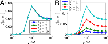
Figure S7: Lagging optimal prediction persists (A) for low mean ligand number $\lambda_{0}$ and (B) for low total receptor number $N$. The minimal module Eq. S25 is driven by sinusoidal input $\alpha(t)$. Parameters are $\tau=3T/8$, $\rho=0.5$, $\beta/\omega=100$, $\gamma=\mu/\lambda_{0}$, and, in A, $N=5$ and, in B, $\lambda_{0}=5$. In A, all curves closely overlap.

A.8.6 Lagging optimal prediction of diverse input signals

Lagging prediction is a robust strategy for non-Markovian signals, beyond Gaussian signals and linear response. Fig. S8A shows the benefit of a slow response for prediction for two-state switching signals $\alpha(t)=\alpha_{0}(1\pm\rho)$ with random switching times that are Gamma-distributed with shape parameter $k$ and mean $T/2$. The minimal module’s response strongly distorts the rectangular signal shape, but lagging prediction remains optimal for all $k\geq 3$, Fig. S8A.

Eq. S27 demonstrates optimal lagging prediction for non-Gaussian (deterministic) input at constant amplitude. The effect persists also at low copy numbers. Fig. S8B shows lagging optimal prediction for $I[n(t),\alpha(t+\tau)]$ in the minimal module Eq. S25, driven by NM signals as defined above, at $N=25$, but the effect persists even for ligand or receptor numbers down to 5 (not shown).

Figure S8: Lagging optimal prediction is generic. (A) For stochastic two-state driving with Gamma-distributed waiting times, lagging prediction is optimal for shape parameters $k\geq 3$. The mean waiting time is held constant at $T/2$. (B) For a noisy harmonic oscillator signal, fast prediction is optimal in the overdamped regime $\eta\geq 2$. In the underdamped regime, lagging, frequency-matched prediction again becomes optimal. Parameters are $\tau=3T/8$, $\rho=0.5$, $\lambda_{0}=25$, $N=25$, $\beta/\omega=100$, and $\gamma=\mu/\lambda_{0}$. Simulation details are given in the last section of this supplement.

A.8.7 Ligand binding simulation parameters and details

The data for Figs. S8A and B were generated by a Gillespie-type kinetic Monte Carlo simulation. Dynamic ligand birth rates $\alpha(t)$ were approximated as constant during short discretization intervals of length $\tau_{\alpha}=T/50$; after each such interval, queued next reaction times were erased and re-generated according to the new value of the rate. This is an exact simulation procedure for the approximated system with stepwise-constant rate.

For the two-state driving protocol (Fig. S8A), the mean ligand number and total receptor number were set to $\lambda_{0}=N=25$. The ligand death rate was set to $\beta=100$, and the mean driving period was set to $T=2\pi$ in simulation time units. Switching times were generated independently, following a Gamma- (or Erlang-) distribution with shape parameter $k\in\{1,2,3,5,10,20,50\}$ and mean $T/2$. The input rate was set to a random initial value $\alpha_{0}[1\pm\rho]$ and then toggled after each random switching time between $\alpha_{0}[1\pm\rho]$, where $\alpha_{0}=\lambda_{0}\beta$ and $\rho=0.5$. For a given ligand dissociation rate constant $\mu$, the association constant was set to $\gamma=\mu/\lambda_{0}$ to ensure half-filling at the average driving rate.

For the harmonic-oscillator protocol (Fig. S8B) the same parameters were used, except that the driving signal was now generated by a forward-Euler integration of the Langevin equation given in the main text. The damping parameter $\eta$ was varied in $\{1/2,1,2,4\}$.

For each value of $\mu$, the system state was initialized to the equilibrium molecule numbers at $\alpha=\alpha_{0}$, and $N_{\mathrm{tr}}=2000$ trajectories of length $10T$ were generated.

Trajectories were sampled at discrete time intervals $T/100$, and the corresponding samples of the input rate were binned. The input-output mutual information was estimated by applying the definition $I[x,y]=\langle{}\log\frac{p(x,y)}{p(x)p(y)}\rangle$ to the binned simulation data. In doing so, the choice of bin size for the continuous variable $\alpha$ (in the harmonic-oscillator case) can lead to systematic errors; we found the results for $I$ to be independent of the bin size in a plateau region around $N_{\mathrm{bin}}=100$ equally filled bins, and therefore used this binning for Fig. S8B.

The data were split into 10 blocks of 200 trajectories each and the mutual information $I[n,\alpha_{\tau}]$ for various prediction intervals $\tau\in[0,T/2]$ were calculated based on histograms of the discrete-valued samples, for each block. Plots show the averages over blocks together with standard errors of the mean estimated from block-wise variation.

A.9 E. coli chemotaxis simulations

To explore the role of prediction in chemotaxis, we set up a stochastic simulation of E. coli swimming in a concentration field in two dimensions. E. coli performs the well-known chemotaxis behavior Berg (2004) of alternating runs and tumbles. During a tumble phase, the bacterium remains stationary, reorients in a random direction and initiates a new run with constant propensity $\beta=10/{\rm s}$. Runs then proceed with constant velocity $v_{0}=20\mu{\rm m/s}$. They are governed by the Langevin equation

$$d\vec{r}(t) =v_{0}\,(\cos\phi,\sin\phi)\,dt,$$

$$d\phi(t) =\sqrt{2D_{\text{rot}}}\,dw(t),$$ (S48)

where $dw(t)$ is standard Gaussian white noise and affects the orientation $\phi$ with a rotational diffusion constant $D_{\text{rot}}=0.15\,\mathrm{rad^{2}/s}$.

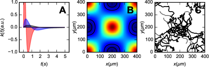
Figure S9: Chemotaxis in E. coli. (A) Linear chemotactic response kernel $k$ as measured in Segall et al. (1986) (blue), and rescaled $k_{5}$ (red) and $k_{1/2}$ (black) versions. (B) Egg-crate potential, varying from 0 (blue) to 2 (red) in arbitrary units. (C) Example trajectory of a chemotaxing bacterium (solid line) with some virtual continued runs (dashed, see text).

Runs end with tumbling events, which have a propensity (tumbling rate)

$$\alpha(t)=\alpha_{0}\max[0,1-x(t)];\;x(t)=\int_{-\infty}^{t}k(t-t^{\prime})\ell(t^{\prime})dt^{\prime}.$$ (S49)

The base tumbling rate $\alpha_{0}=1/{\rm s}$. The tumbling rate is modulated as a function of the signal history via the linear-response kernel $k(t)$, which generates the chemotaxis pathway output $x(t)$. That is, the kernel $k$ summarizes the dynamics of the chemotaxis network including phosphorylation of CheYp by CheA, modulation of CheA activity by the receptor, and receptor-activity modulation via receptor-ligand binding and receptor methylation and demethylation Shimizu et al. (2010), in a linear regime.

Following Celani and Vergassola (2010), we use for $k(t)$ the clockwise-bias kernel as measured on tethered bacteria Block et al. (1982); Segall et al. (1986). (Although this is not fully rigorous, determining the actual rate kernel Block et al. (1982) would require additional assumptions, and tends to result in similar kernel shapes [not shown]). For ease of use in the simulations, we fit the kernel to $k(t)=be^{-at}(t-(a/2)t^{2})$ where the data in Segall et al. (1986) yield $b=A\times 2.91$ and $a=2.05/s$. The sensitivity $A=200/{\rm s}$ controls the degree of tumbling rate modulation; we obtain a range of roughly $0<\alpha(t)\lesssim 3\alpha_{0}$ similar to what is reported in Segall et al. (1986).

Importantly, the kernel $k$ has the property of perfect adaptation $\int_{0}^{\infty}k(t)dt=0$, which implies, among other advantages, that it is insensitive to the constant background concentration level. As the kernel shape suggests (Fig. S9A), the output is a smoothed finite-time derivative of the input. Here, we do not attempt to derive a globally optimal shape, but start with the observation that the kernel is adaptive, and ask how the optimal speed of the kernel depends on the noise. We do this by comparing rescaled kernels $k_{\nu}(t)=\nu^{2}k(\nu t)$ of varying response speed $\nu$. With the chosen amplitude scaling, $\int k_{\nu}(t-t^{\prime})\ell(t^{\prime})dt^{\prime}\to\int|k(t)|dt\times\dot{\ell}(t)$ as $\nu\to\infty$, i.e. in this limit the kernel acts as the instantaneous input derivative.

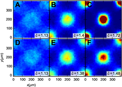
Figure S10: Chemotaxis in an egg-crate potential. Average concentration $\bar{c}$ at noise $\theta=0$ (A-C) and at noise $\theta=2$ (D-F). The slow kernel $k_{1/2}$ (A,D) has a low performance due to a lack of response speed, but is robust to noise. The fast kernel $k_{3}$ (C,F) shows the highest localization, even though it is strongly affected by noise. The wild-type kernel $k_{1}$ (B,E) shows intermediate behavior.

Simulated E. coli bacteria chemotax in a $L\times L$ concentration field with periodic boundary conditions of size $L=400\mu\mathrm{m}$, with concentrations given by a sinusoidal egg-crate function $c(x,y)=1+\cos(2\pi x/L)\cos(2\pi y/L)$ ($c$ is unit-less; see Fig. S9B). The signal $s(t)$ is the ligand concentration: $s(t)=c[\vec{r}(t)]$. In this parameter regime, the resulting input signal is not oscillatory: the correlation function decays monotonically (but not exponentially, not shown).

To appreciate the role of input noise, we compare the case without noise in the input signal, with the scenario where due to a low concentration of ligand, the noise is dominated by the input noise, and the intrinsic noise can be neglected, as in our theory. For the latter case, we now determine a reasonable noise strength. The input signal of the chemotaxis system is the activity $A\propto\ell$ of the receptor molecules that bind the ligand. Input noise arises from receptor-ligand binding and/or the conformational dynamics of the receptor molecules. Since we disregard intrinsic noise, only the relative noise strength matters, as well as its correlation time, as discussed previously. If there are a total of $R_{T}$ independent receptor units that switch between an active and an inactive state, then the relative variance $\sigma^{2}_{A}/\langle{}A\rangle^{2}=R_{T}p(1-p)/(R_{T}p)^{2}\simeq(R_{T}p)^{-1}$, where $p$ is the (small) average activity of a receptor unit. With a dissociation constant of $K_{D}\simeq 0.1-1\mu{\rm M}$ Vaknin and Berg (2007), a concentration $c\simeq 1{\rm nM}$ yields a receptor occupancy (and we assume, activity) of $p\approx 0.001-0.01$. We assume that $R_{T}$ is given by the number of receptor-CheA complexes, yielding $R_{T}\approx 1000$ Li and Hazelbauer (2004). Moreover, we assume that the correlation time is given by that of receptor-ligand binding, $\tau_{A}=1/(k_{\rm on}c+k_{\rm off})$, where $k_{\rm on}$ and $k_{\rm off}$ are the receptor-ligand association and dissociation rates, respectively. These assumptions most likely give a lower bound on the noise, because cooperative interactions between receptors Skoge et al. (2013) and diffusion of ligand Wang et al. (2007) introduce spatio-temporal correlations between the receptors. With a dissociation constant $K_{D}=0.1\mu{\rm M}$ and an association rate of $k_{\rm on}=10^{9}{\rm M}^{-1}{\rm s}^{-1}$ Danielson et al. (1994), the dissociation rate is $k_{\rm off}\approx 100{\rm s}^{-1}$, which yields a correlation time $\tau_{A}\approx 10{\rm ms}$. We then arrive at an integrated noise strength relative to the signal of $\sigma^{2}_{A}\tau_{A}/\langle{}A\rangle^{2}\approx 1-10{\rm ms}$. The effect of noise on the network output is determined by the relative integrated noise strength $\tau_{A}\sigma_{A}^{2}/\langle{}A\rangle^{2}$. In our simulations, we use a time step of $dt=2{\rm ms}$; to replicate the noise strength we thus generate the network input $\ell=s+\xi$ by adding to the signal at each time step an independent Gaussian random number $\xi$ of relative variance $\theta^{2}\equiv\sigma_{\xi}^{2}/\langle{}s\rangle^{2}=(\tau_{A}/dt)/(pR_{T})\approx 0.5-5$. As a representative relative noise we have finally chosen $\theta=2$.

The simulation proceeds by random reorientation followed by Euler forward integration of Eq. A.9 during run phases, and simultaneously, updates of the pathway output $x(t)$ during run and tumble phases. Tumble/restart events are generated via the procedure described in Ref. van Albada and ten Wolde (2009). Fig.S9C shows an example trajectory segment.

As a result of the chemotactic mechanism, the simulated bacteria move on average towards regions of higher input concentration, as indicated by the long-term average concentration $\bar{c}=\langle{}s\rangle$, which exceeds the random value, $\bar{c}=1$, see Fig. S10.

A.9.1 Coarse-grained description as biased diffusion

The stationary distribution does not show the speed at which the concentration maxima are approached by the bacteria. To measure the speed, we calculated the average, coarse-grained chemotactic speed on the time scale $\delta t$ as

$$\vec{v}_{\delta t}(\vec{r})=\langle{}\vec{r}(t+\delta t)-\vec{r}(t)\rangle_{\vec{r}}/\delta t,$$ (S50)

where the subscript indicates that the average is taken over trajectories that pass through $\vec{r}$ at $t$. Generally speaking, the choice of mesoscopic time scale $\delta t$ affects the measured chemotactic speeds when $\delta t$ is smaller than than a typical run length; however too large $\delta t$ will include effects from the curvature of the underlying concentration field. We chose $\delta t=4\mathrm{s}$ as a reasonable compromise; results from 2s to 8s are similar.

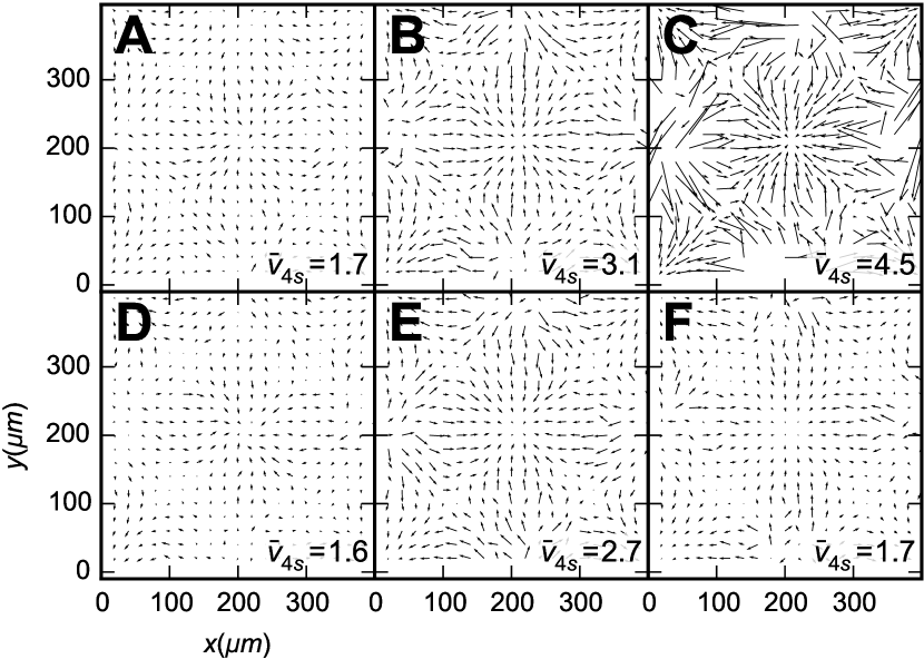
Figure S11: Coarse-grained local velocity $v_{\delta t}$ in $\mu\mathrm{m}/\mathrm{s}$ with time-step $\delta t=4\mathrm{s}$. As in Fig. S10, noise levels are $\theta=0$ (A-C), $\theta=2$ (D-F), and kernel speeds are $\nu=1/2$ (A,D), $\nu=1$ (B,E) and $\nu=3$ (C,F), respectively.

This vector field is shown in Fig. S11. Clearly, at $\theta=0$, the mean speed increases as the kernel integration time decreases; however at finite noise $\theta=2$, there is a speed optimum for the wildtype-speed kernel in panel (E). The average uphill speed, defined as the average projection of $v_{\delta t}$ in the direction of the positive concentration gradient,

$$\bar{v}_{\delta t}=\Bigl{\langle}\frac{\vec{v}_{\delta t}(\vec{r})\cdot\nabla c(\vec{r})}{\|\nabla c(\vec{r})\|}\Bigr{\rangle},$$ (S51)

shown in the insets, confirms this observation.

The question arises why localization efficiency at high noise stays high for the fast kernel $k_{3}$ (Fig. S10), while the drift speed towards the maxima actually decreases. This can be understood by considering that both the chemotactic speed and the localization are affected by the typical run length. Namely, if runs become shorter, the chemotactic speed decreases because random reorientations occur more often. At the same time, with shorter runs, smaller features of the concentration field can be resolved, increasing the potential for good localization. Indeed we find that unfiltered noise $\theta=2$ induces many tumbles for the fast kernel $k_{3}$, decreasing the mean run length to 0.55s, whereas in all other conditions, the mean run length remains close to the unperturbed value 1s. Thus, short runs allow slow but in a static concentration field eventually successful, chemotaxis.

A.9.2 Predictive information in chemotaxis

To chemotax, bacteria modulate the run lengths. Since a tumbling rate bias at the current time comes into effect only at the next tumbling event, this means that the current modulation of the tumbling rate should take into account the future ligand concentration until the end of the run, around $\alpha_{0}^{-1}=1{\rm s}$ in the future. In other words, E. coli needs to predict future ligand concentration. To elucidate what precise kind of predictive information is most relevant for chemotaxis, and to relate it to chemotactic performance, we measured predictive information in our simulations.

Since E. coli reacts to its own predictions by tumbling, correlating the current signaling output with the future concentrations along its trajectory would include the feedback loop between prediction and motile response. To assess how reliably E. coli can predict the future concentration, we thus need to decouple the estimation of the future concentration from the response to the estimate, which is the tumble event. We do this by constructing virtual trajectories (shown as dotted lines in Fig. S9C), which are obtained by prolonging a run for a set amount of time after a tumble event. Along these virtual runs we then compute the predictive information between the output $x(t)$ at a given point in time $t$, and either the future signal $s(t+\tau)$ or the future change in signal $s(t+\tau)-s(t)$. It is this predictive information that allows E. coli to estimate the benefit of postponing or advancing the next tumble event.

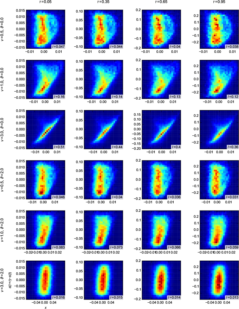
Figure S12: Histograms of the predictive joint distribution $p(x,s_{\tau}-s)$. Noise level $\theta=0,2$ and speeds $\nu=0.5,1,3$, from top to bottom; increasing prediction intervals $\tau$, left to right. Response amplitude $A=200$; predictive informations $I=I[s_{\tau}-s,x]$ as indicated.

Fig. S12 shows two-dimensional histograms of output $x(t)$ and future input change $s_{\tau}-s$ for various values of the prediction interval $\tau$. Without noise and for the fast kernel $k_{3}$, the diagonal shape at low $\tau$ indicates that the finite-time derivative taken by the kernel, predicts the future change with good accuracy; slower kernels show this feature to a weaker extent. As $\tau$ increases, two effects are visible: expansion along the vertical axis, due to the longer runs for larger $\tau$; and blurring of the diagonal, which results from the finite length scale of the potential. (Since we consider virtual runs, tumbling does not contribute to uncertainty about the future concentration.) At high noise, the diagonal is much weaker, and the horizontal axis scale is higher; both of these effects result from noise adding large random contributions to the output. The effect is particularly strong for the fast kernel.

From histograms as in Fig. S12 we estimated mutual information by taking the sum over bins at index $i,j$

$$I_{N}^{M}=\sum_{i,j=1}^{N,N}h(i,j)\log[h(i,j)/h(i)h(j)]$$ (S52)

where $h$ denotes bin counts normalized by the total sample number $M$, or row and columns counts, respectively. Since this estimator is prone to bias, we used a procedure Cheong et al. (2011) of subsampling the data to various $M$, and linearly extrapolating the data points $(1/M,I_{N}^{M})$ to $1/M\to 0$. Error bars were derived from this extrapolation. We verified that the resulting estimate was consistent for a range of bin numbers $N$.

The resulting predictive information values as a function of the prediction interval $\tau$ are shown in Fig. 4 in the main text, where the predicted variable is the future concentration change. In Fig. S13 we show the corresponding result for the predictive information $I[x,s_{\tau}]$ between the current output $x(t)$ and the future input signal itself, $s(t+\tau)$ (rather than the change $s(t+\tau)-s(t)$). Clearly the predictive information about the future signal value does not correlate with chemotactic efficiency. The results of Figs. 4 and S13 together show that the search strategy of E. coli is based on predicting the future change in the signal, rather than the signal itself.

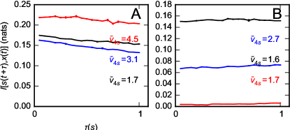
Figure S13: Predictive power $I[x,s_{\tau}]$ between $x(t)$ and $s(t+\tau)$ vs. forecast interval $\tau$ for the original E. coli kernel with $\nu=1$, for a faster kernel with $\nu=3$ and a slower kernel with $\nu=0.5$, for two different noise levels.

References

- Bergstrom and Lachmann (2005) C. T. Bergstrom and M. Lachmann, “The fitness value of information,” (2005), arXiv:0510007 [q-bio.PE] .
- Taylor et al. (2007) S. F. Taylor, N. Tishby, and W. Bialek, “Information and fitness,” (2007), arXiv:0712.4382 [q-bio.PE] .
- Bialek (2012) W. Bialek, Biophysics: Searching for Principles (Princeton Univ Pr, 2012).
- Balaban et al. (2004) N. Q. Balaban, J. Merrin, R. Chait, L. Kowalik, and S. Leibler, Science 305, 1622 (2004).
- (5) See supplementary information.
- Mitchell et al. (2009) A. Mitchell, G. H. Romano, B. Groisman, A. Yona, E. Dekel, M. Kupiec, O. Dahan, and Y. Pilpel, Nature 460, 220 (2009).
- Tagkopoulos et al. (2008) I. Tagkopoulos, Y.-C. Liu, and S. Tavazoie, Science 320, 1313 (2008), PMID: 18467556.
- Kaupp et al. (2008) U. B. Kaupp, N. D. Kashikar, and I. Weyand, Annual Review of Physiology 70, 93 (2008).
- Valencia et al. (2012) J. Valencia, S., K. Bitou, K. Ishii, R. Murakami, M. Morishita, K. Onai, Y. Furukawa, K. Imada, K. Namba, and M. Ishiura, Genes to Cells 17, 398 (2012).
- Berg and Purcell (1977) H. C. Berg and E. M. Purcell, Biophysical Journal 20, 193 (1977).
- Bialek and Setayeshgar (2005) W. Bialek and S. Setayeshgar, Proceedings of the National Academy of Sciences of the United States of America 102, 10040 (2005), PMID: 16006514.
- Govern and ten Wolde (2012) C. C. Govern and P. R. ten Wolde, Physical Review Letters 109, 218103 (2012).
- Mehta and Schwab (2012) P. Mehta and D. J. Schwab, Proceedings of the National Academy of Sciences (2012), 10.1073/pnas.1207814109.
- Kaizu et al. (2014) K. Kaizu, W. de Ronde, J. Paijmans, K. Takahashi, F. Tostevin, and P. R. ten Wolde, Biophysical Journal 106, 976 (2014).
- Govern and ten Wolde (2014) C. C. Govern and P. R. ten Wolde, Proceedings of the National Academy of Sciences of the United States of America 111, 17486 (2014).
- Govern and ten Wolde (2014) C. C. Govern and P. R. ten Wolde, Phys Rev Lett 113, 258102 (2014).
- Aquino et al. (2014) G. Aquino, L. Tweedy, D. Heinrich, and R. G. Endres, Scientific Reports 4 (2014), 10.1038/srep05688.
- Heinrich et al. (2002) R. Heinrich, B. G. Neel, and T. A. Rapoport, Molecular Cell 9, 957 (2002).
- Tănase-Nicola et al. (2006) S. Tănase-Nicola, P. B. Warren, and P. R. ten Wolde, Physical Review Letters 97, 068102 (2006).
- Ziv et al. (2007) E. Ziv, I. Nemenman, and C. H. Wiggins, PLoS One 2, e1077 (2007).
- de Ronde et al. (2010) W. H. de Ronde, F. Tostevin, and P. R. ten Wolde, Physical Review E 82, 031914 (2010).
- Hinczewski and Thirumalai (2014) M. Hinczewski and D. Thirumalai, Physical Review X 4, 041017 (2014).
- Alon (2006) U. Alon, An Introduction to Systems Biology: Design Principles of Biological Circuits, 1st ed. (Crc Pr Inc, 2006).
- Wiener (1950) N. Wiener, Extrapolation, interpolation, and smoothing of stationary time series (Wiley, 1950).
- Kolmogorov (1992) A. N. Kolmogorov, Selected Works of A. N. Kolmogorov: Probability theory and mathematical statistics (Springer Science & Business Media, 1992).
- Kondo (1997) T. Kondo, Science 275, 224 (1997).
- Kholodenko (2000) B. N. Kholodenko, European journal of biochemistry / FEBS 267, 1583 (2000).
- Sasagawa et al. (2005) S. Sasagawa, Y.-i. Ozaki, K. Fujita, and S. Kuroda, Nat Cell Biol 7, 365 (2005).
- Segall et al. (1986) J. E. Segall, S. M. Block, and H. C. Berg, Proc Natl Acad Sci U S A 83, 8987 (1986).
- Block et al. (1982) S. M. Block, J. E. Segall, and H. C. Berg, Cell 31, 215 (1982).
- Celani and Vergassola (2010) A. Celani and M. Vergassola, Proc Natl Acad Sci U S A 107, 1391 (2010).
- Berg (2004) H. Berg, E. in motion, Biological and Medical Physics Biomedical Engineering (Springer, New York, 2004).
- Bialek et al. (2001) W. Bialek, I. Nemenman, and N. Tishby, Neural Comput 13, 2409 (2001).
- Tostevin and ten Wolde (2009) F. Tostevin and P. R. ten Wolde, Phys Rev Lett 102, 218101 (2009).
- Cover and Thomas (2012) T. M. Cover and J. A. Thomas, Elements of information theory (John Wiley & Sons, 2012).
- Tostevin and ten Wolde (2010) F. Tostevin and P. R. ten Wolde, Phys Rev E Stat Nonlin Soft Matter Phys 81, 061917 (2010).
- Mugler et al. (2010) A. Mugler, A. M. Walczak, and C. H. Wiggins, Phys. Rev. Lett. 105, 058101 (2010).
- Walczak et al. (2009) A. M. Walczak, A. Mugler, and C. H. Wiggins, Proceedings of the National Academy of Sciences 106, 6529 (2009).
- Mugler et al. (2009) A. Mugler, A. M. Walczak, and C. H. Wiggins, Phys. Rev. E 80, 41921 (2009).
- Shimizu et al. (2010) T. S. Shimizu, Y. Tu, and H. C. Berg, Mol Syst Biol 6, 382 (2010).
- Vaknin and Berg (2007) A. Vaknin and H. C. Berg, Journal of Molecular Biology 366, 1416 (2007).
- Li and Hazelbauer (2004) M. Li and G. L. Hazelbauer, Journal of Bacteriology 186, 3687 (2004).
- Skoge et al. (2013) M. Skoge, S. Naqvi, Y. Meir, and N. S. Wingreen, Physical Review Letters 110, 248102 (2013).
- Wang et al. (2007) K. Wang, W.-J. Rappel, R. Kerr, and H. Levine, Phys Rev E Stat Nonlin Soft Matter Phys 75, 061905 (2007).
- Danielson et al. (1994) M. A. Danielson, H.-P. Biemann, D. E. Koshland, and J. J. Falke, Biochemistry 33, 6100 (1994).
- van Albada and ten Wolde (2009) S. B. van Albada and P. R. ten Wolde, PLoS Comput Biol 5, e1000378 (2009).
- Cheong et al. (2011) R. Cheong, A. Rhee, C. J. Wang, I. Nemenman, and A. Levchenko, Science 334, 354 (2011).