Power spectrum of flow fluctuations in relativistic heavy-ion collisions

Abstract

We carry out hydrodynamical simulation of the evolution of fluid in relativistic heavy-ion collisions with random initial fluctuations. The time evolution of power spectrum of momentum anisotropies shows very strong correspondence with the physics of cosmic microwave anisotropies as was earlier predicted by us. In particular our results demonstrate suppression of superhorizon fluctuations and the correspondence between the location of the first peak in the power spectrum of momentum anisotropies and the length scale of fluctuations and expected freezeout time scale (more precisely, the sound horizon size at freezeout).

It has been recognized for some time now that there are deep interconnections between the evolution of flow anisotropies in relativistic heavy-ion collision experiments (RHICE) and the physics of inflationary density fluctuations observed as cosmic microwave background radiation (CMBR) anisotropies. Analogies between the last scattering surface for CMBR and the freezeout surface in RHICE were always mentioned, however these remained at a motivational level. A rigorous correspondence in the physics of the two systems was first made by us in ref.cmbhic where it was pointed out for the first time that instead of focusing on first few flow coefficients (which, until that time, were primarily only even flow coefficients $v_{2},v_{4},v_{6}$) one should plot the entire power spectrum of all flow coefficients including the odd coefficients. The reason for departure from conventional focus on only first few even flow coefficients was the recognition that initial state fluctuations contribute to development of all flow coefficients (including the odd ones) even for central collisions. Many subsequent investigations confirmed this expectation flowfluct ; srnsn and indeed now one routinely measures odd coefficients (e.g. the triangular flow coefficient $v_{3}$) and there have also been several investigations of power spectrum of flow coefficients upto a large value of $n$ of about 10-12.

In this work we present results of hydrodynamic simulations of the evolution of flow fluctuations and focus on the physics of various features of the power spectrum keeping in mind the very rich possibilities of correspondence with the power spectrum of CMBR anisotropies. Some of the most important features of CMBR power spectrum are the presence of acoustic peaks, the relation between the location of the first peak and the horizon size at last scattering surface, and the suppression of power in superhorizon modes. These are intimately connected to the fact the density fluctuations of the universe originate during an early phase of inflation where causally generated fluctuations are stretched to superhorizon scales. We study these aspects in RHICE using hydrodynamic simulations. We study the evolution of power spectrum of momentum anisotropies $v_{n}$ (root mean square values $v_{n}^{rms}$ of $v_{n}$s) and contrast it with the power spectrum of initial spatial anisotropies $F_{n}$ (root mean square values $F_{n}^{rms}$ of $F_{n}$s). We find that for large values of $n$, the two power spectrum correlate reasonably well. However for $n$ smaller than a specific value (about 3-4 for the cases studied by us) there are significant differences. While plot of $F_{n}^{rms}$ keeps monotonically rising with decreasing $n$, the plot of $v_{n}^{rms}$ starts dropping below $n\sim 3-4$. In cmbhic we had predicted this using the concept of superhorizon fluctuations, as spatial anisotropies larger than a specific wavelength are not fully transferred to the momentum anisotropies due to insufficient time for flow development from pressure gradients over the relevant length scales. The first peak therefore contains the information about the longest wavelength of fluctuations at the freezeout surface. We next consider initial fluctuations of specific wavelengths and study the shift of the first peak as the size of initial fluctuations is varied. We find that for larger (smaller) initial fluctuations the peak shifts to smaller (larger) $n$ roughly by the same scale factor. Further, for a fixed initial size of spatial fluctuations, we find that the first peak in the power spectrum of momentum anisotropies keeps shifting to lower values of $n$ as time increases. Nature of this shift is entirely consistent with the increasing size of the sound horizon with time. The nature and location of the first peak in the power spectrum of flow anisotropies thus contains rich information about the initial fluctuation spectrum, their evolution, and the freezeout time scale. We also study time evolution of $v_{n}$s at different $n$ and show that oscillations set in for larger values of $n$ early on just as happens for acoustic oscillations in CMBR power spectrum. For CMBR power spectrum even the ratios of different peaks contains important information, e.g. baryon to dark matter ratio. Here, for the single fluid dynamics we have studied, we find that the ratio of first peak to 2nd peak directly relates to the scale of initial fluctuations. For multifluid case, with particle species specific power spectra, different peak ratios may yield important information for different fluid components of the plasma. Our results confirm the expectation that there is a deep correspondence between the evolution of fluctuations in RHICE and that in the early universe. With phenomenal success of CMBR power spectrum analysis in providing detailed information about the very early history of the universe, this should provide ample motivation for detailed investigations of the power spectrum of flow fluctuations in RHICE for probing the very early stages of plasma evolution.

We have developed two independent codes for hydrodynamic simulations. One is a 2+1 dimensional code in the framework of Bjorken’s longitudinal scaling expansion model and uses leapfrog algorithm of 4th order accuracy with a trapezoidal correctionzalesak . The initial conditions for this simulation are generated using a Wood-Saxon background plus fluctuations obtained using Glauber Monte Carlo gbmc where a nucleus-nucleus collision is viewed as a sequence of independent binary nucleon-nucleon collisions. The total energy density calculated using Glauber optical initial condition for the same parameters is distributed equally among the binary collisions as Gaussian fluctuations (plus the Wood-Saxon part). A lattice equation of state is used for the evolution of the plasma.

The second code is a full 3+1 dimensional code. This uses leapfrog algorithm of 2nd order accuracy and uses QGP ideal gas equation of state for 2 massless flavors. The flow become unstable for large velocities. In regions of negligible energy density we artificially put an upper cutoff (of 0.95) on the fluid speed. When regions with significant energy density start developing instabilities, simulation is stopped. The initial conditions here are provided in terms of a Wood-Saxon background plus randomly placed Gaussian fluctuations of specific widths. In order to compare with the results with first code, only central rapidity region is used for calculation of flow fluctuations using transverse coordinates and momenta. We will present results from this second simulation as it provides a direct control of spectrum of initial fluctuations. This way specific patterns observed in the final power spectrum can be correlated with the properties of initial fluctuations. We have compared each of these results with the 2+1 dimensional code (by utilizing partial control over density fluctuations in the Glauber model in terms of energy density deposition in each binary collision) and results of both simulations show similar patterns.

We use same methods for calculating spatial and flow anisotropies as in our earlier work cmbhic . We will use $F_{n}$ to denote Fourier coefficients for the spatial anisotropies, and use the conventional notation $v_{n}$ to denote $n_{th}$ Fourier coefficient of the resulting momentum anisotropy in ${\delta p}/p$. We do not calculate the average values of the flow coefficients $v_{n}$, instead we calculate root-mean square values of the flow coefficients $v_{n}^{rms}$. Further, these calculations are performed in a lab fixed frame, without any reference to the event planes of different events. Average values of $v_{n}$ are zero due to random orientations of different events. As $v_{n}^{rms}$ will have necessarily non-zero values, physically useful information will be contained in the non-trivial shape of the power spectrum (i.e. the plot of $v_{n}^{rms}$ vs. $n$). More precisely, our focus will be on the structure of the peaks of the plot and evolution of oscillations in this plot as a function of time. Momentum anisotropies are calculated by calculating transverse momentum density at each point from the evolving fluid energy momentum tensor. Spatial anisotropies are estimated by calculating the anisotropies in the fluctuations in the spatial extent $R(\phi)$ at any given stage, where $R(\phi)$ represents the energy density weighted average of the transverse radial coordinate in the angular bin at azimuthal coordinate $\phi$. We divide the region in 50 - 100 bins of azimuthal angle $\phi$, and calculate the Fourier coefficients $F_{n}$s of the anisotropies in ${\delta R}/R\equiv(R(\phi)-{\bar{R}})/{\bar{R}}$ where $\bar{R}$ is the angular average of $R(\phi)$. Values of root mean square values $F_{n}^{rms}$ of $F_{n}$s gives us the power spectrum of spatial anisotropies. Note that in this way we are representing all fluctuations essentially in terms of fluctuations in the boundary of the initial region. Clearly there are density fluctuations in the interior region as well. However, in order to compare with momentum anisotropies (which are observed only as a function of azimuthal angle), the full $x-y$ dependence of spatial inhomogeneities has to be represented in terms of some average angular fluctuation assuming that the representation by fluctuating boundary will capture the essential physics. A more careful analysis should include the details of fluctuations in the interior regions and then make comparison with momentum anisotropies. We study evolution starting with initial time scale $\tau_{0}=0.3$ fm and a temperature $T_{0}=$ 500 MeV. Results are presented for 150 events. Evolution is carried out upto a maximum time $\tau=3.24$ fm. Wood-Saxon background is used with initial central density corresponding to QGP at $T=T_{0}$ and radius of 2.5 fm, with skin thickness of 0.3 - 0.5 fm. For the 3-D code, Gaussian fluctuations are used with widths varying from 0.25 fm to 1.6 fm.

We first present results relating the location of the first peak to the size of initial fluctuations. In CMBR power spectrum, the location of first peak occurs at around 1⁰ which corresponds to the the size of horizon at last scattering surface. More importantly, this is also the size of largest fluctuation which grows by gravitational collapse, hence leaving mark of that scale on the peak location in CMBR power spectrum. We thus expect location of first peak in power spectrum of flow fluctuations to correlate with the scale of dominant initial fluctuations. Fig.1a shows the flow fluctuations power spectrum at $\tau=1.98$ fm for different sizes of initial fluctuations. We note the net shift in the peak position to smaller values of $n$ with increasing size of initial fluctuations. This clearly shows that the peak position directly probes length scale of relevant fluctuations.

We next study the prediction made in cmbhic that large scale spatial anisotropies will not be fully reflected in momentum anisotropies. More precisely, spatial fluctuations with wavelengths larger than sound horizon at freezeout should show suppressed flow fluctuations, this was termed as superhorizon suppression in cmbhic . Fig.1b shows the plots of initial power spectrum of spatial anisotropies for initial fluctuations with sizes as in Fig.1a. Comparison of Fig.1a and Fig.1b shows important qualitative difference for low $n$. We note that for $n$ larger than about 4, both plots show similar pattern. However for smaller $n$, the two plots show dramatic difference. Plot of $F_{n}^{rms}$ keeps rising monotonically with decreasing $n$. However, plot of $v_{n}^{rms}$ shows a drop for low $n$ values. As predicted in ref.cmbhic this is exactly what one expects from the suppression of those spatial modes which do not get enough time to transfer to momentum anisotropies, that is due to their superhorizon nature. It is important to note that heavy-ion data has consistently shown this drop for low $n$ values (first plot was shown by Sorenson srnsn , who had associated this drop with the prediction of superhorizon suppression as discussed in cmbhic . See peak for other results on this).

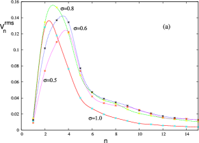
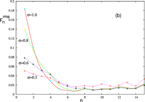
Figure 1: (a) Plots of $v_{n}^{rms}$ for different sizes $\sigma$ (in fm) of initial fluctuations at $\tau=1.98$ fm. Note the net shift in the peak position to smaller values of $n$ with increasing size of initial fluctuations. (b) Plots of initial power spectrum $F_{n}^{rms}$ of spatial anisotropies $F_{n}$. Plots of $F_{n}^{rms}$ in (b) keep rising monotonically with decreasing $n$. However, plots of $v_{n}^{rms}$ in (a) show a drop for low $n$ values.

As we mentioned, the location of first peak in CMBR case directly relates to the size of sound horizon at surface of last scattering. We show in Fig.2, plots of $v_{n}^{rms}$ for different times for one specific simulation (here with initial fluctuation size $\sigma=$ 0.6 fm). Note that there is a consistent shift in the location of first peak towards lower values of $n$ as time increases. If the plasma undergoes freezeout at some specific time $\tau_{fr}$, then the final power spectrum of hadrons will be the one corresponding to the power spectrum shown in Fig.2 at $\tau=\tau_{fr}$. Earlier freezeout (with small values of $\tau_{fr}$) will lead to first peak at larger values of $n$ while the peak will shift to lower $n$ if $\tau_{fr}$ is larger. Thus the location of first peak in the power spectrum of flow fluctuations directly gives information about the freezeout time scale in RHICE.

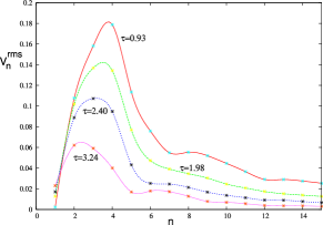
Figure 2: Plots of $v_{n}^{rms}$ at different times $\tau$ (in fm) for one specific simulation (here with initial fluctuation size $\sigma=$ 0.6 fm). Note consistent shift of the location of first peak towards lower values of $n$ as time increases.

We now study the detailed evolution of plots of $v_{n}^{rms}$ in time and focus on the development of acoustic oscillations. It is well known that for elliptic flow the momentum anisotropy starts decreasing after some time (due to decrease in spatial anisotropy in time), but it never reverses sign. This is because the expected oscillation time scale for elliptic flow is too large and radial flow starts dominating before that. It was pointed out in cmbhic that one should expect oscillations to develop fully for shorter wavelength modes, just as for CMBR where modes of short wavelengths undergo several oscillations by the time the largest mode starts entering horizon. Fig. 3 shows the time evolution of $v_{n}^{rms}$ for specific values of $n=7,9,10$, and 11. We note that oscillations develop early for larger values of $n$ (= 10,11) compared to the case for $n=7,9$). Again, this demonstrates the detailed correspondence in the development of acoustic peak structure for flow fluctuations just as in the CMBR case.

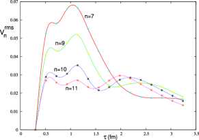
Figure 3: Time evolution of $v_{n}^{rms}$ for specific values of $n$. Note that oscillations develop early for larger values of $n$ (= 10,11) compared to the case for $n=7,9$).

For CMBR case, peaks at larger values of ${\it l}$ correspond to regions which have undergone several oscillations. Similar physics is seen here in Fig.4a which shows varying heights of 1st and 2nd peaks (at the final stage $\tau=3.24$ fm) depending on initial fluctuation size. For CMBR, ratio of second peak to the first peak is directly related to the baryon matter to dark matter ratio. For single fluid component case studied here, we find this ratio to directly relate to the size of the initial fluctuations (with smaller fluctuations having smaller 1st peak to 2nd peak height ratio). Fig.4b shows the plot of this ratio as a function of $\sigma$, the size of initial fluctuations. (More study is needed to see specific dependence of this ratio on $\sigma$.) When one includes aspects of multifluid component nature of QGP, with different particle species interacting with each other, it is entirely possible that a species specific plot of $v_{n}^{rms}$ may encode rich information about different fluid components in terms of ratios of different peak heights.

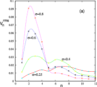
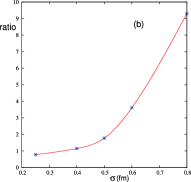
Figure 4: (a) Different plots show varying heights of 1st and 2nd peaks (at the final stage $\tau=3.24$ fm) depending on initial fluctuation size $\sigma$ (in fm). (b) Plot of the ratio of the heights of the 1st peak to the 2nd peak in (a) as a function of $\sigma$

We conclude by emphasizing that our hydrodynamic simulation results have confirmed all the qualitative features predicted in cmbhic for the presence of acoustic peaks in the power spectrum of flow fluctuations just as for CMBR peaks. One important feature remaining is the coherence of fluctuations. Coherence in CMBR case results in pronounced peak structure. However, we have not been able to analyze the nature of dissipation, and contributions of statistical fluctuations in our simulations to a level to comment on whether any possible coherence will be visible in the multiple peak structure of the power spectrum at RHICE. Nonetheless, as mentioned above, the detailed nature of the first peak itself has very rich information about initial fluctuations. A details analysis of the second peak (and other peaks as well) can give immense amount of information about the plasma evolution, including additional constraints on viscosity and equation of state etc. Power spectrum of different particle species (baryons vs. mesons, non-strange vs. strange particles etc.) will give information about interactions between different particle species and their respective contributions to plasma evolution, just as different peak ratios for CMBR give information about baryon to dark matter ratio etc. Another line of deep correspondence with CMBR physics was initiated by us in rhicmag where effects of early stage magnetic fields on power spectrum of flow fluctuations was studies. Magnetohydrodynamics simulations are needed for detailed studies of it. We hope to present such results in future.

We are very grateful to Sanatan Digal for very helpful discussions, especially for simulations. We also thank Partha Bagchi, Arpan Das, Shreyansh S. Dave, Pranati Rath, and Somnath De for useful discussions.

References

- (1) A. P. Mishra, R. K. Mohapatra, P. S. Saumia, and A. M. Srivastava, Phys. Rev. C 77, 064902 (2008); Phys. Rev. C 81, 034903 (2010).
- (2) P. Sorenson, J.Phys. G37 (2010) 094011; B. Alver and G. Roland, Phys. Rev. C 81 (2010) 054905; A. Mocsy and P. Sorenson, Nucl. Phys. A855 (2011) 241, J.I. Kapusta, Nucl. Phys. A862-863 (2011) 47; J.Y. Ollitrault, J. Phys. Conf. Ser. 312 (2011) 012002.
- (3) P. Sorenson, arXiv:0808.0503.
- (4) Steven T. Zalesak, J. Comput. Phys. 31, 335 (1979).
- (5) Michael L. Miller, Klaus Reygers, Sthephen J. Sanders and Peter Steinberg, Ann. Rev. Nucl. Part. Sci. 57, 205 (2007)
- (6) S. Mohapatra, Journal of Physics: Conference Series 389 (2012) 012011; P. Staig and E. Shuryak, J.Phys. G38 (2011) 124039; T. Gorda and P. Romatschke, Phys.Rev. C90 (2014) 5, 054908.
- (7) R. K. Mohapatra, P. S. Saumia, and A. M. Srivastava, Mod. Phys. Lett. A 26, 2477 (2011).