The quench action approach in finite integrable spin chains

Abstract

We consider the problem of constructing the stationary state following a quantum quench, using the exact overlaps for finite size integrable models. We focus on the isotropic Heisenberg spin chain with initial state Néel or Majumdar-Ghosh (dimer), although the proposed approach is valid for an arbitrary integrable model. We consider only eigenstates which do not contain zero-momentum strings because the latter are affected by fictitious singularities that are very difficult to take into account. We show that the fraction of eigenstates that do not contain zero-momentum strings is vanishing in the thermodynamic limit. Consequently, restricting to this part of the Hilbert space leads to vanishing expectation values of local observables. However, it is possible to reconstruct the asymptotic values by properly reweighting the expectations in the considered subspace, at the price of introducing finite-size corrections. We also develop a Monte Carlo sampling of the Hilbert space which allows us to study larger systems. We accurately reconstruct the expectation values of the conserved charges and the root distributions in the stationary state, which turn out to match the exact thermodynamic results. The proposed method can be implemented even in cases in which an analytic thermodynamic solution is not obtainable.

1 Introduction

Understanding the out-of-equilibrium dynamics in isolated quantum many-body systems is one of the most intriguing research topics in contemporary physics, both experimentally [1, 2, 3, 4, 5, 6, 7, 8, 9, 10, 11, 12, 13, 14, 15] and theoretically [16, 17]. The most investigated protocol is that of the quantum quench, in which a system is initially prepared in an eigenstate $|\Psi_{0}\rangle$ of a many-body hamiltonian ${\mathcal{H}}_{0}$. Then a global parameter is suddenly changed, and the system is let to evolve unitarily under a new hamiltonian ${\mathcal{H}}$. There is now compelling evidence that at long times after the quench an equilibrium steady state arises (see for instance Ref. [3]), although its nature is not fully understood yet. In the thermodynamic limit, due to dephasing, it is natural to expect that the equilibrium value of any local observable ${\mathcal{O}}$ is described by the so-called diagonal ensemble as

$$\langle{\mathcal{O}}\rangle_{DE}=\sum\limits_{\lambda}|\langle\Psi_{0}|\lambda\rangle|^{2}\langle\lambda|{\mathcal{O}}|\lambda\rangle,$$ (1)

where the sum is over the eigenstates $|\lambda\rangle$ of the post-quench hamiltonian ${\mathcal{H}}$. Moreover, for generic, i.e., non-integrable, models the Eigenstate Thermalization Hypothesis [18, 19] (ETH) implies that the diagonal ensemble (1) becomes equivalent to the usual Gibbs (thermal) ensemble (a conjecture which has been investigated in many numerical studies [20, 21]).

In integrable models, however, the presence of local or quasi-local integrals of motion strongly affects the dynamics, preventing the onset of thermal behavior. It has been suggested in Ref. [22, 23] that in this situation the post-quench steady-state can be described by the so-called Generalized Gibbs Ensemble ($GGE$) as

$$\langle{\mathcal{O}}\rangle_{GGE}=\frac{1}{Z}\Tr({\mathcal{O}}\rho^{GGE}),\quad\textrm{with}\quad\rho^{GGE}\equiv\frac{1}{Z}\exp\Big{(}-\sum_{j}\beta_{j}Q_{j}\Big{)}.$$ (2)

Here $Q_{j}$ are mutually commuting conserved local (and quasi-local) charges, i.e., $[{\mathcal{H}},Q_{j}]=0\,\forall j$ and $[Q_{j},Q_{k}]=0\,\forall j,k$, whereas $\beta_{j}$ are Lagrange multipliers to be fixed by imposing that $\langle Q_{j}\rangle_{GGE}=\langle\Psi_{0}|Q_{j}|\Psi_{0}\rangle$. This also provides useful sum rules that will be of interest in this paper. The validity of the GGE has been confirmed in non-interacting theories [24, 25, 26, 27, 28, 29, 30, 31, 32, 33, 34, 35, 36, 37], whereas in interacting ones the scenario is still not fully settled and some recent works [38, 39] suggest that the $GGE$ description of the steady state is complete provided that the so-called quasi-local charges [40, 41, 42, 43] are included in the GGE (2).

Valuable insights into this issue have been provided by the so-called quench-action approach [44]. For Bethe ansatz integrable models this method allows one to construct the diagonal ensemble (1) directly in the thermodynamic limit, provided that the overlaps $\langle\lambda|\Psi_{0}\rangle$ are known. The physical idea is that for large system sizes it is possible to approximate the sum over the eigenstates in (1) using a saddle point argument. Specifically, one starts with rewriting (1) as

$$\langle{\mathcal{O}}\rangle_{DE}=\sum\limits_{\lambda}\rho^{DE}\langle\lambda|{\mathcal{O}}|\lambda\rangle,\quad\textrm{with}\quad\rho^{DE}=\exp(-2{\rm Re}({\mathcal{E}}(\lambda))),$$ (3)

where ${\mathcal{E}}(\lambda)\equiv-\ln\langle\lambda|\Psi_{0}\rangle$. For typical initial states $|\Psi_{0}\rangle$, one has ${\mathcal{E}}\propto L$, with $L$ the system size. This reflects the vanishing of the overlaps as $\langle\Psi_{0}|\lambda\rangle\propto e^{-cL}$. As in the standard Thermodynamic Bethe Ansatz (TBA) [45], the extensivity of ${\mathcal{E}}$ suggests that in the thermodynamic limit the sum in (3) is dominated by a saddle point. Remarkably, for some Bethe ansatz solvable models and for simple enough initial states, it is possible to determine this saddle point analytically. This has been done successfully, for instance, for the quench from the Bose-Einstein condensate in the Lieb-Liniger model  [46, 47, 48, 49], for the quench from some product states in the $XXZ$ spin chain [50, 51], for transport in spin chains [52], and for some interacting field theories [53]. The quench action approach allows in principle also to reconstruct the full relaxation dynamics to the steady state [44] as numerically done for the 1D Bose gas [54, 55].

Outline of the results.

In this paper, by combining exact Bethe ansatz and Monte Carlo techniques, we investigate the diagonal ensemble and the quench action approach in finite size integrable models. We consider the spin-$1/2$ XXZ spin-chain with $L$ sites, which is defined by the Hamiltonian

$${\mathcal{H}}\equiv J\sum\limits_{i=1}^{L}\left[\frac{1}{2}(S_{i}^{+}S^{-}_{i+1}+S_{i}^{-}S_{i+1}^{+})+\Delta S_{i}^{z}S_{i+1}^{z}-\frac{1}{4}\right].$$ (4)

Here $S^{\pm}_{i}\equiv(\sigma_{i}^{x}\pm i\sigma_{i}^{y})/2$ are spin operators acting on the site $i$, $S_{i}^{z}\equiv\sigma_{i}^{z}/2$, and $\sigma^{x,y,z}_{i}$ the Pauli matrices. We fix $J=1$ in (4) and use periodic boundary conditions, identifying sites $L+1$ and $1$. The total magnetization $S_{T}^{z}\equiv\sum_{i}S_{i}^{z}=L/2-M$, with $M$ number of down spins (particles), commutes with (4), and it is used to label its eigenstates. The $XXZ$ chain is Bethe ansatz solvable [56, 57] and its eigenstates are in one-to-one correspondence with the solutions of the so-called Bethe equations (see 2.1). The non-equilibrium quench dynamics of the XXZ spin chain has been investigated numerically intensively [58, 59, 60, 61, 62, 63], the GGE with all the local charges has been explicitly constructed [63, 64, 65], and the quench action solution has been provided for some initial states [50, 51].

For concreteness reasons, we focus on the isotropic Heisenberg point ($XXX$), i.e. Hamiltonian (4) with $\Delta=1$, but we stress that our approach applies to arbitrary $\Delta$, and also to arbitrary integrable models. We consider the quenches from the zero-momentum Néel state $|N\rangle$ and the Majumdar-Ghosh state $|MG\rangle$, which are defined as

$$|N\rangle\equiv\Big{(}\frac{|N_{1}\rangle+|N_{2}\rangle}{\sqrt{2}}\Big{)},\qquad|MG\rangle\equiv\Big{(}\frac{|\uparrow\downarrow\rangle-|\downarrow\uparrow\rangle}{\sqrt{2}}\Big{)}^{\otimes L/2}.$$ (5)

Here $|N_{1}\rangle\equiv|\uparrow\downarrow\rangle^{\otimes L/2}$, and $|N_{2}\rangle\equiv|\downarrow\uparrow\rangle^{\otimes L/2}$, with $\otimes$ denoting the tensor product. Note that both $|N\rangle$ and $|MG\rangle$ are invariant under one site translations. Our study relies on the analytical knowledge of the overlaps between the Néel and Majumdar-Ghosh state and the eigenstates of (4) [66, 67, 68, 69, 70, 71].

We first present a detailed overview of the distribution of the overlaps between the initial states and the eigenstates of the model (overlap distribution function). Precisely, we provide numerical results for all the overlaps for finite chains up to $L\leq 38$. Our results are obtained exploiting the analytical formulas presented in Ref. [66] and [69]. Crucially, we restrict ourselves to a truncated Hilbert space, considering only eigenstates of (4) that do not contain zero-momentum strings. Physically, zero-momentum strings correspond to eigenstates amplitudes containing multi-particle bound states having zero propagation velocity. From the Bethe ansatz perspective, in the thermodynamic limit the presence of zero-momentum strings leads to fictitious singularities in the overlap formulas. Dealing with these singularities is a formidable task that requires detailed knowledge of the solutions of the Bethe equations, and it can be done only in very simple cases, e.g., for small chains (as explicitly done for the attractive Lieb-Liniger gas for small number of particles [72]). On the other hand, it has been argued that zero-momentum strings are irrelevant for the reconstruction of the representative state in the thermodynamic limit [51].

For a finite chain, we find that for both the Néel and the Majumdar-Ghosh initial states, the fraction of eigenstates that do not contain zero-momentum strings is vanishing in the thermodynamic limit, meaning that for finite large-enough systems the vast majority of the eigenstates contain zero momentum strings. Specifically, the total number of eigenstates without zero-momentum strings is given in terms of the chain size $L$ by simple combinatorial formulas that we provide. We investigate the effect of the Hilbert space truncation on the diagonal ensemble focusing on the sum rules $\langle Q_{j}\rangle_{DE}=\langle\Psi_{0}|Q_{j}|\Psi_{0}\rangle$ for the conserved quantities $Q_{j}$. We numerically demonstrate that truncating the diagonal ensemble to eigenstates with no zero-momentum strings leads to striking violations of the sum rules, as one would naively expect since most of the states with non zero overlaps have not been included. Precisely, we numerically observe that the truncated diagonal ensemble average $\langle Q_{j}\rangle$ vanish in the thermodynamic limit reflecting the vanishing behavior of the fraction of eigenstates with finite-momentum strings. Thus, for finite chains, eigenstates corresponding to zero-momentum strings cannot be trivially neglected when considering diagonal ensemble averages.

However, this does not imply that the diagonal ensemble cannot be reconstructed from the eigenstates without zero-momentum strings and it is not in contrast with the previous quench action results in the thermodynamic limit [51, 50]. Indeed, we show that the correct diagonal ensemble sum rules can be recovered in the thermodynamic limit by appropriately reweighting the contribution of the finite-momentum strings eigenstates.

We also develop a Monte Carlo scheme, which is a generalization of the approach presented in Ref. [73] to simulate the Generalize Gibbs Ensemble. The method is based on the knowledge of the Néel overlaps $\langle\lambda|N\rangle$ and on the knowledge of the Hilbert space structure of the $XXX$ chain in the Bethe ansatz formalism. The approach allows us to simulate effectively chain with $L\lesssim 60$, although larger systems sizes can in principle be reached.

Strikingly, after the reweighting, although for small chains violations of the conserved quantities sum rules are present, these violations vanish in the thermodynamic limit and the sum rules are restored. This implies that the only effect of the Hilbert space truncation is to introduce finite size scaling corrections. In the quench action language, this means that the eigenstates corresponding to non zero-momentum strings contain enough physical information about the saddle point. This is numerically confirmed by extracting the so-called saddle point root distributions, which in the Bethe ansatz language fully characterize the diagonal ensemble averages in the thermodynamic limit. In the numerical approach these are obtained from the histograms of the Bethe ansatz solutions sampled during the Monte Carlo. Apart from finite size scaling corrections, we observe striking agreement with analytical results, at least for the first few root distributions.

2 Bethe ansatz solution of the Heisenberg ($XXX$) spin chain

In this section we review some Bethe ansatz results for the spin-$\frac{1}{2}$ Heisenberg ($XXX$) chain. Specifically, in subsection 2.1 we discuss the structure of its eigenstates (Bethe states) and the associated Bethe equations. Subsection 2.2 focuses on the string hypothesis and the so-called Bethe-Gaudin-Takahashi (BGT) equations. The form of the BGT equations in the thermodynamic limit is discussed in subsection 2.3. In subsection 2.4 we provide some combinatorial formulas for the total number of the so-called parity-invariant eigenstates. The latter are the only eigenstates having non-zero overlap with the Néel and Majumdar-Ghosh states. Finally, in subsection 2.5 we provide the exact formulas for the local conserved charges of the model.

2.1 Bethe equations and wavefunctions

In the Bethe ansatz framework [56, 45] the generic eigenstate of (4) (Bethe state) in the sector with $M$ particles can be written as

$$|\Psi_{M}\rangle=\sum\limits_{1\leq x_{1}<x_{2}<\dots<x_{M}\leq L}A_{M}(x_{1},x_{2},\dots,x_{M})|x_{1},x_{2},\dots,x_{M}\rangle,$$ (6)

where the sum is over the positions $\{x_{i}\}_{i=1}^{M}$ of the particles, and $A_{M}(x_{1},x_{2},\dots,x_{M})$ is the eigenstate amplitude corresponding to the particles being at positions $x_{1},x_{2},\dots,x_{M}$. The amplitude $A_{M}(x_{1},x_{2},\dots,x_{M})$ is given as

$$A_{M}(x_{1},x_{2},\dots,x_{M})\equiv\sum\limits_{\sigma\in S_{M}}\exp\Big{[}i\sum\limits_{j=1}^{M}k_{\sigma_{j}}x_{j}+i\sum\limits_{i<j}\theta_{\sigma_{i},\sigma_{j}}\Big{]},$$ (7)

where the outermost summation is over the permutations $S_{M}$ of the so-called quasi-momenta $\{k_{\alpha}\}_{\alpha=1}^{M}$. The two-particle scattering phases $\theta_{\alpha,\beta}$ are defined as

$$\theta_{\alpha,\beta}\equiv\frac{1}{2i}\ln\Big{[}-\frac{e^{ik_{\alpha}+ik_{\beta}}-2e^{ik_{\alpha}}+1}{e^{ik_{\alpha}+ik_{\beta}}-2e^{ik_{\beta}}+1}\Big{]}.$$ (8)

The eigenenergy associated with the eigenstate (6) is

$$E=\sum\limits_{\alpha=1}^{M}(\cos(k_{\alpha})-1).$$ (9)

The quasi-momenta $k_{\alpha}$ are obtained by solving the so-called Bethe equations [56]

$$e^{ik_{\alpha}L}=\prod\limits^{M}_{\beta\neq\alpha}\Big{[}-\frac{1-2e^{ik_{\alpha}}-e^{ik_{\alpha}+ik_{\beta}}}{1-2e^{ik_{\beta}}-e^{ik_{\alpha}+ik_{\beta}}}\Big{]}.$$ (10)

It is useful to introduce the rapidities $\{\lambda_{\alpha}\}_{\alpha=1}^{M}$ as

$$k_{\alpha}=\pi-2\arctan(\lambda_{\alpha})\quad\mbox{mod}\,2\pi.$$ (11)

Taking the logarithm on both sides in (10) and using (11), one obtains the Bethe equations in logarithmic form as

$$\arctan(\lambda_{\alpha})=\frac{\pi}{L}J_{\alpha}+\frac{1}{L}\sum\limits_{\beta\neq\alpha}\arctan\Big{(}\frac{\lambda_{\alpha}-\lambda_{\beta}}{2}\Big{)},$$ (12)

where $-L/2<J_{\alpha}\leq L/2$ are the so-called Bethe quantum numbers. It can be shown that $J_{\alpha}$ is half-integer(integer) for $L-M$ even(odd) [45].

Importantly, the $M$-particle Bethe states (6) corresponding to finite rapidities are eigenstates with maximum allowed magnetization (highest-weight eigenstates) $S_{T}^{z}=L/2-M=S_{T}$, with $S_{T}$ the total spin. Due to the $SU(2)$ invariance of (4), all the states in the same $S_{T}$ multiplet and with different $-S_{T}\leq S_{T}^{z}\leq S_{T}$ are eigenstates of the $XXX$ chain, with the same energy eigenvalue. These eigenstates (descendants) are obtained by multiple applications of the total-spin lowering operator $S_{T}^{-}\equiv\sum_{i}S_{i}^{-}$ onto the highest-weight states. In the Bethe ansatz framework, given a highest-weight eigenstate with $M^{\prime}$ particles (i.e., $M^{\prime}$ finite rapidities), its descendants are obtained by supplementing the $M^{\prime}$ rapidities with infinite ones. We anticipate that descendant eigenstates are important here since they have non-zero overlap with the Néel state (cf. section 3).

2.2 String hypothesis & the Bethe-Gaudin-Takahashi (BGT) equations

In the thermodynamic limit $L\to\infty$ the solutions of the Bethe equations (10) form particular “string” patterns in the complex plane, (string hypothesis) [56, 45]. Specifically, the rapidities forming a “string” of length $1\leq n\leq M$ (that we defined here as $n$-string) can be parametrized as

$$\lambda^{j}_{n;\gamma}=\lambda_{n;\gamma}-i(n-1-2j)+i\delta_{n;\gamma}^{j},\qquad j=0,1,\dots,n-1,$$ (13)

with $\lambda_{n;\gamma}$ being the real part of the string (string center), $\gamma$ labelling strings with different centers, and $j$ labelling the different components of the string. In (13) $\delta_{n;\gamma}^{j}$ are the string deviations, which typically, i.e., for most of the chain eigenstates, vanish exponentially with $L$ in the thermodynamic limit. A notable execption are the zero-momentum strings for which string devitions exhibit power-law decay. Note that real rapidities correspond to strings of unit length ($1$-strings, i.e., $n=1$ in (13)).

The string centers $\lambda_{n;\gamma}$ are obtained by solving the so-called Bethe-Gaudin-Takahashi equations [45]

$$2L\theta_{n}(\lambda_{n;\gamma})=2\pi I_{n;\gamma}+\sum\limits_{(m,\beta)\neq(n,\gamma)}\Theta_{m,n}(\lambda_{n;\gamma}-\lambda_{m;\beta}).$$ (14)

Here the generalized scattering phases $\Theta_{m,n}(x)$ read

$$\Theta_{m,n}(x)\equiv\left\{\begin{array}[]{cc}\theta_{|n-m|}(x)+\!\!\!\!\!\sum\limits_{r=1}^{(n+m-|n-m|-1)/2}\!\!\!\!\!2\theta_{|n-m|+2r}(x)+\theta_{n+m}(x)&\quad\mbox{if}\quad n\neq m\\ \sum\limits_{r=1}^{n-1}2\theta_{2r}(x)+\theta_{2n}(x)&\quad\mbox{if}\quad n=m\end{array}\right.$$ (17)

with $\theta_{\alpha}(x)\equiv 2\arctan(x/\alpha)$, and $I_{n;\gamma}$ the Bethe-Takahashi quantum numbers associated with $\lambda_{n;\gamma}$. The solutions of (14), and the Bethe states (6) thereof, are naturally classified according to their “string content” ${\mathcal{S}}\equiv\{s_{n}\}_{n=1}^{M}$, with $s_{n}$ the number of $n$-strings. Clearly, the constraint $\sum_{n=1}^{M}ns_{n}=M$ has to be satisfied. It can be shown that the BGT quantum numbers $I_{n;\gamma}$ associated with the $n$-strings are integers and half-integers for $L-s_{n}$ odd and even, respectively. Moreover, an upper bound for $I_{n;\gamma}$ can be derived as [45]

$$|I_{n;\gamma}|\leq I^{(MAX)}_{n}\equiv\frac{1}{2}(L-1-\sum\limits_{m=1}^{M}t_{m,n}s_{m}),$$ (18)

where $t_{m,n}\equiv 2\mbox{min}(n,m)-\delta_{m,n}$. Using the string hypothesis (13) the Bethe states energy eigenvalue (9) becomes

$$E=-\sum_{n,\gamma}\frac{2n}{\lambda_{n;\gamma}^{2}+n^{2}}.$$ (19)

2.3 The Thermodynamic Bethe Ansatz

In the thermodynamic limit $L\to\infty$ at fixed finite particle density $M/L$ the roots of the BGT equations (14) become dense. One then defines the BGT root distributions for the $n$-strings as $\boldsymbol{\rho}\equiv\{\rho_{n}(\lambda)\}_{n=1}^{\infty}$, with $\rho_{n}(\lambda)\equiv\lim_{L\to\infty}[\lambda_{n;\gamma+1}-\lambda_{n;\gamma}]^{-1}$. Consequently, the BGT equations (14) become an infinite set of coupled non-linear integral equations for the $\rho_{n}(\lambda)$ as

$$a_{n}(\lambda)=\rho_{n}(\lambda)+\rho^{h}_{n}(\lambda)+\sum_{m}(T_{n,m}*\rho_{m})(\lambda),$$ (20)

where $\rho_{n}^{h}(\lambda)$ are the so-called hole-distributions, and the functions $a_{n}(\lambda)$ are defined as

$$a_{n}(x)\equiv\frac{1}{\pi}\frac{n}{x^{2}+n^{2}}.$$ (21)

In (20) $T_{n,m}*\rho_{m}$ denotes the convolution

$$(T_{n,m}*\rho_{m})(\lambda)\equiv\int_{-\infty}^{+\infty}T_{n,m}(\lambda-\lambda^{\prime})\rho_{m}(\lambda^{\prime}),$$ (22)

with the matrix $T_{n,m}(x)\equiv\Theta^{\prime}(x)$ being defined as

$$T_{m,n}(x)\equiv\left\{\begin{array}[]{cc}a_{|n-m|}(x)+\!\!\!\!\!\sum\limits_{r=1}^{(n+m-|n-m|-1)/2}\!\!\!\!\!2a_{|n-m|+2r}(x)+a_{n+m}(x)&\quad\mbox{if}\quad n\neq m\\ \sum\limits_{r=1}^{n-1}2a_{2r}(x)+a_{2n}(x)&\quad\mbox{if}\quad n=m\end{array}\right.$$ (25)

Given a generic, smooth enough, observable ${\mathcal{O}}$, in thermodynamic limit its eigenstate expectation value is replaced by a functional of the root densities $\boldsymbol{\rho}$ as $\langle\boldsymbol{\rho}|{\mathcal{O}}|\boldsymbol{\rho}\rangle$. Moreover, for all the local observables ${\mathcal{O}}$ (the ones considered here) the contribution of the different type of strings factorize, and $\langle\boldsymbol{\rho}|{\mathcal{O}}|\boldsymbol{\rho}\rangle$ becomes

$$\langle\boldsymbol{\rho}|{\mathcal{O}}|\boldsymbol{\rho}\rangle=\sum_{n=1}^{\infty}\int_{-\infty}^{+\infty}d\lambda\rho_{n}(\lambda){\mathcal{O}}_{n}(\lambda),$$ (26)

with ${\mathcal{O}}_{n}(\lambda)$ the $n$-string contribution to the expectation value of ${\mathcal{O}}$.

2.4 Parity-invariant eigenstates with non-zero Néel and Majumdar-Ghosh overlap: counting and string content

Here we provide some exact combinatorial formulas for the total number of parity-invariant eigenstates of the $XXX$ chain in the sector with $L/2$ particles. These are the only eigenstates having, in principle, non-zero overlap with the Néel state and the Majumdar-Ghosh state [66]. Parity-invariant eigenstates correspond to solutions of the Bethe equations containing only pairs of rapidities with opposite sign. In turn, these eigenstates are in one-to-one correspondence with parity-invariant BGT quantum number configurations.

For simplicity we restrict ourselves to the situation with $L$ divisible by four. The strategy of the proof is the same as that used to count the number of solutions of the Bethe-Gaudin-Takahashi equations (see for instance Ref. [74]). Specifically, the idea is to count all the possible BGT quantum numbers configurations corresponding to parity-invariant eigenstates (cf. section 2.2).

We anticipate that the total number of parity-invariant eigenstates $Z_{Neel}$ for a chain of length $L$ is given as

$$Z_{Neel}=2^{\frac{L}{2}-1}+\frac{1}{2}B\Big{(}\frac{L}{2},\frac{L}{4}\Big{)}+1,$$ (27)

with $B(x,y)\equiv x!/(y!(x-y)!)$ the Newton binomial. On the other hand, after excluding the zero-momentum strings one obtains

$$\widetilde{Z}_{Neel}=B\Big{(}\frac{L}{2},\frac{L}{4}\Big{)}.$$ (28)

Note that (27) is only an upper bound for the number of eigenstates with non-zero Néel overlap, while (28) is exact. Before proceeding, we should stress that since the Néel state is not $SU(2)$ invariant, eigenstates with non-zero Néel overlap can contain infinite rapidities. Thus, one has to consider all the possible sectors with $L/2=\ell+N_{\infty}$, and $\ell$ ($N_{\infty}$) the number of finite (infinite) rapidities. Notice that this is different for the Majumdar-Ghosh state, for which only the parity-invariant eigenstates in the sector with $\ell=L/2$ have to be considered (see below).

2.4.1 Parity-invariant states with $\ell$ finite rapidities.

Let us first consider the eigenstate sector with fixed number of finite rapidities $\ell$, the remaining $L/2-\ell$ ones being infinite (see section 2.1). Let us denote the associate string content as ${\mathcal{S}}=\{s_{1},s_{2},\dots,s_{\ell}\}$. Here $s_{n}$ is the number of $n$-strings, with the constraint $\sum_{k}ks_{k}=\ell$. It is straightforward to check that the total number of parity-invariant quantum number pairs ${\mathcal{N}}_{n}(L,{\mathcal{S}})$ in the $n$-string sector is given as

$${\mathcal{N}}_{n}(L,{\mathcal{S}})=\Big{\lfloor}\frac{L}{2}-\frac{1}{2}\sum_{m=1}^{\ell}t_{nm}s_{m}\Big{\rfloor},$$ (29)

where $t_{nm}\equiv 2\textrm{Min}(n,m)-\delta_{n,m}$. Thus, the number of parity-invariant eigenstates of the $XXX$ chain ${\mathcal{N}}(L,{\mathcal{S}})$ compatible with string content ${\mathcal{S}}$ is obtained by choosing in all the possible ways the associated parity-invariant quantum number pairs as

$${\mathcal{N}}(L,{\mathcal{S}})=\prod_{m=1}^{\ell}B\left({\mathcal{N}}_{m},\left\lfloor\frac{s_{m}}{2}\right\rfloor\right).$$ (30)

Here the product is because each string sector is treated independently, while the factor $1/2$ in $s_{m}/2$ is because since all quantum numbers are organized in pairs, only half of them have to be specified. Note that in each $n$-string sector only one zero momentum (i.e., zero quantum number) string is allowed, due to the fact that repeated solutions of the BGT equation are discarded. Moreover, from (29) one has that $s_{m}$ is odd (even) only if this zero momentum string is (not) present.

We now proceed to consider the string configurations with fixed particle number $\ell\leq L/2$ and fixed number of strings $1\leq q\leq\ell$. Note that due to parity invariance $\ell$ must be even. Also, in determining $q$ strings of different length are treated equally, i.e., $q=\sum_{m}s_{m}$. For a given fixed pair $\ell,q$ the total number of allowed quantum number configurations by definition is given as

$${\mathcal{N}}^{\prime}(L,\ell,q)=\sum\limits_{\{\{s_{m}\}\,:\,\sum ms_{m}=\ell,\sum s_{m}=q\}}{\mathcal{N}}(L,{\mathcal{S}}),$$ (31)

where the sum is over the string content $\{s_{m}\}_{m=1}^{\ell}$ compatible with the constraints $\sum_{m}s_{m}=q$ and $\sum_{m}ms_{m}=\ell$. The strategy now is to write a recursive relation in both $\ell,q$ for ${\mathcal{N}}^{\prime}(L,\ell,q)$. It is useful to consider a shifted string content ${\mathcal{S}}^{\prime}$ defined as

$${\mathcal{S}}^{\prime}\equiv\{s_{m+1}\}\quad\textrm{with}\,s_{m}\in{\mathcal{S}},\,\forall m.$$ (32)

Using the definition of $t_{ij}$, it is straightforward to derive that

$$t_{ij}=t_{i-1,j-1}+2,$$ (33)

which implies that ${\mathcal{N}}_{n}(L,{\mathcal{S}})$ (see (29)) satisfies the recursive equation

$${\mathcal{N}}_{n}(L,{\mathcal{S}})={\mathcal{N}}_{n-1}(L-2q,{\mathcal{S}}^{\prime}).$$ (34)

After substituting (34) in (30) one obtains

$${\mathcal{N}}(L,{\mathcal{S}})=B\Big{(}{\mathcal{N}}_{1}(L,{\mathcal{S}}),\Big{\lfloor}\frac{s_{1}}{2}\Big{\rfloor}\Big{)}{\mathcal{N}}(L-2q,{\mathcal{S}}^{\prime}).$$ (35)

Finally, using (35) in (31), one obtains a recursive relation for ${\mathcal{N}}^{\prime}(L,\ell,q)$ as

$${\mathcal{N}}^{\prime}(L,\ell,q)=\sum_{s=0}^{q-1}B\Big{(}\frac{L}{2}-q+\Big{\lfloor}\frac{s}{2}\Big{\rfloor},\left\lfloor\frac{s}{2}\right\rfloor\Big{)}{\mathcal{N}}^{\prime}\left(L-2q,\ell-q,q-s\right),$$ (36)

with the condition that for $\ell=q$ one has

$${\mathcal{N}}^{\prime}(L,q,q)=B\Big{(}\Big{\lfloor}\frac{L-q}{2}\Big{\rfloor},\Big{\lfloor}\frac{q}{2}\Big{\rfloor}\Big{)}.$$ (37)

This is obtained by observing that if $\ell=q$ only $1$-strings are allowed and (29) gives ${\mathcal{N}}_{n}(L,{\mathcal{S}})=\lfloor(L-q)/2\rfloor$. It is straightforward to check that to satisfy (36) for $q$ even one has to choose

$${\mathcal{N}}^{\prime}(L,\ell,q)=\frac{q}{\ell}B\Big{(}\frac{L-\ell}{2},\frac{q}{2}\Big{)}B\Big{(}\frac{\ell}{2},\frac{q}{2}\Big{)},$$ (38)

Instead, for $q$ odd one has

$${\mathcal{N}}^{\prime}(L,\ell,q)=\frac{\ell-q+1}{\ell}B\Big{(}\frac{L-\ell}{2},\frac{q-1}{2}\Big{)}B\Big{(}\frac{\ell}{2},\frac{q-1}{2}\Big{)}.$$ (39)

The number of eigenstates in the sector with $\ell$ particles having nonzero Néel overlap $Z^{\prime}_{Neel}(L,\ell)$ is obtained from (38) and (39) by summing over all possible values of $q$ as

$$Z^{\prime}_{Neel}(L,\ell)=\sum\limits_{q=1}^{\ell}{\mathcal{N}}^{\prime}(L,\ell,q).$$ (40)

It is convenient to split the summation in (40) considering odd and even $q$ separately. For $q$ odd one obtains

$$\sum\limits_{k=0}^{\ell/2-1}{\mathcal{N}}^{\prime}(L,\ell,2k+1)=B\Big{(}\frac{L}{2}-1,\frac{\ell}{2}-1\Big{)},$$ (41)

while for $q$ even one has

$$\sum\limits_{k=0}^{\ell/2}{\mathcal{N}}^{\prime}(L,\ell,2k)=B\Big{(}\frac{L}{2}-1,\frac{\ell}{2}\Big{)}.$$ (42)

Putting everything together one obtains

$$Z^{\prime}_{Neel}(L,\ell)=B\Big{(}\frac{L}{2}-1,\frac{\ell}{2}-1\Big{)}+B\Big{(}\frac{L}{2}-1,\frac{\ell}{2}\Big{)}.$$ (43)

The total number of eigenstates with nonzero Néel overlap $Z_{Neel}(L)$ (cf. (27)) is obtained from (43) by summing over the allowed values of $\ell=2k$ with $k=0,1,\dots,L/2$. Note that the sum is over $\ell$ even due to the parity invariance.

Finally, it is interesting to observe that the total number $Z_{MG}$ of parity-invariant eigenstates having non zero overlap with the Majumdar-Ghosh state is obtained from Eq (43) by replacing $\ell=L/2$, to obtain

$$Z_{MG}=B\Big{(}\frac{L}{2}-1,\frac{L}{4}-1\Big{)}+B\Big{(}\frac{L}{2}-1,\frac{L}{4}\Big{)}.$$ (44)

Physically, this is due to the fact that the Majumdar-Ghosh state is invariant under $SU(2)$ rotations, implying that only eigenstates with zero total spin $S=0$ can have non-zero overlap.

2.4.2 Excluding the zero-momentum strings.

One should first observe that for the generic eigenstate of the $XXX$ chain with $\ell$ finite rapidities, due to parity invariance and the exclusion of zero-momentum strings, only $n$-strings with length $n\leq\ell/2$ are allowed. Also, the string content can be written as ${\mathcal{S}}\equiv\{s_{1},\dots,s_{\ell/2}\}$, i.e., $s_{m}=0$ $\forall m>\ell/2$. Due to the parity invariance one has that $s_{m}$ is always even. Clearly one has $\sum_{m=1}^{\ell/2}ms_{m}=\ell$. Finally, the total number of parity-invariant quantum numbers $\widetilde{\mathcal{N}}_{n}$ in the $n$-string sector is given as

$$\widetilde{\mathcal{N}}_{n}(L,{\mathcal{S}})=\frac{L}{2}-\frac{1}{2}\sum_{m=1}^{\ell/2}t_{nm}s_{m}.$$ (45)

The proof now proceeds as in the previous section. One defines the total number of eigenstates with nonzero Néel overlap in the sector with fixed $\ell$ finite rapidities and $q$ different string types as $\widetilde{\mathcal{N}}^{\prime}(L,\ell,q)$. It is straightforward to show that $\widetilde{\mathcal{N}}^{\prime}(L,\ell,q)$ obeys the recursive relation

$$\widetilde{\mathcal{N}}^{\prime}(L,\ell,q)=\sum_{s=0}^{q/2-1}B\Big{(}\frac{L}{2}-q+s,s\Big{)}\widetilde{\mathcal{N}}^{\prime}\Big{(}L-2q,\frac{\ell-q}{2},\frac{q}{2}-s\Big{)},$$ (46)

with the constraint

$$\widetilde{\mathcal{N}}^{\prime}(L,1,1)=\frac{L}{2}-1.$$ (47)

The solution of (46) is given as

$$\widetilde{\mathcal{N}}^{\prime}(L,\ell,q)=\frac{L-2\ell+2}{L-\ell+2}B\Big{(}\frac{L-\ell}{2}+1,q\Big{)}B\Big{(}\frac{\ell}{2}-1,\frac{q}{2}-1\Big{)}.$$ (48)

After summing over the allowed values of $q=2k$ with $k=1,2,\dots,\ell/2$ one obtains the total number of eigenstates with nonzero Néel overlap at fixed number of particles $\ell$ $\widetilde{Z}_{Neel}^{\prime}(L,\ell)$ as

$$\widetilde{Z}_{Neel}^{\prime}(L,\ell)=B\Big{(}\frac{L}{2},\frac{\ell}{2}\Big{)}-B\Big{(}\frac{L}{2},\frac{\ell}{2}-1\Big{)}.$$ (49)

by summing over $\ell$ one obtains (28). Similar to (44) the total number of eigenstates $\widetilde{Z}_{MG}$ having non-zero overlap with the Majumdar-Ghosh state is obtained from (49) by replacing $\ell\to L/2$, to obtain

$$\widetilde{Z}_{MG}=B\Big{(}\frac{L}{2},\frac{L}{4}\Big{)}-B\Big{(}\frac{L}{2},\frac{L}{4}-1\Big{)}.$$ (50)

Interestingly, using (44) and (50), one obtains that the ratio $\widetilde{Z}_{MG}/Z_{MG}$ is given as

$$\frac{\widetilde{Z}_{MG}}{Z_{MG}}=\frac{4}{4+L}.$$ (51)

2.5 The conserved charges

The $XXX$ chain exhibits an extensive number of mutually commuting local conserved charges [75] $Q_{n}$ ($n\in\mathbb{N}$), i.e.,

$$[Q_{n},{\mathcal{H}}]=0\quad\forall n\quad\textrm{and}\quad[Q_{n},Q_{m}]=0\quad\forall n,m.$$ (52)

The corresponding charges eigenvalues are given as

$$\left.Q_{n+1}\equiv\frac{i}{(n-1)!}\frac{d^{n}}{dy^{n}}\ln\tau(y)\right|_{y=i},$$ (53)

where $y$ is a spectral parameter and $\tau(y)$ is the eigenvalue of the so-called transfer matrix in the Algebraic Bethe Ansatz framework [57]. The analytic expression for $\tau(y)$ in terms of the solutions $\{\lambda_{\alpha}\}$ of the Bethe equations (10) is given as

$$\tau(y)\equiv\Big{(}\frac{y+i}{2}\Big{)}^{L}\prod\limits_{\alpha}\frac{y-\lambda_{\alpha}-2i}{y-\lambda_{\alpha}}+\Big{(}\frac{y-i}{2}\Big{)}^{L}\prod\limits_{\alpha}\frac{y-\lambda_{\alpha}+2i}{y-\lambda_{\alpha}}.$$ (54)

Interestingly, one can check that the second term in (54) does not contribute to $Q_{n}$, at least for small enough $n\ll L$. For a generic Bethe state, using the string hypothesis (13) the eigenvalue of $Q_{n}$ is obtained by summing independently the contributions of the BGT roots (see (14)) as

$$Q_{n}=\sum_{k,\gamma}g_{n,k}(\lambda_{k;\gamma}).$$ (55)

Using the string hypothesis (cf. (13)) and (53) (54), one obtains the first few functions $g_{n,k}$ in terms of the solutions of the BGT equations (14) as

$$g_{2,k}=-\frac{2k}{\lambda^{2}_{k;\gamma}+k^{2}}, \quad g_{3,k}=-\frac{4k\lambda_{k;\gamma}}{(\lambda_{k;\gamma}^{2}+k^{2})^{2}}$$ (56)

$$g_{4,k}=\frac{2k(k^{2}-3\lambda_{k;\gamma}^{2})}{(k^{2}+\lambda_{k;\gamma}^{2})^{3}}, \quad g_{5,k}=\frac{8k\lambda_{k;\gamma}(k^{2}-\lambda_{k;\gamma}^{2})}{(k^{2}+\lambda_{k;\gamma}^{2})^{4}}$$

$$g_{6,k}=-\frac{2k(5\lambda_{k;\gamma}^{4}-10k^{2}\lambda_{k;\gamma}^{2}+k^{4})}{(k^{2}+\lambda_{k;\gamma}^{2})^{5}}.$$

It is interesting to observe that $g_{n,k}$ is vanishing in the limit $\lambda_{k;\gamma}\to\infty$. This is expected to hold for the generic $n,k$, and it is a consequence of the $SU(2)$ invariance of the conserved charges. Finally, in the thermodynamic limit $L\to\infty$ one can replace the sum over $\gamma$ in (55) with an integral to obtain

$$q_{n}\to\sum_{k=1}^{\infty}\int_{-\infty}^{+\infty}d\lambda\rho_{k}(\lambda)g_{n,k}(\lambda),$$ (57)

where the BGT root distributions $\rho_{k}(\lambda)$ are solutions of the system of integral equations (20).

3 Overlap between the Bethe states and some simple product states

Here we detail the Bethe ansatz results for the overlap of the Bethe states (cf. (6)) with the zero-momentum (one-site shift invariant) Néel state $|N\rangle$ and the Majumdar-Ghosh (MG) $|MG\rangle$ state (cf. (5)). In particular, we specialize the Bethe ansatz results to the case of eigenstates described by perfect strings.

3.1 Néel state overlaps

We start discussing the overlaps with the Néel state. As shown in Ref. [66, 51], only parity-invariant Bethe states have non-zero overlap with the Néel state. The corresponding solutions of the Bethe equations (10) contain only pairs of rapidities with opposite sign. Here we denote the generic parity-invariant rapidity configuration as $|\{\pm\tilde{\lambda}_{j}\}_{j=1}^{m},n_{\infty}\rangle$, i.e., considering only positive rapidities (as stressed by the tilde in $\tilde{\lambda}_{j}$). Here $m$ is the number of rapidity pairs. Since the Néel state is not invariant under $SU(2)$ rotations, eigenstates with infinite rapidities can have non-zero Néel overlaps. We denote the number of infinite rapidities as $N_{\infty}$. Note that one has $M=L/2=N_{\infty}+2m$. The density of infinite rapidities is denoted as $n_{\infty}\equiv N_{\infty}/L$. The overlap between the Bethe states and the Néel state $|N\rangle$ reads [51, 69]

$$\frac{\langle N|\{\pm\tilde{\lambda}_{j}\}_{j=1}^{m},n_{\infty}\rangle}{|||\{\tilde{\lambda}_{j}\}_{j=1}^{m},n_{\infty}\rangle||}=\frac{\sqrt{2}N_{\infty}!}{\sqrt{(2N_{\infty})!}}\left[\prod_{j=1}^{m}\frac{\sqrt{\tilde{\lambda}_{j}^{2}+1}}{4\tilde{\lambda}_{j}}\right]\sqrt{\frac{\textrm{det}_{m}(G^{+})}{\textrm{det}_{m}(G^{-})}}.$$ (58)

The matrix $G^{\pm}$ is defined as

$$\quad G^{\pm}_{jk}=\delta_{jk}\Big{(}LK_{1/2}(\tilde{\lambda}_{j})-\sum\limits_{l=1}^{m}K_{1}^{+}(\tilde{\lambda}_{j},\tilde{\lambda}_{l})\Big{)}+K_{1}^{\pm}(\tilde{\lambda}_{j},\tilde{\lambda}_{k}),\quad\,j,k=1,\dots,m,$$ (59)

where

$$K_{1}^{\pm}(\lambda,\mu)=K_{1}(\lambda-\mu)\pm K_{1}(\lambda+\mu)\quad\textrm{with}\quad K_{\alpha}(\lambda)\equiv\frac{8\alpha}{\lambda^{2}+4\alpha^{2}}.$$ (60)

Note that our definitions of $K_{\alpha}(\lambda)$ differs from the one in Ref. [66], due to a factor $2$ in the definition of the rapidities (cf. (13)).

3.2 The string hypothesis: Reduced formulas for the Néel overlaps

Here we consider the overlap formula for the Néel state (58) in the limit $L\to\infty$, assuming that the rapidities form perfect strings, i.e., $\delta_{n;\gamma}^{j}=0$ in (13). Then it is possible to rewrite (58) in terms of the string centers $\tilde{\lambda}_{n;\alpha}$ only. We restrict ourselves to parity-invariant rapidity configurations with no zero-momentum strings, i.e., with finite string centers (cf. (13)). We denote the generic parity-invariant string configuration as $\{\tilde{\lambda}_{n;\gamma}\}$, where $\gamma$ labels the different non-zero string centers, and $n$ is the string length. Note that due to parity invariance and the exclusion of zero-momentum strings, only strings of length up to $m$ are allowed. The string content (cf. 2.2) of parity-invariant Bethe states is denoted as $\widetilde{\mathcal{S}}=\{\tilde{s}_{1},\dots,\tilde{s}_{m}\}$, with $\tilde{s}_{n}$ the number of pairs of $n$-strings.

It is convenient to split the indices $i,j$ in $G^{\pm}_{ij}$ (cf. (59)) as $i=(n,\gamma,i)$ and $j=(m,\gamma^{\prime},j)$, with $n,m$ being the length of the strings, $\gamma,\gamma^{\prime}$ labelling the corresponding string centers, and $i,j$ the components of the two strings. Using (59) and (60), one has that for two consecutive rapidities in the same string, i.e., for $m=n,\gamma=\gamma^{\prime},|i-j|=2$, the matrices $G^{\pm}_{jk}$ become ill-defined in the thermodynamic limit. Precisely, $K_{1}(\tilde{\lambda}_{n;\gamma}^{i}-\tilde{\lambda}_{n;\gamma}^{i+1})\sim 1/(\delta_{n;\gamma}^{i}-\delta_{n;\gamma}^{i+1})$, implying that $G_{ij}^{\pm}$ diverges in the thermodynamic limit. However, as the same type of divergence occurs in both $G^{+}$ and $G^{-}$, their ratio (cf. (58)) is finite.

The finite part of the ratio $\det G^{+}/\det G^{-}$ can be extracted using the same strategy as in Ref. [76, 77] (see also Ref. [66, 72]). One obtains that $\det G^{+}/\det G^{-}\to\det\widetilde{G}^{+}/\det\widetilde{G}^{-}$. The reduced matrix $\widetilde{G}^{+}$ depends only on the indices $(n,\gamma)$ and $(m,\gamma^{\prime})$ of the “string center” and it is given as

$$\frac{1}{2}\widetilde{G}^{+}_{(n,\gamma)(m,\gamma^{\prime})}=\left\{\begin{array}[]{cc}L\theta_{n}^{\prime}(\tilde{\lambda}_{n;\gamma})-\sum\limits_{(\ell,\alpha)\neq(n,\gamma)}\Big{[}\Theta^{\prime}_{n,\ell}(\tilde{\lambda}_{n;\gamma}-\tilde{\lambda}_{\ell;\alpha})&\quad\textrm{if}\,(n,\gamma)=(m,\gamma^{\prime})\\ +\Theta^{\prime}_{n,\ell}(\tilde{\lambda}_{n;\gamma}+\tilde{\lambda}_{\ell;\alpha})\Big{]}&\\ \\ \Theta^{\prime}_{n,m}(\tilde{\lambda}_{n;\gamma}-\tilde{\lambda}_{m;\gamma^{\prime}})+\Theta^{\prime}_{n,m}(\tilde{\lambda}_{n;\gamma}+\tilde{\lambda}_{m;\gamma^{\prime}})&\quad\textrm{if}\,(n,\gamma)\neq(m,\gamma^{\prime})\end{array}\right.$$ (61)

Here $\theta_{n}^{\prime}(x)\equiv d\theta_{n}(x)/dx=2n/(n^{2}+x^{2})$ and $\Theta^{\prime}(x)\equiv d\Theta(x)/dx$, with $\Theta(x)$ as defined in (17). Similarly, for $\widetilde{G}^{-}$ one obtains

$$\frac{1}{2}\widetilde{G}^{-}_{(n,\gamma)(m,\gamma^{\prime})}=\left\{\begin{array}[]{cc}(L-1)\theta^{\prime}_{n}(\tilde{\lambda}_{n;\gamma})-2\sum\limits_{k=1}^{n-1}\theta^{\prime}_{k}(\tilde{\lambda}_{n;\gamma})&\textrm{if}\,(n,\gamma)=(m,\gamma^{\prime})\\ -\sum\limits_{(\ell,\alpha)\neq(n,\gamma)}\Big{[}\Theta^{\prime}_{n,\ell}(\tilde{\lambda}_{n;\gamma}-\tilde{\lambda}_{\ell;\alpha})+\Theta^{\prime}_{n,\ell}(\tilde{\lambda}_{n;\gamma}+\tilde{\lambda}_{\ell;\alpha})\Big{]}\\ \\ \Theta^{\prime}_{n,m}(\tilde{\lambda}_{n;\gamma}-\tilde{\lambda}_{m;\gamma^{\prime}})-\Theta^{\prime}_{n,m}(\tilde{\lambda}_{n;\gamma^{\prime}}+\tilde{\lambda}_{m;\gamma^{\prime}}))&\textrm{if}\,(n,\gamma)\neq(m,\gamma^{\prime})\end{array}\right.$$ (62)

We should stress that in presence of zero-momentum strings, additional divergences as $1/(\delta_{n;\gamma}^{i}+\delta_{n;\gamma}^{i+1})$ appear in $\widetilde{G}^{\pm}$, due to the term $K_{1}(\lambda+\mu)$ in (59). The treatment of these divergences is a challenging task because it requires, for each different type of string, the precise knowledge of the string deviations, meaning their dependence on $L$. Some results have been provided for small strings in Ref. [72].

Finally, using the string hypothesis and the parity-invariance condition, the prefactor of the determinant ratio in (58) becomes

$$\quad\prod\limits_{j=1}^{m}\frac{\sqrt{\tilde{\lambda}_{j}^{2}+1}}{4\tilde{\lambda}_{j}}=\frac{1}{4^{m}}\prod\limits_{n=1}^{m}\prod\limits_{\ell=1}^{\tilde{s}_{n}}\left[\frac{\sqrt{n^{2}+\tilde{\lambda}^{2}_{n;\ell}}}{\tilde{\lambda}_{n;\ell}}\prod\limits_{k=0}^{\lceil n/2\rceil-1}\frac{(2k)^{2}+\tilde{\lambda}^{2}_{n;\ell}}{(2k+1)^{2}+\tilde{\lambda}^{2}_{n;\ell}}\right]^{(-1)^{n}},$$ (63)

where $\tilde{s}_{n}$ is the number of $n$-string pairs in the Bethe state.

3.3 Overlap with the Majumdar-Ghosh state

The overlap between a generic eigenstate of the $XXX$ chain $|\{\pm\tilde{\lambda}_{j}\}\rangle$ and the Majumdar-Ghosh state can be obtained from the Néel state overlap (58) as [69]

$$\langle MG|\{\pm\tilde{\lambda}_{j}\}_{j=1}^{m}\rangle=\prod\limits_{j=1}^{m}\frac{1}{2}\Big{(}1-\frac{\tilde{\lambda}_{j}-i}{\tilde{\lambda}_{j}+i}\Big{)}\Big{(}1+\frac{\tilde{\lambda}_{j}+i}{\tilde{\lambda}_{j}-i}\Big{)}\langle N|\{\pm\tilde{\lambda}_{j}\}_{j=1}^{m}\rangle.$$ (64)

Notice that the Bethe states having non-zero overlap with the Majumdar-Ghosh state do not contain infinite rapidities ($N_{\infty}=0$), in contrast with the Néel case (cf. (58)). Using the string hypothesis, the multiplicative factor in (64) is rewritten as

$$\prod\limits_{j=1}^{m}\frac{1}{2}\Big{(}1-\frac{\tilde{\lambda}_{j}-i}{\tilde{\lambda}_{j}+i}\Big{)}\Big{(}1+\frac{\tilde{\lambda}_{j}+i}{\tilde{\lambda}_{j}-i}\Big{)}=$$ (65)

$$\qquad 2^{m}\prod\limits_{n=1}^{m}\prod\limits_{\ell=1}^{\tilde{s}_{n}}\tilde{\lambda}_{n;\ell}^{1+(-1)^{n}}(\tilde{\lambda}^{2}_{n;\ell}+n^{2})\prod\limits_{k=0}^{\lfloor n/2\rfloor}\Big{[}\tilde{\lambda}_{n;\ell}^{2}+\Big{(}2k+\frac{1-(-1)^{n}}{2}\Big{)}^{2}\Big{]}^{-2}.$$

3.4 The Néel overlap in the thermodynamic limit

In the thermodynamic limit $L\to\infty$ the extensive part of the Néel overlap (58) can be written as [66]

$$-\lim_{L\to\infty}\ln\left[\frac{\langle N|\{\pm\tilde{\lambda}_{j}\}_{j=1}^{m},n_{\infty}\rangle}{|||\{\tilde{\lambda}_{j}\}_{j=1}^{m},n_{\infty}\rangle||}\right]=\frac{L}{2}\Big{(}n_{\infty}\ln 2+\sum_{n=1}^{\infty}\int_{0}^{\infty}d\lambda\rho_{n}(\lambda)[g_{n}(\lambda)+2n\ln(4)]\Big{)},$$ (66)

where

$$\quad g_{n}(\lambda)=\sum_{l=1}^{n-1}\Big{[}f_{n-1-2l}(\lambda)-f_{n-2l}(\lambda)\Big{]},\quad\textrm{with}\quad f_{n}(\lambda)=\ln\Big{(}\lambda^{2}+\frac{n^{2}}{4}\Big{)},$$ (67)

and

$$n_{\infty}=1-2\sum_{m=1}^{\infty}m\int_{-\infty}^{\infty}d\lambda\rho_{m}(\lambda).$$ (68)

Note that (66) is extensive, due to the prefactor $L/2$. Also, (66) is obtained only from (63), while the subextensive contributions originating from the determinant ratio $\det_{m}(G^{+})/\det_{m}(G^{-})$ in (58) are neglected. We should mention that (66) acts as a driving term in the quench action formalism (cf. section 4).

4 Quench action treatment of the steady state

The quench action formalism [44] allows one to construct a saddle point approximation for the diagonal ensemble. First, in the thermodynamic limit the sum over the chain eigenstates in (1) can be recast into a functional integral over the BGT root distributions $\boldsymbol{\rho}\equiv\{\rho_{n}(\lambda)\}_{n=1}^{\infty}$ (cf. section 2.3) as

$$\sum\limits_{\alpha}\rightarrow\int{\mathcal{D}}\boldsymbol{\rho}e^{S_{YY}(\boldsymbol{\rho})}.$$ (69)

Here ${\mathcal{D}}\boldsymbol{\rho}\equiv\prod_{n=1}^{\infty}{\mathcal{D}}\rho_{n}(\lambda)$ and $S_{YY}(\boldsymbol{\rho})$ is the Yang-Yang entropy

$$\quad S_{YY}(\boldsymbol{\rho})\equiv L\sum_{n=1}^{\infty}\int_{-\infty}^{+\infty}d\lambda\Big{[}\rho_{n}(\lambda)\ln\Big{(}1+\frac{\rho_{n}^{h}(\lambda)}{\rho_{n}(\lambda)}\Big{)}+\rho_{n}^{h}(\lambda)\ln\Big{(}1+\frac{\rho_{n}(\lambda)}{\rho^{h}_{n}(\lambda)}\Big{)}\Big{]},$$ (70)

which counts the number of microscopic Bethe states (6) leading to the same $\boldsymbol{\rho}$ in the thermodynamic limit. Using (69), the diagonal ensemble expectation value (1) of a generic observable ${\mathcal{O}}$ becomes

$$\quad\langle{\mathcal{O}}\rangle=\int{\mathcal{D}}\boldsymbol{\rho}\exp\Big{[}2\Re\ln\langle\Psi_{0}|\boldsymbol{\rho}\rangle+S_{YY}(\boldsymbol{\rho})\Big{]}\langle\boldsymbol{\rho}|{\mathcal{O}}|\boldsymbol{\rho}\rangle.$$ (71)

Here it is assumed that in the thermodynamic limit the eigenstate expectation values $\langle\alpha|{\mathcal{O}}|\alpha\rangle$ (cf. (1)) become smooth functionals of the root distributions $\boldsymbol{\rho}$, whereas $\langle\boldsymbol{\rho}|\Psi_{0}\rangle$ for the Néel state is readily obtained from (66).

The functional integral in (71) can be evaluated in the limit $L\to\infty$ using the saddle point approximation. One has to minimize the functional ${\mathcal{F}}(\boldsymbol{\rho})$ defined as

$$L{\mathcal{F}}(\boldsymbol{\rho})\equiv 2\Re\ln\langle\boldsymbol{\rho}|\Psi_{0}\rangle+S_{YY}(\boldsymbol{\rho}(\lambda)),$$ (72)

with respect to $\boldsymbol{\rho}$, i.e., solving $\delta{\mathcal{F}}(\boldsymbol{\rho})/\delta\boldsymbol{\rho}|_{\boldsymbol{\rho}=\boldsymbol{\rho^{*}}}=0$, under the constraint that the thermodynamic BGT equations (20) hold. Finally, one obtains from (71) that in the thermodynamic limit

$$\langle{\mathcal{O}}\rangle=\langle\boldsymbol{\rho^{*}}|{\mathcal{O}}|\boldsymbol{\rho^{*}}\rangle.$$ (73)

Remarkably, for the quench with initial state the Néel state $|\Psi_{0}\rangle=|N\rangle$ the saddle point root distributions ${\rho_{n}^{*}(\lambda)}_{n=1}^{\infty}$ can be obtained analytically [66]. The first few are given as

$$\quad\rho^{*}_{1}(\lambda)=\frac{8(4+\lambda^{2})}{\pi(19+3\lambda^{2})(1+6\lambda^{2}+\lambda^{4})},$$ (74)

$$\quad\rho_{2}^{*}(\lambda)=\frac{8\lambda^{2}(9+\lambda^{2})(4+3\lambda^{2})}{\pi(2+\lambda^{2})(16+14\lambda^{2}+\lambda^{4})(256+132\lambda^{2}+9\lambda^{4})},$$ (75)

$$\quad\rho_{3}^{*}(\lambda)=\frac{8(1+\lambda^{2})^{2}(5+\lambda^{2})(16+\lambda^{2})(21+\lambda^{2})}{\pi(19+3\lambda^{2})(9+624\lambda^{2}+262\lambda^{4}+32\lambda^{6}+\lambda^{8})(509+5\lambda^{2}(26+\lambda^{2}))}.$$ (76)

5 The role of the zero-momentum strings Bethe states

In this section we discuss generic features of the overlaps between the eigenstates (Bethe states) of the Heisenberg spin chain and the Néel state. We exploit the Bethe ansatz solution of the chain (see section 2) as well as exact results for the Néel overlaps (see section 3). We focus on finite chains with $L\lesssim 40$ sites. The only Bethe states having non zero Néel overlap are the parity-invariant Bethe states (see section 3). We denote their total number as $Z_{Neel}$. Crucially, here we restrict ourselves to the parity-invariant Bethe states that do not contain zero-momentum strings. We denote the total number of these eigenstates as $\widetilde{Z}_{Neel}$.

Interestingly, the fraction of eigenstates with no zero-momentum strings, i.e., $\widetilde{Z}_{Neel}/Z_{Neel}$, is vanishing as $L^{-1/2}$ in the thermodynamic limit, meaning that zero-momentum strings eigenstates are dominant in number for large chains. This has consequences at the level of the overlap sum rules for the local conservation laws of the model that cannot be saturated by a vanishing fraction of states. Indeed, limiting ourselves to states that do not contain zero momentum strings, we find that all sum rules exhibit vanishing behavior as $L^{-1/2}$ upon increasing the chain size, reflecting the same vanishing behavior as $\widetilde{Z}_{Neel}/Z_{Neel}$. A similar scenario holds for the overlaps with the Majumdar-Ghosh state, where excluding the zero-momentum strings leads to a $1/L$ behavior. This shows that zero-momentum strings eigenstates are not naively negligible.

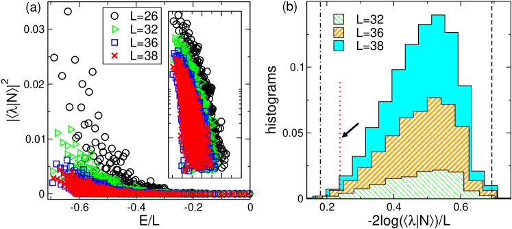
Figure 1: Néel overlaps with the eigenstates of the Heisenberg spin chain: Numerical results obtained from the full scanning of the chain Hilbert space. Eigenstates corresponding to zero-momentum strings are excluded. (a) Squared overlaps $|\langle\lambda|N\rangle|^{2}$ plotted as function of the eigenstates energy density $E/L$. Here $|\lambda\rangle$ denotes the generic eigenstate. The data are for chains with length $26\leq L\leq 38$. The inset highlights the exponential decay as a function of $E/L$ (note the logarithmic scale on the $y$ axis). (b) Overlap distribution function: Histograms of $-2\ln\langle\lambda|N\rangle/L$. The $y$-axis is rescaled by a factor $10^{5}$ for convenience. The dash-dotted and dashed vertical lines are the Néel overlaps with the $XXX$ chain ground state and the ferromagnetic state, respectively. The dotted line (see the arrow) is the result obtained using the quench action approach.

5.1 Néel overlap distribution function: Overview

Here we overview the Bethe ansatz results for the Néel overlaps with the eigenstates of the $XXX$ chain. The total number of parity-invariant eigenstates $Z_{Neel}$ having, in principle, non-zero Néel overlap is given as

$$Z_{Neel}=2^{\frac{L}{2}-1}+\frac{1}{2}B\Big{(}\frac{L}{2},\frac{L}{4}\Big{)}+1,$$ (77)

with $B(n,m)\equiv n!/(m!(n-m)!)$ the Newton binomial. The proof of (77) is obtained by counting all the parity-invariant BGT quantum number configurations, and it is reported in 2.4. Note that $Z_{Neel}$ provides an upper bound for the number of eigenstates with non-zero Néel overlap, as it is clear from the exact diagonalization results shown in Table 1. This is because parity-invariant eigenstates with a single zero-momentum even-length string, which are included in (77), have identically zero Néel overlap [66]. This is not related to the symmetries of the Néel state, but to an “accidental” vanishing of the prefactor in the overlap formula (58). In particular, this is related to the conservation of quasi-local charges [38]. Finally, after excluding the zero-momentum strings eigenstates, the total number of remaining eigenstates $\widetilde{Z}_{Neel}$, which are the ones considered here, is given as (see 2.4.2 for the proof)

$$\widetilde{Z}_{Neel}=B\Big{(}\frac{L}{2},\frac{L}{4}\Big{)}.$$ (78)

An overview of generic features of the overlaps is given in Figure 1 (a) that shows the squared Néel overlaps $|\langle\lambda|N\rangle|^{2}$ with the $XXX$ chain eigenstates $|\lambda\rangle$ versus the energy density $E/L$. The figure shows results for chains with $26\leq L\leq 38$ sites. The data are obtained by generating all the relevant parity-invariant BGT quantum numbers, and solving the associated BGT equations (14), to obtain the rapidities of $XXX$ chain eigenstates. Finally, the overlaps are calculated numerically using (58). Note that for $L=38$ from (78) the total number of overlap shown in the Figure is $\widetilde{Z}_{Neel}\sim 10^{5}$.

Clearly, from Figure 1 one has that the overlaps decay exponentially as a function of $L$, as expected. Moreover, at each finite $L$ a rapid decay as a function of $E/L$ is observed. The inset of Figure 1 (a) (note the logarithmic scale on the $y$-axis) suggests that this decay is exponential. Complementary information is shown in Figure 1 (b) reporting the histograms of $\kappa\equiv-2\ln|\langle\lambda|N\rangle|/L$ (overlap distribution function). Larger values of $\kappa$, correspond to a faster decay with $L$ of the overlaps. The factor $1/L$ in the definition takes into account that the Néel overlaps typically vanish exponentially as $|\langle\lambda|N\rangle|^{2}\propto e^{-\kappa L}$ in the thermodynamic limit. Note that $\kappa$ is the driving term in the quench action approach (cf (66)). As expected, from Figure 1 (b) one has that the majority of the eigenstates exhibit small Néel overlap (note the maximum at $\kappa\sim 0.5$). Interestingly, the data suggest that $0.18\lesssim\kappa\lesssim 0.7$. The vertical dash-dotted line in the figure is the $\kappa$ obtained from the Néel overlap of the ground state of the $XXX$ chain in the thermodynamic limit. This is derived using the ground state root distribution $\rho_{1}(\lambda)\propto 1/\cosh(\pi\lambda)$ [45] and (66). On the other hand, the vertical dashed line denotes the Néel overlap $\sim 2/B(L,L/2)$ of the $S_{z}=0$ component of the ferromagnetic multiplet, which is at the top of the $XXX$ chain energy spectrum. Finally, the vertical dotted line in Figure 1 (b) shows the quench action result for $\kappa$ in the thermodynamic limit. This is obtained by using (66) and the saddle point root distributions $\rho_{n}^{*}$ (cf. (74)-(76) for the results up to $n=3$). Note that $\kappa$ does not coincide with the peak of the overlap distribution function, as expected. This is due to the competition between the driving term (66) and the Yang-Yang entropy $S_{YY}$ (cf. (72)) in the quench action treatment of the Néel quench.

5.2 Overlap sum rules

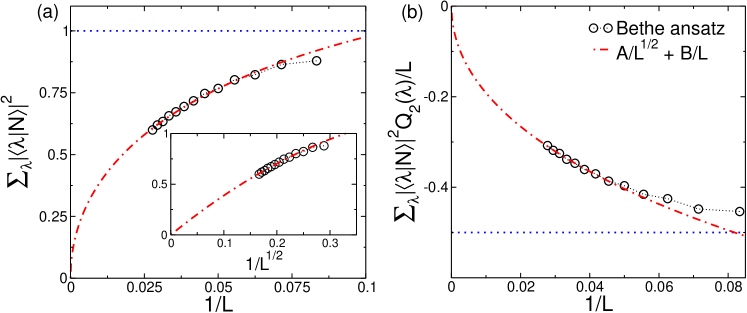
Figure 2: Overlap sum rules for the Néel state $|N\rangle$: The role of the zero-momentum strings. (a) The overlap sum rule $\sum_{\lambda}|\langle\lambda|N\rangle|^{2}=1$. Here $|\lambda\rangle$ are the eigenstates of the $XXX$ chain. The $x$-axis shows the inverse chain length $1/L$. The circles are Bethe ansatz results for chains up to $L=38$. The data are obtained by a full scanning of the Hilbert space excluding eigenstates with zero-momentum strings. The dotted line is the expected result at any $L$. The data are compatible with a vanishing behavior in the thermodynamic limit. The dash-dotted line is a fit to $A/L^{1/2}+B/L$, with $A,B$ fitting parameters. Inset: The same data as in the main Figure now plotted versus $1/L^{1/2}$. (b) The same as in (a) for the energy sum rule $\sum_{\lambda}|\langle\lambda|N\rangle|^{2}Q_{2}(\lambda)=Q_{2}^{(0)}$, with $Q_{2}(\lambda)$ the energy of the eigenstate $|\lambda\rangle$ and $Q_{2}^{(0)}/L=-1/2$ the Néel state energy density (dotted line in the Figure).

Here we study the effect of the zero-momentum strings eigenstates on the Néel overlap sum rules. We focus on the “trivial” sum rule, i.e., the normalization of the Néel state

$$\langle N|N\rangle=\sum\limits_{\lambda}|\langle\lambda|N\rangle|^{2}=1.$$ (79)

We also consider the Néel expectation value of the local conserved charge $Q_{n}$ of the $XXX$ chain (see subsection 2.5). These provide the additional sum rules

$$Q_{n}^{(0)}=\langle N|Q_{n}|N\rangle=\sum\limits_{\lambda}|\langle\lambda|N\rangle|^{2}Q_{n}(\lambda)\quad\textrm{with}\quad n\in\mathbb{N},$$ (80)

where $Q_{n}(\lambda)$ are the charges eigenvalues over the generic Bethe state $|\lambda\rangle$ (cf. (55) and (56)). In (80) $Q_{n}^{(0)}$ is the expectation value of $Q_{n}$ over the initial Néel state. $Q_{n}^{(0)}$ have been calculated in Ref. [33] for any $n$. Due to the locality of $Q_{n}$, the translational invariance of the initial state, and the periodic boundary conditions, the density $Q_{n}^{(0)}/L$ does not depend on the length of the chain.

Now we consider the sums (79) and (80) (for $n=2$, i.e., the energy sum rule) restricted to the eigenstates with no zero-momentum strings. These are shown in Figure 2 (a) and (b), respectively. Note that $Q^{(0)}_{2}/L=-1/2$ in (80) (horizontal dotted line). The circles in Figure 2 (a) are the Bethe ansatz results excluding the zero momentum strings. The data are the same as in Figure 1. The sum rules are plotted against the inverse chain length $1/L$, for $L\leq 38$. As expected, both the sum rules are strongly violated, due to the exclusion of the to zero-momentum strings. Moreover, in both Figure 2 (a) and (b) the data suggest a vanishing behavior upon increasing $L$. The dash-dotted lines are fits to $A/L^{1/2}+B/L$, with $A,B$ fitting parameters. Interestingly, the behavior as $\propto L^{-1/2}$ of the sum rules reflects that of the fraction of non-zero momentum string eigenstates $\widetilde{Z}_{Neel}/Z_{Neel}$. Specifically, from (77) and (78) it is straightforward to derive that for $L\to\infty$

$$\frac{\widetilde{Z}_{Neel}}{Z_{Neel}}\propto\frac{4}{\sqrt{\pi L}}.$$ (81)

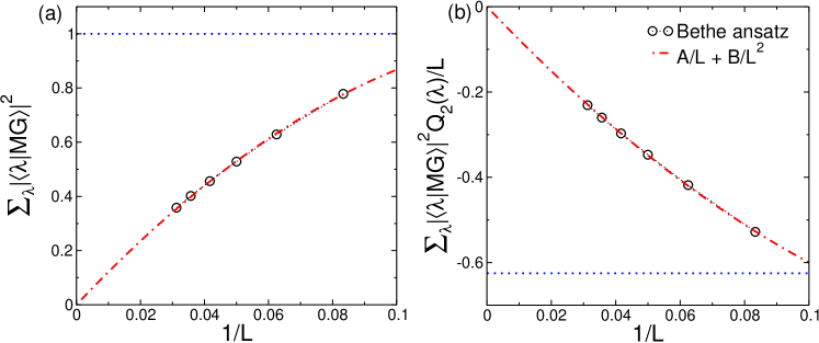
Figure 3: Overlap sum rules for the Majumdar-Ghosh state $|MG\rangle$: The role of the zero-momentum strings. (a) The sum rule $\sum_{\lambda}|\langle\lambda|MG\rangle|^{2}=1$, with $|\lambda\rangle$ the eigenstates of the $XXX$ chain. The $x$-axis plots the inverse chain length $1/L$. The circles are Bethe ansatz results for chains up to $L=32$. The results are obtained by a full scanning of the chain Hilbert space excluding eigenstates with zero-momentum strings. The dash-dotted line is a fit to $A/L+B/L^{2}$, with $A,B$ fitting parameters. (b) The same as in (a) for the energy sum rule $\sum_{\lambda}|\langle\lambda|MG\rangle|^{2}Q_{2}(\lambda)=Q_{2}^{(0)}$, with $Q_{2}(\lambda)$ the energy of $|\lambda\rangle$ and $Q_{2}^{(0)}/L=-5/8$ the Majumdar-Ghosh energy density (dotted line in the Figure).

The large $L$ behavior as $L^{-1/2}$ of the restricted sum rules is not generic, meaning that it depends on the pre-quench initial state $|\Psi_{0}\rangle$. This is illustrated in Figure 3, focusing on the Majumdar-Ghosh (MG) state. As for the Néel state, only parity-invariant eigenstates can have non-zero Majumdar-Ghosh overlap. Their total number $Z_{MG}$ (cf. (44)) is given as

$$Z_{MG}=B\Big{(}\frac{L}{2}-1,\frac{L}{4}-1\Big{)}+B\Big{(}\frac{L}{2}-1,\frac{L}{4}-1\Big{)}.$$ (82)

As for (77), $Z_{MG}$ is only un upper bound for the number of Bethe states with non-zero Majumdar-Ghosh overlaps. Note also that at any size $L$ one has $Z_{MG}<Z_{Neel}$. This is due to the Majumdar-Ghosh state being invariant under $SU(2)$ rotations, since it contains only spin singlets. In contrast with the Néel state, this implies that the Majumdar-Ghosh stat has non-zero overlap only with the $S^{z}_{T}=0$ sector of the $XXX$ chain spectrum. After restricting to the situation with no zero-momentum strings, the total number of parity-invariant eigenstates $\widetilde{Z}_{MG}$ in the sector with $S_{T}^{z}=0$ is now (cf. (50))

$$\widetilde{Z}_{MG}=B\Big{(}\frac{L}{2},\frac{L}{4}\Big{)}-B\Big{(}\frac{L}{2},\frac{L}{4}-1\Big{)}.$$ (83)

Panels (a) and (b) in Figure 3 report the restricted sums (79) and (80) for the Majumdar-Ghosh state. The data are obtained using the analytic results for the overlaps in subsection 3.3. The expected value for the energy density sum rule is $Q_{2}^{(0)}=-5/8$ (horizontal dotted line in Figure 3 (b)). Similar to Figure 2, due to the exclusion of the zero-momentum strings, the sum rules are violated, exhibiting vanishing behavior in the thermodynamic limit. However, in contrast with the Néel case, one has the behavior as $1/L$, as confirmed by the fits (dash-dotted lines in Figure 3). The vanishing of the sum rules in the thermodynamic limit reflects the behavior of $\widetilde{Z}_{MG}/Z_{MG}$ as (see (82) and (83))

$$\frac{\widetilde{Z}_{MG}}{Z_{MG}}=\frac{4}{4+L}.$$ (84)

5.3 Quench action reweighting

The results in the previous section could lead to the erroneous conclusion that the states with zero momentum strings are essential in order to reconstruct the thermodynamic values of any observables, in stark contrast with the quench action results [50, 51] that fit perfectly with the numerical simulations reported in the same papers. The solution to this apparent paradox is understood within the quench action formalism, which predicts that the representative state of the stationary state in the thermodynamic limit can be completely described restricting to the states without zero momentum strings. However, when reconstructing this state (both analytically and numerically), it must be properly normalised to unity in the reduced subspace we are considering. Consequently, we expect that after a quench from the initial state $\Psi_{0}$ the stationary expectation value of any local observables ${\cal O}$ can rewritten as

$$\langle{\cal O}\rangle=\frac{\sum_{\lambda}|\langle\lambda|\Psi_{0}\rangle|^{2}\langle\lambda|{\mathcal{O}}|\lambda\rangle}{\sum_{\lambda}|\langle\lambda|\Psi_{0}\rangle|^{2}},\qquad w_{\Psi_{0}}\equiv\sum_{\lambda}|\langle\lambda|\Psi_{0}\rangle|^{2}\,,$$ (85)

where, crucially, the sums over $\lambda$ are restricted to the states without zero momentum strings. This means that any local observable must be reweighed by the factor $w_{\Psi_{0}}$, reflecting the fact that we are considering only a small portion of the total Hilbert space.

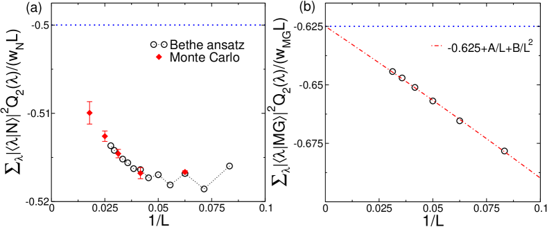
Figure 4: Energy density expectation values for a quench from Néel (a) and Majumdar-Ghosh state (b) obtained by means of the reweighting (85). For the Majumdar-Ghosh state a quadratic fit (forcing the asymptotic value $Q_{2}^{(0)}=-5/8$) describes perfectly the reweighed data. For the Néel state we also report the Monte Carlo data obtained in the next section, showing perfect agreement with the reweighed Bethe ansatz data.

The results obtained by reweighting the data in Figs. 2 and 3 are shown in Fig. 4 focusing on the conserved energy density for both the Néel and Majumdar-Ghosh initial states. It is evident that the data after reweighting approach a finite value for large $L$ in contrast with the bare vanishing values (cf. Figs. 2 and 3). It is, however, also clear that this procedure introduces some finite size corrections due to the restriction of the Hilbert space that is only justified in the thermodynamic limit. For the Majumdar-Ghosh state these corrections are monotonous and one can extrapolate with a quadratic fit in $1/L$ to infinite size, in order to reproduce the correct thermodynamic expectation (see Fig. 4 panel (b)). For the Néel initial state instead, the corrections to the scaling are not monotonous and an extrapolation based only on the data up to $L=38$ are inconclusive. In Fig. 4 we plot on top of the exact Bethe ansatz data, also Monte Carlo results obtained by sampling the restricted Hilbert space (see next section). The Monte Carlo allows to consider larger system sizes, which turns out to be enough for a good extrapolation, as we will discuss in the next section. We limit here to notice that the agreement between exact and Monte Carlo data is excellent, corroborating the correctness of both approaches.

6 Monte Carlo implementation of the quench action approach

In this section, by generalizing the results in [73], we present a Monte Carlo implementation of the quench action approach for the Néel quench in the $XXX$ chain. The key idea is to sample the eigenstates of the finite-size $XXX$ chain with the quench action probability distribution, given in (71). Similar Monte Carlo techniques to sample the Hilbert space of integrable models have been used in Ref. [78, 79, 80]. Importantly, here we consider a truncated Hilbert space, restricting ourselves to the eigenstates corresponding to solutions of the BGT equations with no zero-momentum strings. Our main physical result is that, despite this restriction, the remaining eigenstates contain enough information to correctly reproduce the post-quench thermodynamic behavior of the $XXX$ chain.

In subsection 6.1 we detail the Monte Carlo algorithm. In subsection 6.2 we numerically demonstrate that after the Monte Carlo “resampling” the Néel sum rules (80) are restored, in the thermodynamic limit. The Hilbert space truncation is reflected only in $\propto 1/L$ finite-size corrections to the sum rules. In the Bethe ansatz language the eigenstates sampled by the Monte Carlo become equivalent to the quench action representative state in the thermodynamic limit. Here this is explicitly demonstrated by numerically extracting the quench action root distributions $\boldsymbol{\rho}^{*}$ (cf. (74)-(76)). The numerical results are found in remarkable agreement with the quench action.

6.1 The quench action Monte Carlo algorithm

The Monte Carlo procedure starts with a randomly selected parity-invariant eigenstate (Bethe state) of the $XXX$ chain, in the sector with zero magnetization, i.e., $M=L/2$ particles. As the Néel state is not invariant under $SU(2)$ rotations, in order to characterize the Bethe states one has to specify the number $N_{\infty}$ of infinite rapidities (see 2.1). The number of remaining particles corresponding to finite BGT rapidities $M^{\prime}$ is $M^{\prime}=L/2-N_{\infty}$. The Bethe state is identified by a parity-invariant BGT quantum number configuration that we denote as ${\mathcal{C}}$. Due to the parity-invariance and the zero-momentum strings being excluded, ${\mathcal{C}}$ is identified by the number $m^{\prime}$ of parity-invariant quantum numbers $\{\pm I_{j}\}_{j=1}^{m^{\prime}}$ (equivalently, root pairs $\{\pm\lambda_{j}\}_{j=1}^{m^{\prime}}$). The string content associated with the state is denoted as $\widetilde{\mathcal{S}}=\{\tilde{s}_{1},\dots,\tilde{s}_{m^{\prime}}\}$, where $\tilde{s}_{n}$ is the number of pairs of $n$-strings. The Monte Carlo procedure generates a new parity-invariant eigenstate of the $XXX$ chain, and it consists of four steps:

1. Choose a new number of finite-momentum particles $M^{\prime\prime}$ and of parity-invariant rapidity pairs $m^{\prime\prime}\equiv M^{\prime\prime}/2$ with probability ${\mathcal{P}}(M^{\prime\prime})$ as

   $${\mathcal{P}}(M^{\prime\prime})=\frac{\widetilde{Z}^{\prime}_{Neel}(L,M^{\prime\prime})}{\widetilde{Z}_{Neel}(L)},$$ (86)

   where $\widetilde{Z}_{Neel}(L)$ is defined in (78), and $\widetilde{Z}^{\prime}_{Neel}$ is the number of parity-invariant eigenstates with no zero-momentum strings in the sector with fixed particle number $M^{\prime\prime}$ (cf. (49) for the precise expression).

2. Choose a new string content $\widetilde{\mathcal{S}}^{\prime}\equiv\{\tilde{s}_{1}^{\prime},\dots,\tilde{s}^{\prime}_{m^{\prime\prime}}\}$ with probability ${\mathcal{P}}^{\prime}(M^{\prime\prime},\widetilde{\mathcal{S}}^{\prime})$

   $${\mathcal{P}}^{\prime}(M^{\prime\prime},\widetilde{\mathcal{S}}^{\prime})=\frac{1}{\widetilde{Z}^{\prime}_{Neel}(L,M^{\prime\prime})}\prod_{n=1}^{m^{\prime\prime}}B\Big{(}\frac{L}{2}-\sum\limits_{l=1}^{m^{\prime\prime}}t_{nl}\tilde{s}^{\prime}_{l},\tilde{s}^{\prime}_{n}\Big{)},$$ (87)

   where the matrix $t_{nl}$ is defined in (18).

3. Generate a new parity-invariant quantum number configuration ${\mathcal{C}}^{\prime}$ compatible with the $\widetilde{\mathcal{S}}^{\prime}$ obtained in step . Solve the corresponding BGT equations (14), finding the rapidities $\{\pm\lambda^{\prime}_{j}\}_{j=1}^{m^{\prime\prime}}$ of the new parity-invariant eigenstate.

4. Calculate the Néel overlap $\langle\{\pm\lambda^{\prime}_{j}\}_{j=1}^{m^{\prime\prime}}|N\rangle$ for the new eigenstate, using (58) (61) (62) and (63). Accept the new eigenstate with the quench action Metropolis probability

   $${\mathcal{P}}^{\prime\prime}_{\lambda\to\lambda^{\prime}}=\textrm{Min}\Big{\{}1,\exp\Big{(}-2{\rm Re}({\mathcal{E}}^{\prime}-{\mathcal{E}})\Big{)}\Big{\}},$$ (88)

   where ${\mathcal{E}}^{\prime}\equiv-\ln\langle\{\pm\lambda^{\prime}_{j}\}_{j=1}^{m^{\prime\prime}}|N\rangle$, ${\mathcal{E}}\equiv-\ln\langle\{\pm\lambda_{j}\}_{j=1}^{m^{\prime\prime}}|N\rangle$.

Note that while the steps $1$-$3$ account for the string content and particle number probabilities of the parity-invariant states, step $4$ assigns to the different eigenstates the correct quench action probability.

For a generic local observable ${\mathcal{O}}$, its quench action expectation $\langle{\mathcal{O}}\rangle$ is obtained as the arithmetic average of the eigenstates expectation values $\langle\lambda|{\mathcal{O}}|\lambda\rangle$, with $|\lambda\rangle$ the eigenstates sampled by the Monte Carlo, as

$$\langle{\mathcal{O}}\rangle=\frac{1}{N_{mcs}}\sum\limits_{\lambda}\langle\lambda|{\mathcal{O}}|\lambda\rangle.$$ (89)

Here $N_{mcs}$ is the total number of Monte Carlo steps. Note that, as usual in Monte Carlo, some initial steps have to be neglected to ensure equilibration. Note that (89) can be used for any observable ${\mathcal{O}}$ for which the the Bethe state expectation value $\langle\lambda|{\mathcal{O}}|\lambda\rangle$ (form factor) is known.

Finally, it is worth stressing that although the Monte Carlo sampling is done only on the zero-momentum free Hilbert subspace, the algorithm does not suffer of the reweighting problems found in the exact method (see the preceding section), because the expectation values (89) are automatically normalised by the factor $N_{mcs}$.

6.2 The Néel overlap sum rules: Monte Carlo results

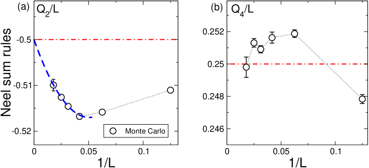
Figure 5: The overlap sum rules for the Néel state $|N\rangle$ in the Heisenberg spin chain: Numerical results obtained by the Monte Carlo sampling of the chain Hilbert space. In all panels the $x$ axis shows the inverse chain length $1/L$ (a) The energy sum rule $\sum_{\lambda}|\langle N|\lambda\rangle|^{2}Q_{2}(\lambda)/L=Q^{(0)}_{2}$, with $|\lambda\rangle$ the generic eigenstate of the $XXX$ chain, $Q_{2}(\lambda)/L$ the associated energy density, and $Q_{2}^{(0)}=-1/2$ the Néel energy density. The symbols are Monte Carlo data. The dash-dotted line is the expected result $Q_{2}^{(0)}$. The dashed line is a fit to the behavior $-1/2+A/L+B/L^{2}$, with $A,B$ fitting parameters. (b) Same as in (a) for the charge $Q_{4}$ without the fit.

The validity of the Monte Carlo approach outlined in 6.2 is demonstrated in Fig. 5. The Figure focuses on the Néel overlap sum rules for the conserved charges densities $Q_{2}/L$ and $Q_{4}/L$ (cf. subsection 2.5 for the definition of the charges, and (80) for the associated sum rules). Note that in (80) the sum is now over the eigenstates $|\lambda\rangle$ sampled by the Monte Carlo. Panel (a) in Figure 5 reports the sum rule for the energy density $Q_{2}/L$ (these are the same data reported in Fig. 4 which perfectly agree with the exact data, corroborating the accuracy of the Monte Carlo sampling). The circles in the Figure are Monte Carlo data for the Heisenberg chain with $L\leq 56$ sites. The data correspond to Monte Carlo simulations with $N_{mcs}\sim 10^{7}$ Monte Carlo steps (mcs). In all panels the $x$-axis shows the inverse chain length $1/L$.

Clearly, the Monte Carlo data suggest that in the thermodynamic limit the Néel overlap sum rules (80) are restored, while violations are present for finite chains. This numerically confirms that the truncation of the Hilbert space, i.e., removing the zero-momentum strings, gives rise only to scaling corrections, while the thermodynamic behavior after the quench is correctly reproduced. Note that the data in panel (a) are suggestive of the behavior $\propto 1/L$ for the scaling corrections, as confirmed by the fit to $-1/2+A/L+b/L^{2}$ (dashed line in the Figure), with $A,B$ fitting parameters.

Similarly, panel (b) in Figure 5 reports the charge density $Q_{4}/L$. Also in this case, the Monte Carlo data for $L=48$ are already compatible with the expected result $Q_{4}/L=1/4$ in the thermodynamic limit. The scaling corrections are however not monotonous and it is impossible to proceed to a proper extrapolation to the thermodynamic limit. This could be attributed to fact that the support of $Q_{n}$, i.e., the number of sites where the operator acts non trivially, increases linearly with $n$ (see [75] for the precise expression). Anyhow, notice that all data deviate from the expected asymptotic value for about 1%.

6.3 Extracting the quench action root distributions

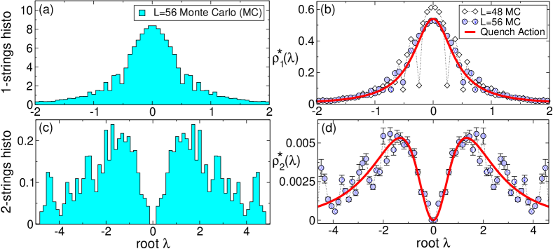
Figure 6: The quench action root distributions $\rho^{*}_{1}(\lambda)$ and $\rho^{*}_{2}(\lambda)$ for the $1$-strings and $2$-strings, respectively: Monte Carlos results. (a) The histograms of the $1$-string Bethe-Gaudin-Takahashi (BGT) roots $\lambda$ sampled in the Monte Carlo. The data are for a chain with $L=56$ sites and a Monte Carlo history with $N_{mcs}\sim 10^{7}$ Monte Carlo steps. The $y$-axis is divided by a factor $10^{6}$ for convenience. (c) The same as in (a) for the $2$-string roots. (b) The $1$-string root distribution $\rho^{*}_{1}(\lambda)$ plotted versus $\lambda$ for two chains with $L=48$ and $L=56$ (diamond and circles, respectively). The full line is the quench action analytic result in the thermodynamic limit. (d) The same as in (b) for the $2$-string root distribution $\rho^{*}_{2}(\lambda)$. In both (b) and (d) the oscillations are finite-size effects, whereas the error bars are the statistical Monte Carlo errors.

The BGT root distributions corresponding to the quench action steady state (cf. (74)-(76)) $\boldsymbol{\rho^{*}}=\{\rho^{*}_{n}(\lambda)\}_{n=1}^{\infty}$ can be extracted from the Monte Carlo simulation, similar to what has been done in Ref. [73] for the Generalized Gibbs Ensemble (GGE) representative state. The idea is that for the local observables considered here, in each eigenstate expectation value $\langle\lambda|{\mathcal{O}}|\lambda\rangle$ in (89) one can isolate the contribution of the different string sectors as

$$\langle\lambda|{\mathcal{O}}|\lambda\rangle=\sum\limits_{n,\gamma}{\mathcal{O}}_{n}(\lambda_{n;\gamma}).$$ (90)

Here ${\mathcal{O}}_{n}$ is the contribution of the BGT $n$-strings to the expectation value of ${\mathcal{O}}$, and $\pm\lambda_{n;\gamma}$, with $\gamma$ labeling the different $n$-strings, are the solutions of the BGT equations (14) identifying the Bethe state $|\lambda\rangle$. We should stress again that (90) is true only for local or quasi-local observables, while generic observables are more complicated functions of the rapidities. By comparing (89) and (73) one obtains that in the limit $L,N_{mcs}\to\infty$

$$\quad\lim_{N_{mcs}\to\infty}\,\frac{1}{N_{mcs}}\sum\limits_{\lambda_{n;\gamma}}{\mathcal{O}}_{n}(\lambda_{n;\gamma})\,\stackrel{{\scriptstyle L\to\infty}}{{\overrightarrow{\hskip 40.0pt}}}\,\langle\boldsymbol{\rho^{*}}|{\mathcal{O}}|\boldsymbol{\rho^{*}}\rangle\equiv\sum_{n}\int_{-\infty}^{+\infty}d\lambda\rho^{*}_{n}(\lambda){\mathcal{O}}_{n}(\lambda).$$ (91)

This suggests that the histogram of the $n$-strings BGT roots sampled in the Monte Carlo converges in the thermodynamic limit to the saddle point root distribution $\rho^{*}_{n}(\lambda)$.

This is demonstrated numerically in Figure 6 considering $\rho^{*}_{1}(\lambda)$ (panels (a)(b)) and $\rho^{*}_{2}(\lambda)$ (panel (c)(d)). The histograms correspond to Monte Carlo data for $L=48$ and $L=56$ sites. Panel (a) and (c) show the histograms of the $1$-string and $2$-string BGT roots sampled in the Monte Carlo. The $y$-axis is rescaled by a factor $10^{6}$ for convenience. The width of the histogram bins $\Delta\lambda$ is $\Delta\lambda\approx 0.02$ and $\Delta\lambda\approx 0.001$ for $\rho_{1}(\lambda)$ and $\rho_{2}(\lambda)$, respectively. The histogram fluctuations are due both to the finite statistics (finite $N_{mcs}$) and to the finite size of the chain.

The extracted quench-action root distributions $\rho^{*}_{1}(\lambda)$ and $\rho^{*}(\lambda)$ are shown in panels (b) and (d). The data are the same as in panel (a)(c). The normalization of the distributions is chosen such as to match the analytical results from (74) and (75), i.e., $\int d\lambda\rho^{*}_{1}(\lambda)\approx 0.31$ and $\int d\lambda\rho^{*}_{2}(\lambda)\approx 0.015$. The Monte Carlo error bars shown in the Figure are obtained with a standard jackknife analysis [81, 82]. The continuous lines are the expected analytic results in the thermodynamic limit (cf. (74) (75)).

Clearly, the Monte Carlo data are in excellent agreement with (74) in the whole range $-2\leq\lambda\leq 2$ considered. For $\rho^{*}_{1}(\lambda)$ the statistical error bars are smaller than the symbol size. The oscillating corrections around $|\lambda|\sim 0.5$ are lattice effects, which decrease with increasing the chain size (see the data for $L=48$ in the Figure). Much larger finite-size effects are observed for $\rho^{*}_{2}(\lambda)$ (panel (d) in the Figure). Specifically, the corrections are larger on the tails of the root distribution. Moreover, the Monte Carlo error bars are clearly larger than for $\rho_{1}^{*}(\lambda)$. This is due to the fact that since $\int d\lambda\rho^{*}_{2}(\lambda)/\sum_{n}\int d\lambda\rho_{n}^{*}(\lambda)\approx 0.04$, the Monte Carlo statistics available for estimating $\rho_{2}^{*}(\lambda)$ is effectively reduced as compared to $\rho_{1}^{*}(\lambda)$. Finally, we numerically observed that finite-size corrections and Monte Carlo error bars are even larger for the $3$-strings root distribution $\rho^{*}_{3}(\lambda)$, which makes its numerical determination more difficult.

7 Conclusions

We developed a finite size implementation of the quench action method for integrable models. We focused on the spin-$1/2$ isotropic Heisenberg ($XXX$) chain, considering simple product states as initial states, but the approach is of general validity. The main ingredient of the approach is the knowledge of the overlaps between the pre-quench states and the $XXX$ chain eigenstates (that for the cases at hand have been obtained recently [69, 66, 67, 68, 70]). For chains up to about 40 spins the (relevant part of the) Hilbert space can be fully spanned, while for large systems we performed an effective Monte Carlo sampling. The main outcome of the method is a precise determination of the root distributions which allow then the determination of local observables by standard methods. Thermodynamic quantities are finally extracted using finite-size scaling. The main result of this papers have been already summarised in the introductory section and we limit here to some discussions about further developments.

First of all, the importance of the proposed method relies on the property that the only required ingredient is the (analytical or even numerical) knowledge of the overlaps between the initial state and the Bethe states. For this reason, it can be implemented even in cases in which an analytic thermodynamic solution is not available.

Another interesting consequence of our work is that we can use a vanishing fraction of the eigenstates in order to determine the thermodynamic behavior. It is clearly interesting to understand whether there are other clever ways to further reduce the fraction of considered states (without knowing the exact solution, when we can just pinpoint one representative eigenstate).

Finally, it is an open interesting issue to understand how the present method can be used to describe the time evolution of a finite but large system and in particular how to reconstruct the time evolution from a vanishing fraction of relevant eigenstates, eventually mimicking the strategy employed in thermodynamic limit [54, 55].

Appendix A Exact Néel and Majumdar-Ghosh overlaps for a small Heisenberg chain

In this section we provide exact diagonalization results for the overlaps between the Néel state and the Majumdar-Ghosh (MG) state and all the eigenstates of the Heisenberg spin chain with $L=12$ sites. For the eigenstates without zero-momentum strings, we also provide the overlaps obtained using the string hypothesis (58)(64). This allows to check the validity of the string hypothesis when calculating overlaps. Moreover, this also provides a simple check of the counting formula (28).

A.1 Néel overlap

Bethe states with nonzero Néel overlap ($L=12$)
String content $2I_{n}$ $q$ E $|\langle\lambda|N\rangle|^{2}$ (exact) $|\langle\lambda|N\rangle|^{2}$ (BGT) 6 inf - - $0$ $0.002164502165$ $0.002164502165$ {2,0}  4 inf $1_{1}$ $2$ $-3.918985947229$ $0.096183409244$ $0.096183409244$ $3_{1}$ $-3.309721467891$ $0.011288497947$ $0.011288497947$ $5_{1}$ $-2.284629676547$ $0.004542580506$ $0.004542580506$ $7_{1}$ $-1.169169973996$ $0.002752622983$ $0.002752622983$ $9_{1}$ $-0.317492934338$ $0.002116006203$ $0.002116006203$ {4,0,0,0}  2 inf $1_{1}3_{1}$ $4$ $-7.070529325964$ $0.310133033838$ $0.310133033838$ $1_{1}5_{1}$ $-5.847128730477$ $0.129277023687$ $0.129277023687$ $1_{1}7_{1}$ $-4.570746557876$ $0.085992436024$ $0.085992436024$ $3_{1}5_{1}$ $-5.153853093221$ $0.015256395523$ $0.015256395523$ $3_{1}7_{1}$ $-3.916336243695$ $0.010091113504$ $0.010091113504$ $5_{1}7_{1}$ $-2.817696043731$ $0.004059780228$ $0.004059780228$ {0,2,0,0}  2 inf $1_{2}$ $2$ $-1.905667167442$ $0.001207238321$ $0.0012072{\color[rgb]{1,0,0}45406}$ $3_{2}$ $-1.368837200825$ $0.002340453815$ $0.0023{\color[rgb]{1,0,0}25724713}$ $5_{2}$ $-0.681173793635$ $0.001921010489$ $0.0019{\color[rgb]{1,0,0}39001396}$ {1,0,1,0}  2 inf $0_{1}0_{3}$ $2$ $-2.668031843135$ $0.034959609810$ - {6,0,0,0,0,0}  0 inf $1_{1}3_{1}5_{1}$ $6$ $-8.387390917445$ $0.153412152966$ $0.153412152966$ {2,2,0,0,0,0}  0 inf $1_{1}1_{2}$ $4$ $-5.401838225870$ $0.040162686361$ $0.04{\color[rgb]{1,0,0}1042488913}$ $3_{1}1_{2}$ $-4.613929948329$ $0.004636541934$ $0.004{\color[rgb]{1,0,0}730512604}$ $5_{1}1_{2}$ $-3.147465758841$ $0.001335522556$ $0.00133{\color[rgb]{1,0,0}7334035}$ {3,0,1,0,0,0}  0 inf $0_{1}2_{1}0_{3}$ $4$ $-6.340207488736$ $0.052743525774$ - $0_{1}4_{1}0_{3}$ $-5.203653009936$ $0.015022005621$ - $0_{1}6_{1}0_{3}$ $-3.788693957250$ $0.011144489334$ - {1,0,0,0,1,0}  0 inf $0_{1}0_{5}$ $2$ $-2.444293750583$ $0.005887902992$ - {0,0,2,0,0,0}  0 inf $1_{3}$ $2$ $-1.111855930538$ $0.001342476001$ $0.0013{\color[rgb]{1,0,0}84980817}$ {0,1,0,1,0,0}  0 inf $0_{2}0_{4}$ $2$ $-1.560671012472$ $0.000026982174$ -

Table 1: All Bethe states for $L=12$ having nonzero overlap with the Néel state. The first column shows the string content of the Bethe states, including the number of infinite rapidities. The second and third column show $2I_{n}$, with $I_{n}$ the BGT quantum numbers identifying the different states, and the number $q$ of independent strings. Due to the parity invariance, only positive quantum numbers are reported. In the second column only the positive BGT numbers are shown. The fourth column is the Bethe state eigenenergy. Finally, the last two columns show the exact overlap with the Néel state and the approximate result obtained using the BGT equations. In the last column Bethe states containing zero-momentum strings are excluded. Deviations from the exact result (digits with different colors) are attributed to the string hypothesis.

The overlaps between all the eigenstates of the Heisenberg spin chain and the Néel state are reported in Table 1. The first column in the Table shows the string content ${\mathcal{S}}\equiv\{s_{1},\dots,s_{M}\}$, with $M$ being the number of finite rapidities. The number of infinite rapidities $N_{\infty}=L/2-M$ (see section 2.1) is also reported. The second column shows $2I_{n}$, with $I_{n}$ the Bethe-Gaudin-Takahashi quantum numbers (see section 2.2) identifying the $XXX$ chain eigenstates. Due to the parity invariance, only the positive quantum numbers are reported. The total number of independent strings, i.e., $q\equiv\sum_{j}s_{j}$, is shown in the third column. The fourth column is the eigenstates energy eigenvalue $E$. The last two columns show the squared Néel overlaps and the corresponding result obtained using the Bethe-Gaudin-Takahashi equations, respectively. In the last column only the case with no zero-momentum strings is considered. The deviations from the exact diagonalization results (digits with different colors) have to be attributed to the string hypothesis. Notice that the overlap between the Néel state and the $S_{z}=0$ eigenstate in the sector with maximal total spin $S=L/2$ (first column in Table 1), is given analytically as $2/B(L,L/2)$, with $B(x,y)$ the Newton binomial.

Some results for a larger chain with $L=20$ sites are reported in Figure 7. The squared overlaps $|\langle\lambda|N\rangle|^{2}$ between the Néel state and the $XXX$ chain eigenstates $|\lambda\rangle$ are plotted against the eigenstate energy density $E/L\in[-\ln(2),0]$. The circles are exact diagonalization results for all the chain eigenstates ($382$ eigenstates), whereas the crosses denote the overlaps calculated using formula (58). Note that only the eigenstates with no zero-momentum strings are shown ($252$ eigenstates) in the Figure. Panel (a) gives an overview of all the overlaps. Panels (b)-(d) correspond to zooming to the smaller overlap values $|\langle N|\lambda\rangle|\lesssim 0.02$, $|\langle N|\lambda\rangle|\lesssim 0.002$, and $|\langle N|\lambda\rangle|\lesssim 10^{-5}$. Although some deviations are present, the overall agreement between the exact diagonalization results and the Bethe ansatz is satisfactory, confirming the validity of the string hypothesis for overlap calculations.

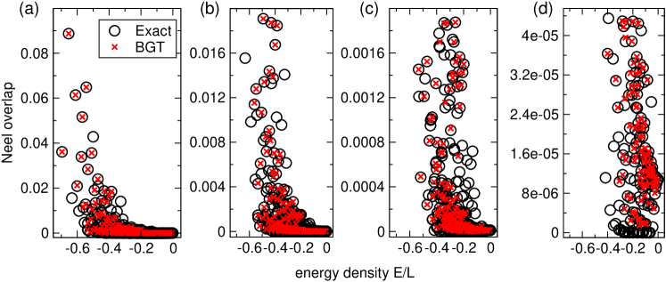
Figure 7: The squared overlap $|\langle N|\lambda\rangle|^{2}$ between the the Néel state $|N\rangle$ and the eigenstates $|\lambda\rangle$ of the $XXX$ chain with $L=20$ sites. Only non-zero overlaps are shown. In all the panels the $x$-axis shows the eigenstate energy density $E/L$. The circles are the exact diagonalization results for all the non-zero overlaps. The crosses are the Bethe ansatz results obtained using the Bethe-Gaudin-Takahashi equations. The missing crosses correspond to eigenstates containing zero-momentum strings. (a) Overview of all the non-zero overlaps. (b)(c)(d) The same overlaps as in (a) zooming in the regions $[0,0.2]$, $[0,0.020]$, and $[0,4\cdot 10^{-5}]$. The tiny differences between the ED and the Bethe ansatz results are attributed to the string deviations.

Bethe states with nonzero Néel overlap ($L=12$)
String content $2I_{n}$ $q$ E $|\langle\lambda|MG\rangle|^{2}$ (exact) $|\langle\lambda|MG\rangle|^{2}$ (BGT) {6,0,0,0,0,0} $1_{1}3_{1}5_{1}$ $6$ $-8.387390917445$ $0.716615769224$ $0.716615769224$ {2,2,0,0,0,0} $1_{1}1_{2}$ $4$ $-5.401838225870$ $0.055624700196$ $0.05{\color[rgb]{1,0,0}4033366543}$ $3_{1}1_{2}$ $-4.613929948329$ $0.005687428810$ $0.005{\color[rgb]{1,0,0}582983043}$ $5_{1}1_{2}$ $-3.147465758841$ $0.002107475934$ $0.002107{\color[rgb]{1,0,0}086933}$ {3,0,1,0,0,0} $0_{1}2_{1}0_{3}$ $4$ $-6.340207488736$ $0.205891158647$ - $0_{1}4_{1}0_{3}$ $-5.203653009936$ $0.038832154450$ - $0_{1}6_{1}0_{3}$ $-3.788693957250$ $0.006019410923$ - {1,0,0,0,1,0} $0_{1}0_{5}$ $2$ $-2.444293750583$ $0.000129601311$ - {0,0,2,0,0,0} $1_{3}$ $2$ $-1.111855930538$ $0.000011727787$ $0.00001{\color[rgb]{1,0,0}2785580}$ {0,1,0,1,0,0} $0_{2}0_{4}$ $2$ $-1.560671012472$ $0.000330572718$ -

Table 2: All Bethe states for $L=12$ having nonzero overlap with the Majumdar-Ghosh (MG) state. The first column shows the string content of the Bethe states. The second and third column show $2I_{n}$, with $I_{n}$ the BGT quantum numbers identifying the different states, and the number $q$ of independent strings. Due to the parity invariance, we show only the positive quantum numbers. In the second column only the positive BGT numbers are shown. Note that, in contrast to Table 1 no states with infinite rapidities are present. The fourth column is the Bethe state eigenenergy. Finally, the last two columns show the exact overlap with the MG state and the approximate result obtained using the BGT equations. In the last column Bethe states containing zero-momentum strings are excluded. Deviations from the exact result (digits with different colors) are attributed to the string hypothesis.

A.2 Majumdar-Ghosh overlap

The overlap between all the Heisenberg chain eigenstates with the Majumdar-Ghosh state are shown in Table 2 for the chain with $L=12$ sites. The conventions on the representation of the eigenstates is the same as in Table 1. Note that in contrast with the Néel state, only the eigenstates with zero total spin $S=0$ have non zero overlap, i.e., no eigenstates with infinite rapidities are present, which reflect that the Majumdar-Ghosh state is invariant under $SU(2)$ rotations.

References

References

- [1] I. Bloch, J. Dalibard, and W. Zwerger, Rev. Mod. Phys. 80, 885 (2008).
- [2] M. Greiner, O. Mandel, T. Hänsch, and I. Bloch, Nature (London) 419, 51 (2002).
- [3] T. Kinoshita, T. Wenger, and D. S. Weiss, Nature (London) 440, 900 (2008).
- [4] S. Hofferberth, I. Lesanovsky, B. Fischer, T. Schumm, and J. Schiedmayer, Nature (London) 449, 324 (2007).
- [5] S. Trotzky, Y.-A. Chen, A. Flesch, I. P. McCulloch, U. Schollwöck, J. Eisert, and I. Bloch, Nature Phys. 8, 325 (2012).
- [6] M. Gring, M. Kuhnert, T. Langen, T. Kitagawa, B. Rauer, M. Schreitl, I. Mazets, D. A. Smith, E. Demler, and J. Schmiedmayer, Science 337, 6100 (2012).
- [7] M. Cheneau, P. Barmettler, D. Poletti, M. Endres, P. Schaua, T. Fukuhara, C. Gross, I. Bloch, C. Kollath, and S. Kuhr, Nature (London) 481, 484 (2012).
- [8] U. Schneider, L. Hackeruller, J. P. Ronzheimer, S. Will, S. Braun, T. Best, I. Bloch, E. Demler, S. Mandt, D. Rasch, and A. Rosch, Nature Phys. 8, 213 (2012).
- [9] M. Kuhnert, R. Geiger, T. Langen, M. Gring, B. Rauer, T. Kitagawa, E. Demler, D. Adu Smith, and J. Schmiedmayer, Phys. Rev. Lett. 110, 090405 (2013).
- [10] T. Langen, R. Geiger, M. Kuhnert, B. Rauer, and J. Schmiedmayer, Nature Phys. 9, 640 (2013).
- [11] F. Meinert, M. J. Mark, E. Kirilov, K. Lauber, P. Weinmann, A. J. Daley, and H.-C. Nagerl, Phys. Rev. Lett. 111, 053003 (2013).
- [12] T. Fukuhara, A. Kantian, M. Endres, M. Cheneau, P. Schaua, S. Hild, C. Gross, U. Schollwöck, T. Giamarchi, I. Bloch, and S. Kuhr, Nature Phys. 9, 235 (2013).
- [13] J. P. Ronzheimer, M. Schreiber, S. Braun, S. S. Hodgman, S. Langer, I. P. McCulloch, F. Heidrich-Meisner, I. Bloch, and U. Schneider, Phys. Rev. Lett. 110, 205301 (2013).
- [14] S. Braun, M. Friesdorf, S. Hodgman, M. Schreiber, J. Ronzheimer, A. Riera, M. del Rey, I. Bloch, J. Eisert, and U. Schneider, PNAS 112, 3641 (2015).
- [15] T. Langen, S. Erne, R. Geiger, B. Rauer, T. Schweigier, M. Kuhnert, W. Rohringer, I. E. Mazets, T. Gasenzer, J. Schmiedmayer, Science 348, 6231 (2015).
- [16] A. Polkovnikov, K. Sengupta, A Silva, and M. Vengalattore, Rev. Mod. Phys. 83, 863 (2011).
-
[17]
J. Eisert, M. Friesdorf, and C. Gogolin, Nature Phys. 11, 124 (2015);
C. Gogolin and J. Eisert, arXiv:1503.07538. - [18] J. M. Deutsch, Phys. Rev. A 43, 2046 (1991).
- [19] M. Srednicki, Phys. Rev. E 50, 888 (1994).
-
[20]
G. Biroli, C. Kollath, and A. Laeuchli, Phys. Rev. Lett. 105, 250401 (2010);
M. C. Banuls, J. I. Cirac, and M. B. Hastings, Phys. Rev. Lett. 106, 050405 (2011);
M. Rigol and M. Fitzpatrick, Phys. Rev. A 84, 033640 (2011);
K. He and M. Rigol, Phys. Rev. A 85, 063609 (2012);
G. P. Brandino, A. De Luca, R. M. Konik, and G. Mussardo, Phys. Rev. B 85, 214435 (2012);
M. Rigol and M. Srednicki, Phys. Rev. Lett. 108, 110601 (2012);
J. Sirker, N.P. Konstantinidis, and N. Sedlmayr, Phys. Rev. A 89, 042104 (2014);
T. M. Wright, M. Rigol, M. J. Davis, and K. V. Kheruntsyan, Phys. Rev. Lett. 113, 050601 (2014);
M. Rigol, ArXiv:1511.04447. -
[21]
T. N. Ikeda, Y. Watanabe, and M. Ueda, Phys. Rev. E 87, 012125 (2013);
V. Alba, Phys. Rev. B 91, 155123 (2015). - [22] M. Rigol, V. Dunjko, V. Yurovsky, and M. Olshanii, Phys. Rev. Lett. 98, 050405 (2007).
- [23] M. Rigol, V. Dunjko, and M. Olshanii, Nature 452, 854 (2008).
-
[24]
P. Calabrese and J. Cardy, Phys. Rev. Lett. 96, 136801 (2006);
P. Calabrese and J. Cardy, J. Stat. Mech. (2007) P06008. -
[25]
M. Cramer, C. M. Dawson, J. Eisert, and T. J. Osborne, Phys. Rev. Lett. 100, 030602 (2008);
M. Cramer and J. Eisert, New J. Phys. 12, 055020 (2010). - [26] T. Barthel and U. Schollwöck, Phys. Rev. Lett. 100, 100601 (2008).
-
[27]
D. Rossini, A. Silva, G. Mussardo, and G. E. Santoro, Phys. Rev. Lett. 102, 127204 (2009);
D. Rossini, S. Suzuki, G. Mussardo, G. E. Santoro, and A. Silva, Phys. Rev. B 82, 144302 (2010). -
[28]
P. Calabrese, F. H. L. Essler, and M. Fagotti, Phys. Rev. Lett. 106, 227203 (2011);
P. Calabrese, F. H. L. Essler, and M. Fagotti, J. Stat. Mech. (2012) P07016;
P. Calabrese, F. H. L. Essler, and M. Fagotti, J. Stat. Mech. (2012) P07022;
F. H. L. Essler, S. Evangelisti, and M. Fagotti, Phys. Rev. Lett. 109, 247206 (2012). -
[29]
M. A. Cazalilla, Phys. Rev. Lett. 97, 156403 (2006);
A. Iucci and M. A. Cazalilla, Phys. Rev. A 80, 063619 (2009);
A. Iucci and M. A. Cazalilla New J. Phys. 12, 055019 (2010);
M. A. Cazalilla, A. Iucci, and M.-C. Chung, Phys. Rev. E 85, 011133 (2012). - [30] D. Schuricht and F. H. L. Essler, J. Stat. Mech. P04017 (2012).
- [31] J. Mossel and J.-S. Caux, New J. Phys. 14 075006 (2012).
-
[32]
M. Collura, S. Sotiriadis and P. Calabrese, Phys. Rev. Lett. 110, 245301 (2013);
M. Collura, S. Sotiriadis and P. Calabrese, J. Stat. Mech. P09025 (2013). - [33] M. Fagotti and F. H. L. Essler, Phys. Rev. B 87, 245107 (2013).
- [34] M. Kormos, M. Collura, and P. Calabrese, Phys. Rev. A 89, 013609 (2014).
- [35] P. P. Mazza, M. Collura, M. Kormos, and P. Calabrese, J. Stat. Mech. (2014) P11016.
- [36] S. Sotiriadis and P. Calabrese, J. Stat. Mech. (2014) P07024.
-
[37]
M. Fagotti, Rev. B 87, 165106 (2013);
L. Bucciantini, M. Kormos, and P. Calabrese, J. Phys. A 47, 175002 (2014). - [38] E. Ilieveski, J. De Nardis, B. Wouters, J.-S. Caux, F. H. Essler, and T. Prosen, Phys. Rev. Lett. 115, 157201 (2015).
- [39] J. Cardy, arXiv:1507.07266.
- [40] T. Prosen, Nucl. Phys. B 886, (2014) 1177.
- [41] R. G. Pereira, V. Pasquier, J. Sirker, and I. Affleck, J. Stat. Mech. (2014) P09037.
- [42] E. Ilievski, M. Medejak, and T. Prosen, Phys. Rev. Lett. 115, 120601 (2015).
- [43] F. H. L. Essler, G. Mussardo, and M. Panfil, Phys. Rev. A 91, 051602 (2015).
- [44] J.-S. Caux and F. H. L. Essler, Phys. Rev. Lett. 110, 257203 (2013).
- [45] M. Takahashi, Thermodynamics of one-dimensional solvable models, Cambridge University Press, Cambridge, 1999.
- [46] J. De Nardis, B. Wouters, M. Brockmann, and J.-S. Caux, Phys. Rev. A 89, 033601 (2014).
- [47] G. Goldstein and N. Andrei, Phys. Rev. B 92, 155103 (2015).
- [48] L. Piroli, P. Calabrese, and F. H.L. Essler, arXiv:1509.08234.
- [49] L. Bucciantini, arXiv:1510.08125.
-
[50]
B. Pozsgay, M. Mestyán, M. A. Werner, M. Kormos, G. Zaránd, and G. Takács,
Phys. Rev. Lett. 113, 117203 (2014);
M Mestyán, B. Pozsgay, G. Takács, and M. A. Werner, J. Stat. Mech. (2015) P04001. -
[51]
B. Wouters, M. Brockmann, J. De Nardis, D. Fioretto, M. Rigol, and J.-S. Caux,
Phys. Rev. Lett. 113, 117202 (2014);
M. Brockmann, B. Wouters, D. Fioretto, J. De Nardis, R. Vlijm, and J.-S. Caux, J. Stat. Mech. (2014) P12009. - [52] A. De Luca, G. Martelloni, and J. Viti, Phys. Rev. A 91, 021603 (2015).
- [53] B. Bertini, D. Schuricht, and F. H. L. Essler, J. Stat. Mech. P10035 (2014).
- [54] J. De Nardis and J.-S. Caux, J. Stat. Mech. (2014) P12012.
- [55] J. De Nardis, L. Piroli, and J.-S. Caux, J. Phys. A 48, 43FT01 (2015).
- [56] H. Bethe, Z. Phys. 71, 205 (1931).
- [57] V. E. Korepin, N. M. Bogoliubov, and A. G. Izergin, Quantum Inverse Scattering Methods and Correlation Functions, Cambridge University Press, Cambridge, 1997.
- [58] G. De Chiara, S. Montangero, P. Calabrese, and R. Fazio, J. Stat. Mech. P03001 (2006).
-
[59]
P. Barmettler, M. Punk, V. Gritsev, E. Demler, and E. Altman,
Phys. Rev. Lett. 102, 130603 (2009);
P. Barmettler, M. Punk, V. Gritsev, E. Demler, and E. Altman, New J. Phys. 12 055017 (2010). - [60] C. Karrasch, J. Rentrop, D. Schuricht, V. Meden, Phys. Rev. Lett. 109, 126406 (2012).
- [61] E. Coira, F. Becca, and A. Parola, Eur. Phys. J. B 86, 55 (2013).
- [62] M. Collura, P. Calabrese, and F. H. L. Essler, Phys. Rev. B 92, 125131 (2015).
- [63] M. Fagotti, M. Collura, F. H. L. Essler, and P. Calabrese, Phys. Rev. B 89, 125101 (2014).
- [64] B. Pozsgay, J. Stat. Mech. (2013) P07003.
- [65] M. Fagotti and F. H. Essler, J. Stat. Mech. (2013) P07012.
- [66] M. Brockmann, J. De Nardis, B. Wouters, and J.-S. Caux, J. Phys. A 47, 345003 (2014).
- [67] M. Brockmann, J. Stat. Mech. (2014) P05006.
- [68] M. Brockmann, J. De Nardis, B. Wouters, and J.-S. Caux, J. Phys. A 47, 145003 (2014).
-
[69]
B. Pozsgay, J. Stat. Mech. (2014) P06011;
B. Pozsgay, J. Stat. Mech. P10028 (2013). - [70] L. Piroli and P. Calabrese, J. Phys. A 47, 385003 (2014).
- [71] P. P. Mazza, J.-M. Stéphan, E. Canovi, V. Alba, M. Brockmann, and M. Haque, arXiv:1509.04666.
- [72] P. Calabrese and P. Le Doussal, J. Stat. Mech. (2014) P05004.
- [73] V. Alba, arXiv:1507.06994.
- [74] L. D. Faddeev, arXiv:9605187.
- [75] M. P. Grabowski and P. Mathieu, Ann. Phys. N.Y. 243, 299 (1995).
- [76] P. Calabrese and J.-S. Caux, Phys. Rev. Lett. 98, 150403 (2007).
- [77] P. Calabrese and J.-S. Caux, J. Stat. Mech. P08032 (2007).
- [78] S.-J. Gu, N. M. R. Peres, Y.-Q. Li, Eur. Phys. J. B 48, 157 (2005).
- [79] F. Buccheri, A. De Luca, and A. Scardicchio, Phys. Rev. B 84, 094203 (2011).
- [80] A. Faribault and D. Schuricht, Phys. Rev. Lett. 110, 040405 (2013).
- [81] M. H. Quenouille, Ann. Math. Statist. 20, 355 (1949).
- [82] U. Wolff, Comput. Phys. Comm. 156, 143 (2004).