Using sorted invariant mass variables to evade combinatorial ambiguities in cascade decays

Abstract

The classic method for mass determination in a SUSY-like cascade decay chain relies on measurements of the kinematic endpoints in the invariant mass distributions of suitable collections of visible decay products. However, the procedure is complicated by combinatorial ambiguities: e.g., the visible final state particles may be indistinguishable (as in the case of QCD jets), or one may not know the exact order in which they are emitted along the decay chain. In order to avoid such combinatorial ambiguities, we propose to treat the final state particles fully democratically and consider the sorted set of the invariant masses of all possible partitions of the visible particles in the decay chain. In particular, for a decay to $N$ visible particles, one considers the sorted sets of all possible $n$-body invariant mass combinations ($2\leq n\leq N$) and determines the kinematic endpoint $m_{(n,r)}^{max}$ of the distribution of the $r$-th largest $n$-body invariant mass $m_{(n,r)}$ for each possible value of $n$ and $r$. For the classic example of a squark decay in supersymmetry, we provide analytical formulas for the interpretation of these endpoints in terms of the underlying physical masses. We point out that these measurements can be used to determine the structure of the decay topology, e.g., the number and position of intermediate on-shell resonances.

1 Introduction

Now that the long awaited Higgs boson of the Standard Model (SM) appears to have been discovered Chatrchyan:2012jja ; Aad:2013xqa ; Chatrchyan:2013mxa , the best evidence for new physics Beyond the Standard Model (BSM) is provided by the dark matter problem Arrenberg:2013rzp . Dark matter particles can be produced directly at high energy colliders like the Large Hadron Collider (LHC) at CERN Bartl:1986hp ; Birkedal:2004xn ; Feng:2005gj . However, the expected rates are relatively low, since dark matter is (super)weakly interacting. In generic models, therefore, the indirect dark matter production at colliders is much more copious, with dark matter particles appearing in the decay chains of heavier (perhaps colored or charged) new particles. One such possible decay chain is shown in Fig. 1, where a heavy new particle $D$ decays successively to lighter particles $C$, $B$, and $A$, the latter perhaps being a dark matter candidate. This particular decay chain is rather ubiquitous in models of low energy supersymmetry (SUSY), where particle $D$ is a squark, $C$ is a heavy neutralino, $B$ is a slepton, and $A$ is the lightest neutralino (the typical dark matter candidate in SUSY).

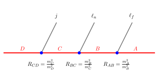
Figure 1: The typical cascade decay chain used in mass measurement studies. Here $D$, $C$, $B$ and $A$ are new BSM particles, while the corresponding SM decay products are: a QCD jet $j$, a “near” lepton $\ell_{n}^{\pm}$ and a “far” lepton $\ell_{f}^{\mp}$. This chain is quite common in SUSY, with the identification $D=\tilde{q}$, $C=\tilde{\chi}^{0}_{2}$, $B=\tilde{\ell}$ and $A=\tilde{\chi}^{0}_{1}$, where $\tilde{q}$ is a squark, $\tilde{\ell}$ is a slepton, and $\tilde{\chi}^{0}_{1}$ ($\tilde{\chi}^{0}_{2}$) is the first (second) lightest neutralino. Results for the masses of the new particles are often quoted in terms of the $D$ mass $m_{D}$ and the three dimensionless squared mass ratios $R_{CD}$, $R_{BC}$ and $R_{AB}$.

The main difficulty in the analysis of the decay chain of Fig. 1 stems from the fact that particle $A$, being a dark matter candidate, is invisible in the detector, hence its energy and momentum are not directly measured. This makes the problem of determining the masses and spins of the new particles $A$ through $D$ rather challenging. Over the last 20 years, a fairly large body of literature has been devoted to this problem. Among the different approaches which have been proposed, the classic method of kinematic endpoints is arguably the most popular and robust technique for mass determination. With this method, one studies the invariant mass distributions of different combinations of the visible decay products and attempts to locate their kinematic endpoints (generally in the presence of some background continuum). In the example of the decay chain in Fig. 1, one can form three 2-body invariant mass variables ($m_{j\ell_{n}}$, $m_{j\ell_{f}}$, and $m_{\ell\ell}$) and one 3-body invariant mass variable, $m_{j\ell\ell}$, so that the basic set of invariant mass variables is

$$\left\{m_{j\ell_{n}},m_{j\ell_{f}},m_{\ell\ell},m_{j\ell\ell}\right\}.$$ (1)

Ideally, one would like to study each of the variables (1) individually and obtain the corresponding kinematic endpoints $m_{j\ell_{n}}^{max}$, $m_{j\ell_{f}}^{max}$, $m_{\ell\ell}^{max}$, and $m_{j\ell\ell}^{max}$, which can be simply related to the unknown masses $\{m_{A},m_{B},m_{C},m_{D}\}$ by analytic expressions available in the literature (see, e.g., Allanach:2000kt ; Gjelsten:2004ki ; Burns:2009zi ). Unfortunately, the situation is not that simple, as it becomes muddled by various combinatorial ambiguities:

• Partitioning ambiguity. In general, in addition to the three visible objects from the decay chain in Fig. 1, there will be a number of additional objects in the event — the decay products from the other decay chain in the event, jets from initial state radiation, pile-up, etc. The question then becomes, how to select the correct objects $j$, $\ell_{n}$ and $\ell_{f}$ for the analysis variables (1). This is a really challenging problem, for which no universal solution exists, although several ideas have been tried, including the “hemisphere method” MP ; Matsumoto:2006ws , (a combination of) invariant mass and $M_{T2}$ cuts Rajaraman:2010hy ; Bai:2010hd ; Baringer:2011nh ; Choi:2011ys , and neural networks Shim:2014aua . In this paper, we will ignore the partitioning ambiguity and instead focus on the ordering ambiguity described next. Our assumption is justified in the case when particle $D$ is produced singly, or when $D$ is produced in association with the stable particle $A$, so that a second decay chain simply does not exist.

• Ordering ambiguity. Having selected the correct visible objects arising in a given decay chain, we still have to decide on the order in which they are emitted along the chain. For example, motivated by SUSY, in Fig. 1 one makes the specific assumption that the jet comes first, followed by the two leptons. However, even with this extra assumption, the ambiguity is not completely resolved, as we still do not know the exact ordering of the two leptons. In other words, we are not justified in using the labels “near” and “far” to denote the two leptons, which makes it impossible to study separately the distributions of $m_{j\ell_{n}}$ and $m_{j\ell_{f}}$ in the real experiment.

  Two possible ways out of this conundrum have been suggested. The standard approach Allanach:2000kt is to trade the variables $m_{j\ell_{n}}$ and $m_{j\ell_{f}}$ for their ordered cousins

  $$m_{j\ell(lo)} \equiv \min\left\{m_{j\ell_{n}},m_{j\ell_{f}}\right\},$$ (2)

  $$m_{j\ell(hi)} \equiv \max\left\{m_{j\ell_{n}},m_{j\ell_{f}}\right\}.$$ (3)

  Then, instead of the set (1), one can consider the alternative set of variables

  $$\left\{m_{j\ell(lo)},m_{j\ell(hi)},m_{\ell\ell},m_{j\ell\ell}\right\},$$ (4)

  measure their respective endpoints, and from those extract the physical mass spectrum Allanach:2000kt ; Gjelsten:2004ki ; Burns:2009zi . A more recent alternative approach Matchev:2009iw introduces new invariant mass variables which are symmetric functions of $m_{j\ell_{n}}$ and $m_{j\ell_{f}}$, thus avoiding the need to distinguish $\ell_{n}$ from $\ell_{f}$ on an event per event basis.

However, while both of these approaches are designed to address the ordering ambiguity problem, it is our view that they do not go far enough — in the sense that the assumption of the jet being the first emitted particle is still hardwired in the analysis from the very beginning. From the point of view of an experimenter whose duty is to perform unbiased measurements without theoretical prejudice, there is no compelling reason to make that assumption. One can easily construct theory models in which the jet is the second (or the third) visible particle in the diagram of Fig. 1. In order to account for such scenarios, one needs to further generalize the reordering in Eqs. (2,3) to include swapping the jet with one of the leptons. To be concrete, for the example of Fig. 1, we propose to further replace the two-body invariant mass variables $m_{j\ell(lo)}$, $m_{j\ell(hi)}$ and $m_{\ell\ell}$ from (4) with the three ordered variables

$$m_{(2,1)} \equiv {\max}_{1}\left\{m_{j\ell_{n}},m_{j\ell_{f}},m_{\ell\ell}\right\},$$ (5)

$$m_{(2,2)} \equiv {\max}_{2}\left\{m_{j\ell_{n}},m_{j\ell_{f}},m_{\ell\ell}\right\},$$ (6)

$$m_{(2,3)} \equiv {\max}_{3}\left\{m_{j\ell_{n}},m_{j\ell_{f}},m_{\ell\ell}\right\},$$ (7)

where we have used the function ${\max}_{r}$ to denote the $r$-th largest among a given set of elements. The variable set (4) is then replaced by

$$\left\{m_{(2,1)},m_{(2,2)},m_{(2,3)},m_{j\ell\ell}\right\},$$ (8)

whose kinematic endpoints can then be used to extract the physical spectrum. To this end, however, one would first need to derive the analytic formulas for these new endpoints in terms of the physical masses, and this will be one of the main goals of this paper.

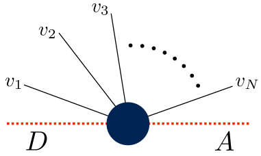
Figure 2: The generic decay of a heavy resonance $D$ to $N$ indistinguishable visible particles (solid black lines) and one invisible particle $A$ (red dashed line).

In summary, in this paper we propose to evade the ordering ambiguity problem by considering all possible partitions of the visible particles resulting from a given cascade decay chain, and then studying the kinematic endpoints of the corresponding sorted invariant mass variables. We shall try to keep our discussion as general as possible — for example, in defining the sorted invariant mass variables, we shall have in mind the generic diagram in Fig. 2 instead of the specific SUSY-inspired example of Fig. 1. In the case of Fig. 2, a heavy resonance $D$ decays to $N$ indistinguishable visible particles (denoted by solid black lines) and one invisible particle $A$ (denoted by a red dashed line). We first form the set

$${\cal S}_{n}^{N}\equiv\left\{m_{v_{i_{1}}v_{i_{2}}\ldots v_{i_{n}}}\right\}$$ (9)

of all possible $n$-body invariant mass combinations $m_{v_{i_{1}}v_{i_{2}}\ldots v_{i_{n}}}$ for a given $n\in\left[2,N\right]$. The total number $C^{N}_{n}$ of elements in the set ${\cal S}_{n}^{N}$ depends on the choice of $n$ and is given by the binomial coefficient

$$C^{N}_{n}=\begin{pmatrix}N\\ n\end{pmatrix}=\frac{N!}{n!(N-n)!}.$$ (10)

We can now uniquely and unambiguously label the members of the set ${\cal S}_{n}^{N}$ by defining sorted invariant mass variables in analogy to Eqs. (5-7):

$$m_{(n,r)}\equiv{\max}_{r}\left\{{\cal S}_{n}^{N}\right\}.$$ (11)

Using Eq. (10), it is easy to see that for a given $N$, there are a total of

$$\sum_{n=2}^{N}C^{N}_{n}=2^{N}-N-1$$ (12)

such variables. The physical meaning of the variable $m_{(n,r)}$ is that it is the $r$-th largest among all possible $n$-body invariant mass combinations of visible particles in Fig. 2. From the general definition (11) it is easy to make contact with the previously considered $N=3$ case of Fig. 1: in the notation of (11), the variable set (8) corresponds to

$$\left\{m_{(2,1)},m_{(2,2)},m_{(2,3)},m_{(3,1)}\right\}.$$ (13)

In introducing the more general variables (11) we are motivated by several factors:

1. Often the visible particles in the cascade decay are indistinguishable, e.g. they are all QCD jets. This can easily be the case even with the SUSY example of Fig. 1, whenever the second-lightest neutralino (particle $C$) decays predominantly hadronically to 2 jets and the lightest neutralino (particle $A$). Another well motivated SUSY example is a squark-gluino-neutralino decay chain where again all three visible particles are jets. In such scenarios, a priori there is no way to single out any particular jet, and the set (13) is the only one which makes physics sense.

2. In a purely off-shell scenario, where particle $D$ decays directly to particle $A$ plus $N$ visible particles, it is not possible to assign any specific order to the decay products, even if they are distinguishable experimentally.

3. Even when the decay of particle $D$ proceeds through intermediate narrow resonances, so that the visible decay products are emitted in some well-defined order, this true order is unknown to the experimentalist, and can only be hypothesized. In general, alternative theory models, with alternative orderings of the same final state particles, are also possible. Therefore, assuming a specific ordering throughout the analysis is dangerous and may lead to wrong conclusions.

4. Finally, by staying clear of any theory bias, and considering the most general case of Fig. 2, we will be able to derive (see Section 2 below) the necessary relations which must be obeyed by the kinematic endpoints of the variables (11) in the case of a pure off-shell decay (i.e., with no intermediate resonances). Any observed deviations from those predictions will signal the presence of new particles in addition to the mother $D$ and daughter $A$. Furthermore, as illustrated in Fig. 26 below, the measured relations among the kinematic endpoints are indicative of the particular on-shell event topology at hand.

In this paper we begin the investigation of the mathematical properties of the variables (11), and, in particular, their kinematic endpoints. In Section 2 we focus on the general case of an off-shell $1\to N+1$ decay as depicted in Fig. 2. We derive the formulas for the kinematic endpoints of the sorted invariant mass variables (11) in terms of the relevant physical mass parameter, the mass difference $m_{D}-m_{A}$. For $N>2$, the number of variables given by (12) already exceeds the number of input parameters, which implies certain specific relations among the measured kinematic endpoints. Among the main results of Section 2 is the derivation of these relations, as they provide a stringent test of the offshellness of the decay topology.

Having dealt with the general case of arbitrary $N$ in Section 2, in the following sections we return to the SUSY-motivated case of $N=3$. We shall similarly study the dependence of the sorted invariant mass endpoints on the physical mass parameters, in the presence of intermediate on-shell resonances. The relevant special cases are discussed in Sections 3, 4 and 5. Section 6 is reserved for our summary and conclusions.

2 The pure off-shell case of $(N+1)$-body decay

Consider the decay of a heavy resonance $D$ into $N$ massless visible particles and one massive invisible particle $A$, as shown in Fig. 2:

$$D\rightarrow v_{1}v_{2}\cdots v_{N}A.$$ (14)

In this section we shall assume that the decay (14) proceeds in one step, i.e., exactly as depicted in Fig. 2. In other words, any virtual particles hiding behind the circular blob in Fig. 2 are sufficiently heavy and can be integrated out to give rise to an effective contact interaction as shown in the figure.

As mentioned in the Introduction, we treat all visible particles in the final state as indistinguishable, so that we do not know a priori the sequence in which the visible particles are emitted. This motivates us to consider the sorted invariant mass variables $m_{(n,r)}$ defined in Eq. (11). In what follows, we shall refer to the first index $n$ as the “order” of the variable, while the second index $r$ will denote its “rank”. Obviously, the order $n$ can be chosen to be any integer from 2 to $N$; for completeness we shall consider all possible values of $n$, i.e., we shall construct two-body, three-body, etc. invariant masses of visible particles. For a given order $n$, the rank $r$ then takes values from 1 to $C^{N}_{n}$.

Our main goal in this section is to provide the analytic expressions for the kinematic endpoints $m_{(n,r)}^{max}$ in terms of the physical masses $m_{D}$ and $m_{A}$. In all results below, we shall always factor out the parent mass $m_{D}$ and write the formulas in terms of the dimensionless squared mass ratios

$$R_{ij}\equiv\frac{m_{i}^{2}}{m_{j}^{2}},\;\;\;\{i,j\}\in\{D,C,B,A\},$$ (15)

where by assumption the particle masses obey the hierarchy

$$m_{D}>m_{C}>m_{B}>m_{A}.$$ (16)

In the case of the pure off-shell process (14), the only two masses entering the problem are $m_{D}$ and $m_{A}$, thus our results will be functions of $R_{AD}<1$.

2.1 Invariant masses of order $n=2$

We first discuss the sorted invariant masses of order 2 (i.e., the two-body invariant masses), for which a useful sum rule can be derived as follows. Using $4$-momentum conservation for the reaction (14)

$$p_{D}=p_{1}+\cdots+p_{N}+p_{A},$$ (17)

we can write

$$(p_{D}-p_{A})^{2}=(p_{1}+\cdots+p_{N})^{2}=\sum_{i=1}^{N}p_{i}^{2}+2\sum_{\begin{subarray}{c}i,j=1\\ i<j\end{subarray}}^{N}p_{i}\cdot p_{j},$$ (18)

Since the visible particles are assumed massless, $p_{i}^{2}=0$, and furthermore, $2p_{i}\cdot p_{j}$ is simply $(p_{i}+p_{j})^{2}=m_{ij}^{2}$ so that the above relation can be rewritten as

$$(p_{D}-p_{A})^{2}=\sum_{r=1}^{C_{2}^{N}}m_{(2,r)}^{2}.$$ (19)

The left-hand side in this equation may be interpreted as the “total available invariant mass squared” which is allocated to $m_{(2,r)}^{2}$’s in a given event. Since Eq. (19) is Lorentz-invariant, we can evaluate its left-hand side in any frame. It is convenient to choose the rest frame of particle $D$, where

$$(p_{D}-p_{A})^{2}=m_{D}^{2}+m_{A}^{2}-2m_{D}E_{A}.$$ (20)

We are interested in kinematic endpoints, i.e., the cases in which a particular variable $m_{(2,r)}$ is maximized. Eq. (19) suggests that in order to maximize an individual variable $m_{(2,r)}$, we must necessarily maximize the total quantity (20) as well. It is easy to see that (20) is maximized when $A$ is produced at rest and its energy $E_{A}=m_{A}$. We therefore conclude that for an event which yields a kinematic endpoint of $m_{(2,r)}$ for some value of $r$, the following sum rule holds

$$\sum_{r}m_{(2,r)}^{2}=(m_{D}-m_{A})^{2}.$$ (21)

We are now in position to derive the formulas for the kinematic endpoints $m_{(2,r)}^{max}$ for various $r$.

Rank $r=1$. The largest possible value of $m_{(2,1)}$ is obtained when all other invariant mass combinations are vanishing, i.e., for events in which

$$m_{(2,1)}=m_{(2,1)}^{max}\quad{\rm and}\quad m_{(2,r)}=0,\quad{\rm for}\quad r=2,\ldots,C^{N}_{2}.$$ (22)

The momentum configuration of such an event is shown in Fig. 3 — two of the visible particles are exactly back-to-back, while the remaining visible particles, together with the invisible particle $A$, are all at rest. The $m_{(2,1)}^{max}$ endpoint is now obtained by substituting (22) into (21):

$$m_{(2,1)}^{\max}=m_{D}-m_{A}=m_{D}\,(1-\sqrt{R_{AD}}).$$ (23)

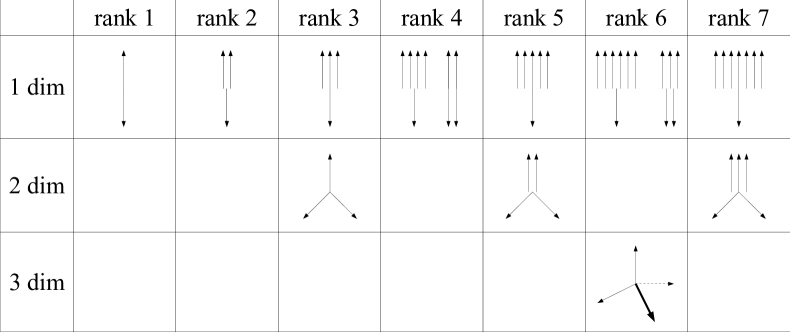
Figure 3: Possible geometric orientations of the visible particle momenta in the extreme events corresponding to the kinematic endpoints of the $m_{(2,r)}$ variables for $r\leq 7$. The lengths of the arrows are not indicative of the relative magnitudes of the momenta. The remaining visible particles not depicted by arrows are taken to be at rest. The configurations in the first row are collinear, the configurations in the second row are planar, while the configurations in the third row are three-dimensional.

Rank $r=2$. According to Eq. (21), in order to maximize $m_{(2,2)}$, we need to minimize both $m_{(2,1)}$ and $m_{(2,r)}$ for $r\geq 3$. However, by definition $m_{(2,1)}$ cannot be less than $m_{(2,2)}$, thus for events giving the largest possible value of $m_{(2,2)}$ we expect to have

$$m_{(2,1)}=m_{(2,2)}=m_{(2,2)}^{max}\quad{\rm and}\quad m_{(2,r)}=0,\quad{\rm for}\quad r=3,\ldots,C^{N}_{2}.$$ (24)

The momentum configurations of such events are also collinear, as shown in Fig. 3. Now there are three visible particles with non-zero momenta, two of them having equal momenta and recoiling against the third. From (24) and (21) we obtain

$$m_{(2,2)}^{\max}=\frac{1}{\sqrt{2}}\,(m_{D}-m_{A})=\frac{1}{\sqrt{2}}\,m_{D}\,(1-\sqrt{R_{AD}}).$$ (25)

Higher ranks ($r>2$). Proceeding analogously, one might naïvely expect that for an arbitrary rank $r$, Eqs. (23) and (25) generalize to

$$m_{(2,r)}^{\max}\stackrel{{\scriptstyle?}}{{=}}\frac{1}{\sqrt{r}}\,(m_{D}-m_{A})=\frac{1}{\sqrt{r}}\,m_{D}\,(1-\sqrt{R_{AD}}).$$ (26)

However, one has to be careful to check whether physical momentum configurations exist such that

$$m_{(2,1)}=m_{(2,2)}=\ldots=m_{(2,r)}=m_{(2,r)}^{max}\quad{\rm and}\quad m_{(2,i)}=0,\quad{\rm for}\quad i=r+1,\ldots,C^{N}_{2}.$$ (27)

This check is not aways trivial. As a concrete example, consider the rank 10 variable $m_{(2,10)}$ in the case of $N=5$ total visible particles. It is not difficult to see that in three spatial dimensions, there are no allowed momentum configurations which would give the required case with $m_{(2,1)}=m_{(2,2)}=\cdots=m_{(2,10)}$. As a result, in this case the conjectured endpoint

$$m_{(2,10)}^{\max}\stackrel{{\scriptstyle?}}{{=}}\frac{1}{\sqrt{10}}\,(m_{D}-m_{A})$$ (28)

will not be saturated, and the true endpoint will appear at slightly lower values of $m_{(2,10)}$. However, in such situations where the general formula (26) happens to overestimate the kinematic endpoint, it is nevertheless possible to obtain the correct answer by inspecting the candidate momentum configurations for the visible particles in the rest frame of the mother particle $D$.

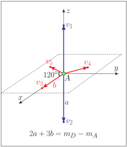
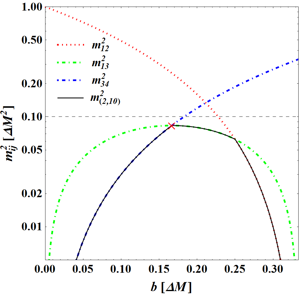
Figure 4: Left: a candidate momentum configuration of the $N=5$ visible particles in the $D$ rest frame for an event contributing to the $m_{(2,10)}$ endpoint. Each of the blue (red) momentum vectors has magnitude $a$ ($b$), and the vectors themselves are arranged in the shape of a triangular bipyramid. Energy conservation implies the relation $2a+3b=m_{D}-m_{A}$. Right: The three different two-body invariant masses squared as a function of $b$ (measured in units of $\Delta M=m_{D}-m_{A}$): $m_{12}^{2}$ (red dotted line); $m_{13}^{2}=m_{14}^{2}=m_{15}^{2}=m_{23}^{2}=m_{24}^{2}=m_{25}^{2}$ (green dot-dashed line); $m_{34}^{2}=m_{45}^{2}=m_{35}^{2}$ (blue dot-dashed line). The black solid line corresponds to $m_{(2,10)}^{2}$, which peaks at $b=\Delta M/6$, leading to the exact bound (29).

Let us illustrate the procedure with the above example of $N=5$ visible particles, and try to obtain the exact upper bound for $m_{(2,10)}$. For this purpose, we look for momentum configurations, in which the visible particles $v_{i}$ are maximally “spread out” in the rest frame of the mother particle $D$, while the massive invisible particle $A$ is still at rest. The main idea is that the desired configurations will exhibit a certain level of symmetry, as demonstrated in Figs. 4 and 5. The left panels in the figures depict the momentum configurations of the visible particles in the $D$ rest frame, whereby momenta in blue (red) have the same magnitude $a$ ($b$).

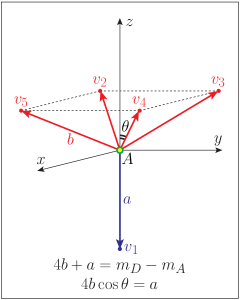
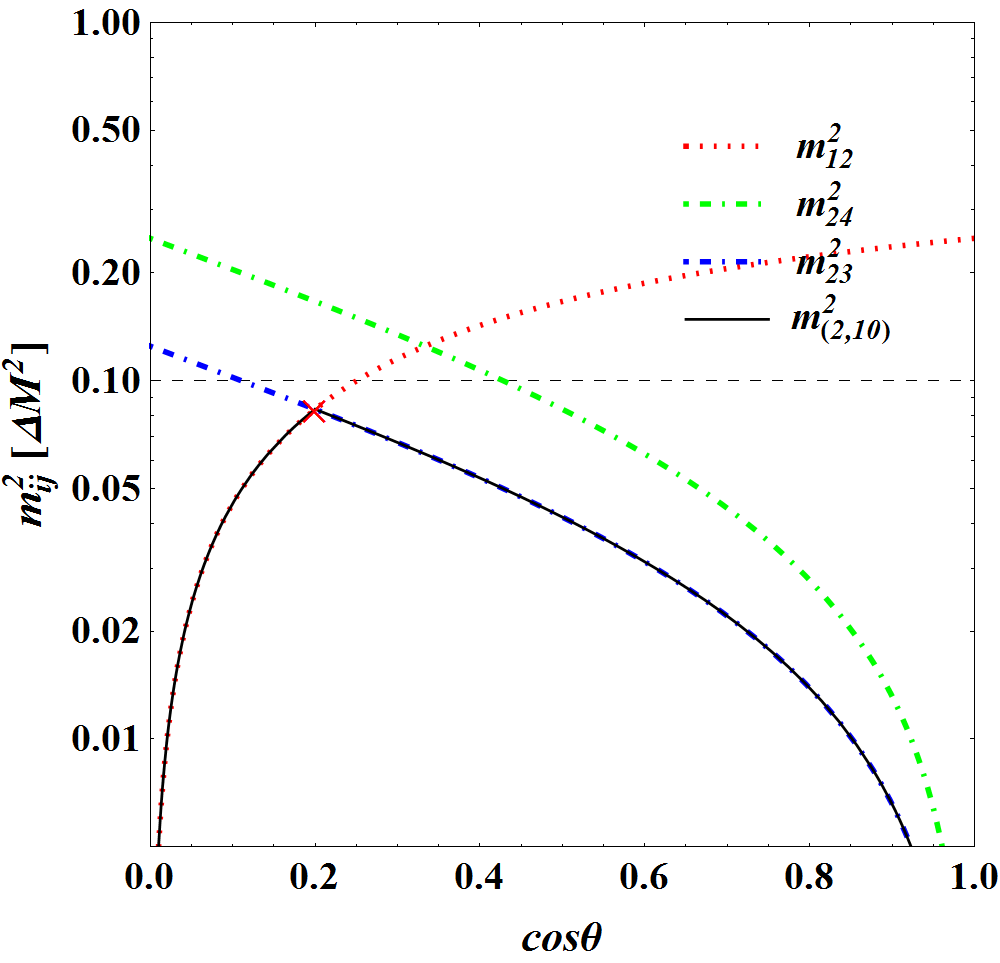
Figure 5: The same as Fig. 4, but for an alternative, pyramid-like, momentum configuration. Energy conservation implies $4b+a=m_{D}-m_{A}$, while momentum conservation along $z$ requires $4b\cos\theta=a$, leaving only one independent degree of freedom, which in the right panel is chosen as $\cos\theta$. In this configuration, we have $m_{12}^{2}=m_{13}^{2}=m_{14}^{2}=m_{15}^{2}$ (red dotted line); $m_{24}^{2}=m_{35}^{2}$ (green dot-dashed line); and $m_{23}^{2}=m_{34}^{2}=m_{45}^{2}=m_{25}^{2}$ (blue dot-dashed line). The maximal value of $m_{(2,10)}^{2}$ is obtained for $\cos\theta=1/12$, once again leading to the bound (29).

Energy and momentum conservation imply certain relations among the magnitudes and the relative orientation of the momentum vectors as shown. In each case, the remaining sole degree of freedom can be varied in order to find the maximum of the ranked variable $m_{(2,10)}$ as

$$N=5:\quad m_{(2,10)}^{\max}=\frac{1}{\sqrt{12}}\,(m_{D}-m_{A}).$$ (29)

As expected, this bound is tighter than the naïve expectation (28).

One can similarly analyze the case of $N=6$, where we find three competing momentum configurations: a pentagonal pyramid, a square bipyramid, and a triangular prism wedge. The latter provides the true maximum value of the $m_{(2,15)}$ ranked variable:

$$N=6:\quad m_{(2,15)}^{\max}=\sqrt{\frac{253}{4536}}\,(m_{D}-m_{A})<\frac{1}{\sqrt{15}}\,(m_{D}-m_{A}),$$ (30)

while the bipyramid-like configuration provides the maximum of $m_{(2,14)}$:

$$N=6:\quad m_{(2,14)}^{\max}=\frac{1}{\sqrt{9\sqrt{3}}}\,(m_{D}-m_{A})<\frac{1}{\sqrt{14}}\,(m_{D}-m_{A}).$$ (31)

In summary, for large enough ranks $r$ (as in the examples just considered), the upper bound provided by Eq. (26) will not be saturated, and the kinematic endpoint $m_{(2,r)}^{max}$ will be found at somewhat lower values. The lowest value of $r$ at which the prediction (26) begins to deviate from the true answer, in general depends on the number of visible particles $N$. We have checked that Eq. (26) can be trusted up to the following rank

$$r^{\prime}=\left\{\begin{array}[]{l}6k^{2}\hskip 71.13188pt\hbox{for }N=4k,\\ 6k^{2}+3k\hskip 45.52458pt\hbox{for }N=4k+1,\\ 6k^{2}+6k+1\hskip 28.45274pt\hbox{for }N=4k+2,\\ 6k^{2}+9k+3\hskip 28.45274pt\hbox{for }N=4k+3,\end{array}\right.$$ (32)

where $k$ is a non-zero integer. For ranks $r$ higher than the rank $r^{\prime}$ given by Eq. (32), the expression (26) provides simply an upper bound on the kinematic endpoint $m_{(2,r)}^{\max}$.

2.2 Invariant masses of order $n>2$

Once we consider more than two particles at a time, the situation becomes more complicated. As a concrete example, let us take $N=4$ visible particles and investigate the third order ($n=3$) variables $m_{123}$, $m_{124}$, $m_{134}$, and $m_{234}$. Momentum conservation (17) now leads to the following relation (compare to Eqs. (18) and (19))

$$\sum_{r=1}^{C^{4}_{3}=4}m_{(3,r)}^{2}=2\times 2\sum_{\begin{subarray}{c}i,j=1\\ i<j\end{subarray}}^{N=4}p_{i}\cdot p_{j}=2\,(p_{D}-p_{A})^{2}.$$ (33)

As before, the kinematic endpoints are attained when particle $A$ is produced at rest in the rest frame of particle $D$, so that the above equation reduces to the following analogue of Eq. (21)

$$\sum_{r=1}^{4}m_{(3,r)}^{2}=2\,(m_{D}-m_{A})^{2}=2\,m_{D}^{2}\,(1-\sqrt{R_{AD}})^{2}.$$ (34)

Rank $r=1$. There are two types of events which determine the endpoint of $m_{(3,1)}$. The first type of events have two visible particles moving back-to-back in the $D$ rest frame, while the other two visible particles are at rest. In this configuration, we have

$$m_{(3,1)}=m_{(3,2)}=m_{(3,1)}^{max}\left(=m_{(3,2)}^{max}\right)\quad{\rm and}\quad m_{(3,3)}=m_{(3,4)}=0.$$ (35)

In the other configuration, three visible particles with equal energies are moving in a plane at $120^{\circ}$ with respect to each other, while the fourth visible particle is at rest. This in turn implies that

$$m_{(3,1)}=m_{(3,1)}^{max}\quad{\rm and}\quad m_{(3,2)}=m_{(3,3)}=m_{(3,4)}=\frac{1}{\sqrt{3}}\,m_{(3,1)}.$$ (36)

Using either Eq. (35) or Eq. (36) in the sum rule (34), we find

$$m_{(3,1)}^{\max}=m_{D}-m_{A}=m_{D}\,(1-\sqrt{R_{AD}}).$$ (37)

Rank $r=2$. The maximal value for $m_{(3,2)}$ is obtained for the momentum configuration given by (35), thus the endpoint is the same as (37):

$$m_{(3,2)}^{\max}=m_{D}-m_{A}=m_{D}\,(1-\sqrt{R_{AD}}).$$ (38)

Ranks $r=3$ and $r=4$. For the third- and fourth-ranked three-body invariant masses, we apply the reasoning from Section 2.1 to obtain similar expressions. Our final answer for the case of $N=4$ visible particles is thus

$$m_{(3,r)}^{\max}=\left\{\begin{array}[]{l}m_{D}\,(1-\sqrt{R_{AD}})\hskip 56.9055pt\hbox{for }r\leq 2\\ \\ \sqrt{\frac{2}{r}}\,m_{D}\,(1-\sqrt{R_{AD}})\hskip 39.83368pt\hbox{for }r\geq 2.\end{array}\right.$$ (39)

Having worked out this simple example, we can now generalize (39) to higher orders $n>3$. Suppose that there are $N$ visible particles as usual, and we consider invariant mass combinations of order $n$. Fixing two visible particles, say $i$ and $j$, the term $2p_{i}\cdot p_{j}$ appears in $C^{N-2}_{n-2}$ invariant mass variables out of the total possible number $C^{N}_{n}$. We have already seen that summing $2p_{i}\cdot p_{j}$ over all possible pairs of indices $i$ and $j$ is related to a sum over all possible $n$-body invariant mass combinations:

$$\sum_{r}m_{(n,r)}^{2}=C^{N-2}_{n-2}\times(p_{D}-p_{A})^{2}.$$ (40)

The kinematic endpoints that we are interested in are obtained when the right-hand-side of this relation is maximized (by virtue of particle $A$ being at rest in the $D$ rest frame):

$$\sum_{r}m_{(n,r)}^{2}=C^{N-2}_{n-2}\times(m_{D}-m_{A})^{2}.$$ (41)

Retracing the steps which led to Eq. (39), we get

$$m_{(n,r)}^{\max}=\left\{\begin{array}[]{l}m_{D}\,(1-\sqrt{R_{AD}})\hskip 56.9055pt\hbox{for }r\leq C^{N-2}_{n-2},\\ \\ \sqrt{\frac{C^{N-2}_{n-2}}{r}}\,m_{D}\,(1-\sqrt{R_{AD}})\hskip 22.76228pt\hbox{for }r\geq C^{N-2}_{n-2}.\end{array}\right.$$ (42)

As already discussed at the end of Section 2.1, this formula provides the exact maximum only up to some rank, i.e., for sufficiently high ranks, it only gives an upper bound. However, even with such high ranks, the true endpoint will still be proportional to the mass difference $m_{D}-m_{A}=m_{D}(1-\sqrt{R_{AD}})$, only with a pre-factor which is somewhat smaller than $\sqrt{\frac{C^{N-2}_{n-2}}{r}}$.

2.3 Testing for off-shellness

Armed with the general result (42), one can now design a specific test to verify that the decay topology is indeed a purely off-shell one as hypothesized in Fig. 2. The main observation is that in a purely off-shell topology the kinematic endpoints of all invariant mass variables are functions of a single degree of freedom, $m_{D}-m_{A}$. This implies certain relationships, or “sum rules” for short, among the kinematic endpoints. These sum rules are quantitatively predicted by Eq. (42). Note that by introducing the sorted variables (11), we are considering the largest possible number of invariant mass variables, and therefore we obtain the largest possible number of sum rules.

For illustration, let us consider the simplest case of $N=3$ visible particles, as in the SUSY-like decay chain of Fig. 1. There are $2^{3}-3-1=4$ sorted variables given by (13), and one unknown degree of freedom, $m_{D}-m_{A}$, which leaves us with three sum rules. Therefore, if this were a purely off-shell process, the following relations must hold

$$\frac{m_{(3,1)}^{max}}{m_{(2,1)}^{max}} = 1,$$ (43)

$$\frac{m_{(2,2)}^{max}}{m_{(2,1)}^{max}} = \frac{1}{\sqrt{2}},$$ (44)

$$\frac{m_{(2,3)}^{max}}{m_{(2,1)}^{max}} = \frac{1}{\sqrt{3}}.$$ (45)

The violation of one or more of these relations would indicate one of two things — either the presence of intermediate on-shell resonances, or some sort of momentum-dependent couplings (form-factors).

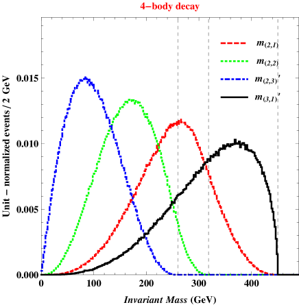
Figure 6: The distributions of the sorted variables $m_{(2,1)}$ (red dashed line), $m_{(2,2)}$ (green dotted line), $m_{(2,3)}$ (blue dot-dashed line) and $m_{(3,1)}$ (black solid line), for a 4-body decay ($N=3$ in Eq. (14)) with $m_{D}=500$ GeV and $m_{A}=50$ GeV. The kinematic endpoints predicted by (42) are marked with the vertical black dashed lines and are located at 450 GeV, 318 GeV, 260 GeV and 450 GeV, correspondingly.

The relationships (43-45) are illustrated in Fig. 6. We consider a four-body pure off-shell decay, i.e., the reaction (14) with $N=3$, and plot the distributions of the four relevant sorted invariant mass variables: $m_{(2,1)}$ (red dashed line), $m_{(2,2)}$ (green dotted line), $m_{(2,3)}$ (blue dot-dashed line) and $m_{(3,1)}$ (black solid line). Eq. (42) predicts that their respective endpoints will be located at 450 GeV, 318 GeV, 260 GeV and 450 GeV. Fig. 6 shows that the endpoint structure for $m_{(3,1)}$ can be identified very well and the value of the endpoint clearly agrees with the theoretical prediction. The two-body invariant mass distributions for $m_{(2,i)}$ also saturate the theoretical bounds (42). However, we note that those distributions are relatively shallow near their upper kinematic endpoints BK ; Cho:2012er ; Giudice:2011ib , which might make the experimental extraction of those endpoints rather challenging Lester:2006yw .

3 The pure on-shell decay topology with $N=3$ visible particles

Having considered the purely off-shell case in complete generality in the previous section, we now turn our attention to decay topologies with intermediate on-shell resonances. Unfortunately, the general analysis for an arbitrary number of visible particles $N$ gets quite complicated, which is why in this and the subsequent sections we shall limit our discussion to the most interesting case of $N=3$, as in the SUSY-like decay chain from Fig. 1. In particular, we shall focus on the four possibilities depicted in Fig. 7.

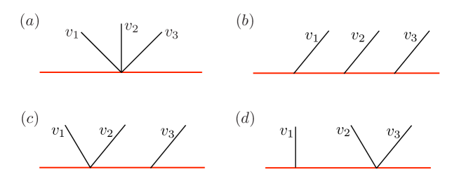
Figure 7: The four possible decay topologies with $N=3$ massless visible particles $v_{1}$, $v_{2}$ and $v_{3}$.

The event topology of Fig. 7(a) is simply a special case of a purely off-shell decay already considered in the previous section. The event topology of Fig. 7(b) is the typical SUSY scenario from Fig. 1 and will be the main subject of this section. It involves a sequence of three 2-body decays, where each decay produces one visible particle. We shall sometimes refer to the diagram of Fig. 7(b) as a $(1,1,1)$ decay topology. The event topologies of Figs. 7(c) and 7(d) are “hybrid” event topologies in the sense that they involve both a two-body and a three-body decay. Correspondingly, the diagram of Fig. 7(c) will be referred to as a $(2,1)$ topology and will be studied in the next Section 4, while the diagram of Fig. 7(d) will be labelled as a $(1,2)$ topology and will be considered in Section 5.

3.1 The phase space structure of the $(1,1,1)$ decay topology

Before discussing the properties of the ranked variables (11), it is instructive to review the properties of the allowed phase space in terms of the original variables (1) Costanzo:2009mq ; CLTASI . The relevant kinematic variables for the $(1,1,1)$ decay of a heavy particle $D$ into an invisible particle $A$ and visible particles $v_{1}$, $v_{2}$ and $v_{3}$ are depicted in Fig. 8. We note that the $(1,1,1)$ decay is most conveniently described in the rest frame of particle $C$ as shown in Fig. 8(b). Naïvely, the total number of degrees of freedom is four, but one of them (here the overall azimuthal angle $\beta$) can be neglected taking into account the azimuthal symmetry of this phase space. The remaining three degrees of freedom are: the polar angle $\alpha$ of the momentum of $v_{2}$ with respect to the direction of $v_{1}$, the polar angle $\theta$ of the momentum of $v_{3}$ with respect to the direction of $C$ in the rest frame of particle $B$, and the azimuthal angle $\phi$ between the planes defined by $(v_{1},v_{2})$ and $(v_{2},v_{3})$ in the $C$ rest frame.

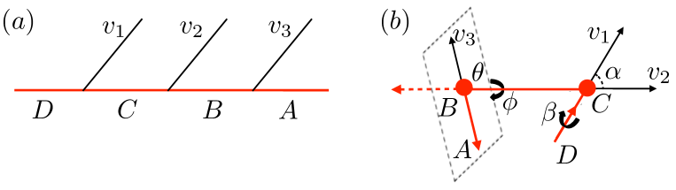
Figure 8: (a) The $(1,1,1)$ decay topology of a heavy particle $D$ into a lighter particle $A$ and three massless visible particles $v_{1}$, $v_{2}$ and $v_{3}$. (b) The relevant kinematic variables: $\alpha$ is the angle between the momenta of $v_{1}$ and $v_{2}$ in the rest frame of particle $C$, $\theta$ is the polar angle of the $v_{3}$ momentum with respect to the direction of $C$ in the $B$ rest frame, and $\phi$ is the azimuthal angle between the planes defined by the momenta of a) $v_{1}$ and $v_{2}$ and b) $v_{2}$ and $v_{3}$, in the $C$ rest frame.

This phase space can be equivalently described in terms of the invariant mass variables

$$\left\{m_{v_{1}v_{2}},m_{v_{1}v_{3}},m_{v_{2}v_{3}}\right\}.$$ (46)

However, to simplify notation, from here on we shall work with the dimensionless variables

$$x \equiv \frac{m^{2}_{v_{2}v_{3}}}{m_{D}^{2}}=\frac{(p_{2}+p_{3})^{2}}{m_{D}^{2}},$$ (47)

$$y \equiv \frac{m^{2}_{v_{1}v_{2}}}{m_{D}^{2}}=\frac{(p_{1}+p_{2})^{2}}{m_{D}^{2}},$$ (48)

$$z \equiv \frac{m^{2}_{v_{1}v_{3}}}{m_{D}^{2}}=\frac{(p_{1}+p_{3})^{2}}{m_{D}^{2}},$$ (49)

instead of the dimensionful set (46). In terms of the SUSY-like decay chain of Fig. 1, the variable $x$ corresponds to $m^{2}_{\ell\ell}$, the variable $y$ is the analogue of $m^{2}_{j\ell_{n}}$, while $z$ represents $m^{2}_{j\ell_{f}}$.

The three angular degrees of freedom $\theta$, $\alpha$ and $\phi$ from Fig. 8(b) can be mapped to the three dimensionless invariant mass variables (47-49) as follows:

$$x = \frac{x_{0}}{2}\left(1-\cos\theta\right),$$ (50)

$$y = \frac{y_{0}}{2}\left(1-\cos\alpha\right),$$ (51)

$$z = \frac{z_{0}\,e^{-\eta}}{2}\left\{\cosh\eta-\cos\theta\sinh\eta-\cos\alpha(\cos\theta\cosh\eta-\sinh\eta)-\cos\phi\sin\theta\sin\alpha\right\},~{}~{}~{}$$ (52)

where

$$x_{0} \equiv x_{max}=R_{CD}(1-R_{AB})(1-R_{BC}),$$ (53)

$$y_{0} \equiv y_{max}=(1-R_{BC})(1-R_{CD}),$$ (54)

$$z_{0} \equiv z_{max}=(1-R_{AB})(1-R_{CD}),$$ (55)

and

$$\eta\equiv\ln\left(\frac{m_{C}}{m_{B}}\right).$$ (56)

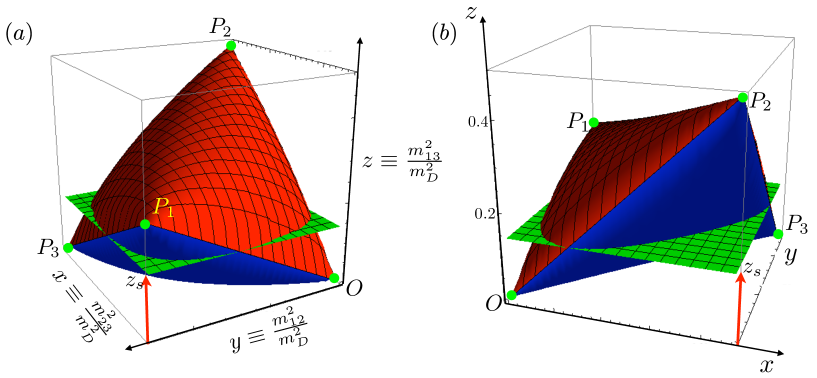
Figure 9: Two different views of the allowed phase space for a $(1,1,1)$ cascade decay chain, in terms of the dimensionless variables (47-49). The boundary surface is made of two separate sheets — the top one, colored red, is given by Eq. (57), while the bottom (blue) sheet is given by Eq. (58). The three points $\left\{P_{1},\,P_{2},\,P_{3}\right\}$ determine the shape of the surface. In order to study the ranked invariant mass distributions, we perform a CT-like scan at a fixed $z$ value $z_{s}$, as shown by the green plane. For this illustration, the mass spectrum has been chosen as $\left(m_{D},m_{C},m_{B},m_{A}\right)=\left(1000,700,500,100\right)$ GeV.

The allowed phase space spanned by (50-52) is shown in Fig. 9. Its shape has been likened to that of a samosa CLTASI and can be parametrized by two functions, $z^{+}(x,y)$ for the top surface (colored in red) and $z^{-}(x,y)$ for the bottom surface (colored in blue). In order to find the explicit form of $z^{\pm}(x,y)$, we note that the angle $\phi$ enters only the definition of $z$ in Eq. (49). Thus the extreme values of $z$ (for a fixed $x$ and $y$) are found for the extreme values of $\phi$, namely, $\phi=0$ and $\phi=\pi$ Costanzo:2009mq :

$$z^{+}(x,y) = z_{0}\left[\sqrt{\frac{x}{x_{0}}\left(1-\frac{y}{y_{0}}\right)}+e^{-\eta}\sqrt{\frac{y}{y_{0}}\left(1-\frac{x}{x_{0}}\right)}\right]^{2}\textrm{ for }\phi=\pi,$$ (57)

$$z^{-}(x,y) = z_{0}\left[\sqrt{\frac{x}{x_{0}}\left(1-\frac{y}{y_{0}}\right)}-e^{-\eta}\sqrt{\frac{y}{y_{0}}\left(1-\frac{x}{x_{0}}\right)}\right]^{2}\textrm{ for }\phi=0.$$ (58)

The exact shape of the “samosa” is determined by the location of the four “corner points” which in Fig. 9 are denoted as $\{O,\,P_{1},\,P_{2},\,P_{3}\}$

$$(\theta=0,\alpha=0) \rightarrow O=\left(0,\,0,\,0\right),$$ (59)

$$(\theta=0,\alpha=\pi) \rightarrow P_{1}=\left(0,\,y_{0},\,e^{-2\eta}\,z_{0}\right)\equiv(0,y_{0},z_{c}),$$ (60)

$$(\theta=\pi,\alpha=0) \rightarrow P_{2}=\left(x_{0},\,0,\,z_{0}\right),$$ (61)

$$(\theta=\pi,\alpha=\pi) \rightarrow P_{3}=\left(x_{0},\,y_{0},\,0\right).$$ (62)

3.2 Computer tomography of the allowed phase space

In order to analyze the allowed phase space from Fig. 9 in terms of the sorted variables (11), we need to rank the variables $x$, $y$ and $z$ among themselves. We do this by performing a computerized tomography (CT) scan in which the relevant cross sectional CT images are obtained at a fixed value $z=z_{s}$ along the $z$-axis (see the green plane in Fig. 9). In this CT scan process the point $P_{1}$ plays a special role because it divides the obtained images into two groups. Whenever the scan image is taken “below” $P_{1}$, i.e., at a value of $z_{s}$ smaller than the $z$ component of $P_{1}$

$$z_{c}\equiv e^{-2\eta}\,z_{0}=z_{0}\,R_{BC},$$ (63)

the boundary of the image consists of two segments obtained from setting $z^{+}(x,y)=z_{s}$, interspersed with another two segments given by $z^{-}(x,y)=z_{s}$ (see Fig. 9). On the other hand, when the image is taken “above” $P_{1}$, i.e., when $z_{s}>z_{c}$, the corresponding image boundary is made up of only one segment from each surface (top and bottom).

The basic procedure of ranking $x$, $y$ and $z$ with the CT scan method is the following. For a fixed $z=z_{s}$, the intersection of the green plane shown in Fig. 9 with the interior of the samosa determines the allowed values $x(z_{s})$ and $y(z_{s})$ at this particular value of $z=z_{s}$. We then sort $x(z_{s})$ and $y(z_{s})$ and find their respective maxima:

$$r_{1}\equiv\max\left\{\max\left[x(z_{s}),\;y(z_{s})\right]\right\},\quad r_{2}\equiv\max\left\{\min\left[x(z_{s}),\;y(z_{s})\right]\right\}.$$ (64)

Once this is done, we need to compare the thus obtained values of $r_{1}$ and $r_{2}$ to the value of $z$, so we sort again $\{r_{1},r_{2},z_{s}\}$ by magnitude for all possible $r_{1}$ and $r_{2}$ to obtain the “local” maxima of the sorted invariant masses at a given $z_{s}$:

$$\left.\left(m_{(2,r)}^{\max}\right)^{2}\right|_{z_{s}}=m_{D}^{2}\cdot\max_{r_{1},r_{2}}{}_{r}\left[r_{1},r_{2},z_{s}\right].$$ (65)

Finally, we find the “global” maxima of the sorted invariant mass variables by maximizing (65) for all allowed $z_{s}$:

$$m_{(2,\text{r})}^{\max}=\max_{z_{s}}\left\{\left.m_{(2,\text{r})}^{\max}\right|_{z_{s}}\right\}.$$ (66)

In evaluating $r_{2}$, it is convenient to fold the $(x,y)$ plane along the $x=y$ line Burns:2009zi . This motivates us to treat separately the cases of $x_{0}<y_{0}$ and $x_{0}\geq y_{0}$.

3.2.1 CT scans for the case of $x_{0}<y_{0}$

We first discuss the case of $x_{0}<y_{0}$, i.e., when the range of possible $y$ values is larger than the range of possible $x$ values. According to Eqs. (53) and (54), this occurs for mass spectra obeying the relation

$$x_{0}<y_{0}\Longleftrightarrow R_{CD}<\frac{1}{2-R_{AB}}.$$ (67)

Fig. 10 shows the eight characteristic shapes of the CT images obtained at different fixed values of $z_{s}$.

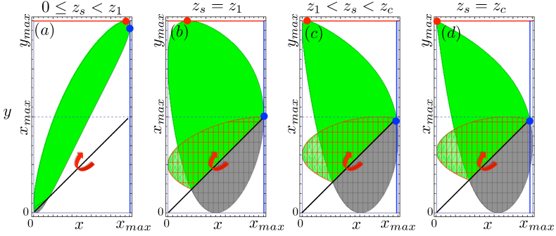
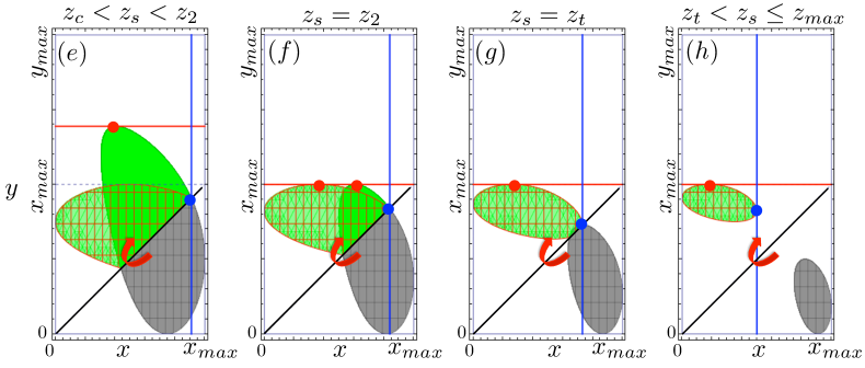
Figure 10: For the case of $x_{0}<y_{0}$, we show the eight characteristic CT images obtained at different fixed values of $z_{s}$. Each CT image typically consists of a green region, in which $x<y$, and a grey region, in which $x>y$. In order to rank $x$ and $y$, we fold each CT image along the diagonal line $x=y$, thus mapping each grey region onto a corresponding green hatched region. The extremal values of $r_{1}$ and $r_{2}$ are then found by examining the two green regions (with and without a grid hatch). In each panel, the red (blue) dot indicates the location of the point giving the value of $r_{1}$ ($r_{2}$).

Each CT image typically consists of a green region, in which $x<y$, and a grey region, in which $x>y$. In order to rank $x$ and $y$, we fold each CT image along the diagonal line $x=y$, mapping the grey region onto a corresponding green hatched region. The variables (64) are then found by extremizing over the two green regions (with and without a grid hatch). In each panel, the red dot indicates the location of the point within the green regions which has the largest $y$ coordinate, giving the value of $r_{1}$. Similarly, the blue dot indicates the location of the point within the green regions which has the largest $x$ coordinate, thus defining the value of $r_{2}$.

As demonstrated in Fig. 10, there exist four special intermediate values of the scanning coordinate $z_{s}$, namely $z_{s}=\{z_{1},z_{c},z_{2},z_{t}\}$. At those values of $z_{s}$, one of the $r_{i}$ variables, either $r_{1}$ or $r_{2}$, when considered as a function of $z_{s}$, exhibits some interesting behavior.

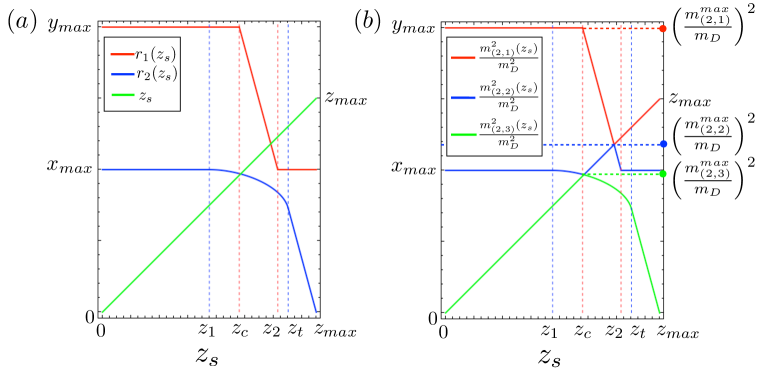
Figure 11: (a) The functional dependence of $r_{1}(z_{s})$ (red line) and $r_{2}(z_{s})$ (blue line), for the case of $x_{0}<y_{0}$ depicted in Fig. 10. (b) The corresponding sorted invariant masses $m_{(2,1)}^{2}(z_{s})$ (red line), $m_{(2,2)}^{2}(z_{s})$ (blue line) and $m_{(2,3)}^{2}(z_{s})$ (green line).

This is depicted more clearly in Fig. 11(a), where we track the functional dependence of $r_{1}(z_{s})$ and $r_{2}(z_{s})$. At first, for very small values of $z_{s}$ (panels (a) and (b) in Fig. 10), both $r_{1}(z_{s})$ and $r_{2}(z_{s})$ stay constant at $r_{1}(z_{s})=y_{0}$ and $r_{2}(z_{s})=x_{0}$. As the value of $z_{s}$ is being increased, the blue point marking the location of $r_{2}$ is lowered until it eventually reaches the diagonal line of $x=y$. This occurs at a special value of $z_{s}\equiv z_{1}$ such that

$$z_{s}=z_{1}\equiv z^{\pm}(x=x_{0},y=x_{0})=z_{0}\left(1-\frac{x_{0}}{y_{0}}\right).$$ (68)

As we continue to increase $z_{s}$ beyond $z_{1}$ and up to $z_{c}$ (panels (c) and (d) in Fig. 10), two effects take place. First, the value of $r_{2}$ is not given by $x_{0}$ any more, but is obtained from the folding along the $x=y$ line. The functional dependence $r_{2}(z_{s})$ is thus given implicitly by the equation

$$z^{+}(r_{2},r_{2})=z_{s}.$$ (69)

Second, the red point in Fig. 10(a-d) indicating the value of $r_{1}$ moves to the left, until it eventually reaches the point $(x,y)=(0,y_{0})$, where the $z$ coordinate is given by

$$z_{s}=z_{c}\equiv z^{\pm}(x=0,y=y_{0})=z_{0}\,e^{-2\eta}.$$ (70)

Comparing to (60), we see that the scan depicted in Fig. 10(d) is taken through point $P_{1}$ in Fig. 9, and from that point on, the value of $r_{1}$ will begin to decrease with $z_{s}$. Indeed, as the value of $z_{s}$ increases further from $z_{c}$ to $z_{2}$ (panels (e) and (f) in Fig. 10), the green region shrinks and $r_{1}(z_{s})$ decreases linearly with $z_{s}$ as

$$r_{1}(z_{s})=\frac{y_{0}}{2}\left(1+\coth\eta\right)\left(1-\frac{z_{s}}{z_{0}}\right),$$ (71)

until $r_{1}(z_{s})$ reaches the value $x_{0}$. This occurs at a value of $z_{s}=z_{2}$ such that $r_{1}(z_{2})=x_{0}$. Inverting (71) and solving for $z_{2}$, we obtain

$$z_{2}=z_{0}\left[1-\frac{x_{0}}{y_{0}}\left(1-e^{-2\,\eta}\right)\right].$$ (72)

Finally, for $z_{s}>z_{2}$, $r_{1}(z_{s})$ again becomes constant at $r_{1}=x_{0}$. Thus the complete functional behavior of $r_{1}(z_{s})$ is given by

$$r_{1}(z_{s})=\left\{\begin{array}[]{l l}y_{0}&\hbox{for }0\leq z_{s}\leq z_{c};\\ \frac{y_{0}}{2}\left(1+\coth\eta\right)\left(1-\frac{z_{s}}{z_{0}}\right)&\hbox{for }z_{c}<z_{s}\leq z_{2};\\ x_{0}&\hbox{for }z_{2}<z_{s}\leq z_{0},\end{array}\right.$$ (76)

as illustrated by the red solid line in Fig. 11(a).

In order to complete the discussion of Figs. 10 and 11, we again turn our focus to $r_{2}(z_{s})$, which was given implicitly by (69). However, this is true only as long as the CT images are crossed by the diagonal line $x=y$. Eventually, as $z_{s}$ approaches its maximal value $z_{0}$, the CT image is confined to the region with $x\sim x_{0}$ and $y\sim 0$ and may not extend all the way up to the $x=y$ line, as depicted in Fig. 10(h). As shown in Fig. 10(g), the image becomes “disconnected” from the diagonal line $x=y$ at the point

$$z_{s}=z_{t}=\frac{z_{0}}{2}\left(1-\frac{x_{0}}{y_{0}}+\sqrt{\left(1-\frac{x_{0}}{y_{0}}\right)^{2}+4\,\frac{x_{0}}{y_{0}}\,e^{-2\,\eta}}\right).$$ (77)

From that point on, for $z_{s}>z_{t}$, the value of $r_{2}$ is determined by the rightmost point of the hatched green CT image, i.e., the blue point in Fig. 10(h). Thus we find that for $z_{s}>z_{t}$, the functional dependence of $r_{2}(z_{s})$ is given by

$$r_{2}(z_{s})=\frac{y_{0}}{2}\left(1+\coth\eta\right)\left(1-\frac{z_{s}}{z_{0}}\right).$$ (78)

Interestingly, this is the same function as (71). This can also be seen by inspecting Fig. 11(a), where the blue and red slanted straight segments are lined up.

In conclusion, we comment on the relative ordering of the special points $\{z_{1},z_{c},z_{2},z_{t}\}$. First, the definition (77) can be rewritten as

$$z_{t}=\frac{1}{2}\left[z_{2}-\frac{x_{0}}{y_{0}}\,z_{c}+\sqrt{\left(z_{2}+\frac{x_{0}}{y_{0}}\,z_{c}\right)^{2}+4\,\frac{x_{0}}{y_{0}}\,z_{c}(z_{0}-z_{2})\,}\right],$$ (79)

which makes it evident that $z_{t}>z_{2}$. Furthermore, the definition (72) can be rewritten as

$$z_{2} = z_{1}+\frac{x_{0}}{y_{0}}\,z_{c}$$ (80a)

$$= z_{c}+\left(1-\frac{x_{0}}{y_{0}}\right)\left(1-e^{-2\eta}\right)\,z_{0}.$$ (80b)

Since $e^{-2\eta}=R_{BC}\leq 1$ by definition and $x_{0}<y_{0}$ by the assumption of this subsection, Eqs. (80) imply that $z_{2}$ is larger than both $z_{1}$ and $z_{c}$. Finally, the relative size of $z_{c}$ and $z_{1}$ is not predetermined, but depends on the mass spectrum. Therefore, the ordering is

$$\left\{z_{1},z_{c}\right\}\leq z_{2}\leq z_{t}.$$ (81)

We are now in position to derive the endpoints of the ranked invariant mass variables. We first add the straight line $z=z_{s}$ as the green line in Fig. 11(a), and proceed to order $\{r_{1}(z_{s}),\,r_{2}(z_{s}),\,z_{s}\}$ for each value of $z_{s}$ as shown in Fig. 11(b), where the red, blue, and green colored curves track the values of the largest, the second largest, and the smallest invariant mass combination for each $z_{s}$. Therefore, the endpoint of each ranked invariant mass arises at the maximum of each colored curve. Since $r_{1}$ and $r_{2}$ have already been ordered among themselves in accordance with (64), all that is left to do now is to compare $r_{1}(z_{s})$ and $r_{2}(z_{s})$ to the value of $z_{s}$ itself. This leads to two interesting intersection points seen in Fig. 11(a): first, the intersection point between $r_{1}(z_{s})$ and the straight line $z_{s}$

$$r_{1}(z_{s})=z_{s}\Longleftrightarrow z_{s}=r_{1z}\equiv\frac{\left(1-R_{CD}\right)\left(1-R_{AB}\right)}{2-R_{AB}},$$ (82)

and the corresponding intersection point between $r_{2}(z_{s})$ and the straight line $z_{s}$

$$r_{2}(z_{s})=z_{s}\Longleftrightarrow z_{s}=r_{2z} \equiv 1-R_{CD}\left\{2+R_{BC}\left(2-R_{AB}\right)\right\}$$ (83)

$$+ 2\sqrt{R_{BC}R_{CD}\left\{R_{CD}\left(3-R_{AB}\right)-1\right\}}.$$

Armed with these results, it is now straightforward to determine the kinematic endpoints of the sorted invariant mass variables on a case-by-case basis. We postpone the presentation of the relevant results until Section 3.3, after we have had the chance to also discuss the case of $x_{0}>y_{0}$, which is the subject of the next subsection.

3.2.2 CT scans for the case of $x_{0}>y_{0}$

We now repeat the analysis of the previous subsection for the case of $x_{0}>y_{0}$. Note that the vertices $P_{2}$ and $P_{3}$ from Fig. 9 have a common $x$ coordinate $x=x_{0}$ (see also Eqs. (61) and (62)). Therefore, for any value of $z_{s}$, we will have the simple relation (contrast this to (76))

$$r_{1}(z_{s})=x_{0}.$$ (84)

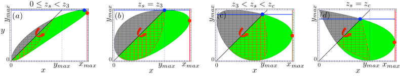
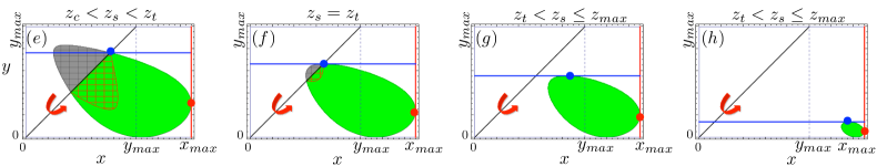
Figure 12: The same as Fig. 10, but for the case of $x_{0}>y_{0}$.

This fact can be clearly observed in Figs. 12 and 13, which are the $x_{0}>y_{0}$ analogues of Figs. 10 and 11, respectively. On the other hand, the behavior of the function $r_{2}(z_{s})$ is similar to the $x_{0}<y_{0}$ case from the previous subsection, only now the roles of $x$ and $y$ are reversed. Again, there are two special points, $z_{s}=z_{3}$ and $z_{s}=z_{t}$, where the functional form of $r_{2}(z_{s})$ changes. Fig. 12(a,b) reveals that as we start increasing $z_{s}$ from 0, the value of $r_{2}$ stays constant at $r_{2}(z_{s})=y_{0}$. Eventually the blue point determining the value of $r_{2}$ reaches the diagonal line $x=y$. This occurs at a special value of $z_{s}=z_{3}$ given by

$$z_{s}=z_{3}=z^{\pm}\left(y_{0},y_{0}\right)=z_{0}\left(1-\frac{y_{0}}{x_{0}}\right)e^{-2\,\eta}.$$ (85)

Once $z_{s}$ exceeds $z_{3}$, the blue point begins to track the straight line of $x=y$ and $r_{2}(z_{s})$ is again found from (69). As illustrated in Fig. 12(c-f), this trend continues until the contour of $z^{+}(x,y)=z_{s}$ is detached from the $x=y$ line at the point $z_{s}=z_{t}$, where $z_{t}$ is again given by (77). Finally, for $z_{s}>z_{t}$, $r_{2}(z_{s})$ is the maximal $y$-coordinate of the contour line $z^{+}(x,y)=z_{s}$ which was already computed earlier in Eq. (71).

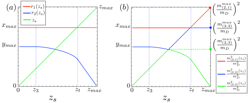
Figure 13: The same as Fig. 11, but for the case $x_{0}>y_{0}$ shown in Fig. 12.

The rest of the steps are identical to those for the previous case of $x_{0}<y_{0}$. Having ranked $x$ and $y$ among themselves in terms of $r_{1}$ and $r_{2}$, it remains to rank $z$ relative to $r_{1}$ and $r_{2}$, as illustrated in Fig. 13(b). The relevant results are summarized in the next subsection.

3.3 Results summary for the $(1,1,1)$ decay topology

In this subsection, we collect all relevant results derived from the arguments in the previous two subsections. We have seen that the endpoints of the ranked invariant mass variables are given in terms of the endpoints $x_{0}$, $y_{0}$ and $z_{0}$ of the original unranked variables (46), as well as the two intersection points (82) and (83). The actual mass spectrum $\{m_{D},m_{C},m_{B},m_{A}\}$ then determines which of these five expressions applies to which ranked variable. Therefore, in presenting the results, we must first describe how the mass parameter space $\{m_{D},m_{C},m_{B},m_{A}\}$ is partitioned into domains, and then specify the relevant endpoint formulas for each individual domain.

In order to define the domains, we can factor out the overall scale, say $m_{D}$, and then trade the remaining three mass variables $\{m_{C},m_{B},m_{A}\}$ for the dimensionless ratios (15). Even though the resulting parameter space $\{R_{AB},R_{BC},R_{CD}\}$ is three-dimensional, it turns out that all relevant domains can be exhibited on a suitably chosen 2-dimensional slice at constant $R_{AB}$, as illustrated in Figs. 14 and 15.

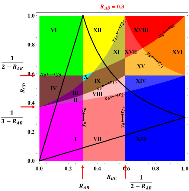
Figure 14: The colors indicate the relevant definition domains for the endpoint formulas (112) in the $(R_{BC},R_{CD})$ plane for fixed $R_{AB}=0.3$. Note the presence of Region $X$ (the cyan triangular-shaped region) at this relatively low value of $R_{AB}$. The solid black curves denote the domains relevant for the $m_{(3,1)}$ endpoint formulas (117).

The color coding in Figs. 14 and 15 shows that there are 18 different regions which are needed in order to define the endpoints of the sorted two-body invariant mass variables $m_{(2,r)}$. Sixteen of those regions are always visible, for any value of the fixed parameter $R_{AB}$. On the other hand, Region $X$ only appears at low values of $R_{AB}$, $R_{AB}<(3-\sqrt{5})/2$ (see Fig. 14), while Region $V$ only appears at high values of $R_{AB}$, $R_{AB}>(3-\sqrt{5})/2$ (see Fig. 15). In what follows, each region will be defined by specifying a range of $R_{BC}$ values and a corresponding range for $R_{CD}$ values. Given the geometry of Figs. 14 and 15, it is convenient to define the region boundaries at a fixed $R_{AB}$ by treating $R_{BC}$ as the independent variable, and $R_{CD}$ as the dependent variable, as follows:

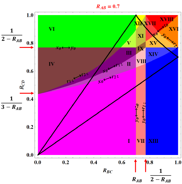
Figure 15: The same as Fig. 14 but for $R_{AB}=0.7$. Note the disappearance of Region $X$ and the emergence of Region $V$ (the yellowgreen triangular-shaped region).

$$x_{0}\leftrightarrow r_{2z}:\quad R_{CD} = f_{x_{0}\leftrightarrow r_{2z}}(R_{BC})\equiv\frac{1}{3-R_{AB}-R_{BC}},$$ (86)

$$x_{0}\leftrightarrow r_{1z}:\quad R_{CD} = f_{x_{0}\leftrightarrow r_{1z}}(R_{BC})\equiv\frac{1}{3-R_{AB}-(2-R_{AB})R_{BC}},$$ (87)

$$r_{1z}\leftrightarrow r_{2z}:\quad R_{CD} = f_{r_{1z}\leftrightarrow r_{2z}}(R_{BC})\equiv\frac{1}{3-R_{AB}-(2-R_{AB})^{2}R_{BC}},$$ (88)

$$x_{0}\leftrightarrow y_{0}:\quad R_{CD} = f_{x_{0}\leftrightarrow y_{0}}(R_{BC})\equiv\frac{1}{2-R_{AB}},$$ (89)

$$x_{0}\leftrightarrow z_{0}:\quad R_{CD} = f_{x_{0}\leftrightarrow z_{0}}(R_{BC})\equiv\frac{1}{2-R_{BC}},$$ (90)

$$y_{0}\leftrightarrow r_{2z}:\quad R_{CD} = f_{y_{0}\leftrightarrow r_{2z}}(R_{BC})\equiv\frac{1}{3-R_{AB}-R^{-1}_{BC}}.$$ (91)

The functions $f(R_{BC})$ defining those boundaries are labelled by the replacement which needs to be done in the endpoint formulas (112) below as one crosses the corresponding boundary and moves from one region to the next.

In addition, Figs. 14 and 15 also display two vertical boundaries

$$y_{0}\leftrightarrow z_{0}:\quad R_{BC} = f_{y_{0}\leftrightarrow z_{0}}(R_{AB})\equiv R_{AB},$$ (92)

$$y_{0}\leftrightarrow r_{1z}:\quad R_{BC} = f_{y_{0}\leftrightarrow r_{1z}}(R_{AB})\equiv\frac{1}{2-R_{AB}}.$$ (93)

Region		$R_{CD}$ range		$R_{BC}$ range
Label	Color	min	max	min	max
$I$	magenta	0	$f_{x_{0}\leftrightarrow r_{2z}}$
$II$	orchid	$f_{x_{0}\leftrightarrow r_{2z}}$	$f_{x_{0}\leftrightarrow r_{1z}}$
$III$	purple	$f_{x_{0}\leftrightarrow r_{1z}}$	$\min(f_{r_{1z}\leftrightarrow r_{2z}},f_{x_{0}\leftrightarrow y_{0}})$	0	$f_{y_{0}\leftrightarrow z_{0}}$
$IV$	brown	$f_{r_{1z}\leftrightarrow r_{2z}}$	$f_{x_{0}\leftrightarrow y_{0}}$
$V$	yellowgreen	$f_{x_{0}\leftrightarrow y_{0}}$	$f_{r_{1z}\leftrightarrow r_{2z}}$
$VI$	green	$\max(f_{x_{0}\leftrightarrow y_{0}},f_{r_{1z}\leftrightarrow r_{2z}})$	1
$VII$	lightsalmon	0	$f_{x_{0}\leftrightarrow r_{2z}}$
$VIII$	pink	$f_{x_{0}\leftrightarrow r_{2z}}$	$f_{x_{0}\leftrightarrow r_{1z}}$
$IX$	brown	$f_{x_{0}\leftrightarrow r_{1z}}$	$\min(f_{x_{0}\leftrightarrow z_{0}},f_{r_{1z}\leftrightarrow r_{2z}})$	$f_{y_{0}\leftrightarrow z_{0}}$	$f_{y_{0}\leftrightarrow r_{1z}}$
$X$	cyan	$f_{r_{1z}\leftrightarrow r_{2z}}$	$f_{x_{0}\leftrightarrow z_{0}}$
$XI$	darkkhaki	$f_{x_{0}\leftrightarrow z_{0}}$	$f_{r_{1z}\leftrightarrow r_{2z}}$
$XII$	yellow	$\max(f_{r_{1z}\leftrightarrow r_{2z}},f_{x_{0}\leftrightarrow z_{0}})$	1
$XIII$	blue	0	$f_{x_{0}\leftrightarrow r_{2z}}$
$XIV$	skyblue	$f_{x_{0}\leftrightarrow r_{2z}}$	$f_{x_{0}\leftrightarrow y_{0}}$
$XV$	coral	$f_{x_{0}\leftrightarrow y_{0}}$	$\min(f_{x_{0}\leftrightarrow z_{0}},f_{y_{0}\leftrightarrow r_{2z}})$	$f_{y_{0}\leftrightarrow r_{1z}}$	1
$XVI$	orange	$f_{y_{0}\leftrightarrow r_{2z}}$	$f_{x_{0}\leftrightarrow z_{0}}$
$XVII$	fuchsia	$f_{x_{0}\leftrightarrow z_{0}}$	$f_{y_{0}\leftrightarrow r_{2z}}$
$XVIII$	red	$\max(f_{x_{0}\leftrightarrow z_{0}},f_{y_{0}\leftrightarrow r_{2z}})$	1

Table 1: Definition of the colored regions seen in Figs. 14 and 15.

Using the definitions of the boundaries (86-93), the 18 colored regions seen in Figs. 14 and 15 can be explicitly defined as in Table 1. Then, the kinematic endpoints for the sorted two-body invariant mass variables $m_{(2,r)}$ are given by

$$(m_{(2,1)}^{\max},m_{(2,2)}^{\max},m_{(2,3)}^{\max}) = m_{D}\times\left\{\begin{array}[]{l l l}\left(\sqrt{y_{0}},\sqrt{r_{1z}},\sqrt{x_{0}}\right)&\text{in Region I}\\ \left(\sqrt{y_{0}},\sqrt{r_{1z}},\sqrt{r_{2z}}\right)&\text{in Region II}\\ \left(\sqrt{y_{0}},\sqrt{x_{0}},\sqrt{r_{2z}}\right)&\text{in Region III}\\ \left(\sqrt{y_{0}},\sqrt{x_{0}},\sqrt{r_{1z}}\right)&\text{in Region IV}\\ \left(\sqrt{x_{0}},\sqrt{y_{0}},\sqrt{r_{2z}}\right)&\text{in Region V}\\ \left(\sqrt{x_{0}},\sqrt{y_{0}},\sqrt{r_{1z}}\right)&\text{in Region VI}\\ \left(\sqrt{z_{0}},\sqrt{r_{1z}},\sqrt{x_{0}}\right)&\text{in Region VII}\\ \left(\sqrt{z_{0}},\sqrt{r_{1z}},\sqrt{r_{2z}}\right)&\text{in Region VIII}\\ \left(\sqrt{z_{0}},\sqrt{x_{0}},\sqrt{r_{2z}}\right)&\text{in Region IX}\\ \left(\sqrt{z_{0}},\sqrt{x_{0}},\sqrt{r_{1z}}\right)&\text{in Region X}\\ \left(\sqrt{x_{0}},\sqrt{z_{0}},\sqrt{r_{2z}}\right)&\text{in Region XI}\\ \left(\sqrt{x_{0}},\sqrt{z_{0}},\sqrt{r_{1z}}\right)&\text{in Region XII}\\ \left(\sqrt{z_{0}},\sqrt{y_{0}},\sqrt{x_{0}}\right)&\text{in Region XIII}\\ \left(\sqrt{z_{0}},\sqrt{y_{0}},\sqrt{r_{2z}}\right)&\text{in Region XIV}\\ \left(\sqrt{z_{0}},\sqrt{x_{0}},\sqrt{r_{2z}}\right)&\text{in Region XV}\\ \left(\sqrt{z_{0}},\sqrt{x_{0}},\sqrt{y_{0}}\right)&\text{in Region XVI}\\ \left(\sqrt{x_{0}},\sqrt{z_{0}},\sqrt{r_{2z}}\right)&\text{in Region XVII}\\ \left(\sqrt{x_{0}},\sqrt{z_{0}},\sqrt{y_{0}}\right)&\text{in Region XVIII}\\ \end{array}\right..$$ (112)

For completeness, we also list the well known endpoint formulas for the three-body invariant mass $m_{(3,1)}$ Allanach:2000kt ; Gjelsten:2004ki

$$m_{(3,1)}^{\max} = m_{D}\times\left\{\begin{array}[]{l l}\sqrt{(1-R_{CD})(1-R_{AB}R_{BC})},&\text{ for }R_{CD}<R_{AB}R_{BC};\\[5.69054pt] \sqrt{(1-R_{BC})(1-R_{CD}R_{AB})},&\text{ for }R_{BC}<R_{AB}R_{CD};\\[5.69054pt] \sqrt{(1-R_{AB})(1-R_{BC}R_{CD})},&\text{ for }R_{AB}<R_{BC}R_{CD};\\[5.69054pt] \sqrt{(1-\sqrt{R_{AB}R_{BC}R_{CD}})},&\text{ otherwise.}\end{array}\right.$$ (117)

4 Type $(2,1)$ cascade decay chain

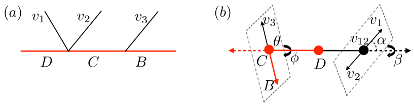
Figure 16: (a) Type $(2,1)$ cascade decay chain. Here $v_{i}$, $(i=1,2,3)$, represents a visible SM particle, while $B$, $C$, and $D$ are new physics particles. (b) The relevant kinematics in the rest frame of particle $D$. Here $\alpha$ is the polar angle of $v_{1}$ with respect to the direction of the composite system of $v_{1}\oplus v_{2}$, $\theta$ is the polar angle of $v_{3}$ with respect to the direction of $D$ in the rest frame of particle $C$, and $\beta$ and $\phi$ are respectively the azimuthal angles of $v_{1}$ and $v_{3}$ about the axis defined by particles $C$ and $D$.

In this section, we proceed to analyze one of the hybrid decay topologies, namely type $(2,1)$. The relevant decay chain is depicted in Fig. 16(a): a massive particle $D$ decays via a three-body decay into two massless visible particles $v_{1}$ and $v_{2}$ and an on-shell intermediate particle $C$. In turn, particle $C$ decays into a massless visible particle $v_{3}$ and an invisible particle $B$. The relevant decay configuration seen in the rest frame of particle $D$ is illustrated in Fig. 16(b). Again, naïvely there exist four degrees of freedom, however, out of the two azimuthal angles, $\beta$ and $\phi$, only their difference is relevant — we can then safely parametrize it with $\phi$, and set $\beta$ to zero.

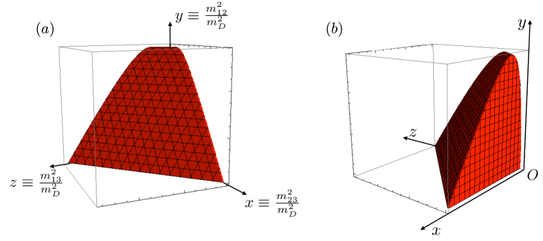
Figure 17: Two different views of the allowed phase space for a $(2,1)$ cascade decay chain, in terms of the dimensionless variables (47-49). The boundary surface is given by Eqs. (119-121). In order to study the ranked invariant mass distributions, here we scan at a fixed $y$ value $y_{s}$. For this illustration, the mass spectrum has been chosen as $\left(m_{D},m_{C},m_{B}\right)=\left(1000,700,500\right)$ GeV.

The allowed $\{x,y,z\}$ phase space is shown in Fig. 17. In order to obtain the equation for the surface boundary of the allowed region, we start from the kinematic relation

$$x+z = 1+R_{BC}R_{CD}-y-\frac{2E_{B}^{(D)}}{m_{D}}$$ (118)

$$= \frac{1-R_{BC}}{2}\left[1-R_{CD}-y-\sqrt{(1+R_{CD}-y)^{2}-4R_{CD}}\cos\theta\right],$$

where the superscript on $E_{B}$ implies that this energy is measured in the rest frame of particle $D$. Notice that the symmetry $v_{1}\leftrightarrow v_{2}$ implies that the variables $x$ and $z$ always enter in the combination $x+z$. Then, the equation for the boundary surface is

$$x+z=\Sigma^{\pm}(y),$$ (119)

where the functions $\Sigma^{\pm}(y)$, which are the analogues of (57,58), are obtained from (118) for the extreme values of $\cos\theta$:

$$\Sigma^{+}_{(x,z)}(y) \equiv \max_{y}(x+z)=\frac{1-R_{BC}}{2}\left[1-R_{CD}-y+\sqrt{\left(1+R_{CD}-y\right)^{2}-4R_{CD}}\right],$$ (120)

$$\Sigma^{-}_{(x,z)}(y) \equiv \min_{y}(x+z)=\frac{1-R_{BC}}{2}\left[1-R_{CD}-y-\sqrt{\left(1+R_{CD}-y\right)^{2}-4R_{CD}}\right].$$ (121)

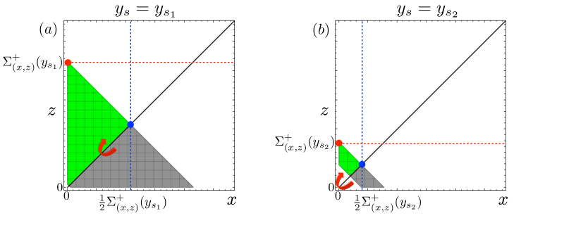
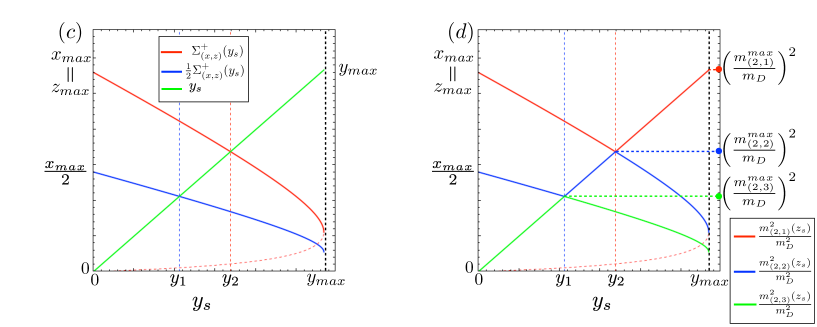
Figure 18: (a,b): CT-images in the $(x,z)$ plane, for a small (left) and a large (right) value of $y_{s}$. Due to the $x\leftrightarrow z$ symmetry, the green and grey halves of the CT image are identical. (c,d) Illustration of the ranking procedure among $x$, $y$ and $z$, in analogy to Figs. 11 and 13.

In order to derive the maximal values of the sorted invariant masses of order 2, we repeat the scanning procedure from the previous section, only now we scan along the $y$-axis. For a given $y=y_{s}$, the CT image in the $(x,z)$ plane is an isosceles trapezoid, as shown in Fig. 18. We again rank $x(y_{s})$ and $z(y_{s})$ for all possible pairs of $(x,z)$ to obtain the ranked variables

$$r_{1}\equiv\max\left\{\max\left[x(y_{s}),\;z(y_{s})\right]\right\},\quad r_{2}\equiv\max\left\{\min\left[x(y_{s}),\;z(y_{s})\right]\right\}.$$ (122)

Due to the simple geometry of Fig. 18(a,b), $r_{1}$ and $r_{2}$ can be readily computed as

$$r_{1}(y_{s}) = \Sigma^{+}_{(x,z)}(y)=\frac{1-R_{BC}}{2}\left[1-R_{CD}-y+\sqrt{\left(1+R_{CD}-y\right)^{2}-4R_{CD}}\right],$$ (123)

$$r_{2}(y_{s}) = \frac{\Sigma^{+}_{(x,z)}(y)}{2}=\frac{1-R_{BC}}{4}\left[1-R_{CD}-y+\sqrt{\left(1+R_{CD}-y\right)^{2}-4R_{CD}}\right].$$ (124)

We then compare the variables $r_{1}(y_{s})$, $r_{2}(y_{s})$, and $y=y_{s}$ as before, see Fig. 18(c,d). There are two special points, denoted by $y_{1}$ and $y_{2}$, which arise from the intersection of $r_{2}(y_{s})$ and $r_{1}(y_{s})$ with the straight line $y=y_{s}$:

$$\frac{1}{2}\Sigma^{+}_{(x,z)}(y_{1})=y_{1}~{}~{} \rightarrow ~{}~{}y_{1}=\frac{1}{2}\left(1-R_{BC}\right)\left[\frac{2}{3-R_{BC}}-R_{CD}\right],$$ (125)

$$\Sigma^{+}_{(x,z)}(y_{2})=y_{2}~{}~{} \rightarrow ~{}~{}y_{2}=\left(1-R_{BC}\right)\left[\frac{1}{2-R_{BC}}-R_{CD}\right].$$ (126)

The kinematic endpoints for the sorted two-body invariant masses $m_{(2,r)}$ will be given in terms of the endpoints $x_{0}=z_{0}$ and $y_{0}$ of the original unsorted variables and the two special points $y_{1}$ and $y_{2}$ given by (125) and (126). Fig. 18(d) shows an example where $m_{(2,1)}^{max}=m_{D}\sqrt{y_{0}}$, $m_{(2,2)}^{max}=m_{D}\sqrt{y_{2}}$ and $m_{(2,3)}^{max}=m_{D}\sqrt{y_{1}}$. The relevant formulas for the general case are collected in Section 4.1.

In conclusion of this subsection, we discuss the derivation of the endpoint of the $m_{(3,1)}$ variable for the case of a type $(2,1)$ decay topology. Since in supersymmetry models one typically gets either $(1,1,1)$ or $(1,2)$ decay topologies, this case has not drawn much attention in the existing literature. It is most convenient to analyze the decay kinematics in the plane of $(x+z)$ versus $y$, as shown in Fig. 19. Since all visible particles are assumed massless, we have the identity

$$\frac{m_{(3,1)}^{2}}{m_{D}^{2}}=x+y+z\equiv k,$$ (127)

which describes a straight line with a slope $-1$ and intercept $k$:

$$x+z=-y+k.$$ (128)

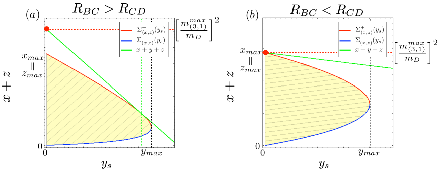
Figure 19: The allowed phase space (yellow-shaded region) of a Type $(2,1)$ decay chain in the $(y,x+z)$ plane. The kinematic boundary is given by $\Sigma^{\pm}_{(x,z)}(y_{s})$ for a given $y_{s}$. The two panels show the two distinct cases for $m_{(3,1)}^{max}$: (a) $R_{BC}>R_{CD}$ and (b) $R_{BC}<R_{CD}$.

Given Eq. (127), in order to maximize $m_{(3,1)}$, we need to maximize the intercept, $k$, with respect to the full allowed phase space of $(y,x+z)$, keeping the slope fixed at $-1$. As shown in Fig. 19, the boundary of the allowed phase space is given by $\Sigma_{(x,z)}^{\pm}(y)$, and we need to consider two distinct cases, illustrated in panels (a) and (b). Note that $\Sigma_{(x,z)}^{+}(y)$ is a monotonically decreasing function of $y$, whose (negative) slope increases in magnitude and approaches $-\infty$ at $y=y_{\max}$. Therefore, if the slope at $y=0$ is larger than $-1$, then Eq. (128) will appear as a tangential line on the curve of $\Sigma_{(x,z)}^{+}(y)$ as shown in Fig. 19(a), and the resulting $k$ will give rise to the maximum $m_{(3,1)}$. If, however, the slope at $y=0$ is already smaller than $-1$, then no such tangential line is possible, and the line giving the maximum will pass through $(y,x+z)=(0,\Sigma^{+}_{(x,z)}(0))$, as shown in Fig. 19(b). A simple algebra results in the following kinematic endpoints:

$$k_{\max}=\left\{\begin{array}[]{ll}(1-\sqrt{R_{BC}R_{CD}})^{2},&R_{CD}<R_{BC};\\[5.69054pt] (1-R_{BC})(1-R_{CD}),&\text{otherwise.}\end{array}\right.$$ (131)

4.1 Results summary for the $(2,1)$ decay topology

The endpoints of the $m_{(2,r)}$ and $m_{(3,1)}$ sorted invariant mass variables are given in terms of the nominal endpoints

$$x_{0} \equiv x_{max}=(1-R_{BC})(1-R_{CD}),$$ (132)

$$y_{0} \equiv y_{max}=(1-\sqrt{R_{CD}})^{2},$$ (133)

and the intersection points $y_{1}$ and $y_{2}$ given by (125) and (126). The endpoint formulas are again piecewise-defined functions, and the boundaries of the defining regions are given by functions $R_{CD}=f(R_{BC})$ in analogy to (86-91):

$$x_{0}\leftrightarrow y_{0}:\quad R_{CD} = f_{x_{0}\leftrightarrow y_{0}}(R_{BC})\equiv\frac{R^{2}_{BC}}{(2-R_{BC})^{2}},$$ (134)

$$y_{2}\leftrightarrow x_{0}/2:\quad R_{CD} = f_{y_{2}\leftrightarrow x_{0}/2}(R_{BC})\equiv\frac{R_{BC}}{(2-R_{BC})},$$ (135)

$$y_{0}\leftrightarrow y_{1}:\quad R_{CD} = f_{y_{0}\leftrightarrow y_{1}}(R_{BC})\equiv\frac{4}{(3-R_{BC})^{2}}.$$ (136)

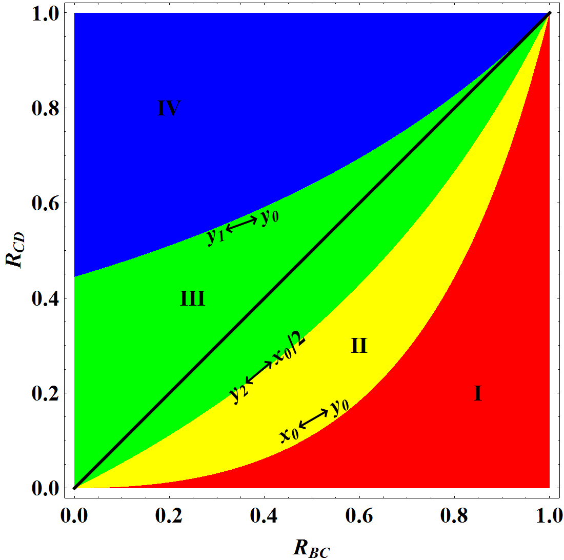
Figure 20: The same as Figs. 14 and 15, but for the Type (2,1) decay topology discussed in Section 4.

The boundaries (134-136) divide the $(R_{BC},R_{CD})$ parameter space of the $(2,1)$ decay topology into the 4 color-coded regions shown in Fig. 20. Then, the kinematic endpoints of the ranked two-body invariant mass distributions are given by

$$(m_{(2,1)}^{\max},m_{(2,2)}^{\max},m_{(2,3)}^{\max}) = m_{D}\times\left\{\begin{array}[]{l l l}\left(\sqrt{y_{0}},\sqrt{y_{2}},\sqrt{y_{1}}\right)&\text{in Region I;}\\[5.69054pt] \left(\sqrt{x_{0}},\sqrt{y_{2}},\sqrt{y_{1}}\right)&\text{in Region II;}\\[5.69054pt] \left(\sqrt{x_{0}},\sqrt{x_{0}/2},\sqrt{y_{1}}\right)&\text{in Region III;}\\[5.69054pt] \left(\sqrt{x_{0}},\sqrt{x_{0}/2},\sqrt{y_{0}}\right)&\text{in Region IV;}\end{array}\right.$$ (141)

while the endpoint of the three-body invariant mass is

$$m_{(3,1)}^{max} = m_{D}\times\left\{\begin{array}[]{l l }1-\sqrt{R_{BC}R_{CD}}&\quad\text{for }R_{CD}<R_{BC};\\[5.69054pt] \sqrt{(1-R_{BC})(1-R_{CD})}&\quad\text{otherwise.}\end{array}\right.$$ (144)

5 Type $(1,2)$ cascade decay chain

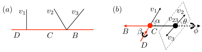
Figure 21: (a) Type $(1,2)$ cascade decay chain. (b) The relevant kinematics in the rest frame of particle $C$. Here $\alpha$ ($\theta$) is the polar angle of $v_{1}$ ($v_{2}$) with respect to the direction of the composite system of $v_{2}\oplus v_{3}$, and $\beta$ and $\phi$ are the azimuthal angles of $v_{1}$ and $v_{2}$ about the axis defined by particles $B$ and $C$.

In this section, we analyze the decay topology of type $(1,2)$, which is depicted in Fig. 21(a). First, a massive particle $D$ decays into a visible particle $v_{1}$ along with an on-shell intermediate particle $C$, and in turn, particle $C$ decays into two visible particles $v_{2}$ and $v_{3}$ and an invisible particle $B$ via a three-body decay. It is convenient to analyze the kinematics in the rest frame of particle $C$, as illustrated in Fig. 21(b). As one might expect, most of the analysis leading to the final formulae will be similar to that of the preceding section.

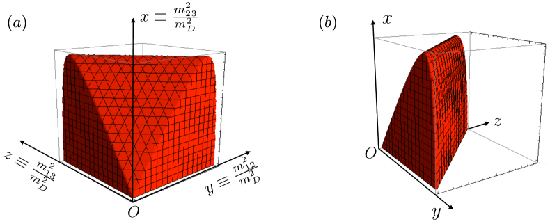
Figure 22: The same as Fig. 22, but for a $(1,2)$ cascade decay chain. The boundary surface is now given by (146-148) and the scanning is done at a fixed value for $x$.

The allowed $\left\{x,y,z\right\}$ phase space is illustrated in Fig. 22. Notice the $y\leftrightarrow z$ symmetry which follows from the $v_{2}\leftrightarrow v_{3}$ symmetry. The boundary of the allowed region can be derived from a kinematic relation analogous to (118):

$$y+z=\frac{1-R_{CD}}{2}\left[1-R_{BC}+\frac{x}{R_{CD}}-\sqrt{\left(1+R_{BC}-\frac{x}{R_{CD}}\right)^{2}-4R_{BC}}\cos\theta\right].$$ (145)

The boundary equation is obtained from here by taking $\cos\theta=\pm 1$. One finds

$$y+z=\Sigma^{\pm}(x),$$ (146)

where

$$\Sigma^{+}_{(y,z)}(x) = \frac{1-R_{CD}}{2}\left[1-R_{BC}+\frac{x}{R_{CD}}+\sqrt{\left(1+R_{BC}-\frac{x}{R_{CD}}\right)^{2}-4R_{BC}}\right],$$ (147)

$$\Sigma^{-}_{(y,z)}(x) = \frac{1-R_{CD}}{2}\left[1-R_{BC}+\frac{x}{R_{CD}}-\sqrt{\left(1+R_{BC}-\frac{x}{R_{CD}}\right)^{2}-4R_{BC}}\right].$$ (148)

In order to find the largest two-body invariant masses, we again scan the allowed phase space shown in Fig. 22, this time at fixed values for $x=x_{s}$. The obtained images are again isosceles trapezoids with bases of length $\Sigma^{+}_{(y,z)}(x_{s})$ and $\Sigma^{-}_{(y,z)}(x_{s})$, as shown in Fig. 23(a,b). We then rank $y(x_{s})$ and $z(x_{s})$ in analogy to (64) and (124)

$$r_{1}\equiv\max\left\{\max\left[y(x_{s}),\;z(x_{s})\right]\right\},\quad r_{2}\equiv\max\left\{\min\left[y(x_{s}),\;z(x_{s})\right]\right\}.$$ (149)

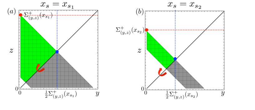
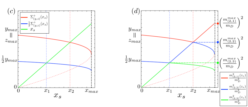
Figure 23: (a,b): CT-images in the $(y,z)$ plane at two fixed values for $x_{s}$, with $x_{s_{1}}<x_{s_{2}}$. Due to the $y\leftrightarrow z$ symmetry, the green and grey halves of the CT image are identical. (c,d) Illustration of the ranking procedure among $x$, $y$ and $z$, in analogy to Figs. 11, 13 and 18(c,d).

Just like the previous case of type $(2,1)$ topology, due to the symmetric structure of the phase space, the corresponding $r_{1}$ and $r_{2}$ are simple to evaluate — they are given by $\Sigma_{(y,z)}^{+}(x_{s})$ and $\Sigma_{(y,z)}^{+}(x_{s})/2$, respectively.

Finally, the ranking procedure among $r_{1}(x_{s})$, $r_{2}(x_{s})$ and $x_{s}$ again introduces two intersection points, $x_{1}$ and $x_{2}$, which arise from the crossing of $r_{2}(x_{s})$ with $x=x_{s}$, and $r_{1}(x_{s})$ with $x=x_{s}$, respectively (see Fig. 23(c,d)):

$$\frac{1}{2}\Sigma^{+}_{(y,z)}(x_{1})=x_{1}~{}~{} \rightarrow ~{}~{}x_{1}=\frac{1-R_{CD}}{2}\left[\frac{1-R_{CD}(3-2R_{BC})}{1-3R_{CD}}\right],$$ (150)

$$\Sigma^{+}_{(y,z)}(x_{2})=x_{2}~{}~{} \rightarrow ~{}~{}x_{2}=\frac{1-R_{CD}}{1-2R_{CD}}\left[1-R_{CD}(2-R_{BC})\right].$$ (151)

The endpoints of the ranked two-body invariant masses $m_{(2,r)}$ will be given in terms of $y_{0}(=z_{0})$, $x_{0}$, $y_{0}/2$, $x_{1}$, or $x_{2}$, depending on the mass spectrum. Fig. 23$(c,d)$ illustrates a specific example where $m_{(2,1)}^{max}=m_{D}\sqrt{x_{0}}$, $m_{(2,2)}^{max}=m_{D}\sqrt{x_{2}}$ and $m_{(2,3)}^{max}=m_{D}\sqrt{x_{1}}$. The relevant formulas for the general case are collected in Section 5.1.

Finally, we discuss the three-body invariant mass $m_{(3,1)}$. The decay topology $(1,2)$ is very common in supersymmetry, e.g., in the decay $\tilde{q}\to q\tilde{\chi}^{0}_{2}$ of a squark $\tilde{q}$ to the second-to-lightest neutralino $\tilde{\chi}^{0}_{2}$, which in turn decays by a three-body decay to the lightest neutralino $\tilde{\chi}^{0}_{1}$ and a couple of jets or leptons: $\tilde{\chi}^{0}_{2}\to q\bar{q}\tilde{\chi}^{0}_{1}$ or $\tilde{\chi}^{0}_{2}\to\ell^{+}\ell^{-}\tilde{\chi}^{0}_{1}$. The expression for the endpoint $m_{(3,1)}^{\max}$ is already known (see, e.g. Lester:2006cf ) and here we shall simply re-derive it using the method from Section 4.

Again, it is convenient to study the variable of interest

$$m_{(3,1)}^{2}=x+y+z\equiv k$$ (152)

in the plane of $(y+z)$ versus $x$, as depicted in Fig. 24, where the allowed region is shaded in yellow. In this plane, the relation (152) again represents a straight line

$$y+z=-x+k.$$ (153)

with constant negative slope $-1$ and intercept $k$. Just like in the previous section, the task is to find the point on the phase space boundary which maximizes the intercept, $k$, for a fixed slope $-1$. As the two panels of Fig. 24 show, one again has to consider two cases, depending on whether the slope of the boundary curve $\Sigma^{+}_{(y,z)}(x)$ at $x=0$ is larger or smaller than $-1$. In the former case, shown in Fig. 24(a), the endpoint $m_{(3,1)}^{\max}$ is obtained from a line tangential to the boundary, while in the latter case the endpoint is simply given by $y_{0}$:

$$m_{(3,1)}^{max} = m_{D}\times\left\{\begin{array}[]{ll}(1-\sqrt{R_{BC}R_{CD}})&R_{CD}>R_{BC},\\[5.69054pt] \sqrt{(1-R_{CD})(1-R_{BC})}&\text{otherwise.}\end{array}\right.$$ (156)

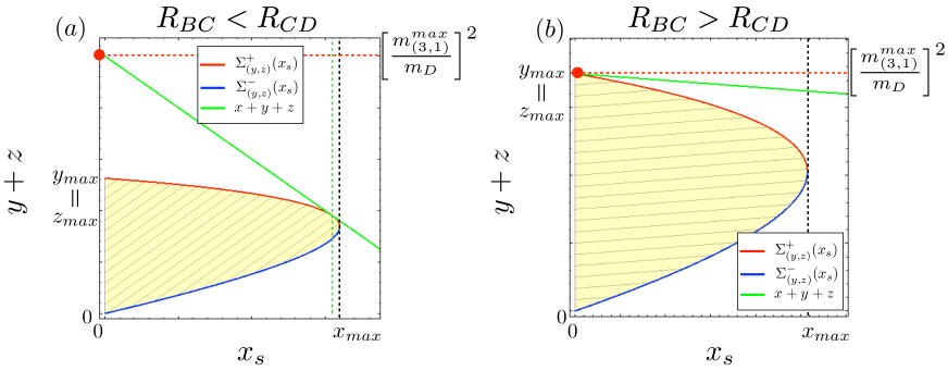
Figure 24: The same as Fig. 19, but for a type $(1,2)$ decay topology, where the relevant phase space is best viewed in the $(x,y+z)$ plane.

5.1 Results summary for the $(1,2)$ decay topology

The endpoints of the $m_{(2,r)}$ and $m_{(3,1)}$ sorted invariant mass variables are given in terms of the nominal endpoints for the $(1,2)$ decay topology

$$x_{0} \equiv x_{max}=R_{CD}\left(1-\sqrt{R_{BC}}\right)^{2},$$ (157)

$$y_{0} \equiv y_{max}=z_{0}\left(\equiv z_{max}\right)=(1-R_{CD})(1-R_{BC}),$$ (158)

and the intersection points $x_{1}$ and $x_{2}$ given by (150) and (151). Again, the formulas are piecewise-defined functions whose relevant domains are illustrated in Fig. 25.

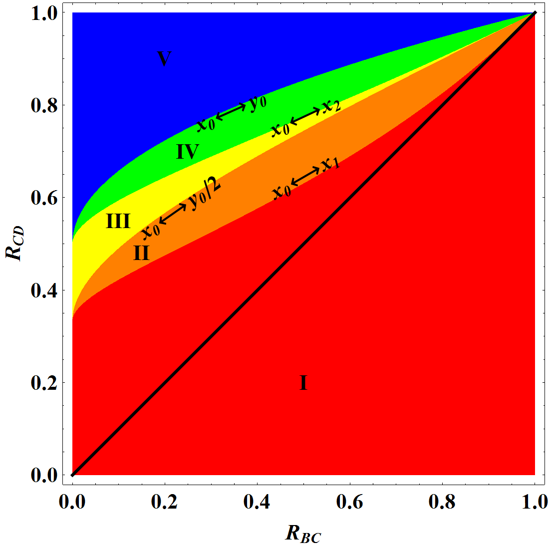
Figure 25: The same as Fig. 20, but for the decay topology of Type $(1,2)$.

In analogy to (134-136) the boundaries of the colored regions in Fig. 25 are defined in terms of the functions $R_{CD}=f(R_{BC})$ as follows:

$$x_{0}\leftrightarrow x_{1}:\quad R_{CD} = f_{x_{0}\leftrightarrow x_{1}}(R_{BC})\equiv\frac{1}{3-2\sqrt{R_{BC}}},$$ (159)

$$x_{0}\leftrightarrow y_{0}/2:\quad R_{CD} = f_{x_{0}\leftrightarrow y_{0}/2}(R_{BC})\equiv\frac{1+\sqrt{R_{BC}}}{3-\sqrt{R_{BC}}},$$ (160)

$$x_{0}\leftrightarrow x_{2}:\quad R_{CD} = f_{x_{0}\leftrightarrow x_{2}}(R_{BC})\equiv\frac{1}{2-\sqrt{R_{BC}}},$$ (161)

$$x_{0}\leftrightarrow y_{0}:\quad R_{CD} = f_{x_{0}\leftrightarrow y_{0}}(R_{BC})\equiv\frac{1+\sqrt{R_{BC}}}{2}.$$ (162)

Unlike the case of the type $(2,1)$ decay topology discussed in Fig. 20, in Fig. 25 we now get 5 different regions.

The kinematic endpoints of the sorted two-body invariant mass distributions are given by

$$(m_{(2,1)}^{\max},m_{(2,2)}^{\max},m_{(2,3)}^{\max}) = m_{D}\times\left\{\begin{array}[]{l l l}\left(\sqrt{y_{0}},\sqrt{y_{0}/2},\sqrt{x_{0}}\right)&\text{in Region I;}\\[5.69054pt] \left(\sqrt{y_{0}},\sqrt{y_{0}/2},\sqrt{x_{1}}\right)&\text{in Region II;}\\[5.69054pt] \left(\sqrt{y_{0}},\sqrt{x_{0}},\sqrt{x_{1}}\right)&\text{in Region III;}\\[5.69054pt] \left(\sqrt{y_{0}},\sqrt{x_{2}},\sqrt{x_{1}}\right)&\text{in Region IV;}\\[5.69054pt] \left(\sqrt{x_{0}},\sqrt{x_{2}},\sqrt{x_{1}}\right)&\text{in Region V;}\end{array}\right.$$ (168)

while the endpoint of the three-body invariant mass is

$$m_{(3,1)}^{max} = m_{D}\times\left\{\begin{array}[]{l l }1-\sqrt{R_{BC}R_{CD}}&\quad\text{for }R_{CD}>R_{BC};\\[5.69054pt] \sqrt{(1-R_{CD})(1-R_{BC})}&\quad\text{otherwise.}\end{array}\right.$$ (171)

6 Conclusions and outlook

The dark matter problem greatly motivates the search for semi-invisibly decaying resonances in Run II of the LHC. After the discovery of such particles, their masses will most likely have to be measured using the classic kinematic endpoint techniques. In fact, such techniques can already be usefully applied in the current data — for example, following the procedure outlined in Burns:2008va , the CMS collaboration has published an analysis of simultaneous extraction of the top, $W$ and neutrino masses from the measurement of kinematic endpoints in the $t\bar{t}$ dilepton system Chatrchyan:2013boa .

In this paper, we revisited the classic method for mass determination via kinematic endpoints, where one studies the invariant mass distributions of suitable collections of visible decay products, and extracts their upper kinematic endpoints. We generalized the existing studies on the subject in several ways:

• We shied away from making any assumptions about the structure of the decay topology, and considered the invariant masses of all possible sets of visible decay products. This led us to the introduction in Eq. (11) of the sorted invariant mass variables $m_{(n,r)}$, where we consider all possible partitions of $n$ visible particles, and then rank the resulting invariant masses in order. The so defined sorted invariant mass variables allow us to study SUSY-like decay chains in a fully model-independent way.

• In Section 2 we considered a completely general semi-invisible decay with no intermediate resonances, where a heavy particle $D$ decays directly to an arbitrary number $N$ of massless SM particles and a single massive NP particle $A$. For this very general case, we derived the corresponding formulas for the endpoints of the sorted invariant mass variables, Eq. (42). The importance of those results lies in the fact that they allow the experimenter to test for the presence of intermediate on-shell resonances between particles $D$ and $A$ — in the absence of such resonances, the ratios of all endpoints are uniquely predicted by Eq. (42). Any measured deviation from those ratios will signal the presence of some other new intermediate particles.

• In the second half of the paper, i.e. Sections 3, 4 and 5, we considered the SUSY-motivated case of $N=3$, and focused on the three possible event topologies with one or two intermediate on-shell particles. Once again, we derived the corresponding formulas for the kinematic endpoints of the sorted invariant mass variables in terms of the physical mass spectrum. Each possible event topology predicts certain correlations among the observed endpoints, as illustrated in Fig. 26.

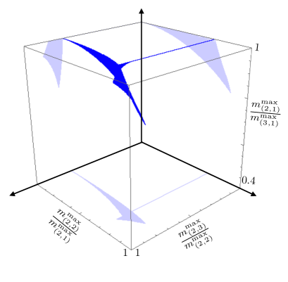
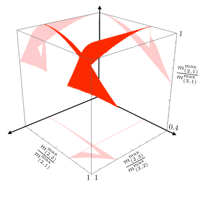
Figure 26: The correlations among the endpoint ratios $x=\frac{m^{max}_{(2,3)}}{m^{max}_{(2,2)}}$, $y=\frac{m^{max}_{(2,2)}}{m^{max}_{(2,1)}}$ and $z=\frac{m^{max}_{(2,1)}}{m^{max}_{(3,1)}}$, for the case of the type $(2,1)$ event topology from Fig. 16(a) (left panel) and the type $(1,2)$ event topology from Fig. 21(a) (right panel). Here the lighter shaded images on each of the three planes $(x,\,y,\,0.4)$, $(0,\,y,\,z)$ and $(x,\,0,\,z)$ are the corresponding projections of the $3D$ surface $(x,y,z)=\left(x(R_{BC},R_{CD}),y(R_{BC},R_{CD}),z(R_{BC},R_{CD})\right)$ which was obtained by scanning over the allowed values of $R_{BC}\in(0,1)$ and $R_{CD}\in(0,1)$. Note that the range of the $z\,$axis is from 0.4 to 1.

In conclusion, we are hoping that the model-independent approach to the kinematic endpoint method presented in this paper will soon be tested in real data after a new physics discovery. At the same time, the results presented here may provide useful mathematical insights to researches interested in phase space kinematics.

- (1) S. Chatrchyan et al. [CMS Collaboration], “Study of the Mass and Spin-Parity of the Higgs Boson Candidate Via Its Decays to Z Boson Pairs,” Phys. Rev. Lett. 110, 081803 (2013) [arXiv:1212.6639 [hep-ex]].
- (2) G. Aad et al. [ATLAS Collaboration], “Evidence for the spin-0 nature of the Higgs boson using ATLAS data,” Phys. Lett. B 726, 120 (2013) [arXiv:1307.1432 [hep-ex]].
- (3) S. Chatrchyan et al. [CMS Collaboration], “Measurement of the properties of a Higgs boson in the four-lepton final state,” Phys. Rev. D 89, 092007 (2014) [arXiv:1312.5353 [hep-ex]].
- (4) S. Arrenberg, H. Baer, V. Barger, L. Baudis, D. Bauer, J. Buckley, M. Cahill-Rowley and R. Cotta et al., “Working Group Report: Dark Matter Complementarity,” arXiv:1310.8621 [hep-ph].
- (5) A. Bartl, H. Fraas and W. Majerotto, “Production and Decay of Neutralinos in e+ e- Annihilation,” Nucl. Phys. B 278, 1 (1986).
- (6) A. Birkedal, K. Matchev and M. Perelstein, “Dark matter at colliders: A Model independent approach,” Phys. Rev. D 70, 077701 (2004) [hep-ph/0403004].
- (7) J. L. Feng, S. Su and F. Takayama, “Lower limit on dark matter production at the large hadron collider,” Phys. Rev. Lett. 96, 151802 (2006) [hep-ph/0503117].
- (8) T. Appelquist, H. C. Cheng and B. A. Dobrescu, “Bounds on universal extra dimensions,” Phys. Rev. D 64, 035002 (2001) [hep-ph/0012100].
- (9) H. C. Cheng, K. T. Matchev and M. Schmaltz, “Bosonic supersymmetry? Getting fooled at the CERN LHC,” Phys. Rev. D 66, 056006 (2002) [hep-ph/0205314].
- (10) A. J. Barr and C. G. Lester, “A Review of the Mass Measurement Techniques proposed for the Large Hadron Collider,” J. Phys. G 37, 123001 (2010) [arXiv:1004.2732 [hep-ph]].
- (11) L. T. Wang and I. Yavin, “A Review of Spin Determination at the LHC,” Int. J. Mod. Phys. A 23, 4647 (2008) [arXiv:0802.2726 [hep-ph]].
- (12) B. C. Allanach, C. G. Lester, M. A. Parker and B. R. Webber, “Measuring sparticle masses in nonuniversal string inspired models at the LHC,” JHEP 0009, 004 (2000) [hep-ph/0007009].
- (13) B. K. Gjelsten, D. J. Miller and P. Osland, “Measurement of SUSY masses via cascade decays for SPS 1a,” JHEP 0412, 003 (2004) [hep-ph/0410303].
- (14) M. Burns, K. T. Matchev and M. Park, “Using kinematic boundary lines for particle mass measurements and disambiguation in SUSY-like events with missing energy,” JHEP 0905, 094 (2009) [arXiv:0903.4371 [hep-ph]].
- (15) F. Moortgat and L. Pape, CMS Physics TDR, Vol. II, Report No. CERN-LHCC-2006, Chap. 13.4, p. 410.
- (16) S. Matsumoto, M. M. Nojiri and D. Nomura, “Hunting for the Top Partner in the Littlest Higgs Model with T-parity at the CERN LHC,” Phys. Rev. D 75, 055006 (2007) [hep-ph/0612249].
- (17) A. Rajaraman and F. Yu, “A New Method for Resolving Combinatorial Ambiguities at Hadron Colliders,” Phys. Lett. B 700, 126 (2011) [arXiv:1009.2751 [hep-ph]].
- (18) Y. Bai and H. C. Cheng, “Identifying Dark Matter Event Topologies at the LHC,” JHEP 1106, 021 (2011) [arXiv:1012.1863 [hep-ph]].
- (19) P. Baringer, K. Kong, M. McCaskey and D. Noonan, “Revisiting Combinatorial Ambiguities at Hadron Colliders with ,” JHEP 1110, 101 (2011) [arXiv:1109.1563 [hep-ph]].
- (20) K. Choi, D. Guadagnoli and C. B. Park, “Reducing combinatorial uncertainties: A new technique based on MT2 variables,” JHEP 1111, 117 (2011) [arXiv:1109.2201 [hep-ph]].
- (21) J. H. Shim and H. S. Lee, “Improving Combinatorial Ambiguities of ttbar Events Using Neural Networks,” Phys. Rev. D 89, 114023 (2014) [arXiv:1402.3907 [hep-ph]].
- (22) H. Baer, D. D. Karatas and X. Tata, “Gluino and Squark Production in Association With Gauginos at Hadron Supercolliders,” Phys. Rev. D 42, 2259 (1990).
- (23) P. Agrawal, C. Kilic, C. White and J. H. Yu, “Improved mass measurement using the boundary of many-body phase space,” Phys. Rev. D 89, 015021 (2014) [arXiv:1308.6560 [hep-ph]].
- (24) K. T. Matchev, F. Moortgat, L. Pape and M. Park, “Precise reconstruction of sparticle masses without ambiguities,” JHEP 0908, 104 (2009) [arXiv:0906.2417 [hep-ph]].
- (25) W. S. Cho, D. Kim, K. T. Matchev and M. Park, “Probing Resonance Decays to Two Visible and Multiple Invisible Particles,” Phys. Rev. Lett. 112, no. 21, 211801 (2014) [arXiv:1206.1546 [hep-ph]].
- (26) E. Byckling and K. Kajantie, “Particle Kinematics”, Wiley, John & Sons, 1973.
- (27) G. F. Giudice, B. Gripaios and R. Mahbubani, “Counting dark matter particles in LHC events,” Phys. Rev. D 85, 075019 (2012) [arXiv:1108.1800 [hep-ph]].
- (28) C. G. Lester, “Constrained invariant mass distributions in cascade decays: The Shape of the ’m(qll)-threshold’ and similar distributions,” Phys. Lett. B 655, 39 (2007) [hep-ph/0603171].
- (29) D. Costanzo and D. R. Tovey, “Supersymmetric particle mass measurement with invariant mass correlations,” JHEP 0904, 084 (2009) [arXiv:0902.2331 [hep-ph]].
- (30) C. Lester, “Mass and Spin Measurement Techniques (for the LHC)”, in “The Dark Secrets of the Terascale : Proceedings, TASI 2011, Boulder, Colorado, USA, Jun 6 - Jul 11, 2011,” Eds. T. Tait and K. Matchev.
- (31) C. G. Lester, M. A. Parker and M. J. White, “Three body kinematic endpoints in SUSY models with non-universal Higgs masses,” JHEP 0710, 051 (2007) [hep-ph/0609298].
- (32) M. Burns, K. Kong, K. T. Matchev and M. Park, “Using Subsystem MT2 for Complete Mass Determinations in Decay Chains with Missing Energy at Hadron Colliders,” JHEP 0903, 143 (2009) doi:10.1088/1126-6708/2009/03/143 [arXiv:0810.5576 [hep-ph]].
- (33) S. Chatrchyan et al. [CMS Collaboration], “Measurement of masses in the system by kinematic endpoints in pp collisions at = 7 TeV,” Eur. Phys. J. C 73, 2494 (2013) doi:10.1140/epjc/s10052-013-2494-7 [arXiv:1304.5783 [hep-ex]].