Milnor Fibre Homology via Deformation

Abstract.

In case of one-dimensional singular locus, we use deformations in order to get refined information about the Betti numbers of the Milnor fibre.

1. Introduction and results

We study the topology of Milnor fibres $F$ of function germs on ${\mathbb{C}}^{n+1}$ with a 1-dimensional singular set. Well known is that $F$ is a $(n-2)$ connected $n$-dimensional CW-complex. What can be said about $H_{n-1}(F)$ and $H_{n}(F)$? In this paper we use deformations in order to get information about these groups. It turns out that the constraints on $F$ yield only small numbers $b_{n-1}(F)$, for which we give upper bounds which are in general sharper than the known ones from [Si4]. The upper Betti number $b_{n}(F)$ can be determined from an Euler characteristic formula. We pay special attention to classes of singularities where $H_{n-1}(F)=0$, where the homology is concentrated in the middle dimension.

The admissible deformations of the function have a singular locus $\Sigma$ consisting of a finite set $R$ of isolated points and finitely many curve branches. Each branch $\Sigma_{i}$ of $\Sigma$ has a generic transversal type (of transversal Milnor fibre $F^{\pitchfork}_{i}$ and Milnor number denoted by $\mu^{\pitchfork}_{i}$) and also contains a finite set $Q_{i}$ of points with non-generic transversal type, which we call special points. In the neighbourhood of each such special point $q$ with Milnor fibre denoted by ${\cal A}_{q}$, there are two monodromies which act on $F^{\pitchfork}_{i}$: the Milnor monodromy of the local Milnor fibration of $F^{\pitchfork}_{i}$, and the vertical monodromy of the local system defined on the germ of $\Sigma_{i}\setminus\{q\}$ at $q$.

In our topological study we work with homology over ${\mathbb{Z}}$ (and therefore we systematically omit ${\mathbb{Z}}$ from the notation of the homology groups). We provide a detailed expression for $H_{n-1}(F)$ through a topological model of $F$ from which we derive the following results.

• If for every component $\Sigma_{i}$ there exist one vertical monodromy $A_{s}$, which has no eigenvalues $1$, then $b_{n-1}(F)=0$. More generally: $b_{n-1}(F)$ is bounded by the sum (taken over the components) of the minimum (over that component) of $\dim\mathop{{\mathrm{ker}}}\nolimits(A_{s}-I)$ (Theorem 4.4).

• Assume that for each irreducible component $\Sigma_{i}$ there is a special singularity at $q$ such that $H_{n-1}({\cal A}_{q})=0$. Then $H_{n-1}(F)=0$.
  More generally: Let $Q^{\prime}:=\{q_{1},\ldots,q_{m}\}\subset Q$ be a subset of special points such that each branch $\Sigma_{i}$ contains at least one of its points. Then (Theorem 4.6b):

  $$b_{n-1}(F)\leq\dim H_{n-1}({\cal A}_{q_{1}})+\cdots+\dim H_{n-1}({\cal A}_{q_{m}}).$$

Note that in both cases already some (small) subset of the special points may have a strong effect and that we may choose the best bound.

In [ST2] we have studied the vanishing homology of projective hypersurfaces with a 1-dimensional singular set. The same type of methods work in the local case. We keep the notations close to those in [ST2] and refer to it for the proof of certain results. In the proof of the main theorems we use the Mayer-Vietoris theorem to study local and (semi) global contributions separately. We construct a CW-complex model of two bundles of transversal Milnor fibres (in §3.4 and §3.5) and their inclusion map (§4). Moreover we use the full strength of the results on local 1-dimensional singularities [Si1], [Si3], [Si4], [Si5], cf also [NS], [Ra], [Ti], [Yo].

We discuss known results such as De Jong’s [dJ] and compute several examples in §5.

Acknowledgment. Most of the research of this paper took place during a Research in Pairs of the authors at the Mathematisches Forschungsinstitut Oberwolfach in November 2015. The authors thank the institute for the support and excellent atmosphere.

2. Local theory of 1-dimensional singular locus

We work with local data of function germs with 1-dimensional singular locus and we will apply results from the well-known theory which we extract from [Si4], [Si5], and [ST2].

Let $f:({\mathbb{C}}^{n+1},0)\to({\mathbb{C}},0)$ be a holomorphic function germ with singular locus $\Sigma$ of dimension 1 and let $\Sigma=\Sigma_{1}\cup\ldots\cup\Sigma_{m}$ be its decomposition into irreducible curve components. Let $E:=B_{\varepsilon}\cap f^{-1}(D_{\delta})$ be the Milnor neighbourhood and $F$ be the local Milnor fibre of $f$, for small enough $\varepsilon$ and $\delta$. The homology $\tilde{H}_{*}(F)$ is concentrated in dimensions $n-1$ and $n$. The non-trivial groups are $H_{n}(F)={\mathbb{Z}}^{\mu_{n}}$, which is free, and $H_{n-1}(F)$ which can have torsion.

There is a well-defined local system on $\Sigma_{i}\setminus\{0\}$ having as fibre the homology of the transversal Milnor fibre $\tilde{H}_{n-1}(F^{\pitchfork}_{i})$, where $F^{\pitchfork}_{i}$ is the Milnor fibre of the restriction of $f$ to a transversal hyperplane section at some $x\in\Sigma_{i}\setminus\{0\}$. This restriction has an isolated singularity whose equisingularity class is independent of the point $x$ and of the transversal section, in particular $\tilde{H}_{*}(F^{\pitchfork}_{i})$ is concentrated in dimension $n-1$. It is on this group that acts the local system monodromy (also called vertical monodromy):

$$A_{i}:\tilde{H}_{n-1}(F^{\pitchfork}_{i})\rightarrow\tilde{H}_{n-1}(F^{\pitchfork}_{i}).$$

After [Si4], one considers a tubular neighbourhood ${\cal N}:=\sqcup_{i=}^{m}{\cal N}_{i}$ of the link of $\Sigma$ and decomposes the boundary $\partial F:=F\cap\partial B_{\varepsilon}$ of the Milnor fibre as $\partial F=\partial_{1}F\cup\partial_{2}F$, where $\partial_{2}F:=\partial F\cap{\cal N}$. Then $\partial_{2}F=\displaystyle{\mathop{\sqcup}^{m}_{i=1}}\partial_{2}F_{i}$, where $\partial_{2}F_{i}:=\partial_{2}F\cap{\cal N}_{i}$.

Each boundary component $\partial_{2}F_{i}$ is fibred over the link of $\Sigma_{i}$ with fibre $F^{\pitchfork}_{i}$. Let then $E^{\pitchfork}_{i}$ denote the transversal Milnor neighbourhood containing the transversal fibre $F^{\pitchfork}_{i}$ and let $\partial_{2}E_{i}$ denote the total space of its fibration above the link of $\Sigma_{i}$. Therefore $E^{\pitchfork}_{i}$ is contractible and $\partial_{2}E_{i}$ retracts to the link of $\Sigma_{i}$. The pair $(\partial_{2}E_{i},\partial_{2}F_{i})$ is related to $A_{i}-I$ via the following exact relative Wang sequence [ST2] ( $n\geq 2$):

(2.1) $$0\rightarrow H_{n+1}(\partial_{2}E_{i},\partial_{2}F_{i})\rightarrow H_{n}(E^{\pitchfork}_{i},F^{\pitchfork}_{i})\stackrel{{\scriptstyle A_{i}-I}}{{\rightarrow}}H_{n}(E^{\pitchfork}_{i},F^{\pitchfork}_{i})\rightarrow H_{n-1}(\partial_{2}E_{i},\partial_{2}F_{i})\rightarrow 0.$$

3. Deformation and vanishing homology

Consider now a 1-parameter family $f_{s}:({\mathbb{C}}^{n+1},0)\to({\mathbb{C}},0)$ where $f_{0}=\hat{f}:({\mathbb{C}}^{n+1},0)\to({\mathbb{C}},0)$ is a given germ with singular locus $\hat{\Sigma}$ of dimension 1, with Milnor data $(\hat{E},\hat{F})$ and $\hat{\Sigma}=\hat{\Sigma_{1}}\cup\ldots\cup\hat{\Sigma_{m}}$ and all the other objects defined like in §2. We use the notation with “hat” since we reserve the notation without “hat” for the deformation $f_{s}$.

We fix a ball $B:=B_{\varepsilon}\subset{\mathbb{C}}^{n+1}$ centered at $0$ and a disk $\Delta:=\Delta_{\delta}\subset{\mathbb{C}}$ at $0$ such that, for small enough radii $\varepsilon$ and $\delta$ the restriction to the punctured disc $\hat{f}_{|}:B\cap f^{-1}(\Delta^{*})\to\Delta^{*}$ is the Milnor fibration of $\hat{f}$.

We say that the deformation $f_{s}$ is admissible if it has good behavior at the boundary, i.e., if for small enough $s$ the family ${f_{s}}_{|}:\partial B\cap f^{-1}(\Delta)\to\Delta$ is stratified topologically trivial.

We choose a value of $s$ which satisfies the above conditions and write from now on $f:=f_{s}$. It then follows that the pair $(E,F):=(B\cap f^{-1}(\Delta),f^{-1}(b))$, where $b\in\partial\Delta$, is topologically equivalent to the Milnor data $(\hat{E},\hat{F})$ of $\hat{f}$. Note that for $f$ we consider the semi-local singular fibration inside $B$ and not just its Milnor fibration at the origin.

Let $\Sigma\subset B$ be the 1-dimensional singular part of the singular set ${\mathrm{Sing\hskip 2.0pt}}(f)\subset B$. Note that $\hat{\Sigma}=\bigcup_{i\in\hat{I}}\hat{\Sigma}$ and $\Sigma=\bigcup_{i\in I}\Sigma_{i}$ can have a different number of irreducible components. It follows that the circle boundaries $\partial B\cap\hat{\Sigma}$ of $\hat{\Sigma}$ identify to the circle boundaries $\partial B\cap\Sigma$ of $\Sigma$ and that the corresponding vertical monodromies are the same.

3.1. Notations

We use notations similar to [ST2] (cf also figure 1).
A point $q$ on $\Sigma$ is called special if the transversal Milnor fibration is not a local product in a neighbourhood of that point.

$Q_{i}:=$ the set of special points on $\Sigma_{i}$; $Q:=\cup_{i\in I}Q_{i}$,
$R:=$ the set of isolated singular points; $R=R_{0}\cup R_{1}$, where $R_{0}$ are the critical points on $f^{-1}(0)$ and $R_{1}$ the critical points outside $f^{-1}(0)$,

$B_{q},B_{r}$ = small enough disjoint Milnor balls within $E$ at the points $q\in Q,r\in R$ resp.
$B_{Q}:=\sqcup_{q}B_{q}$ and $B_{R}:=\sqcup_{r}B_{r}$, and similar notation for $B_{R_{0}}$ and $B_{R_{1}}$,

$\Sigma^{*}_{i}:=\Sigma_{i}\setminus B_{Q}$; $\Sigma^{*}=\cup_{i\in I}\Sigma_{i}^{*}$,
${\cal U}_{i}:=$ small enough tubular neighbourhood of $\Sigma^{*}_{i}$; ${\cal U}=\cup_{i}{\cal U}_{i}$,
$\pi_{\Sigma}:{\cal U}\to\Sigma^{*}$ is the projection of the tubular neighbourhood.
$T=\{f(r)|r\in R\}\cup\{f(\Sigma)\}$ is the set of critical values of $f$ and we assume without loss of generality that $f(\Sigma)=0$.

Let$\{\Delta_{t}\}_{t\in T}$ be a system of non-intersecting small discs $\Delta_{t}$ around each $t\in T$. For any $t\in T$, choose $t^{\prime}\in\partial\Delta_{t}$. If $t=f(r)$ then we denote by $t^{\prime}(r)$ the point $t^{\prime}\in\Delta_{f(r)}$. For $t=0$ we use the notations $t_{0}$ and $t^{\prime}_{0}$ respectively.

Let $E_{r}=B_{r}\cap f^{-1}(\Delta_{f(r)})$ and $F_{r}=B_{r}\cap f^{-1}(t^{\prime}(r))$ be the Milnor data of the isolated singularity of $f$ at $r\in R$. We use next the additivity of vanishing homology with respect to the different critical values and the connected components of ${\mathrm{Sing\hskip 2.0pt}}f$.

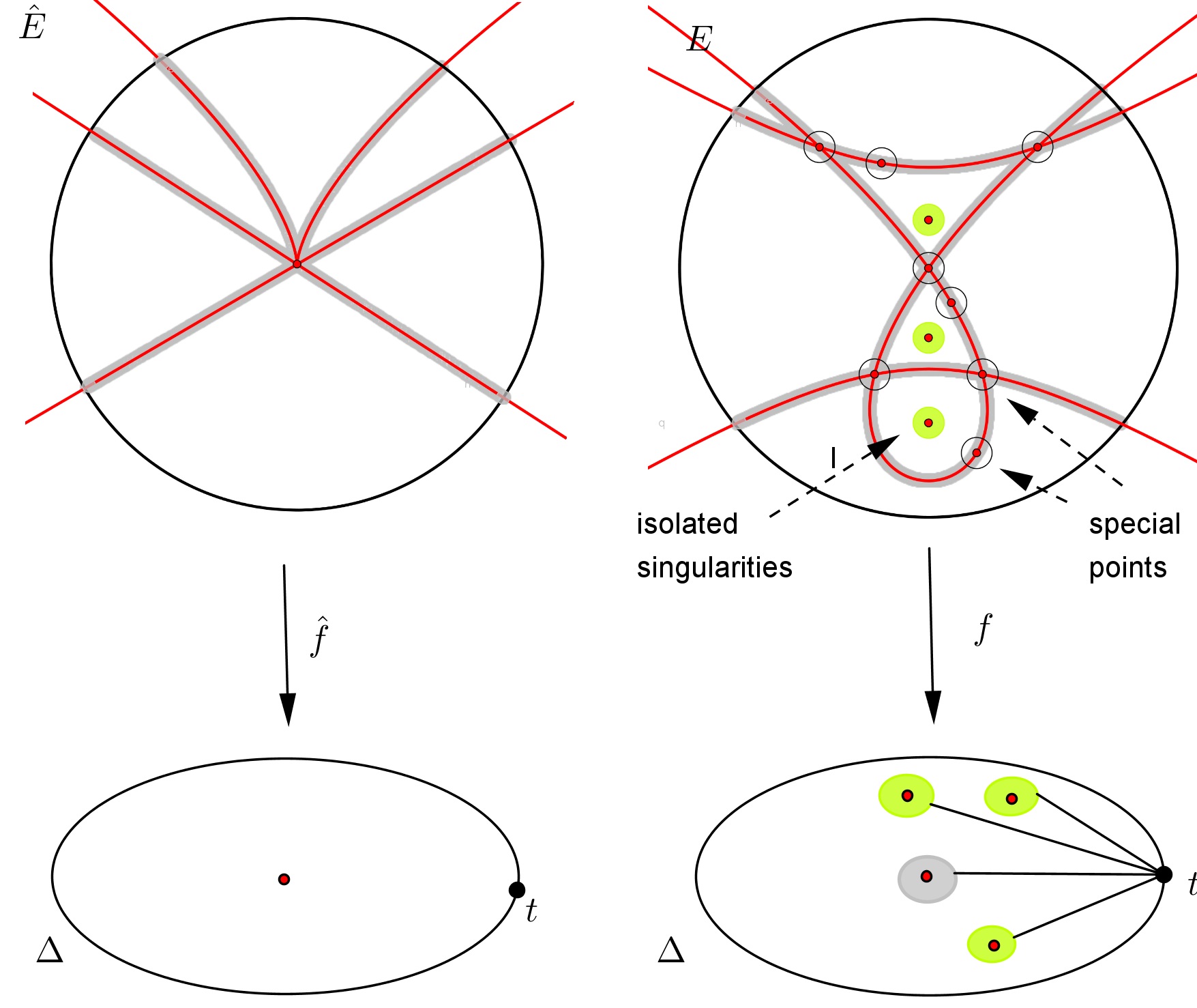
Figure 1. Admissible deformation

By homotopy retraction and by excision we have:

(3.1) $$H_{*}(E,F)\simeq\oplus_{t\in T}H_{*}((f^{-1}(\Delta_{t}),f^{-1}(t^{\prime}))=$$

(3.2) $$=\oplus_{r\in R_{0}}H_{*}(E_{r},F_{r})\oplus H_{*}(E_{0},F_{0})\oplus\oplus_{r\in R_{1}}H_{*}(E_{r},F_{r}),$$

where $(E_{0},F_{0})=(f^{-1}(\Delta_{0})\cap({\cal U}\cup B_{Q}),f^{-1}(t^{\prime}_{0})\cap({\cal U}\cup B_{Q})$ We introduce the following shorter notations:

$$({\cal X}_{q},{\cal A}_{q}):=(f^{-1}(\Delta_{0})\cap B_{q},f^{-1}({t^{\prime}_{0}})\cap B_{q})\;$$

$$\;{\cal X}=\sqcup_{Q}{\cal X}_{q}\;\;,\;\;{\cal A}=\sqcup_{Q}{\cal A}_{q}$$

$${\cal Y}={\cal U}\cap f^{-1}(\Delta_{0})\;,\;{\cal B}:=f^{-1}({t^{\prime}_{0}})\cap{\cal Y}\;\;$$

$${\cal Z}:={\cal X}\cap{\cal Y}\;\;,\;{\cal C}:={\cal A}\cap{\cal B}$$

In these new notations we have:

(3.3) $$H_{*}(E,F)\simeq H_{*}({\cal X}\cup{\cal Y},{\cal A}\cup{\cal B})\oplus\oplus_{r\in R}H_{*}(E_{r},F_{r}).$$

Note that each direct summand $H_{*}(E_{r},F_{r})$ is concentrated in dimension $n+1$ since it identifies to the Milnor lattice ${\mathbb{Z}}^{\mu_{r}}$ of the isolated singularities germs of $f-f(r)$ at $r$, where $\mu_{r}$ denotes its Milnor number. We deal from now on with the term $H_{*}({\cal X}\cup{\cal Y},{\cal A}\cup{\cal B})$ in the direct sum of (3.3).
We consider the relative Mayer-Vietoris long exact sequence:

(3.4) $$\cdots\to H_{*}({\cal Z},{\cal C})\to H_{*}({\cal X},{\cal A})\oplus H_{*}({\cal Y},{\cal B})\to H_{*}({\cal X}\cup{\cal Y},{\cal A}\cup{\cal B})\stackrel{{\scriptstyle\partial_{s}}}{{\to}}\cdots$$

of the pair $({\cal X}\cup{\cal Y},{\cal A}\cup{\cal B})$ and we compute each term of it in the following. The description follows closely [ST2] where we have treated deformations of projective hypersurfaces.

3.2. The homology of $({\cal X},{\cal A})$

One has the direct sum decomposition $H_{*}({\cal X},{\cal A})\simeq\oplus_{q\in Q}H_{*}({\cal X}_{q},{\cal A}_{q})$ since ${\cal X}$ is a disjoint union. The pairs $({\cal X}_{q},{\cal A}_{q})$ are local Milnor data of the hypersurface germs $(f^{-1}(t_{0}),q)$ with 1-dimensional singular locus and therefore the relative homology $H_{*}({\cal X}_{q},{\cal A}_{q})$ is concentrated in dimensions $n$ and $n+1$.

3.3. The homology of $({\cal Z},{\cal C})$

The pair $({\cal Z},{\cal C})$ is a disjoint union of pairs localized at points $q\in Q$. For such points we have one contribution for each locally irreducible branch of the germ $(\Sigma,q)$. Let $S_{q}$ be the index set of all these branches at $q\in Q$. By abuse of notation we will also write $s\in S_{q}$ for the corresponding small loops around $q$ in $\Sigma_{i}$. For some $q\in\Sigma_{i_{1}}\cap\Sigma_{i_{2}}$, the set of indices $S_{q}$ runs over all the local irreducible components of the curve germ $(\Sigma,q)$. Nevertheless, when we are counting the local irreducible branches at some point $q\in Q_{i}$ on a specified component $\Sigma_{i}$ then the set $S_{q}$ will tacitly mean only those local branches of $\Sigma_{i}$ at $q$. We get the following decomposition:

(3.5) $$H_{*}({\cal Z},{\cal C})\simeq\oplus_{q\in Q}\oplus_{s\in S_{q}}H_{*}({\cal Z}_{s},{\cal C}_{s}).$$

More precisely, one such local pair $({\cal Z}_{s},{\cal C}_{s})$ is the bundle over the corresponding component of the link of the curve germ $\Sigma$ at $q$ having as fibre the local transversal Milnor data $(E^{\pitchfork}_{s},F^{\pitchfork}_{s})$, with transversal Milnor numbers denoted by $\mu^{\pitchfork}_{s}$. These data depend only on the branch $\Sigma_{i}$ containing $s$, and therefore if $s\subset\Sigma_{i}$ we sometimes write $(E^{\pitchfork}_{i},F^{\pitchfork}_{i})$ and $\mu^{\pitchfork}_{i}$ . In the notations of §2, we have: $\partial_{2}{\cal A}_{q}=\mathop{\sqcup}_{s\in S_{q}}{\cal C}_{s}$.

The relative homology groups in the above direct sum decomposition (3.5) depend on the local system monodromy $A_{s}$ via the following Wang sequence which is a relative version of (2.1) and has been proved in [ST2, Lemma 3.1]:

(3.6) $$0\rightarrow H_{n+1}({\cal Z}_{s},{\cal C}_{s}))\rightarrow H_{n}(E^{\pitchfork}_{s},F^{\pitchfork}_{s})\stackrel{{\scriptstyle A_{s}-I}}{{\rightarrow}}H_{n}(E^{\pitchfork}_{s},F^{\pitchfork}_{s})\rightarrow H_{n}({\cal Z}_{s},{\cal C}_{s})\rightarrow 0.$$

From this we get:

Lemma 3.1.

At $q\in Q$, for each $s\in S_{q}$ one has:

$$H_{k}({\cal Z}_{s},{\cal C}_{s})=0 k\not=n,n+1,$$

$$H_{n+1}({\cal Z}_{s},{\cal C}_{s})\cong{\mathop{{\mathrm{ker}}}\nolimits}\;(A_{s}-I), H_{n}({\cal Z}_{s},{\cal C}_{s})\cong{\mathop{{\mathrm{coker}}}\nolimits}\;(A_{s}-I).$$

$\square$

We conclude that $H_{*}({\cal Z},{\cal C})$ is concentrated in dimensions $n$ and $n+1$ only.

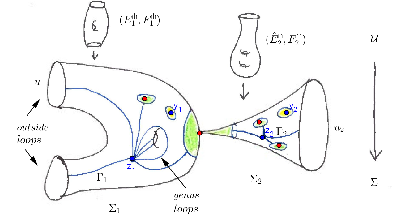
Figure 2. Critical set and the cell models for $({\cal Z},{\cal C})$ and $({\cal Y},{\cal B})$.

3.4. The CW-complex structure of $({\cal Z},{\cal C})$

The pair $({\cal Z}_{s},{\cal C}_{s})$ has the following structure of a relative CW-complex, up to homotopy. Each bundle over some circle link can be obtained from a trivial bundle over an interval by identifying the fibres above the end points via the geometric monodromy $A_{s}$. In order to obtain ${\cal Z}_{s}$ from ${\cal C}_{s}$ one can start by first attaching $n$-cells $c_{1},\ldots,c_{\mu^{\pitchfork}_{s}}$ to the fibre $F^{\pitchfork}_{s}$ in order to kill the $\mu^{\pitchfork}_{s}$ generators of $H_{n-1}(F^{\pitchfork}_{s})$ at the identified ends, and next by attaching $(n+1)$-cells $e_{1},\ldots,e_{\mu^{\pitchfork}_{s}}$ to the preceding $n$-skeleton. The attaching of some $(n+1)$-cell goes as follows: consider some $n$-cell $a$ of the $n$-skeleton and take the cylinder $I\times a$ as an $(n+1)$-cell. Fix an orientation of the circle link, attach the base $\{0\}\times a$ over $a$, then follow the circle bundle in the fixed orientation by the monodromy $A_{s}$ and attach the end $\{1\}\times a$ over $A_{s}(a)$. At the level of the cell complex, the boundary map of this attaching identifies to $A_{s}-I:{\mathbb{Z}}^{\mu^{\pitchfork}_{s}}\to{\mathbb{Z}}^{\mu^{\pitchfork}_{s}}$.

3.5. The CW-complex structure of $({\cal Y},{\cal B})$

The curve $\Sigma$ has as boundary components the intersection $\partial B\cap\Sigma$ with the Milnor ball. They are all topological circles. We denote them with $u\in U_{i}$, $U:=\cup_{i}U_{i}$ and call them outside loops. Note that over any such loop $u\in U_{i}$ we have a local system monodromy $A_{u}:{\mathbb{Z}}^{\mu^{\pitchfork}_{i}}\rightarrow{\mathbb{Z}}^{\mu^{\pitchfork}_{i}}$. In fact this monodromy did not change in the admissible deformation from $\hat{f}$ to $f$.

For technical reasons we introduce one more puncture $y_{i}$ on $\Sigma_{i}$ and next redefine $\Sigma^{*}_{i}:=\Sigma\setminus(Q\cup\{y_{i}\})$ Moreover we use notations $({\cal X}_{y},{\cal A}_{y})$ and $({\cal Z}_{y},{\cal C}_{y})$. We choose the following sets of loops in $\Sigma_{i}$:

• the $2g_{i}$ loops (called genus loops in the following) which are generators of $\pi_{1}$ of the normalization $\tilde{\Sigma}_{i}$ of $\Sigma_{i}$, where $g_{i}$ denotes the genus of this normalization (which is a Riemann surface with boundary),

• the loops $s$ around the special points $q\in Q_{i}$,

• the outside loops,

and define $W_{i}=G_{i}\sqcup S_{i}\sqcup U_{i}$ and $W=\sqcup W_{i}$. By enlarging “the hole” defined by the puncture $y_{i}$, we retract $\Sigma^{*}_{i}$ to some configuration of loops connected by non-intersecting paths to some point $z_{i}$, denoted by $\Gamma_{i}$ (see Figure 2). The number of loops is $\#W_{i}=2g_{i}+\tau_{i}+\gamma_{i}$, where $\tau_{i}:=\#U_{i}$ and $\gamma_{i}:=\sum_{q\in Q_{i}}\#S_{q}$. Note that $\tau_{i}>0$ since there must be at least one outside loop.

Each pair $({\cal Y}_{i},{\cal B}_{i})$ is then homotopy equivalent (by retraction) to the pair $(\pi_{\Sigma}^{-1}(\Gamma_{i}),{\cal B}\cap\pi_{\Sigma}^{-1}(\Gamma_{i}))$. We endow the latter with the structure of a relative CW-complex as we did with $({\cal Z},{\cal C})$ at §3.4, namely for each loop the similar CW-complex structure as we have defined above for some pair $({\cal Z}_{s},{\cal C}_{s})$. The difference is that the pairs $({\cal Z}_{s},{\cal C}_{s})$ are disjoint whereas in $\Sigma^{*}_{i}$ the loops meet at a single point $z_{i}$. We thus take as reference the transversal fibre $F^{\pitchfork}_{i}={\cal B}\cap\pi_{\Sigma}^{-1}(z_{i})$ above this point, namely we attach the $n$-cells (thimbles) only once to this single fibre in order to kill the $\mu^{\pitchfork}_{i}$ generators of $H_{n-1}(F^{\pitchfork}_{i})$. The $(n+1)$-cells of $({\cal Y}_{i},{\cal B}_{i})$ correspond to the fibre bundles over the loops in the bouquet model of $\Sigma^{*}_{i}$. Over each loop, one attaches a number of $\mu^{\pitchfork}_{i}$ $(n+1)$-cells to the fixed $n$-skeleton described before, more precisely one $(n+1)$-cell over one $n$-cell generator of the $n$-skeleton. We extend for $w\in W$ the notation $({\cal Z}_{g},{\cal C}_{g})$ to genus loops and $({\cal Z}_{u},{\cal C}_{u})$ to outside loops, although they are not contained in $({\cal Z},{\cal C})$ but in $({\cal Y},{\cal B})$.

Here the attaching map of the $(n+1)$-cells corresponding to the bundle over a genus loop, or over an outer loop, can be identified with $A_{g}-I:{\mathbb{Z}}^{\mu^{\pitchfork}_{i}}\to{\mathbb{Z}}^{\mu^{\pitchfork}_{i}}$, or with $A_{u}-I:{\mathbb{Z}}^{\mu^{\pitchfork}_{i}}\to{\mathbb{Z}}^{\mu^{\pitchfork}_{i}}$, respectively. We have seen that the monodromy $A_{u}$ over some outer loop indexed by $u\in U_{i}$ is necessarily one of the vertical monodromies of the original function $\hat{f}$.

From this CW-complex structure we get the following precise description in terms of the monodromies of the transversal local system, the proof of which is similar to that of [ST2, Lemma 4.4]:

Lemma 3.2.

1. $H_{k}({\cal Y},{\cal B})=\oplus_{i\in I}H_{k}({\cal Y}_{i},{\cal B}_{i})$ and this is $=0$ for $k\neq n,n+1.$

2. $H_{n}({\cal Y}_{i},{\cal B}_{i})\simeq{\mathbb{Z}}^{\mu^{\pitchfork}_{i}}/\langle{\mathrm{Im\hskip 1.0pt}}(A_{w}-I)\mid w\in W_{i}\rangle$,

3. $\chi({\cal Y}_{i},{\cal B}_{i})=(-1)^{n-1}(2g_{i}+\tau_{i}+\gamma_{i}-1)\mu^{\pitchfork}_{i}$.

$\square$

If we apply $\chi$ to (3.3) and (3.4) and take into account that $\chi({\cal Z},{\cal C})=0$, we get:
$\chi(E,F)=\chi({\cal X},{\cal A})+\chi({\cal Y},{\cal B})+\sum_{r}\chi(E_{r},F_{r})$. From this we derive the Euler characteristic of the Milnor fibre $F$:

Proposition 3.3.

$$\chi(F)=1+\sum_{q\in Q}(\chi({\cal A}_{q})-1)+(-1)^{n}\sum_{i\in I}(2g_{i}+\tau_{i}+\gamma_{i}-2)\mu^{\pitchfork}_{i}+(-1)^{n}\sum_{r\in R}\mu_{r}.$$

$\square$

Proposition 3.4.

The relative Mayer-Vietoris sequence (3.4) is trivial except of the following 6-terms sequence:

(3.7) $$\begin{array}[]{l}\ \ \ \ 0\to H_{n+1}({\cal Z},{\cal C})\to H_{n+1}({\cal X},{\cal A})\oplus H_{n+1}({\cal Y},{\cal B})\to H_{n+1}({\cal X}\cup{\cal Y},{\cal A}\cup{\cal B})\to\\ \ \ \ \ \ \to H_{n}({\cal Z},{\cal C})\stackrel{{\scriptstyle j}}{{\to}}H_{n}({\cal X},{\cal A})\oplus H_{n}({\cal Y},{\cal B})\to H_{n}({\cal X}\cup{\cal Y},{\cal A}\cup{\cal B})\to 0.\end{array}$$

$\square$

Proof.

Lemma 3.1, §3.2 and Lemma 3.2 show that the terms $H_{*}({\cal X},{\cal A})$, $H_{*}({\cal Y},{\cal B})$ and $H_{*}({\cal Z},{\cal C})$ of the Mayer-Vietoris sequence (3.4) are concentrated only in dimensions $n$ and $n+1$. Following (3.3) and since $\tilde{H}_{*}(F)$ is concentrated in levels $n-1$ and $n$, we obtain that $H_{n+2}({\cal X}\cup{\cal Y},{\cal A}\cup{\cal B})=0$. ∎

The first 3 terms of (3.7) are free. By the decomposition (3.3), in order to find the homology of $F$ we thus need to compute $H_{k}({\cal X}\cup{\cal Y},{\cal A}\cup{\cal B})$ for $k=n,n+1$, since the others are zero. In the remainder of this paper we find information only about $H_{n}({\cal X}\cup{\cal Y},{\cal A}\cup{\cal B})$. The knowledge of its dimension is then enough for determining $H_{n}(F)$, by only using the Euler characteristic formula (Prop. 3.3).

4. The homology group $H_{n-1}(F)$

We concentrate on the term $H_{n}({\cal X}\cup{\cal Y},{\cal A}\cup{\cal B})\simeq\tilde{H}_{n-1}(F)$. We need the relative version of the “variation-ladder”, an exact sequence found in [Si4, Theorem 5.2, p. 456-457]. This sequence has an important overlap with our relative Mayer-Vietoris sequence (3.7).

Proposition 4.1.

[ST2, Proposition 5.2] For any point $q\in Q$, the sequence

$$\begin{array}[]{l}0\rightarrow H_{n+1}({\cal A}_{q},\partial_{2}{\cal A}_{q})\rightarrow\mathop{\oplus}_{s\in S_{q}}H_{n+1}({\cal Z}_{s},{\cal C}_{s})\rightarrow H_{n+1}({\cal X}_{q},{\cal A}_{q})\rightarrow\\ \ \ \ \ \ \rightarrow H_{n}({\cal A}_{q},\partial_{2}{\cal A}_{q})\rightarrow\ \mathop{\oplus}_{s\in S_{q}}H_{n}({\cal Z}_{s},{\cal C}_{s})\ \rightarrow\ H_{n}({\cal X}_{q},{\cal A}_{q})\ \rightarrow\ 0\end{array}$$

is exact for $n\geq 2$. $\square$

4.1. The image of $j$

We focus on the map $j=j_{1}\oplus j_{2}$ which occurs in the 6-term exact sequence (3.7), more precisely on the following exact sequence:

(4.1) $$H_{n}({\cal Z},{\cal C})\stackrel{{\scriptstyle j}}{{\to}}H_{n}({\cal X},{\cal A})\oplus H_{n}({\cal Y},{\cal B})\to H_{n}(F)\to 0.$$

since we have the isomorphism:

(4.2) $$H_{n-1}(F)\simeq\mathop{{\mathrm{coker}}}\nolimits j.$$

Therefore full information about $j$ makes is possible to compute $H_{n-1}(F)$. But although $j$ is of geometric nature, this information is not always easy to obtain. Below we treat its two components in separately. After that we will make two statements (Theorems 4.4 and 4.6) of a more general type.

4.1.1. The first component $j_{1}:H_{n}({\cal Z},{\cal C})\to H_{n}({\cal X},{\cal A})$

Note that, as shown above, we have the following direct sum decompositions of the source and the target:

$$\begin{array}[]{l}H_{n}({\cal Z},{\cal C})=\oplus_{q\in Q}\oplus_{s\in S_{q}}H_{n}({\cal Z}_{s},{\cal C}_{s})\oplus\oplus_{i\in I}H_{n}({\cal Z}_{y_{i}},{\cal C}_{y_{i}}),\\ H_{n}({\cal X},{\cal A})=\oplus_{q\in Q}H_{n}({\cal X}_{q},{\cal A}_{q})\oplus\oplus_{i\in I}H_{n}({\cal X}_{y_{i}},{\cal A}_{y_{i}}).\end{array}$$

As shown in Proposition 4.1, at the special points $q\in Q$ we have surjections: $\mathop{\oplus}_{s\in S_{q}}H_{n}({\cal Z}_{s},{\cal C}_{s})\rightarrow H_{n}({\cal X}_{q},{\cal A}_{q})$ and moreover $H_{n}({\cal Z}_{y},{\cal C}_{y})\rightarrow H_{n}({\cal X}_{y},{\cal A}_{y})$ is an isomorphism. We conclude to the surjectivity of the morphism $j_{1}$ and to the cancellation of the contribution of the points $y_{i}$ for $\mathop{{\mathrm{coker}}}\nolimits j$.

4.1.2. The second component $j_{2}:H_{n}({\cal Z},{\cal C})\to H_{n}({\cal Y},{\cal B})$

Both sides are described with a relative CW-complex as explained in §3.5. At the level of $n$-cells there are $\mu^{\pitchfork}_{s}$ $n$-cell generators of $H_{n}({\cal Z}_{s},{\cal C}_{s})$ for each $s\in S_{q}$ and any $q\in Q$. Each of these generators is mapped bijectively to the single cluster of $n$-cell generators attached to the reference fibre $F^{\pitchfork}_{i}$ (which is the fibre above the common point $z_{i}$ of the loops). The restriction ${j_{2}}_{|}:H_{n}({\cal Z}_{s},{\cal C}_{s})\to H_{n}({\cal Y}_{i},{\cal B}_{i})$ is a projection for any loop $s$ in $\Sigma_{i}$ and $q\in Q_{i}$, or if instead of $s$ we have $y_{i}$, since we add extra relations to ${\mathbb{Z}}^{\mu^{\pitchfork}}/\langle A_{s}-I\rangle$ in order to get ${\mathbb{Z}}^{\mu^{\pitchfork}_{i}}/\langle{\mathrm{Im\hskip 1.0pt}}(A_{w}-I)\mid w\in W_{i}\rangle=H_{n}({\cal Y}_{i},{\cal B}_{i})$. We summarize the above surjections as follows:

Lemma 4.2.

(“Strong surjectivity”)

1. Both $j_{1}$ and $j_{2}$ are surjective.

2. The restriction ${j_{2}}_{|}:H_{n}({\cal Z}_{s},{\cal C}_{s})\rightarrow H_{n}({\cal Y}_{i},{\cal A}_{i})$ is surjective for any $s\in S_{q}$ such that $q\in Q\cap\Sigma_{i}$.

3. The restriction $j_{1}|\oplus_{s\in S_{q}}H_{n}({\cal Z}_{s},{\cal C}_{s})\rightarrow H_{n}({\cal X}_{q},{\cal A}_{q})$ is surjective, for any $q\in Q$.

$\square$

Corollary 4.3.

1. If the restriction ${j_{2}}|\mathop{{\mathrm{ker}}}\nolimits j_{1}$ is surjective, then $j$ is surjective.

2. If for each $i\in I$ there exists $q_{i}\in Q\cap\Sigma_{i}$ and some $s\in S_{q_{i}}$ such that $H_{n}({\cal Z}_{s},{\cal C}_{s})\subset\mathop{{\mathrm{ker}}}\nolimits j_{1}$ then $j$ is surjective.

$\square$

Proof.

(a). More generally, let $j_{1}:M\to M_{1}$ and $j_{2}:M\to M_{2}$ be morphisms of ${\mathbb{Z}}$-modules such that $j_{1}$ is surjective and consider the direct sum of them $j:=j_{1}\oplus j_{2}$. We assume that the restriction ${j_{2}}|\mathop{{\mathrm{ker}}}\nolimits j_{1}$ is surjective onto $M_{2}$ and want to prove that $j$ is surjective.

Let then $(a,b)\in M_{1}\oplus M_{2}$. There exists $x\in M$ such that $j_{1}(x)=a$, by the surjectivity of $j_{1}$. Let $b^{\prime}:=j_{2}(x)$. By our surjectivity assumption there exists $y\in\mathop{{\mathrm{ker}}}\nolimits j_{1}$ such that $j_{2}(y)=b-b^{\prime}$. Then $j(x+y)=a+b$, which proves the surjectivity of j.

(b). follows immediately from Lemma 4.2(b) and from the above (a). ∎

4.2. Effect of local system monodromies on $H_{n}(F)$

Recall that $w\in W_{i}$ stands for some loop $s,g,u$ in $\Sigma_{i}^{*}$.

Theorem 4.4.

1. If there is $w\in W_{i}$ such that $\det(A_{w}-I)\not=0$ then $\dim H_{n}({\cal Y}_{i},{\cal B}_{i})=0$.
   If such $w\in W_{i}$ exists for any $i\in I$, then $b_{n-1}(F)=0$.

2. If there is $w\in W_{i}$ such that $\det(A_{w}-I)=\pm 1$ then $H_{n}({\cal Y}_{i},{\cal B}_{i})=0$.
   If such $w\in W_{i}$ exists for any $i\in I$, then $H_{n-1}(F)=0$.

3. The following upper bound holds:

   $$b_{n-1}(F)\leq\sum_{i\in I}\min_{w\in W_{i}}\dim\mathop{{\mathrm{coker}}}\nolimits(A_{w}-I)\leq\sum_{i\in I}\mu^{\pitchfork}_{i}.$$

Proof.

By Lemma 3.2(b). we have $H_{n}({\cal Y}_{i},{\cal B}_{i})\simeq{\mathbb{Z}}^{\mu^{\pitchfork}_{i}}/\langle{\mathrm{Im\hskip 1.0pt}}(A_{w}-I)\mid w\in W_{i}\rangle$, thus the first parts of (a) and (b) follow. For the second part of (a), we have that $\dim H_{n}({\cal Y},{\cal B})=0$, hence $\mathrm{corank\hskip 2.0pt}j=\mathrm{corank\hskip 2.0pt}j_{1}=0$. For the second part of (b), we have that $H_{n}({\cal Y},{\cal B})=0$ and the surjectivity of the map $j$ of (4.1) is equivalent to the fact that $j_{1}$ is surjective.

To prove (c), we consider homology groups with coefficients in ${\mathbb{Q}}$. Since $j_{1}$ is surjective, the image of $j$ contains all the generators of $H_{n}({\cal X},{\cal A};{\mathbb{Q}})$. Hence $\dim\mathop{{\mathrm{coker}}}\nolimits j\leq\dim H_{n}({\cal Y},{\cal B})$. ∎

Remark 4.5.

Notice the effect of the strongest bound in the above theorem. On each $\Sigma_{i}$ one could take an optimal loop, e.g. one with $\det(A_{w}-I)=\pm 1$. Since in the deformed case there may be less branches $\Sigma_{i}$, and more special points and hence more vertical monodromies, these bounds may become much stronger than those in [Si4].

4.3. Effect of the local fibres ${\cal A}_{q}$

Theorem 4.6.

Let $n\geq 2$.

1. Assume that for each irreducible 1-dimensional component $\Sigma_{i}$ of $\Sigma$ there is a special singularity $q\in Q_{i}$ such that the $(n-1)$th homology group of its Milnor fibre is trivial, i.e. $H_{n-1}({\cal A}_{q})=0$. Then $H_{n-1}(F)=0$.

   If in the above assumption we replace $H_{n-1}({\cal A}_{q})=0$ by $b_{n-1}({\cal A}_{q})=0$, then we get $b_{n-1}(F)=0$.

2. Let $Q^{\prime}:=\{q_{1},\ldots,q_{m}\}\subset Q$ be some (minimal) subset of special points such that each branch $\Sigma_{i}$ contains at least one of its points. Then:

   $$b_{n-1}(F)\leq\dim H_{n}({\cal X}_{q_{1}},{\cal A}_{q_{1}})+\cdots+\dim H_{n}({\cal X}_{q_{m}},{\cal A}_{q_{m}}).$$

Proof.

(a). We use (4.1) in order to estimate the dimension of the image of $j=j_{1}\oplus j_{2}$. If there is a $q\in Q$ such that $H_{n}({\cal X}_{q},{\cal A}_{q})=0$ then $\mathop{{\mathrm{ker}}}\nolimits j_{1}$ contains $\oplus_{s\in S_{q}}H_{n}({\cal Z}_{s},{\cal C}_{s})$. Since $Q^{\prime}$ meets all components $\Sigma_{i}$, statement (a) follows from Corollary 4.3(b). The second claim of (a) follows by considering homology over ${\mathbb{Q}}$.

(b). We work again with homology over ${\mathbb{Q}}$. We consider the projection on a direct summand $\pi:H_{n}({\cal X},{\cal A})\to\oplus_{q\not\in Q^{\prime}}H_{n}({\cal X}_{q},{\cal A}_{q})$ and the composed map $J_{1}:=\pi\circ j_{1}$. Then the restriction $j_{2}|\mathop{{\mathrm{ker}}}\nolimits J_{1}$ is surjective, which by Corollary 4.3(a), means that $J_{1}\circ j_{2}$ is surjective. Then the result follows from the obvious inequality $\dim({\mathrm{Im\hskip 1.0pt}}J_{1}\circ j_{2})\leq\dim{\mathrm{Im\hskip 1.0pt}}j$ by counting dimensions. ∎

Remark 4.7.

Also here we have the effect of the strongest bound. This works at best if one chooses an optimal or minimal $Q^{\prime}$ (see e.g. Figure 3). In the irreducible case, $H_{n-1}({\cal A}_{q})=0$ for at least one $q\in Q$ already implies the triviality $H_{n-1}(F)=0$.

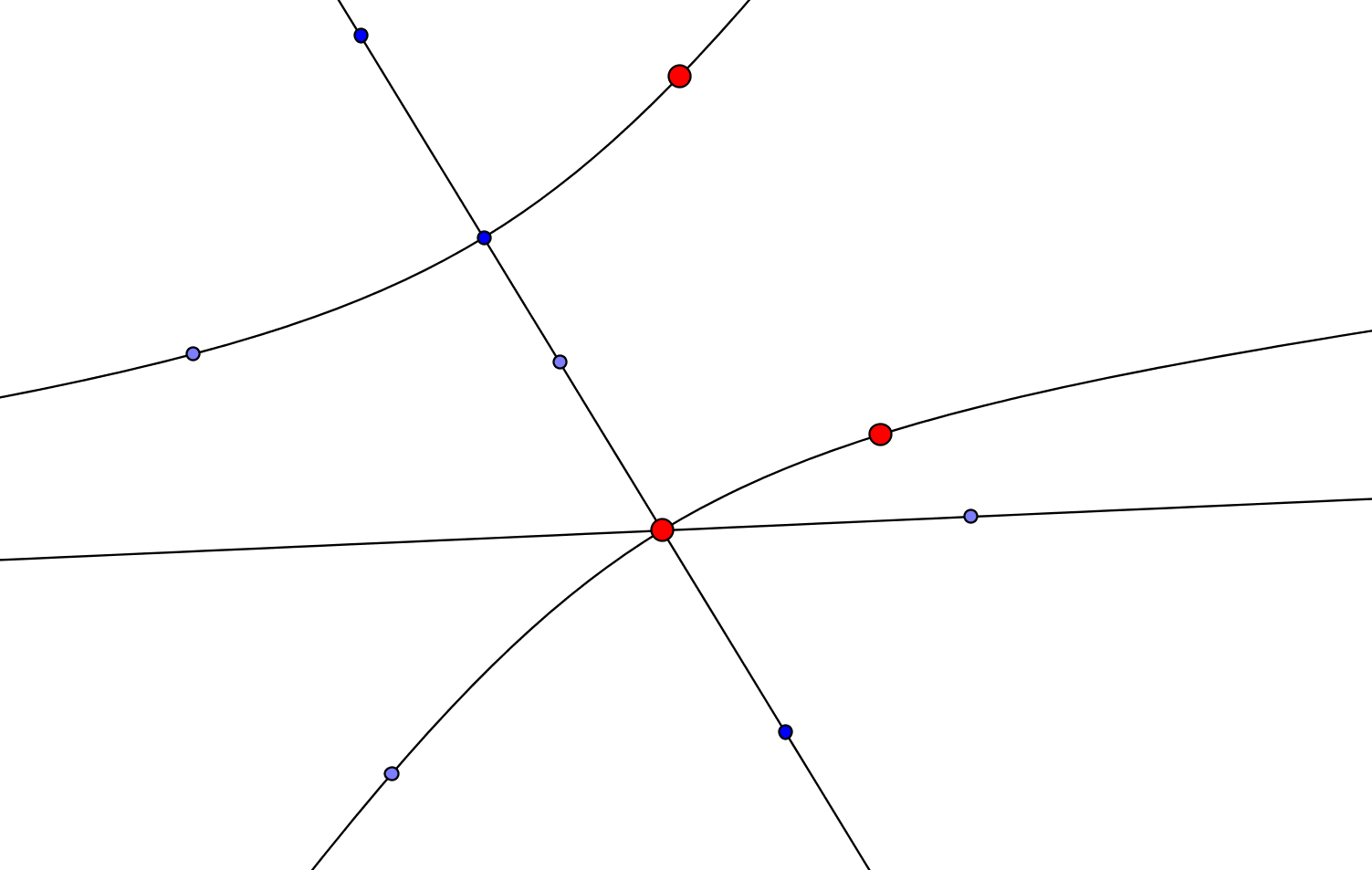
Figure 3. A choice of Q-points

Corollary 4.8.

(Bouquet Theorem) If $n\geq 3$ and

• If for any $i\in I$ there is $w\in W_{i}$ such that $\det(A_{w}-I)=\pm 1$, or

• If for every $\Sigma_{i}$ there is a special singularity $q\in Q_{i}$ such that $H_{n-1}({\cal A}_{q})=0$

then

$$F\stackrel{{\scriptstyle{\mathrm{ht}}}}{{\simeq}}S^{n}\vee\cdots\vee S^{n}.$$

Proof.

From Theorems (4.4b) or (4.6a) follows $H_{n-1}(F)=0$. Since $F$ is a simply connected $n$-dimensional CW-complex the statement follows from Milnor’s argument ([Mi], theorem 6.5) and Whitehead’s theorem. ∎

5. Examples

5.1. Singularities with transversal type $A_{1}$

The case when $\Sigma$ is a smooth line was considered in [Si1] and later generalized to $\Sigma$ a 1-dimensional complete intersection (icis) [Si2]. It uses an admissible deformation with only $D_{\infty}$-points. The main statement is:

• $F\stackrel{{\scriptstyle{\mathrm{ht}}}}{{\simeq}}S^{n-1}$ if $\#D_{\infty}=0$,

• $F\stackrel{{\scriptstyle{\mathrm{ht}}}}{{\simeq}}S^{n}\vee\cdots\vee S^{n}$ else.

Since $D_{\infty}$-points have $H_{n-1}({\cal A}_{q})=0$, our Theorem 4.6 provides a proof of this statement on the level of homology. If $\Sigma$ is not an icis, more complicated situations occur. For details about the following example, cf [Si2].

• $f=xyz$, called $T_{\infty,\infty,\infty}$ : $\Sigma$ is the union of 3 coordinate axis. $F\cong S^{1}\times S^{1}$, so $b_{1}(F)=2$, $b_{2}(F)=1$ and all $A_{u}=I$.

• $f=x^{2}y^{2}+y^{2}z^{2}+x^{2}z^{2}$ has $F\cong S^{2}\vee\cdots\vee S^{2}$. The admissible deformation $f_{s}=f+sxyz$ has the same $\Sigma$ as $f=xyz$, but now with 3 $D_{\infty}$-points on each component of $\Sigma$ and one $T_{\infty,\infty,\infty}$-point in the origin. Our Theorem 4.6 therefore states $H_{1}(F)=0$. A real picture of $f_{s}=0$ contains the Steiner surface, for $s\not=0$ small enough (Figure 4(a)). That $H_{2}(F)={\mathbb{Z}}^{15}$ follows from $\chi(F)=16$ computed via Proposition 3.3.

  

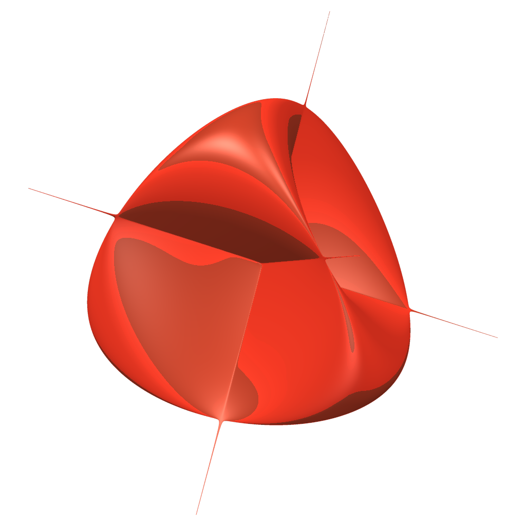
  (a) Steiner Surface

  

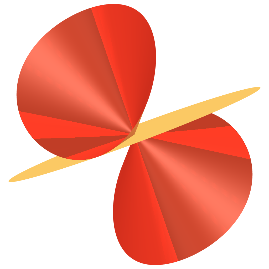
  (b) Singularity $F_{1}A_{3}$

  

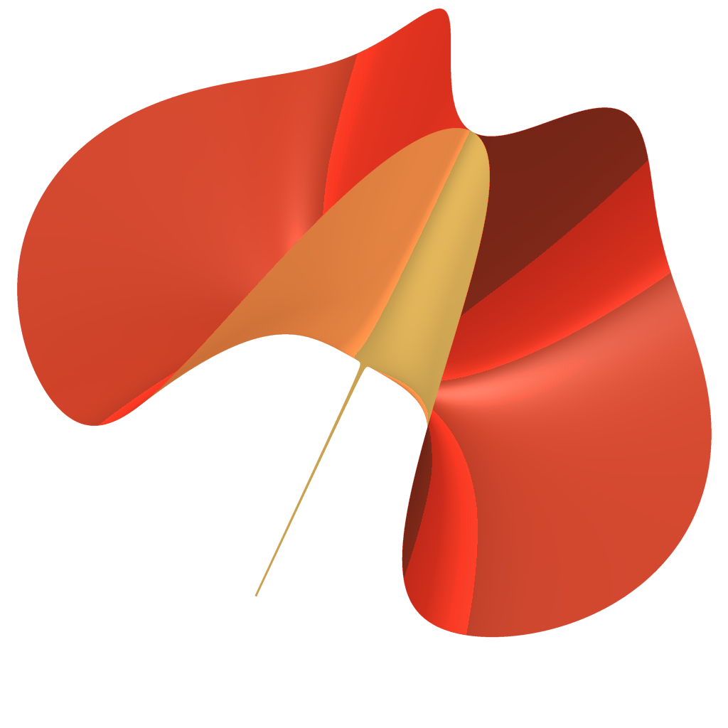
  (c) Singularity $F_{2}A_{3}$

  Figure 4. Several Singularites (produced with Surfer software)

5.2. Transversal type $A_{2},A_{3},D_{4},E_{6},E_{7},E_{8}$, De Jong List

In [dJ] there is a detailed description of singularities with singular set a smooth line and transversal type $A_{2},A_{3},D_{4},E_{6},E_{7},E_{8}$. His list illustrates and confirms our statements at the level of homology.

We will treat below in more detail the case $f:{\mathbb{C}}^{3}\to{\mathbb{C}}$ with transversal type $A_{3}$. (By adding squares, this also illustrates $f:{\mathbb{C}}^{n+1}\to{\mathbb{C}}$.) Any singularity of this type can be deformed into

• : $f=xz^{2}+y^{2}z\;;\;F\stackrel{{\scriptstyle{\mathrm{ht}}}}{{\simeq}}S^{1}$ (figure 4(b))

• : $f=xy^{4}+z^{2}\;;\;F\stackrel{{\scriptstyle{\mathrm{ht}}}}{{\simeq}}S^{2}$ (figure 4(c))

De Jong’s observation is that for any line singularity of transversal type $A_{3}$we have:

• $F\stackrel{{\scriptstyle{\mathrm{ht}}}}{{\simeq}}S^{n-1}\vee S^{n}\cdots\vee S^{n}$ if $\#F_{2}A_{3}=0$,

• $F\stackrel{{\scriptstyle{\mathrm{ht}}}}{{\simeq}}S^{n}\vee\cdots\vee S^{n}$ else.

In homology, (b) follows directly from our concentration result 4.6. The homology version of (a) takes more efforts. We demonstrate this in the following example only. First we mention that for $F_{1}A_{3}$ the vertical monodromy $A$ is equal to the Milnor monodromy $h$. This follows from the fact that $f=xz^{2}+y^{2}z$ is homogeneous of degree $d=3$ and Steenbrink’s remark [St] that $Ah^{d}=I$ and that $h^{4}=I$. The matrix of $h$ is:

$$\begin{pmatrix}1&1&\ 1\\ -1&0&0\\ 0&-1&0\end{pmatrix}$$

It follows: $\mathop{{\mathrm{ker}}}\nolimits(h-I)={\mathbb{Z}}$ ; Im $(h-I)={\mathbb{Z}}^{2}$ and $\mathop{{\mathrm{coker}}}\nolimits(h-I)={\mathbb{Z}}.$

Next consider as example the deformation $f:=f_{s}=(x^{k}-s)z^{2}+yz^{2}+y^{2}z$ for some fixed small enough $s\not=0$, which has transversal type $A_{3}$. This deformation has $\#F_{1}A_{3}=k$ and $\#F_{2}A_{3}=0$ and moreover one isolated critical point of type $A_{k}$. We compare now the fundamental sequence for $j$ in case $F_{1}A_{3}$ and $f$ respectively:

(5.1) $$j=j_{1}\oplus j_{2}:{\mathbb{Z}}\rightarrow{\mathbb{Z}}\oplus{\mathbb{Z}}\rightarrow H_{n-1}(F_{F_{1}A_{3}})={\mathbb{Z}}\rightarrow 0$$

(5.2) $$j=j_{1}\oplus j_{2}:{\mathbb{Z}}^{k}\rightarrow{\mathbb{Z}}^{k}\oplus{\mathbb{Z}}\rightarrow H_{n-1}(F_{f})={\mathbb{Z}}\rightarrow 0$$

The map $j_{2}$ for $f$ is as follows:

$\oplus_{s}H_{n}({\cal Z}_{s},{\cal C}_{s})={\mathbb{Z}}^{k}=\oplus_{s}{\mathbb{Z}}^{3}/\langle h-I\rangle\to{\mathbb{Z}}^{3}/\langle h-I,A_{u}-I\rangle=H_{n}({\cal Y},{\cal B})$. It is the sum of components which are isomorphism on each factor ${\mathbb{Z}}$. Note that for the outside loop $u$ we have $A_{u}-I=(h-1)(h^{k-1}+\cdots+h+I)$ since $A_{u}=A_{s_{1}}\circ\cdots\circ A_{s_{k}}=h^{k}$ (all $A_{s}$ are equal to $h$).
We conclude $H_{1}(F_{f})={\mathbb{Z}}$. Next $H_{2}(F_{f})={\mathbb{Z}}^{3k-1}$ follows from $\chi(F_{f})=3k-1$ computed via Proposition 3.3.

We illustrate this example with Figures 5(a) and 5(b).

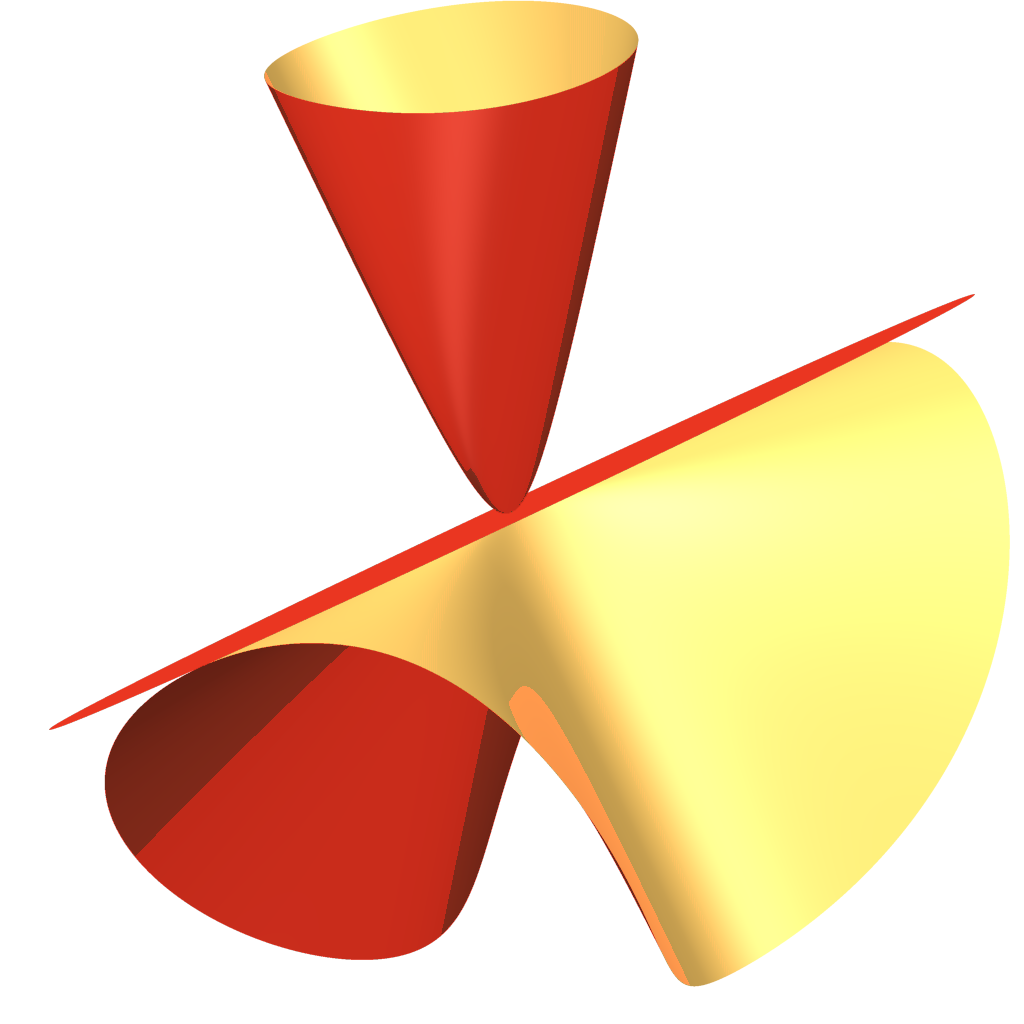
(a) Original surface

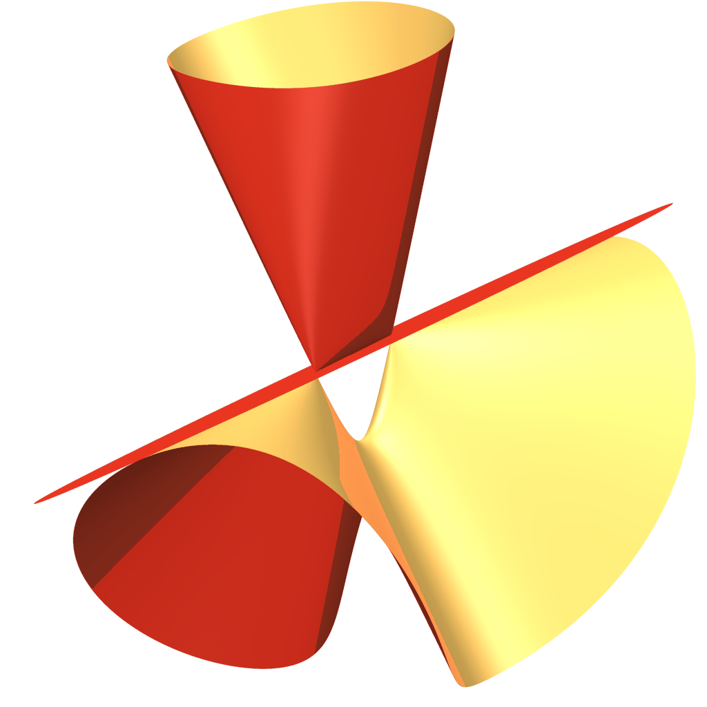
(b) Deformed surface

Figure 5. Deformation $f_{s}=(x^{k}-s)z^{2}+yz^{2}+y^{2}z$, (produced with Surfer software)

5.3. More general types

We show next that the above method is not restricted to the De Jong classes. Consider $f=z^{2}x^{m}-z^{m+2}+zy^{m+1}$. It has the properties: $F\simeq S^{1}$ ; $\Sigma$ is smooth; transversal type is $A_{2m+1}$; $A=h^{m}$, where $h$ is the Milnor monodromy of $A_{2m+1}$.

Note that $\dim\mathop{{\mathrm{ker}}}\nolimits(A-I)\geq 1$, and $=1$ in many cases, e.g. $m=2,3,4,5$. This function $f$ appears as ‘building block’ in the following deformation:
$g_{s}=z^{2}(x^{2}-s)^{m}-z^{m+2}+zy^{m+1}.$
This deformation contains two special points of the type $f$ (and no others, except isolated singularities). If one applies the same procedure as above one gets $b_{1}(G)=1$ where $G$ is the Milnor fibre of $g_{0}$. Details are left to the reader.

Remark 5.1.

The fact that the first Betti number of the Milnor fibre is non-zero can also be deduced from Van Straten’s [vS, Theorem 4.4.12]: Let $f:({\mathbb{C}}^{3},0)\to({\mathbb{C}},0)$ be a germ of a function without multiple factors, let $F$ be the Milnor fibre of $f$. Then

$$b_{1}(F)\geq\#\mbox{\rm\{irreducible components of}\;f=0\}.$$

5.4. Deformation with triple points

Let $f_{s}=xyz(x+y+z-s)$. This defines a deformation of a central arrangement with 4 hyperplanes. We get $\Sigma_{i}={\mathbb{P}}^{1}$ (6 copies). There are 4 triple points $T_{\infty,\infty,\infty}$ and one $A_{1}$-point. The maps $j_{1,q}:{\mathbb{Z}}^{3}\to{\mathbb{Z}}^{2}$ can be described by $j_{1,q}(a,b,c)=(a+c,b+c)$. The map $j_{2}$ restricts to an isomorphism ${\mathbb{Z}}\to{\mathbb{Z}}$ on each component. We have all information of the resulting map $j:{\mathbb{Z}}^{12}\to{\mathbb{Z}}^{14}$ up to the signs of the isomorphisms. From this we get $H_{1}(F;{\mathbb{Z}}_{2})={\mathbb{Z}}_{2}^{3}$. Compare with the dissertation [Wi], where Williams showed in particular that $H_{1}(F;{\mathbb{Z}})={\mathbb{Z}}^{3}$.

5.5. The class of singularities with $b_{n}=0$

Most of the singularities above have $b_{n-1}=0$ or small. What happens if $b_{n}=0$ ? Examples are the product of an isolated singularity with a smooth line (such as $A_{\infty})$ and some of the functions mentioned above (e.g. $F_{2}A_{3}$). Very few is known about this class. We can show the following “non-splitting property” w.r.t. isolated singularities:

Proposition 5.2.

If $\hat{f}$ has the property, that $b_{n}(\hat{F})=0$, then any admissible deformation has no isolated critical points.

Proof.

Note that in 3.3 we have $H_{*}(E,F)=0$. It follows, that $H_{*}({\cal X}\cup{\cal Y},{\cal A}\cup{\cal B})=0$ and $\oplus_{r\in R}H_{*}(E_{r},F_{r})=0$. Therefore the set $R$ is empty. ∎

References

- [1]
- [dJ] T. de Jong, Some classes of line singularities. Math. Z. 198, (1988) 493–517.
- [MS] D.B. Massey, D. Siersma, Deformation of polar methods. Ann. Inst. Fourier, Grenoble, 42, (1992), 737-778.
- [Mi] J. Milnor, Singular points of complex hypersurfaces. Ann. of Math Studies 61 (1968) Princeton Univ. Press.
- [NS] A. Némethi, À. Szilàrd, Milnor Fiber Boundary of a Non-isolated Surface Singularity Lecture Notes in Mathematics 2037, Springer Verlag, 2012.
- [Ra] R. Randell, On the topology of non-isolated singularities. In: Geometric Topology (Proc. 1977 Georgia Topology Conference), Ac. Press, New York (1979) 445–473.
- [Si1] D. Siersma, Isolated line singularities. Singularities, Part 2 (Arcata, Calif., 1981), 485–496, Proc. Sympos. Pure Math., 40, Amer. Math. Soc., Providence, RI, 1983.
- [Si2] D. Siersma, Singularities with critical locus a 1-dimensional complete intersection and transversal type ., Topology and its Applications 27 (1987) 51–73.
- [Si3] D. Siersma, Quasi-homogeneous singularities with transversal type . Singularities (Iowa City, IA, 1986), 261–294, Contemp. Math., 90, Amer. Math. Soc., Providence, RI, 1989.
- [Si4] D. Siersma, Variation mappings on singularities with a 1-dimensional critical locus. Topology 30 (1991), no. 3, 445–469.
- [Si5] D. Siersma, The vanishing topology of non isolated singularities. New developments in singularity theory (Cambridge, 2000), 447–472, NATO Sci. Ser. II Math. Phys. Chem., 21, Kluwer Acad. Publ., Dordrecht, 2001.
- [ST1] D. Siersma, M. Tibăr, Betti numbers of polynomials, Mosc. Math. J. 11 (2011), no. 3, 599–615.
- [ST2] D. Siersma, M. Tibăr, Vanishing homology of projective hypersurfaces with 1-dimensional singularities, arXiv 1411.2640.
- [St] J.H.M. Steenbrink, The spectrum of hypersurface singularities, Astérisque 179-180, 163-184 (1989).
- [Ti] M. Tibăr, The vanishing neighbourhood of non-isolated singularities. Israel J. Math. 157 (2007), 309–322.
- [vS] D. van Straten, Weakly normal surface singularities and their improvements. Dissertation Rijksuniversiteit Leiden, 1987.
- [Wi] K.J. Williams, The Milnor fiber associated to an arrangement of hyperplanes. Dissertation The University of Iowa, Iowa, 2011.
- [Yo] I.N. Yomdin, Complex surfaces with a one-dimensional set of singularities. Sibirsk. Mat. Z. 15 (1974), 1061–1082, 1181.
- [2]