Approximated Analytical Solution to
an Ebola Optimal Control Problem

Abstract

An analytical expression for the optimal control of an Ebola problem is obtained. The analytical solution is found as a first-order approximation to the Pontryagin Maximum Principle via the Euler–Lagrange equation. An implementation of the method is given using the computer algebra system Maple. Our analytical solutions confirm the results recently reported in the literature using numerical methods.

Keywords: Optimal Control; Euler–Lagrange equation; Computer Algebra; Ebola; Approximated analytical expressions.

Mathematics Subject Classification 2010: 49-04; 49K15; 92D30.

1 Introduction

The largest outbreak of Ebola virus ever recorded has been ongoing since was first confirmed in March, 2014. Ebola is a fatal disease that has claimed 7 000 lives by the end of 2014 in just Guinea, Liberia and Sierra Lione. While the Ebola outbreak has slowed down across West Africa by June 2015, every new infection continues to threaten millions of lives and bringing fear to the world. With more than 24 000 cases and almost 10 000 fatalities, this outbreak is already one of the biggest public health crises of the XXI century. Overcoming Ebola is a complex emergency, challenging not only governments and international aid organisations but also computational and life scientists and applied mathematicians [1, 3, 5, 6, 7, 8].

In a recent work by Rachah and Torres, an optimal control problem of the 2014 Ebola outbreak in West Africa was posed and numerically solved through Matlab and the ACADO toolkit [6]. See also [7] for a different model and other Matlab numerical simulations. In contrast, here we address the problem by analytical methods. The results confirm the previous numerical results, but now with a theoretical/analytical foundation. The new method is simple but envolves lengthy calculations. For this reason, a computer algebra package with the proposed method is developed in Maple.

The text is organized as follows. In Section 2 the optimal control problem is formulated. Our method is explained in Section 3 and illustrated with an example. Then, in Section 4, we apply it to the Ebola optimal control problem. We end with Section 5 of conclusions, while Appendix A provides the developed Maple code.

2 The Problem

The Ebola problem of optimal control proposed in [6] consists to determine the control function $u(\cdot)$ in such a way the objective functional given by

$$\mathcal{J}\left(u\right)=\int_{0}^{T}\!\left[I\left(t\right)+\frac{1}{2}Au\left(t\right)^{2}\right]{dt}$$ (1)

is minimized, where $A$ is a fixed nonnegative constant, when subject to the dynamic equations

$${\frac{d}{dt}}S\left(t\right)=-\beta\,S\left(t\right)I\left(t\right)-u\left(t\right)S\left(t\right)$$ (2)

$${\frac{d}{dt}}I\left(t\right)=\beta\,S\left(t\right)I\left(t\right)-\mu\,I\left(t\right)$$ (3)

$${\frac{d}{dt}}R\left(t\right)=\mu\,I\left(t\right)+u\left(t\right)S\left(t\right)$$ (4)

for all

$$t\in[0,T],$$ (5)

the given initial conditions

$$S(0)\geq 0,\quad I(0)\geq 0,\quad R(0)\geq 0,$$ (6)

and where the control values are bounded in the interval $[0,0.9]$, that is,

$$0\leq u(t)\leq 0.9.$$ (7)

Here $T$ is the duration of the application of the control (duration of the vaccination program). The constant $0.9$ is a control value that is able to eliminate the Ebola transmission according with $R_{0}<1$, where $R_{0}$ is the basic reproduction number for the system (2)–(4), and control $u$ is considered constant along all time. This control $u(t)\equiv 0.9$ is however not optimal. For this reason, we search for an optimal value of $u(t)$, $t\in[0,T]$, subject to the constraint given by (7). Note that the control $u(t)$ represents the vaccination rate at time $t$. Being the fraction of susceptible individuals vaccinated per unit of time, the value $0.9$ means that, at maximum, 90% of susceptible are vaccinated. In other words, what we assume here is that the fraction of individuals who are not vaccinated takes at least the value of 10%. This is in agreement with general experience in vaccination, where it is well recognized the impossibility to vaccinate all population. For more details on the description of the mathematical model and the meaning of the parameters, we refer the reader to the work of Rachah and Torres [6, 7]. In particular, see the scheme of the susceptible-infected-recovered model with vaccination found in Section 4.2 of [6] and the optimal control problem in Section 5 of [6], where the following parameters, initial conditions, and time horizon are considered: infection rate $\beta=0.2$; recovery rate $\mu=0.1$; at the beginning 95% of population is susceptible and 5% is already infected, that is, $S(0)=0.95$, $I(0)=0.05$ and $R(0)=0$; and $T=100$ days. Differently from previous works [6, 7], which are exclusively based on numerical methods, we address the optimal control problem (1)–(7) by using an approximated analytic method. For that we make use of the computer algebra system Maple.

3 The Method

In this section the approximated analytical method that is used in Section 4 to solve the optimal control problem (1)–(7) is explained and illustrated with an example. The idea is to use the classical calculus of variations, specifically the Euler–Lagrange equation, which is its main tool. The Euler–Lagrange equation is used with the aim to obtain a first-order approximation to the Pontryagin Maximum Principle. Typically, the Pontryagin Maximum Principle is harder to solve analytically than the Euler–Lagrange equation. In contrast, the Euler–Lagrange equations can be easily solved analytically in many interesting cases. In our work we perform an analytical experiment consisting to solve analytically the optimal control problem (1)–(7), which was previously solved numerically in [6]. As we shall see in Section 4, our approach turns out to be a good one.

Let us start with the dynamical control system

$${\frac{d}{dt}}y\left(t\right)=F\left(y\left(t\right),u\left(t\right)\right),$$ (8)

where $y(\cdot)$ is the state vector that must be controlled and $u(\cdot)$ is the control that must be applied to the system in order to minimize the functional

$$\mathcal{I}\left(u\right)=\int_{0}^{T}\left[\left({\frac{d}{dt}}u\left(t\right)\right)^{2}+\frac{1}{2}Au\left(t\right)^{2}\right]{dt},$$ (9)

where $A$ is the parameter that is determining the cost of the control and $T$ is the duration of application of the control. Comparing the objective functionals (1) and (9), we are assuming that $I(t)=(du(t)/dt)^{2}$. This is a particular case of the more general assumption

$$I(t)=a_{1}(t)u(t)+a_{2}(t)(du(t)/dt)^{2}+a_{3}(t)(du(t)/dt)^{4}+\cdots.$$ (10)

From the epidemiological point of view, given that system (2)–(4) can be considered as a black box, being the input $u(t)$ and the output $I(t)$, it is possible to think that $I(t)$ is approximately given by a series of the form (10). Given that $I(t)$ is always positive, we use even powers of $du(t)/dt$. The simplest assumption is then $I(t)=(du(t)/dt)^{2}$, which makes functional (9) to take the form of the Lagrangian for the classical harmonic oscillator. It is possible to use other forms for $I(t)$ as a function of $u(t)$ and its derivatives. For our purposes, the simplest expression $I(t)=(du(t)/dt)^{2}$ is enough. The Euler–Lagrange equation (see, e.g., [2]) associated with (9) is

$$Au\left(t\right)-2\,{\frac{d^{2}}{d{t}^{2}}}u\left(t\right)=0$$ (11)

and the solution of (11) with the conditions

$$\left\{u\left(0\right)=U_{{0}},u\left(\infty\right)=0\right\}$$ (12)

is given by

$$u\left(t\right)=U_{{0}}{{\rm e}^{-\frac{1}{2}\sqrt{2}\sqrt{A}t}}.$$ (13)

In (11) we are assuming that $u$ is of class $C^{2}$: the classical Euler–Lagrange equation is a second-order differential equation. The exact solution $u$ is not necessarily $C^{2}$, but it can always be approximated by a $C^{2}$ function. Note that our goal is to find an approximated analytical solution and not the exact one. Replacing (13) in (8), we obtain that

$${\frac{d}{dt}}y\left(t\right)=F\left(y\left(t\right),U_{{0}}{{\rm e}^{-\frac{1}{2}\sqrt{2}\sqrt{A}t}}\right).$$ (14)

Now we assume that equation (14) can be solved analytically when subject to the initial condition $y(0)=Y_{0}$. Then, formally, it is possible to write that

$$y\left(t\right)=G\left(t,A,U_{{0}},Y_{{0}}\right).$$ (15)

To determine $U_{0}$, we minimize the following functional:

$$\mathcal{K}\left(u\right)=\int_{0}^{T}\!\left[y\left(t\right)+\frac{1}{2}A\left(u\left(t\right)\right)^{2}\right]{dt}.$$ (16)

Replacing (13) and (15) in (16), we obtain that

$$K\left(U_{{0}}\right)=\int_{0}^{T}\!G\left(t,A,U_{{0}},Y_{{0}}\right){dt}-\frac{1}{4}\sqrt{A}\sqrt{2}{U_{{0}}}^{2}\left(-1+{{\rm e}^{-\sqrt{2}\sqrt{A}T}}\right).$$ (17)

Taking the derivative of (17) with respect to $U_{0}$ and equating the result to zero, we have

$$\int_{0}^{T}\!{\frac{\partial}{\partial U_{{0}}}}G\left(t,A,U_{{0}},Y_{{0}}\right){dt}-\frac{1}{2}\sqrt{A}\sqrt{2}U_{{0}}\left(-1+{{\rm e}^{-\sqrt{2}\sqrt{A}T}}\right)=0.$$ (18)

The parameter $A$ is determined according to

$$U_{{0}}{{\rm e}^{-\frac{1}{4}\sqrt{2}\sqrt{A}T}}={\frac{U_{{0}}}{Q}},$$ (19)

that is, we assume that at the half of the duration of the application of the control, the intensity of the control is reduced by a factor $Q$ with respect to the initial intensity. Then the solution of (19) is given by

$$A=8\,{\frac{\left(\ln\left(Q\right)\right)^{2}}{{T}^{2}}}.$$ (20)

Finally, solving equation (18) with respect to $U_{0}$, using (20) and the numerical values for the other parameters, the values for $U_{0}$ and $A$ are obtained and the explicit form of the control $u(t)$ given by (13) is specified.

To illustrate the method that was just explained, we consider now a simple toy model.

Example 1

Let

$${\frac{d}{dt}}S\left(t\right)=-\beta\,S\left(t\right)I\left(t\right)$$ (21)

and

$${\frac{d}{dt}}I\left(t\right)=\beta\,S\left(t\right)I\left(t\right)-u\left(t\right)I\left(t\right).$$ (22)

The problem here is to control the variable $I(t)$ using $u(t)$. We assume that the control $u(t)$ has the form given by (13). The expression (13) is the solution of the differential equation (11), which is the Euler–Lagrange equation for the functional (9) with the assumption $I(t)=(du(t)/dt)^{2}$. If the more general assumption (10) is used, then the corresponding Euler–Lagrange equation will be more complex and the explicit solution will involve special functions, such as Airy, Bessel, Kummer, Whittaker, and Heun functions. Replacing (13) in (22), we obtain that

$${\frac{d}{dt}}I\left(t\right)=\beta\,S\left(t\right)I\left(t\right)-U_{{0}}{{\rm e}^{-\frac{1}{2}\sqrt{2}\sqrt{A}t}}I\left(t\right).$$ (23)

An approximated analytical solution of equation (23) can be obtained for the early stages of the outbreak when $S(t)\approx S_{0}$. With this approximation, (23) is reduced to

$${\frac{d}{dt}}I\left(t\right)=\beta\,S_{0}I\left(t\right)-U_{{0}}{{\rm e}^{-\frac{1}{2}\sqrt{2}\sqrt{A}t}}I\left(t\right)$$ (24)

and the explicit solution of (24) with the initial condition $I(0)=i_{0}$ is given by

$$I\left(t\right)=i_{{0}}{{\rm e}^{{\frac{-U_{{0}}\sqrt{2}+\beta\,S_{{0}}t\sqrt{A}+U_{{0}}\sqrt{2}{{\rm e}^{-\frac{1}{2}\sqrt{2}\sqrt{A}t}}}{\sqrt{A}}}}}.$$ (25)

For the early stages of the outbreak, equation (25) takes the form

$$I\left(t\right)=i_{{0}}\left(1+\beta\,S_{{0}}t-tU_{{0}}\right).$$ (26)

Using (16) with $y(t)=I(t)$ and (26), we derive that

$$K\left(U_{{0}}\right)=i_{{0}}T+\frac{1}{2}i_{{0}}{T}^{2}\beta\,S_{{0}}-\frac{1}{2}i_{{0}}{T}^{2}U_{{0}}+\frac{1}{4}\sqrt{2}\sqrt{A}{U_{{0}}}^{2}-\frac{1}{4}\sqrt{2}\sqrt{A}{U_{{0}}}^{2}{{\rm e}^{-\sqrt{2}\sqrt{A}T}}.$$ (27)

Taking the derivative of (27) with respect to $U_{0}$, equating the result to zero and solving with respect to $U_{0}$, we have that

$$U_{{0}}=-\frac{1}{2}{\frac{i_{{0}}{T}^{2}\sqrt{2}}{\sqrt{A}\left(-1+{{\rm e}^{-\sqrt{2}\sqrt{A}T}}\right)}}.$$ (28)

The control $u(t)$ is completely determined by replacing (28) and (20) in (13). All these computations are easily done with the help of a computer algebra system (see Appendix A.1).

4 Main Results

With the aim to apply the method explained in Section 3 to the Ebola problem (1)–(7), we assume that equation (2) can be reduced to

$${\frac{d}{dt}}S\left(t\right)=-U_{{0}}{{\rm e}^{-\frac{1}{2}\sqrt{2}\sqrt{A}t}}S\left(t\right)$$ (29)

at the very early stages of the outbreak. In other words, we assume that $\beta S(t)I(t)\ll u(t)S(t)$ for $t$ near to zero, that is, at the beginning of the outbreak the depletion in the number of susceptible individuals is due to the vaccination, given that the reduction in the number of susceptible individuals due to infection is depreciated. Then the solution of (29) with initial condition $S(0)=S_{0}$ is given by

$$S\left(t\right)=S_{{0}}{{\rm e}^{{\frac{\sqrt{2}U_{{0}}\left(-1+{{\rm e}^{-\frac{1}{2}\sqrt{2}\sqrt{A}t}}\right)}{\sqrt{A}}}}}.$$ (30)

At the beginning of the outbreak, (30) is reduced to

$$S\left(t\right)=S_{{0}}-S_{{0}}U_{{0}}t+S_{{0}}\left(\frac{1}{4}\sqrt{2}U_{{0}}\sqrt{A}+\frac{1}{2}{U_{{0}}}^{2}\right){t}^{2}.$$ (31)

Now equation (3) with (30) takes the form

$${\frac{d}{dt}}I\left(t\right)=\beta\,S_{{0}}{{\rm e}^{{\frac{\sqrt{2}U_{{0}}\left(-1+{{\rm e}^{-\frac{1}{2}\sqrt{2}\sqrt{A}t}}\right)}{\sqrt{A}}}}}I\left(t\right)-\mu\,I\left(t\right).$$ (32)

The solution of (32) with initial condition $I(0)=i_{0}$ is given by

$$I\left(t\right)=\frac{i_{{0}}{{\rm e}^{\left(\beta\,S_{{0}}\sqrt{2}{{\rm e}^{-{\frac{\sqrt{2}U_{{0}}}{\sqrt{A}}}}}{\it Ei}\left(1,-{\frac{\sqrt{2}U_{{0}}{{\rm e}^{-\frac{1}{2}\sqrt{2}\sqrt{A}t}}}{\sqrt{A}}}\right)-\mu\,t\sqrt{A}\right){\frac{1}{\sqrt{A}}}}}}{{{\rm e}^{\beta\,S_{{0}}\sqrt{2}{{\rm e}^{-{\frac{\sqrt{2}U_{{0}}}{\sqrt{A}}}}}{\it Ei}\left(1,-{\frac{\sqrt{2}U_{{0}}}{\sqrt{A}}}\right){\frac{1}{\sqrt{A}}}}}},$$ (33)

where $Ei(x)$ is the exponential integral function defined by

$${\it Ei}\left(x\right)=-\int_{-x}^{\infty}\!{\frac{{{\rm e}^{-t}}}{t}}{dt}.$$ (34)

For the early stages of the outbreak, equality (33) is reduced to

$$I\left(t\right)=i_{{0}}+i_{{0}}\left(\beta\,S_{{0}}-\mu\right)t+C_{{2}}{t}^{2}+\frac{i_{0}}{12}C_{{3}}{t}^{3}-\frac{i_{0}}{48}C_{{4}}{t}^{4},$$ (35)

where

$$C_{{2}}=i_{{0}}\left(-\frac{1}{2}\beta\,S_{{0}}U_{{0}}+\frac{1}{2}{\beta}^{2}{S_{{0}}}^{2}-\beta\,S_{{0}}\mu+\frac{1}{2}{\mu}^{2}\right),$$ (36)

$$\begin{split}C_{{3}}=\beta\,S_{{0}}&U_{{0}}\sqrt{2}\sqrt{A}+2\,\beta\,S_{{0}}{U_{{0}}}^{2}-6\,{\beta}^{2}{S_{{0}}}^{2}U_{{0}}\\ &+6\,\beta\,S_{{0}}U_{{0}}\mu+2\,{\beta}^{3}{S_{{0}}}^{3}-6\,{\beta}^{2}{S_{{0}}}^{2}\mu\\ &+6\,\beta\,S_{{0}}{\mu}^{2}-2\,{\mu}^{3},\end{split}$$ (37)

and

$$\begin{split}C_{4}=\beta\,&S_{{0}}U_{{0}}A+3\,\beta\,S_{{0}}{U_{{0}}}^{2}\sqrt{2}\sqrt{A}+2\,\beta\,S_{{0}}{U_{{0}}}^{3}\\ &-4\,{\beta}^{2}{S_{{0}}}^{2}U_{{0}}\sqrt{2}\sqrt{A}-14\,{\beta}^{2}{S_{{0}}}^{2}{U_{{0}}}^{2}\\ &+4\,\beta\,S_{{0}}U_{{0}}\mu\,\sqrt{2}\sqrt{A}+8\,\beta\,S_{{0}}{U_{{0}}}^{2}\mu+12\,{\beta}^{3}{S_{{0}}}^{3}U_{{0}}-24\,{\beta}^{2}{S_{{0}}}^{2}U_{{0}}\mu\\ &+12\,\beta\,S_{{0}}U_{{0}}{\mu}^{2}-2\,{\beta}^{4}{S_{{0}}}^{4}+8\,{\beta}^{3}{S_{{0}}}^{3}\mu-12\,{\beta}^{2}{S_{{0}}}^{2}{\mu}^{2}\\ &+8\,\beta\,S_{{0}}{\mu}^{3}-2\,{\mu}^{4}.\end{split}$$ (38)

Replacing (35)–(38) and (13) into the functional (16), with $y(t)=I(t)$, we obtain that

$$K\left(U_{{0}}\right)=i_{{0}}T+E_{{2}}{T}^{2}+E_{{3}}{T}^{3}+\frac{1}{48}i_{{0}}E_{{4}}{T}^{4}-{\frac{1}{240}}\,i_{{0}}E_{{5}}{T}^{5}\\ +\frac{1}{4}{U_{{0}}}^{2}\sqrt{2}\sqrt{A}-\frac{1}{4}\sqrt{2}\sqrt{A}{U_{{0}}}^{2}{{\rm e}^{-\sqrt{2}\sqrt{A}T}},$$ (39)

where

$$E_{{2}}=\frac{1}{2}i_{{0}}\left(\beta\,S_{{0}}-\mu\right),$$ (40)

$$E_{{3}}=\frac{1}{3}i_{{0}}\left(-\frac{1}{2}\beta\,S_{{0}}U_{{0}}+\frac{1}{2}{\beta}^{2}{S_{{0}}}^{2}-\beta\,S_{{0}}\mu+\frac{1}{2}{\mu}^{2}\right),$$ (41)

$$E_{4}=\beta\,S_{{0}}U_{{0}}\sqrt{2}\sqrt{A}+2\,\beta\,S_{{0}}{U_{{0}}}^{2}-6\,{\beta}^{2}{S_{{0}}}^{2}U_{{0}}+6\,\beta\,S_{{0}}U_{{0}}\mu+2\,{\beta}^{3}{S_{{0}}}^{3}-6\,{\beta}^{2}{S_{{0}}}^{2}\mu+6\,\beta\,S_{{0}}{\mu}^{2}-2\,{\mu}^{3},$$ (42)

and

$$\begin{split}E_{5}=\beta&S_{{0}}U_{{0}}A+3\,\beta\,S_{{0}}{U_{{0}}}^{2}\sqrt{2}\sqrt{A}+2\,\beta\,S_{{0}}{U_{{0}}}^{3}-4\,{\beta}^{2}{S_{{0}}}^{2}U_{{0}}\sqrt{2}\sqrt{A}-14\,{\beta}^{2}{S_{{0}}}^{2}{U_{{0}}}^{2}\\ &+4\,\beta\,S_{{0}}U_{{0}}\mu\,\sqrt{2}\sqrt{A}+8\,\beta\,S_{{0}}{U_{{0}}}^{2}\mu+12\,{\beta}^{3}{S_{{0}}}^{3}U_{{0}}-24\,{\beta}^{2}{S_{{0}}}^{2}U_{{0}}\mu+12\,\beta\,S_{{0}}U_{{0}}{\mu}^{2}\\ &-2\,{\beta}^{4}{S_{{0}}}^{4}+8\,{\beta}^{3}{S_{{0}}}^{3}\mu-12\,{\beta}^{2}{S_{{0}}}^{2}{\mu}^{2}+8\,\beta\,S_{{0}}{\mu}^{3}-2\,{\mu}^{4}.\end{split}$$ (43)

Taking the derivative of (39) with respect to $U_{0}$, using (40)–(43), and equating the result to zero, we have that

$$-\frac{1}{6}i_{{0}}\beta\,S_{{0}}{T}^{3}+F_{{4}}{T}^{4}-{\frac{1}{240}}\,i_{{0}}F_{{5}}{T}^{5}+\frac{1}{2}\sqrt{2}U_{{0}}\sqrt{A}-\frac{1}{2}\sqrt{2}\sqrt{A}U_{{0}}{{\rm e}^{-\sqrt{2}\sqrt{A}T}}=0,$$ (44)

where

$$F_{{4}}=\frac{1}{48}i_{{0}}\left(\beta\,S_{{0}}\sqrt{2}\sqrt{A}+4\,\beta\,S_{{0}}U_{{0}}-6\,{\beta}^{2}{S_{{0}}}^{2}+6\,\beta\,S_{{0}}\mu\right)$$ (45)

and

$$\begin{split}F_{5}=\beta&S_{{0}}A+6\,\beta\,S_{{0}}U_{{0}}\sqrt{2}\sqrt{A}+6\,\beta\,S_{{0}}{U_{{0}}}^{2}-4\,{\beta}^{2}{S_{{0}}}^{2}\sqrt{2}\sqrt{A}-28\,{\beta}^{2}{S_{{0}}}^{2}U_{{0}}\\ &+4\,\beta\,S_{{0}}\mu\,\sqrt{2}\sqrt{A}+16\,\beta\,S_{{0}}U_{{0}}\mu+12\,{\beta}^{3}{S_{{0}}}^{3}-24\,{\beta}^{2}{S_{{0}}}^{2}\mu+12\,\beta\,S_{{0}}{\mu}^{2}.\end{split}$$ (46)

Solving (44) with respect to $U_{0}$ and taking into account (45)–(46), we derive that

$$U_{{0}}=-{\frac{V-\sqrt{W}}{6i_{{0}}{T}^{5}\beta\,S_{{0}}}},$$ (47)

where

$$V=-14\,i_{{0}}{T}^{5}{\beta}^{2}{S_{{0}}}^{2}+3\,i_{{0}}{T}^{5}\beta\,S_{{0}}\sqrt{2}\sqrt{A}+8\,i_{{0}}{T}^{5}\beta\,S_{{0}}\mu\\ -60\,\sqrt{2}\sqrt{A}+60\,\sqrt{2}\sqrt{A}{{\rm e}^{-\sqrt{2}\sqrt{A}T}}-10\,i_{{0}}{T}^{4}\beta\,S_{{0}}$$ (48)

and

$$\begin{split}W&=960i_{{0}}{T}^{5}\beta\,S_{{0}}\mu\,\sqrt{2}\sqrt{A}{{\rm e}^{-\sqrt{2}\sqrt{A}T}}+20\,{i_{{0}}}^{2}{T}^{9}{\beta}^{2}{S_{{0}}}^{2}\mu-1200\,\sqrt{2}\sqrt{A}{{\rm e}^{-\sqrt{2}\sqrt{A}T}}i_{{0}}{T}^{4}\beta\,S_{{0}}\\ &+12\,{i_{{0}}}^{2}{T}^{10}{\beta}^{2}{S_{{0}}}^{2}A+124\,{i_{{0}}}^{2}{T}^{10}{\beta}^{4}{S_{{0}}}^{4}+100\,{i_{{0}}}^{2}{T}^{9}{\beta}^{3}{S_{{0}}}^{3}-140\,{i_{{0}}}^{2}{T}^{8}{\beta}^{2}{S_{{0}}}^{2}+7200\,A\\ &+1200\,i_{{0}}{T}^{4}\beta\,S_{{0}}\sqrt{2}\sqrt{A}+1680\,i_{{0}}{T}^{5}{\beta}^{2}{S_{{0}}}^{2}\sqrt{2}\sqrt{A}-960\,i_{{0}}{T}^{5}\beta\,S_{{0}}\mu\,\sqrt{2}\sqrt{A}\\ &-14400\,A{{\rm e}^{-\sqrt{2}\sqrt{A}T}}+7200\,A\left({{\rm e}^{-\sqrt{2}\sqrt{A}T}}\right)^{2}-60\,{i_{{0}}}^{2}{T}^{10}{\beta}^{3}{S_{{0}}}^{3}\sqrt{2}\sqrt{A}-80\,{i_{{0}}}^{2}{T}^{10}{\beta}^{3}{S_{{0}}}^{3}\mu\\ &-1680\,i_{{0}}{T}^{5}{\beta}^{2}{S_{{0}}}^{2}\sqrt{2}\sqrt{A}{{\rm e}^{-\sqrt{2}\sqrt{A}T}}+24\,{i_{{0}}}^{2}{T}^{10}{\beta}^{2}{S_{{0}}}^{2}\sqrt{2}\sqrt{A}\mu-720\,i_{{0}}{T}^{5}\beta\,S_{{0}}A\\ &+720\,i_{{0}}{T}^{5}\beta\,S_{{0}}A{{\rm e}^{-\sqrt{2}\sqrt{A}T}}-30\,{i_{{0}}}^{2}{T}^{9}{\beta}^{2}{S_{{0}}}^{2}\sqrt{2}\sqrt{A}-8\,{i_{{0}}}^{2}{T}^{10}{\beta}^{2}{S_{{0}}}^{2}{\mu}^{2}.\end{split}$$ (49)

Now we use the following numerical values for the relevant parameters:

$$\left\{Q=500,T=100,\mu=0.1,\beta=0.2,S_{{0}}=0.95,i_{{0}}=0.05\right\}.$$ (50)

These values are used here for numerical experimentation. It is, however, possible to consider other values (the concrete values are not critical for the experiments). We obtain from (20) that

$$A=0.03089708305.$$ (51)

Using (51), (50) and the expression for $U_{0}$ given by (47)–(49), we obtain that

$$U_{{0}}=0.3796479517.$$ (52)

Replacing (51) and (52) in (13), we obtain that the optimal control is given by

$$u\left(t\right)=0.3796479517\,{{\rm e}^{-0.1242921619\,t}}.$$ (53)

Now the system (2)–(4) is numerically solved with (53) and the initial conditions

$$\left\{S\left(0\right)=0.95,I\left(0\right)=0.05,R\left(0\right)=0\right\}.$$ (54)

We obtain the curves of Figures 1–4 (for all the details see the Maple code in Appendix A.2). Our results reproduce the numerical results of Rachah and Torres [6] using the simplest assumption $I(t)=(du(t)/dt)^{2}$. Note that this assumption is not directly linked to the numerical results of [6]: the assumption $I(t)=(du(t)/dt)^{2}$ is a particular case of (10). In the case we do not have the numerical results in advance, we can use the general form (10) and experiment with different terms of such series to get the best possible results.

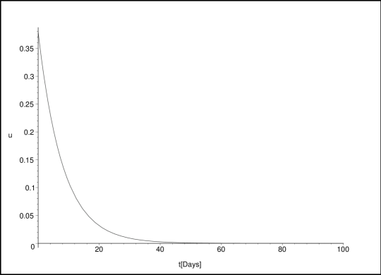
Figure 1: Analytical optimal control $u(t)$ (53) for problem (1)–(7).

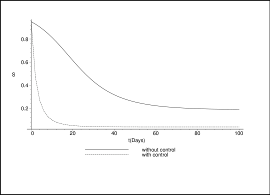
Figure 2: Susceptible individuals $S(t)$ in case of optimal control (53) versus without control.

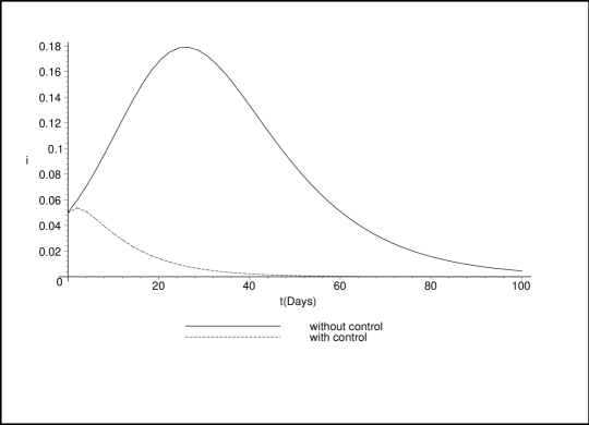
Figure 3: Infected individuals $I(t)$ in case of optimal control (53) versus without control.

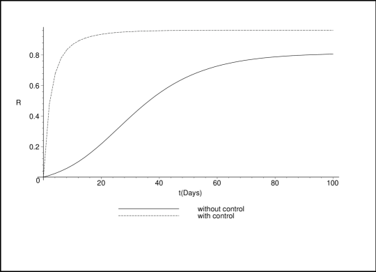
Figure 4: Removed individuals $R(t)$ in case of optimal control (53) versus without control.

5 Conclusions

The analytical expression (53) for the optimal control drawn at Figure 1 is very similar to the optimal control numerically depicted in [6]. Similarly, Figures 2, 3 and 4, respectively for the susceptible, infected and removed individuals, are identical to the corresponding numerical results of [6]. We conclude that the numerical solutions found in [6] provide a good approximation to our analytical expressions.

We claim that the analytical method proposed here can also be applied with success to other problems of optimal control in mathematical epidemiology such as vector-borne, air-borne and water-borne diseases. This question is under investigation and will be addressed elsewhere.

Appendix A Maple code

We have used the computer algebra system Maple for all the computations. The reader interested in this computer algebra system is referred, e.g., to [4].

A.1 Maple code for Example 1

> restart:
> with(Physics):
> eq10:=J=Intc(diff(u(tau),tau)^(2)+1/2*A*u(tau)^2, tau);
> eq20:=Fundiff(eq10,u(t));
> eq20A:=dsolve({eq20,u(0)=U[0]});
> eq20B:=subs(_C2=U[0],eq20A);
> nas:=diff(S(t),t)=-beta*S(t)*i(t);
> nasB:=diff(i(t),t)=beta*S(t)*i(t)-u(t)*i(t);
> eq:=diff(i(t),t)=beta*S[0]*i(t)-rhs(eq20B)*i(t);
> eq1:=simplify(dsolve({eq,i(0)=iota[0]}),power,symbolic);
> eq2:=simplify(int(convert(series(rhs(eq1),t=0,2),polynom),t=0..T)
       + int((rhs(eq20B))^2*A/2,t=0..T),power,symbolic);
> eq3:=simplify(isolate(diff(eq2,U[0])=0,U[0]));

A.2 Maple code for the Ebola optimal control problem (1)–(7)

> restart:
> with(Physics):
> eq1:=J=Intc(diff(u(tau),tau)^(2)+1/2*A*u(tau)^2, tau);
> J(u) = Int([diff(u(tau),tau)^2+1/2*A*u(tau)^2],tau = 0 .. T);
> nis:=K(U[0])=Int(G(tau,A,U[0],Y[0]),tau=0..T)
         +(A/2)*int((U[0]*exp(-1/2*2^(1/2)*A^(1/2)*tau))^2,tau=0..T);
> nas:=diff(rhs(nis),U[0])=0;
> eq2:=Fundiff(eq1,u(t));
> eq4:=subs(_C2=U[0],dsolve({eq2,u(0)=U[0]}));
> restart:
> auxi:=u(t) = U[0]*exp(-1/2*2^(1/2)*A^(1/2)*t);
> aux0:=diff(s(t),t)=-rhs(auxi)*s(t);
> aux0A:=simplify(dsolve({aux0,s(0)=S[0]}),power,symbolic);
> aux0B:=s(t)=convert(series(rhs(aux0A),t=0,3),polynom);
> aux:=diff(i(t),t)=beta*s(t)*i(t)-mu*i(t);
> auxA:=subs(aux0A,aux);
> aux1:=dsolve({auxA,i(0)=iota[0]});
> aux1A:=i(t)=simplify(convert(series(rhs(aux1),t=0,5),polynom),power,symbolic);
> aux1B:=int(rhs(aux1A),t=0..T)+int(A*(rhs(auxi))^2/2,t=0..T);
> plas:=K(U[0])=subs(iota[0]=i[0],aux1B);
> plas1:=K(U[0])=i[0]*T+E[2]*T^2+E[3]*T^3
             +i[0]/48*E[4]*T^4-i[0]/240*E[5]*T^5
             +1/4*U[0]^2*2^(1/2)*A^(1/2)
             -1/4*2^(1/2)*A^(1/2)*U[0]^2*exp(-2^(1/2)*A^(1/2)*T);
> aux1C:=diff(aux1B,U[0])=0;
> aux1D:=isolate(aux1C,U[0]);
> yiyi:=U[0]*exp(-1/2*2^(1/2)*A^(1/2)*T/2)=U[0]/Q;
> isolate(U[0]*exp(-1/2*2^(1/2)*A^(1/2)*T/2)=U[0]/Q,A);
> param:={mu=0.1,beta=0.2,iota[0]=0.05,S[0]=0.95,T=100,Q=500};
> solu:=evalf(subs(param,aux1D));
> plot(rhs(solu),A=0.001..0.1);
> solu1:=evalf(isolate(U[0]*exp(-1/2*2^(1/2)*A^(1/2)*100/2)=U[0]/500,A));
> solu2:=evalf(subs(solu1,solu));
> plot(subs(solu2,solu1,rhs(auxi)),t=0..100);
> u:=subs(solu2,solu1,rhs(auxi));
> plot(u,t=0..100);
> with(plots):
> beta:=0.2;
> mu:=0.1;
> sysnc := diff(s(t),t)=-beta*s(t)*i(t),diff(i(t),t)=beta*s(t)*i(t)-mu*i(t),
                diff(r(t),t)=mu*i(t):
> fcns := {s(t),i(t),r(t)}:
> p:= dsolve({sysnc,s(0)=0.95,i(0)=0.05,r(0)=0},fcns,type=numeric,method=classical):
> odeplot(p, [[t,s(t)],[t,i(t)],[t,r(t)]],0..100);
> g:=odeplot(p, [[t,r(t)]],0..100,color=blue):
> gA:=odeplot(p, [[t,s(t)]],0..100,color=blue):
> gB:=odeplot(p, [[t,i(t)]],0..100,color=blue):
> sysc := diff(s(t),t)=-beta*s(t)*i(t)-u*s(t),
              diff(i(t),t)=beta*s(t)*i(t)-mu*i(t),
              diff(r(t),t)=mu*i(t)+u*s(t):
> fcns := {s(t),i(t),r(t)}:
> pc:= dsolve({sysc,s(0)=0.95,i(0)=0.05,r(0)=0},fcns,type=numeric,method=classical):
> sysc;
> odeplot(pc, [[t,s(t)],[t,i(t)],[t,r(t)]],0..50);
> g1:=odeplot(pc, [[t,r(t)]],0..100,color=red):
> g1A:=odeplot(pc, [[t,s(t)]],0..100,color=red):
> g1B:=odeplot(pc, [[t,i(t)]],0..100,color=red):
> display(g,g1);
> display(gA,g1A);
> display(gB,g1B);

References

- [1] A. Atangana and E. F. Doungmo Goufo, On the Mathematical Analysis of Ebola Hemorrhagic Fever: Deathly Infection Disease in West African Countries, BioMed Research International (2014), Art. ID 261383, 7 pp.
- [2] M. Levi, Classical mechanics with calculus of variations and optimal control, Student Mathematical Library, 69, Amer. Math. Soc., Providence, RI, 2014.
- [3] J. A. Lewnard, M. L. Ndeffo Mbah, J. A. Alfaro-Murillo, F. L. Altice, L. Bawo, T. G. Nyenswah and A. P. Galvani, Dynamics and control of Ebola virus transmission in Montserrado, Liberia: a mathematical modelling analysis, The Lancet 14 (2014), no. 12, 1189–1195.
- [4] S. Lynch, Dynamical systems with applications using MapleTM, second edition, Birkhäuser Boston, Boston, MA, 2010.
- [5] A. Marzi and D. Falzarano, An updated Ebola vaccine: immunogenic, but will it protect?, The Lancet 385 (2015), no. 9984, 2229–2230.
- [6] A. Rachah and D. F. M. Torres, Mathematical Modelling, Simulation, and Optimal Control of the 2014 Ebola Outbreak in West Africa, Discrete Dyn. Nat. Soc. (2015), Art. ID 842792, 9 pp. arXiv:1503.07396
- [7] A. Rachah and D. F. M. Torres, Modelling and Numerical Simulation of the Recent Outbreak of Ebola. In: Proceedings of the 2nd International Conference on Numerical and Symbolic Computation: Developments and Applications (SYMCOMP 2015), Universidade do Algarve, Faro, March 26-27, 2015. Edited by APMTAC (Editors: A. Loja, J. I. Barbosa and J. A. Rodrigues), 179–190.
- [8] X.-S. Wang and L. Zhong, Ebola outbreak in West Africa: real-time estimation and multiple-wave prediction, Math. Biosci. Eng. 12 (2015), no. 5, 1055–1063.