The ${\cal Q}$-cut Representation of One-loop Integrands and Unitarity Cut Method

Abstract

Recently, a new construction for complete loop integrands of massless field theories has been proposed, with on-shell tree-level amplitudes delicately incorporated into its algorithm. This new approach reinterprets integrands in a novel form, namely the $\mathcal{Q}$-cut representation. In this paper, by deriving one-loop integrands as examples, we elaborate in details the technique of this new representation, e.g., the summation over all possible $\mathcal{Q}$-cuts as well as helicity states for the non-scalar internal particle in the loop. Moreover, we show that the integrand in the ${\cal Q}$-cut representation naturally reduces to the integrand in the traditional unitarity cut method for each given cut channel, providing a cross-check for the new approach.

1 Introduction

The attempt to calculate scattering amplitudes at tree and loop-levels over the past decade (see reviews, e.g., Bern:2007dw ; Elvang:2013cua ; Henn:2014yza ) has revealed the great computational ability of on-shell methods. For example, the recursive method, such as the BCFW recursion relation Britto:2004ap ; Britto:2005fq , enables one to build all $n$-point tree-level amplitudes purely through the simplest on-shell objects, e.g., the 3-point tree amplitudes, for a broad range of field theories. Another powerful on-shell technique is the unitarity cut Bern:1994zx ; Bern:1994cg (with its generalization to $D$-dimension Anastasiou:2006jv ; Anastasiou:2006gt ), or the generalized unitarity method Britto:2004nc ; Britto:2005ha which attacks amplitudes at loop-level. Combined with the reduction methods (for example, the computational algebraic geometry methods Zhang:2012ce ; Mastrolia:2012an ), it greatly simplifies the construction of multi-loop amplitudes, through lower-loop ones or even solely tree amplitudes.

The success of these on-shell methods, especially the BCFW recursion relation at tree-level, inspires people to search for an on-shell construction for loop amplitudes CaronHuot:2010zt ; ArkaniHamed:2010kv ; Boels:2010nw . However, for the latter there are more subtle issues. First of all, when talking about loop amplitudes, we should clarify two terminologies, namely the loop integrand and the loop integral after integration. Due to the fact that, the integrand is a rational function of loop as well as external momenta, whose analytic behavior is very similar to tree amplitudes, it is natural to expect a similar recursion relation for it. Although such intuition is correct, the rational function at loop-level possesses two major differences, compared to that of tree-level, which might greatly obstruct the construction of loop integrands. The first difference is the ambiguity of how to define the loop momentum. Under proper regularizations tHooft:1972fi ; Collins:1986 ; Bern:1991aq (such as the dimensional regularization), we can arbitrarily shift the loop momentum while keeping its integration invariant. Because of this degree of freedom, in general it is difficult to identify a unique definition simultaneously for all Feynman diagrams (the planar diagram is an exception, where a canonical ordering of loop momenta do exist thanks to color ordering ArkaniHamed:2010kv ). The second crucial difference is the so-called forward limit. When reducing $n$-point $L$-loop Feynman diagrams to $(n+2)$-point $(L-1)$-loop ones by setting an internal propagator on-shell , we do not get the complete set of $(n+2)$-point $(L-1)$-loop Feynman diagrams, since those ones containing forward singularities have been automatically excluded. Thus, when constructing $L$-loop integrands recursively from the complete $(L-1)$-loop integrands, we should manually exclude those singular parts, and this is not an easy task. Fortunately for some theories, the forward singularities do not exist. One nice example is the planar $\mathcal{N}=4$ super-Yang-Mills (SYM) theory, for which the all-loop recursion relation has been written down, thanks to the absence of two difficulties mentioned above ArkaniHamed:2010kv .

When considering generic theories, the two difficulties mentioned above are inevitable, thus a new idea to handle them is in demand. Quite recently, the authors of ref. Baadsgaard:2015twa provided a new algorithm, namely the $\mathcal{Q}$-cut construction, which delicately resolves these issues. This algorithm derives an expression (namely the $\mathcal{Q}$-cut representation) of loop integrands which looks quite different from the familiar one generated from Feynman diagrams. Here, a canonical way of defining loop momenta can be prescribed, regardless of the loop amplitude considered is color-ordered or not. Also, with a certain kind of scale deformation, the forward singularities can be neatly stripped off.

Although the general framework of $\mathcal{Q}$-cut construction has been settled in Baadsgaard:2015twa , in order to completely understand its structure, further demonstrations in details are still needed. For instance, when summing over all possible $\mathcal{Q}$-cut terms, what rules shall we follow to avoid over-counting or missing some terms? Furthermore, if the internal particle of the loop is not scalar but fermion or gluon, how shall we sum over the helicity states? Besides, the divergence after the loop integration demands us to properly regularize it. Since the most common regularization scheme is the dimensional regularization, we would like to see how ${\cal Q}$-cut construction fits itself into this scheme. Addressing these points with ample examples of one-loop amplitudes would be our first pursuit in this paper.

We want to emphasize that, the ${\cal Q}$-cut construction is a complete algorithm. It gives the construction of loop integrands in ${\cal Q}$-cut representation and the correct physical contours to do the loop integrations Baadsgaard:2015twa . However, since the ${\cal Q}$-cut representation is very different from the familiar integrand generated by Feynman diagrams with quadratic propagators, it would be illustrative to perform a cross-check by using another completely independent algorithm. Our second pursuit here is to provide such a cross-check via the unitarity cut method. We will show that, for each unitarity cut of a given one-loop amplitude, the contribution from ${\cal Q}$-cut representation is identical to the product of two on-shell tree amplitudes under the traditional unitarity cut, thus verifying the equivalence between these two algorithms.

This paper is organized as follows. In §2, we will review the $\mathcal{Q}$-cut representation and unitarity cut method, and discuss the connection between them. In §3 and §4, we use various examples of one-loop amplitudes in scalar field and Yang-Mills theories to demonstrate the details of $\mathcal{Q}$-cut representation, and perform a cross-check by the unitarity cut. The conclusion and discussions are given in §5, and in the appendix, conventions for helicity choice of gluon in $D$-dimension as well as all $D$-dimensional 4-point tree amplitudes are given.

2 Review and general discussions

In this section, we will firstly review the new $\mathcal{Q}$-cut construction of loop integrands proposed in Baadsgaard:2015twa . Since its result is quite different from the one given by standard Feynman diagrams (where the propagators are quadratic), understanding this new structure from various aspects would be of interest. As mentioned in the introduction, we will provide such an digestion based on the unitarity cut method. So the relevant background of unitarity cut will be reviewed shortly afterwards. Then we will present the general aspects of how these two different algorithms are connected.

2.1 Construction of the ${\cal Q}$-cut representation

The working experience of on-shell recursion relations at tree-level tells us that, a nice way of determining a rational function is to apply the residue theorem by some proper deformation. For tree amplitudes, the BCFW deformation is the simplest choice involving minimal number of external legs, while maintaining the on-shell condition and momentum conservation. For loop integrands, similar attempt is not successful due to the two difficulties mentioned before. However, the ambiguity of defining the loop momentum, on the other hand, also allows us to shift its components. Thinking it further, to avoid its entanglement with external momenta, we could shift its components in extra dimensions. For loop momenta, this operation is feasible, since in the dimensional regularization scheme, although all external momenta are kept in 4-dimension, we do need to take loop momenta into $(4-2\epsilon)$-dimension, i.e., $\widetilde{\ell}_{4-2\epsilon}=(\ell_{{\tiny\mbox{4-dim}}},\vec{\mu}_{-2\epsilon})$. With this observation, we can shift the loop momentum as $\widetilde{\ell}\to\widetilde{\ell}+\vec{\eta}$. So the internal propagators are deformed as $(\widetilde{\ell}+P)^{2}\to(\widetilde{\ell}+P)^{2}+z$ ($z=\vec{\eta}^{2}$) with arbitrary 4-dimensional momentum $P$, provided $\widetilde{\ell}\cdot\vec{\eta}=0$. Such a shift can be achieved by either shifting $\vec{\eta}$ in extra dimensions (so $\widetilde{\ell}_{4-2\epsilon}\to(\widetilde{\ell}_{4-2\epsilon},\vec{\eta})$), or keeping $\vec{\eta}$ in the $(-2\epsilon)$-dimension (so $\widetilde{\ell}_{4-2\epsilon}\to(\ell_{{\tiny\mbox{4-dim}}},\vec{\mu}+\vec{\eta})$) with additional condition $\vec{\mu}\cdot\vec{\eta}=0$. No matter which way is taken, the shift is always performed in extra dimensions. Thus we may call it the dimensional deformation. To avoid confusion, hereafter we will use $\widetilde{\ell}$ to denote the loop momentum in $(4-2\epsilon)$-dimension and $\ell$ the 4-dimensional component, i.e., $\widetilde{\ell}=(\ell,\vec{\mu})$. Moreover, we will use $\widehat{\ell}=\widetilde{\ell}+\vec{\eta}$ to denote the deformed loop momentum.

Then, we can continue to discuss the rational function ${\cal I}(\widetilde{\ell})$ obtained from Feynman diagrams, and consider the familiar contour integration $\oint{dz\over z}{\cal I}(\widehat{\ell})$. Unlike the tree amplitude, for this case it is easy to check that its boundary contribution (i.e., the residue at $z=\infty$) is a scale-free rational function in terms of $\widetilde{\ell}$. Thus it integrates to zero under dimensional regularization and hence can be dropped. The residues of finite poles take the form

$${1\over(\widetilde{\ell}+P_{0})^{2}}\left\{{{\cal N}(\widehat{\ell})\over\prod(\widehat{\ell}+P_{i})^{2}}\right\}_{(\widehat{\ell}+P_{0})^{2}=0}~{},$$

where the condition $(\widehat{\ell}+P_{0})^{2}=0$ means nothing but putting this internal propagator on-shell (in higher dimension). More specifically, while ${1\over(\widetilde{\ell}+P_{0})^{2}}$ is an off-shell internal propagator, the expression inside the bracket is an on-shell tree amplitude. Such a form has exactly the same structure as the tree-level BCFW formula ${1\over P^{2}}\left\{A_{L}(\widehat{P})A_{R}(-\widehat{P})\right\}$. Once the residues of all finite poles are obtained, we can perform a further shift term-by-term by translating $\widetilde{\ell}+P_{0}\to\widetilde{\ell}$, such that each off-shell propagator ${1\over(\widetilde{\ell}+P_{0})^{2}}$ is replaced by ${1\over\widetilde{\ell}^{2}}$. The legal shift of loop momenta under proper regularization will not alter the final result after integration, and this kind of shift leads us to the canonical definition of loop momentum.

Next, we need to impose on-shell conditions for the expression inside the bracket. This is achieved by rewriting quadratic propagator $(\widehat{\ell}+P)^{2}$ as a linear propagator $(2\widetilde{\ell}\cdot P+P^{2})$. More specifically, under the dimensional deformation, we will arrive at expressions like

$${\cal I}^{\cal Q}_{{\tiny\mbox{step-1}}}(\widetilde{\ell})=\sum{1\over\widetilde{\ell}^{2}}\left[{{\cal N}(\widetilde{\ell})\over\prod(2\widetilde{\ell}\cdot P_{i}+P_{i}^{2})}\right]~{}.~{}~{}~{}$$ (1)

As emphasized in ref. Baadsgaard:2015twa , the forward limit singularities prevent us from interpreting ${\cal I}^{\cal Q}_{{\tiny\mbox{step-1}}}$ as the full on-shell tree amplitudes. In order to obtain a well-defined result, we need to take a second deformation, namely the scale deformation $\widetilde{\ell}\to{\alpha}\widetilde{\ell}$ and then evaluate the contour integration $\oint{d{\alpha}\over({\alpha}-1)}{\cal I}^{\cal Q}_{{\tiny\mbox{step-1}}}({\alpha}\widetilde{\ell})$. After dropping the residues of poles at ${\alpha}=0$ and ${\alpha}=\infty$, which are scale-free terms so they integrate to zero, we finally arrive at the ${\cal Q}$-cut representation of the loop integrand,

$${\cal I}_{n}^{\cal Q}(\ell)=\sum_{P_{L}}\sum_{h_{1},h_{2}}{\cal A}_{L}(\cdots,\widehat{\ell}_{R}^{~{}h_{1}},-\widehat{\ell}_{L}^{~{}h_{2}}){1\over\widetilde{\ell}^{2}}{1\over(-2\widetilde{\ell}\cdot P_{L}+P_{L}^{2})}{\cal A}_{R}(\widehat{\ell}_{L}^{~{}\bar{h}_{2}},-\widehat{\ell}_{R}^{~{}\bar{h}_{1}},\cdots)~{},~{}~{}~{}$$ (2)

where $\widehat{\ell}_{L}=\alpha_{L}(\widetilde{\ell}+\vec{\eta})$, $\widehat{\ell}_{R}\equiv\widehat{\ell}_{L}-P_{L}$ with $\alpha_{L}=P_{L}^{2}/(2\widetilde{\ell}\cdot P_{L})\neq 0$ and $\vec{\eta}^{2}=\widetilde{\ell}^{2}$ (see Figure (1.a)).

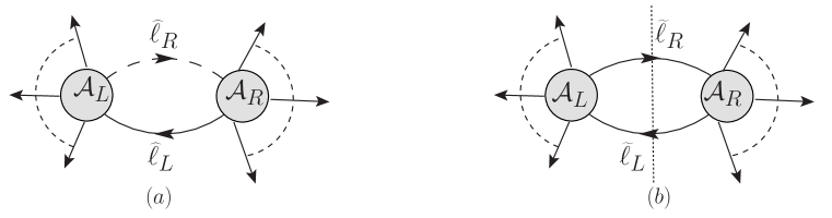
Figure 1: (a) Graphic presentation of ${\cal Q}$-cut: the tree amplitudes are evaluated with the rescaled $D$-dimensional loop momenta $\widehat{\ell}_{L}$ and $\widehat{\ell}_{R}$, multiplied by two novel propagators $1/\ell^{2}$ and $1/(2\ell\cdot P_{L}+P_{L}^{2})$. (b) Graphic presentation of unitarity cut: the tree amplitudes are evaluated with the on-shell loop momenta $\widetilde{\ell}_{L}$ and $\widetilde{\ell}_{R}$, with two propagators $1/\widetilde{\ell}_{L}^{2}\widetilde{\ell}_{R}^{2}$ replaced by $\delta^{+}(\widetilde{\ell}_{L}^{2})\delta^{+}(\widetilde{\ell}_{R}^{2})$.

Let us explain more details of the ${\cal Q}$-cut representation (2). Firstly, although $\vec{\eta}$ does appear in $\widehat{\ell}_{L}$, it should be eliminated together with ${\cal A}_{L},{\cal A}_{R}$ by the on-shell condition $\vec{\eta}^{2}=\widetilde{\ell}^{2}$. After that, all propagators involving $\widehat{\ell}$ become linear in $\widetilde{\ell}$. Secondly, since in this algorithm two different deformations have been performed and each one sets an internal propagator on-shell, these two on-shell propagators are not equivalent. This is entirely different from unitarity cut where the two cut propagators are essentially equivalent. Due to this difference, the sum over $P_{L}$ (with condition $P_{L}^{2}\neq 0$) includes all possible partitions of external legs associated with ${\cal Q}$-cut, without modulo the cyclic group. Thus, as we will see soon, two terms in ${\cal Q}$-cut representation of momenta $P_{L}$ and $-P_{L}$ correspond to a single unitarity cut of momentum $P_{L}$.

Now we move to the second summation in (2), which should be carefully treated when the internal particle along $\ell_{L}$ or $\ell_{R}$ is not a scalar. As emphasized before, in the ${\cal Q}$-cut construction, we have met three different kind of dimensions: the plain 4-dimension for external momenta, the $(4-2\epsilon)$-dimension for loop momenta under the dimensional regularization, and the $(4-2\epsilon+d)$-dimension for the deformed loop momenta. A question naturally arises: when we sum over helicity states of internal particles, which dimension should we use, the $(4-2\epsilon)$-dimension or the $(4-2\epsilon+d)$-dimension? The correct treatment is to sum over helicity states in the $(4-2\epsilon)$-dimension. This can be explained via the following two arguments. Firstly, according to the Feynman rules in dimensional regularization, before setting the internal propagator on-shell, the metric $\eta_{\mu\nu}$ we use is of $(4-2\epsilon)$-dimension. Secondly, as explained before, the dimensional deformation can be also interpreted as deforming $\vec{\mu}\to\vec{\mu}+\vec{\eta}$ in the $(-2\epsilon)$-dimension with additional condition $\vec{\mu}\cdot\vec{\eta}=0$, in which case we have not defined the $(4-2\epsilon+d)$-dimension at all.

Before concluding this part, we will give a brief remark. While enjoying all advantages of on-shell tree amplitudes as building blocks, the ${\cal Q}$-cut representation systematically produces a completely off-shell one-loop integrand. This is different from the traditional unitarity cut method, where after getting all pieces of integrand for each unitarity cut, we should assemble them carefully to produce the full integrand, avoiding over-counting or missing terms. The only price (or novelty) of these accomplishments in the new approach is to replace the quadratic propagators by rescaled linear propagators.

2.2 Unitarity cut method

The Passarino-Veltman reduction Passarino:1978jh is a standard method of computing loop amplitudes. In its context, an one-loop amplitude ${\cal A}$ of massless theories can be expanded as some master integrals Bern:1992em ; Bern:1993kr as ${\cal A}=\sum_{i}c_{i}\int d^{4-2\epsilon}\ell~{}{\cal I}_{i}$, where $c_{i}$ is an expansion coefficient (a rational function of external kinematic data) and ${\cal I}_{i}$ is a scalar integrand of pentagon, box, triangle and bubble topologies. Thus the computation of generic one-loop amplitudes can be reduced to determining of coefficients $c_{i}$, while the unitarity cut method is good for this purpose Anastasiou:2006jv ; Anastasiou:2006gt ; Britto:2004nc ; Britto:2005ha ; Britto:2006sj ; Ossola:2006us ; Britto:2006fc ; Britto:2007tt ; Forde:2007mi ; Ellis:2007br ; Giele:2008ve ; Ossola:2008xq ; Badger:2008cm .

More explicitly, for the unitarity cut in $s_{P}$ channel with respect to the cut momentum $P$, as shown in Figure (1.b), we evaluate

$$\Delta{\cal A}^{\tiny\mbox{1-loop}}_{n}(\widetilde{\ell})|_{P}=\int d\Omega~{}{\cal I}^{\tiny\mbox{1-loop}}_{n}(\widetilde{\ell})|_{P}~{},~{}~{}~{}$$ (3)

where ${\cal I}^{\tiny\mbox{1-loop}}_{n}(\widetilde{\ell})|_{P}\equiv{\cal I}~{}\widetilde{\ell}_{L}^{2}~{}\widetilde{\ell}_{R}^{2}$ is the cut integrand obtained via multiplying the full one-loop integrand by two cut propagators $\widetilde{\ell}_{L}^{2},\widetilde{\ell}_{R}^{2}$. The integration measure above is given by

$$\int d\Omega=\int d^{\dim[\widetilde{\ell}]}\widetilde{\ell}_{L}~{}d^{\dim[\widetilde{\ell}]}\widetilde{\ell}_{R}~{}\delta^{+}(\widetilde{\ell}_{L}^{~{}2})\delta^{+}(\widetilde{\ell}_{R}^{~{}2})\delta^{\dim[\widetilde{\ell}]}(\widetilde{\ell}_{R}-\widetilde{\ell}_{L}+P)~{}.~{}~{}~{}$$ (4)

Here, $\Delta{\cal A}^{\tiny\mbox{1-loop}}_{n}(\widetilde{\ell})|_{P}$ is the imaginary part with respect to $P$. It is also crucial to note that in unitarity cut, cut momentum $P$ is equivalent to $-P$, since it just corresponds to $\widetilde{\ell}_{R}\leftrightarrow\widetilde{\ell}_{L}$. Thus when talking about all possible cuts, we should in fact consider all inequivalent $\{P,-P\}$ pairs.

The unitarity cut can be applied to the one-loop amplitude reduction. Since $c_{i}$ has no branch cut, we have $\Delta{\cal A}=\sum_{i}c_{i}\Delta\int d^{4-2\epsilon}\widetilde{\ell}~{}{\cal I}_{i}$. Furthermore, for different master integrals, $\Delta\int d^{4-2\epsilon}\widetilde{\ell}~{}{\cal I}_{i}$ are distinct analytic functions. Thus by comparing both sides of the expansion, we can determine coefficients $c_{i}$.

The central idea of the unitarity cut method relies on the fact that, the cut integrand ${\cal I}^{\tiny\mbox{1-loop}}_{n}(\widetilde{\ell})|_{P}$ is given by

$${\cal I}^{\tiny\mbox{1-loop}}_{n}(\widetilde{\ell})|_{P}=\sum_{h_{1},h_{2}}{\cal A}_{L}(\cdots,\widetilde{\ell}_{R}^{~{}h_{1}},-\widetilde{\ell}_{L}^{~{}h_{2}}){\cal A}_{R}(\widetilde{\ell}_{L}^{~{}\bar{h}_{2}},-\widetilde{\ell}_{R}^{~{}\bar{h}_{1}},\cdots)~{}.~{}~{}~{}$$ (5)

Thus when computing the expansion coefficients, we do not have to start with the full one-loop integrand, which is usually given by Feynman diagrams. Since the on-shell tree amplitudes are much simpler to compute, the unitarity cut indeed greatly improves the efficiency of loop amplitude computation.

2.3 Connection between two approaches

Having reviewed the ${\cal Q}$-cut construction and the unitarity cut method, let us move to one of our major concerns, i.e., understanding the ${\cal Q}$-cut construction. Since this is a complete approach, we should have

$$\int d^{\dim[\widetilde{\ell}]}\widetilde{\ell}~{}{\cal I}^{\cal Q}(\widetilde{\ell})=\int d^{\dim[\widetilde{\ell}]}\widetilde{\ell}~{}{\cal I}^{\cal F}(\widetilde{\ell})~{},~{}~{}~{}$$ (6)

where ${\cal I}^{\cal Q}$ and ${\cal I}^{\cal F}$ are loop integrands produced by ${\cal Q}$-cut construction and Feynman diagrams respectively. For generic theories, the loop integrand of course will be very complicated and these two integrands would look quite different. Thus their direct comparison is practically impossible for most of cases, let alone further integrating them out. However, as we have mentioned, the calculation of one-loop amplitudes is equivalent to fixing all coefficients $c_{i}$ of master integrals. If we can show that, the same coefficients can be obtained by using ${\cal I}^{\cal Q}(\widetilde{\ell})$ as the input for (3), the identity (6) must hold.

Let us consider the following expression

$$\int d^{\dim[\widetilde{\ell}]}\widetilde{\ell}_{L}~{}d^{\dim[\widetilde{\ell}]}\widetilde{\ell}_{R}~{}\delta^{+}(\widetilde{\ell}_{L}^{~{}2})\delta^{+}(\widetilde{\ell}_{R}^{~{}2})\delta^{\dim[\widetilde{\ell}]}(\widetilde{\ell}_{R}-\widetilde{\ell}_{L}+P)$$

$$~{}~{}~{}~{}~{}~{}~{}~{}~{}~{}~{}~{}~{}~{}~{}~{}~{}~{}~{}~{}~{}~{}~{}~{}~{}~{}\times\left\{\widetilde{\ell}_{L}^{~{}2}~{}\widetilde{\ell}_{R}^{~{}2}\sum_{P_{L}}\sum_{h_{1},h_{2}}{{\cal A}_{L}(\cdots,\widehat{\ell}_{R}^{~{}h_{1}},-\widehat{\ell}_{L}^{~{}h_{2}}){\cal A}_{R}(\widehat{\ell}_{L}^{~{}\bar{h}_{2}},-\widehat{\ell}_{R}^{~{}\bar{h}_{1}},\cdots)\over\widetilde{\ell}^{2}(-2\widetilde{\ell}\cdot P_{L}+P_{L}^{2})}\right\}~{},~{}~{}~{}$$ (7)

where the explicit expression of ${\cal I}^{\cal Q}(\widetilde{\ell})$ in (2) has been inserted. In the traditional Feynman diagram approach, it is simple to identify $\widetilde{\ell}_{L}$ and $\widetilde{\ell}_{R}$ with the corresponding propagators in ${\cal I}^{\cal F}(\widetilde{\ell})$. However, in the ${\cal Q}$-cut representation, under the canonical definition of loop momentum for each $\mathcal{Q}$-cut term, there is one and only one quadratic propagator in ${\cal I}^{\cal Q}(\widetilde{\ell})$. Hence two possible identifications are allowed, one is $\widetilde{\ell}=\widetilde{\ell}_{L}$ and the other $\widetilde{\ell}=\widetilde{\ell}_{R}$. Thanks to the factor $\delta^{+}(\widetilde{\ell}_{L}^{2})\delta^{+}(\widetilde{\ell}_{R}^{2})\widetilde{\ell}_{L}^{2}~{}\widetilde{\ell}_{R}^{2}$, it is easy to see that when taking $\widetilde{\ell}=\widetilde{\ell}_{L}$, the only surviving term is the one with $P_{L}=P$, and expression (7) reduces to

$$\int d^{\dim[\widetilde{\ell}]}\widetilde{\ell}_{L}~{}d^{\dim[\widetilde{\ell}]}\widetilde{\ell}_{R}~{}\delta^{+}(\widetilde{\ell}_{L}^{~{}2})\delta^{+}(\widetilde{\ell}_{R}^{~{}2})\delta^{\dim[\widetilde{\ell}]}(\widetilde{\ell}_{R}-\widetilde{\ell}_{L}+P)\sum_{h_{1},h_{2}}{\cal A}_{L}(\cdots,\widehat{\ell}_{R}^{~{}h_{1}},-\widehat{\ell}_{L}^{~{}h_{2}}){\cal A}_{R}(\widehat{\ell}_{L}^{~{}\bar{h}_{2}},-\widehat{\ell}_{R}^{~{}\bar{h}_{1}},\cdots)~{}.~{}~{}~{}$$ (8)

Recalling $\widehat{\ell}_{L}=\alpha_{L}(\widetilde{\ell}+\vec{\eta})$, $\widehat{\ell}_{R}\equiv\widehat{\ell}-P_{L}$ with $\alpha_{L}=P_{L}^{2}/(2\widetilde{\ell}\cdot P_{L})\neq 0$ and $\vec{\eta}^{2}=\widetilde{\ell}^{2}$, by using $\widetilde{\ell}^{2}=\widetilde{\ell}_{L}^{2}=0$ we obtain $\vec{\eta}=0$. Furthermore, with $\widetilde{\ell}_{R}^{2}=(\widetilde{\ell}-P_{L})^{2}=0$ we obtain $P_{L}^{2}=(2\widetilde{\ell}\cdot P_{L})$, thus ${\alpha}_{L}=1$. Putting all pieces together, we find $\widehat{\ell}_{L}=\widetilde{\ell}_{L}$ and $\widehat{\ell}_{R}=\widetilde{\ell}_{R}$ in the given unitarity cut, then expression (8) reduces to

$$\int d^{\dim[\widetilde{\ell}]}\widetilde{\ell}_{L}~{}d^{\dim[\widetilde{\ell}]}\widetilde{\ell}_{R}~{}\delta^{+}(\widetilde{\ell}_{L}^{~{}2})\delta^{+}(\widetilde{\ell}_{R}^{~{}2})\delta^{\dim[\widetilde{\ell}]}(\widetilde{\ell}_{R}-\widetilde{\ell}_{L}+P)\sum_{h_{1},h_{2}}{\cal A}_{L}(\cdots,\widetilde{\ell}_{R}^{~{}h_{1}},-\widetilde{\ell}_{L}^{~{}h_{2}}){\cal A}_{R}(\widetilde{\ell}_{L}^{~{}\bar{h}_{2}},-\widetilde{\ell}_{R}^{~{}\bar{h}_{1}},\cdots)~{}.~{}~{}~{}$$ (9)

The expression above is exactly the one of (3) with input (5). It tells that, taking ${\cal Q}$-cut representation as the input, we can reproduce the same expansion coefficients $c_{i}$ as those computed by the traditional unitarity cut method.

If we identify $\widetilde{\ell}=\widetilde{\ell}_{R}$, the only surviving term in (7) would be the one with $P_{L}=-P$. After a analogous analysis, it can be checked that now $\widehat{\ell}_{L}=\widetilde{\ell}_{R}$ and $\widehat{\ell}_{R}=\widetilde{\ell}_{L}$. Then (7) reduces to (9) with the relabeling ${\cal A}_{L}\leftrightarrow{\cal A}_{R}$, and it also produces the same expansion coefficients $c_{i}$. In the subsequent part of this paper, we will demonstrate the calculations above with explicit examples.

Now, we give a brief summary of these general arguments. By comparing the expansion coefficients of master integrals produced by the unitarity cut method, we have checked that the ${\cal Q}$-cut representation indeed produces the complete one-loop integrand. Furthermore, we see that while it is non-trivial to assemble the results from all possible unitarity cuts into the full loop integrand with some proper off-shell continuation, the ${\cal Q}$-cut representation provides a more natural solution.

In the following sections, we will go through several examples and clarify the details discussed above.

3 Applications in scalar field theory

The amplitudes of scalar field theory are simple enough to explore the details of $\mathcal{Q}$-cut representation at the level of the full integrand, while the pole structure of non-color-ordered amplitudes resembles that of non-planar amplitudes. Hence it is worthwhile to go through a few examples of both color-ordered and non-color-ordered scalar amplitudes. Since the internal particles of the loop are scalars, in this section, we will use $\ell$ to denote the $(4-2\epsilon)$-dimensional $\widetilde{\ell}$ for simplicity.

3.1 Warmup examples

Before heading to explicit amplitudes, let us start with some warmup exercises, i.e., the scalar integrands of bubble, triangle and box topologies, illustrated in Figure (2). With these examples, we want to clarify the differences between the results of $\mathcal{Q}$-cut construction and the original scalar integrands. These results will be useful for the later discussion of explicit amplitudes.

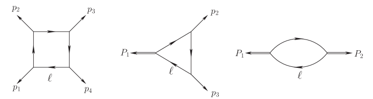
Figure 2: Convention of external momenta for scalar integrands of box, triangle and bubble topologies. $p_{i}$ denotes massless momentum and $P_{i}$ denotes the sum of several massless momenta.

Scalar integrand of bubble topology: Let us focus on the expression

$${\cal I}^{\flat}_{\between}(P_{1};P_{2})={1\over\ell^{2}(\ell-P_{1})^{2}}~{},~{}~{}~{}$$ (10)

where $P_{1}+P_{2}=0$, and $P_{i}$ is the sum of several massless momenta. Applying the general partial fraction identity,

$${1\over D_{1}\cdots D_{m}}=\sum_{i=1}^{m}{1\over D_{i}}\left[\prod_{j\neq i}{1\over D_{j}-D_{i}}\right]~{},~{}~{}~{}$$ (11)

it becomes

$${\cal I}^{\flat}_{\between}(P_{1};P_{2}) = {1\over\ell^{2}((\ell-P_{1})^{2}-\ell^{2})}+{1\over(\ell-P_{1})^{2}(\ell^{2}-(\ell-P_{1})^{2})}~{}.~{}~{}~{}$$ (12)

Since this result should be combined with the loop integration $\int d^{4}\ell$, with proper regularization (such as dimensional regularization), we can shift the loop momentum term-by-term without altering the integrated result. Thus we can write

$${\cal I}^{\flat,pf}_{\between}(P_{1};P_{2})\simeq{1\over\ell^{2}(-2\ell\cdot P_{1}+P_{1}^{2})}+{1\over\ell^{2}(-2\ell\cdot P_{2}+P_{2}^{2})}~{}.~{}~{}~{}$$ (13)

The symbol $\simeq$ means the two expressions are equivalent upon integration. The superscript ^pf denotes the result after partial fraction identity and momentum shifting.

We can also derive the ${\cal Q}$-cut representation of expression (10) by using the two-step deformation reviewed in the previous section. For this simple case, the residues at finite poles of $\alpha$ yields exactly ${\cal I}^{\flat,{\cal Q}}_{\between}(P_{1};P_{2})={\cal I}^{\flat,pf}_{\between}(P_{1};P_{2})$, where the superscript ${\cal Q}$ denotes the result produced by ${\cal Q}$-cut construction. Hence upon integration, we have the following two equivalent expressions

$${1\over\ell^{2}(\ell-P_{1})^{2}}\simeq{1\over\ell^{2}(-2\ell\cdot P_{1}+P_{1}^{2})}+{1\over\ell^{2}(-2\ell\cdot P_{2}+P_{2}^{2})}~{},~{}~{}~{}$$

which can be used in later comparison.

Scalar integrand of triangle topology: Let us focus on the expression

$${\cal I}^{\flat}_{\triangle}(P_{1};p_{2};p_{3})={1\over\ell^{2}(\ell-P_{1})^{2}(\ell+p_{3})^{2}}~{},~{}~{}~{}$$ (14)

where again $P_{1}$ is the sum of several massless momenta. Applying the partial fraction identity (11), and then shifting the loop momentum, we get

$${\cal I}^{\flat,pf}_{\triangle} \simeq {1\over\ell^{2}(-2\ell\cdot P_{1}+P_{1}^{2})(2\ell\cdot p_{3})}+{1\over\ell^{2}(2\ell\cdot P_{1}+P_{1}^{2})(-2\ell\cdot p_{2})}+{1\over\ell^{2}(-2\ell\cdot p_{3})(2\ell\cdot p_{2})}~{}.~{}~{}~{}$$ (15)

The last term is scale-free and can be dropped when performing the loop integration.

Now, we take a second deformation $\ell\to\alpha\ell$ and compute the residues of ${{\cal I}^{\flat,pf}_{\triangle}(\alpha\ell)\over\alpha-1}$ at finite poles of $\alpha$ excluding $\alpha=0,1$. After dropping the scale-free terms, we get

$${\cal I}^{\flat,{\cal Q}}_{\triangle}(P_{1};p_{2};p_{3})={\ell\cdot P_{1}\over\ell^{2}(-2\ell\cdot P_{1}+P_{1}^{2})P_{1}^{2}(\ell\cdot p_{3})}-{\ell\cdot p_{23}\over\ell^{2}(-2\ell\cdot p_{23}+p_{23}^{2})p_{23}^{2}(\ell\cdot p_{2})}~{}.~{}~{}~{}$$ (16)

Unlike the bubble case, it is obvious that ${\cal I}^{\flat,{\cal Q}}_{\triangle}(P_{1};p_{2};p_{3})\neq{\cal I}^{\flat,pf}_{\triangle}(P_{1};p_{2};p_{3})$. Nonetheless, it is yet easy to figure out that

$${\cal I}^{\flat,{\cal Q}}_{\triangle}(P_{1};p_{2};p_{3})-{\cal I}^{\flat,pf}_{\triangle}(P_{1};p_{2};p_{3}) \simeq {2\ell\cdot P_{1}-P_{1}^{2}\over\ell^{2}(-2\ell\cdot P_{1}+P_{1}^{2})P_{1}^{2}(2\ell\cdot p_{3})}-{2\ell\cdot p_{23}-p_{23}^{2}\over\ell^{2}(-2\ell\cdot p_{23}+p_{23}^{2})p_{23}^{2}(2\ell\cdot p_{2})}$$ (17)

$$= {-1\over\ell^{2}P_{1}^{2}(2\ell\cdot p_{3})}-{-1\over\ell^{2}p_{23}^{2}(2\ell\cdot p_{2})}\simeq 0~{},~{}~{}~{}$$

where the last line is a scale-free expression which integrates to zero. This is the first non-trivial example showing that, although the ${\cal Q}$-cut representation of a loop integrand is different from the one given by Feynman diagrams, their integrated results still match. Hence upon integration, we have the following two equivalent expressions

$${1\over\ell^{2}(\ell-P_{1})^{2}(\ell+p_{3})^{2}}\simeq{\ell\cdot P_{1}\over\ell^{2}(-2\ell\cdot P_{1}+P_{1}^{2})P_{1}^{2}(\ell\cdot p_{3})}-{\ell\cdot p_{23}\over\ell^{2}(-2\ell\cdot p_{23}+p_{23}^{2})p_{23}^{2}(\ell\cdot p_{2})}~{},~{}~{}~{}$$

which can be used in later comparison.

Scalar integrand of box topology: Let us focus on the expression

$${\cal I}^{\flat}_{\Box}(p_{1};p_{2};p_{3};p_{4})={1\over\ell^{2}(\ell-p_{1})^{2}(\ell-p_{12})^{2}(\ell+p_{4})^{2}}~{}.~{}~{}~{}$$ (18)

Applying the partial fraction identity (11) and shifting the loop momentum, we get

$${\cal I}_{\Box}^{\flat,pf} \simeq {1\over\ell^{2}}\Big{(}{1\over(-2\ell\cdot p_{1})(-2\ell\cdot p_{12}+p_{12}^{2})(2\ell\cdot p_{4})}+{1\over(2\ell\cdot p_{1})(-2\ell\cdot p_{2})(2\ell\cdot p_{41}+p_{41}^{2})}$$ (19)

$$~{}~{}~{}~{}~{}~{}~{}~{}~{}~{}+{1\over(2\ell\cdot p_{12}+p_{12}^{2})(2\ell\cdot p_{2})(-2\ell\cdot p_{3})}+{1\over(-2\ell\cdot p_{4})(-2\ell\cdot p_{41}+p_{41}^{2})(2\ell\cdot p_{3})}\Big{)}~{}.~{}~{}~{}$$

For this example, we can directly use formula (2) to write the ${\cal Q}$-cut representation of expression (18), which is given by

$${\cal I}^{\flat,{\cal Q}}_{\Box}(p_{1};p_{2};p_{3};p_{4}) \simeq {\ell\cdot p_{12}\over(\ell\cdot p_{1})p_{12}^{2}}{1\over\ell^{2}(-2\ell\cdot p_{12}+p_{12}^{2})}{\ell\cdot p_{34}\over(\ell\cdot p_{4})p_{34}^{2}}+\mbox{Cyclic}\{p_{1},p_{2},p_{3},p_{4}\}~{}.~{}~{}~{}$$ (20)

Again, it is easy to figure out that the difference of (20) and (19) is a scale-free expression. So although the expression ${\cal I}^{\flat,{\cal Q}}_{\Box}(p_{1};p_{2};p_{3};p_{4})$ is apparently different from ${\cal I}^{\flat,pf}_{\Box}(p_{1};p_{2};p_{3};p_{4})$, they are equivalent upon integration. Hence we have the following two equivalent expressions

$${1\over\ell^{2}(\ell-p_{1})^{2}(\ell-p_{12})^{2}(\ell+p_{4})^{2}}\simeq{\ell\cdot p_{12}\over(\ell\cdot p_{1})p_{12}^{2}}{1\over\ell^{2}(-2\ell\cdot p_{12}+p_{12}^{2})}{\ell\cdot p_{34}\over(\ell\cdot p_{4})p_{34}^{2}}+\mbox{Cyclic}\{p_{1},p_{2},p_{3},p_{4}\}~{},~{}~{}~{}$$

which can be used in later comparison.

3.2 Color-ordered 4-point amplitude in $\phi^{4}$ theory

Now, let us consider the one-loop amplitudes in scalar field theory, and the first one is the color-ordered $\phi^{4}$ theory. The analysis will be presented as follows. Firstly we compute the loop integrand by Feynman diagrams, next we compute the loop integrand by $\mathcal{Q}$-cut construction. Then we will compare these two integrands directly and show their equivalence upon loop integration, followed by a discussion in the context of unitarity cut, which provides another independent cross-check for its validity.

By color-ordered Feynman rules, the integrand of the 4-point one-loop amplitude gets contribution from two bubble diagrams, which is

$${\cal I}^{\cal F}(\ell)={1\over\ell^{2}(\ell-p_{12})^{2}}+{1\over\ell^{2}(\ell-p_{41})^{2}}~{},~{}~{}~{}$$ (21)

while using the ${\cal Q}$-cut construction (2), it is given by

$${\cal I}^{\cal Q} = {\cal A}_{L}(1,2,\widehat{\ell}_{R},-\widehat{\ell}_{L}){1\over\ell^{2}(-2\ell\cdot p_{12}+p_{12}^{2})}{\cal A}_{R}(\widehat{\ell}_{L},-\widehat{\ell}_{R},3,4)+\mbox{Cyclic}\{p_{1},p_{2},p_{3},p_{4}\}~{}.~{}~{}~{}$$ (22)

where $\widehat{\ell}=\alpha(\ell+\eta)$ ($\eta$ is determined by $\ell^{2}-\eta^{2}=0$), and $\alpha$ is the pole’s location specific to that cut. Nonetheless, for $\phi^{4}$ theory the 4-point tree amplitude is trivially $1$, i.e., ${\cal A}_{L}={\cal A}_{R}=1$. Thus we get

$${\cal I}^{\cal Q}(\ell)={1\over\ell^{2}(-2\ell\cdot p_{12}+p_{12}^{2})}+{1\over\ell^{2}(-2\ell\cdot p_{23}+p_{23}^{2})}+{1\over\ell^{2}(-2\ell\cdot p_{34}+p_{34}^{2})}+{1\over\ell^{2}(-2\ell\cdot p_{41}+p_{41}^{2})}~{}.~{}~{}~{}$$ (23)

Obtaining (21) and (23), we can directly compare them. Note that each term in (21) is a standard bubble integrand already known in (10), using result (13) it is easy to see that the first term in (21) is equivalent to the sum of the first and third terms in (23), while the second term in (21) is equivalent to the sum of the second and fourth terms in (23). Hence the one-to-one correspondence obviously ensures the equivalence ${\cal I}^{\cal F}={\cal I}^{\cal Q}$.

Now we consider the unitarity cut for $s_{12}$-channel. The traditional unitarity cut method gives

$$\Delta^{\mathcal{F}}_{s_{12}}=\int d^{4}\ell_{L}d^{4}\ell_{R}~{}\delta^{4}(\ell_{R}-\ell_{L}+p_{12})\delta^{+}(\ell_{L}^{2})\delta^{+}(\ell_{R}^{2})\times{\cal A}_{L}(1,2,\ell_{R},-\ell_{L}){\cal A}_{R}(\ell_{L},-\ell_{R},3,4)~{},~{}~{}~{}$$ (24)

while the contribution from the loop integrand of ${\cal Q}$-cut representation is given by

$$\Delta^{\mathcal{Q}}_{s_{12}}=\int d^{4}\ell_{L}d^{4}\ell_{R}~{}\delta^{4}(\ell_{R}-\ell_{L}+p_{12})\delta^{+}(\ell_{L}^{2})\delta^{+}(\ell_{R}^{2})\times{\cal I}^{\cal Q}(\ell)~{}\ell_{L}^{2}\ell_{R}^{2}~{}.~{}~{}~{}$$ (25)

Let us evaluate (24) first. Since the 4-point tree amplitudes are simply $1$, we have ${\cal A}_{L}{\cal A}_{R}=1$. When we integrate over $\ell_{R}$ along with the momentum conservation delta function, $\Delta^{\mathcal{F}}_{s_{12}}$ becomes

$$\Delta^{\mathcal{F}}_{s_{12}}[\ell_{L}]=\int d^{4}\ell_{L}~{}\delta^{+}(\ell_{L}^{2})\delta^{+}((\ell_{L}-p_{12})^{2})~{},~{}~{}~{}$$ (26)

on the other hand, when we integrate over $\ell_{L}$, $\Delta^{\mathcal{F}}_{s_{12}}$ becomes

$$\Delta^{\mathcal{F}}_{s_{12}}[\ell_{R}]=\int d^{4}\ell_{R}~{}\delta^{+}(\ell_{R}^{2})\delta^{+}((\ell_{R}+p_{12})^{2})~{}.~{}~{}~{}$$ (27)

Now we evaluate (25). Identifying $\ell\to\ell_{L}$ and integrate over $\ell_{R}$ against momentum conservation, we get

$$\Delta^{\mathcal{Q}}_{s_{12}}[\ell_{L}]=\int d^{4}\ell_{L}~{}\delta^{+}(\ell_{L}^{2})\delta^{+}((\ell_{L}-p_{12})^{2})\times\ell_{L}^{2}(\ell_{L}-p_{12})^{2}~{}{\cal I}^{\mathcal{Q}}(\ell_{L})~{}.~{}~{}~{}$$ (28)

Due to the remaining two delta functions, we have $\ell_{L}^{2}=0$ as well as $(\ell_{L}-p_{12})^{2}=0\to-2\ell_{L}\cdot p_{12}+p_{12}^{2}=0$. Thus among the four terms of ${\cal I}^{\mathcal{Q}}$ in (23) when multiplied by $\ell_{L}^{2}(\ell_{L}-p_{12})^{2}$, only the first term survives (which equals to 1) and the rest three terms vanish. Hence we have

$$\Delta^{\mathcal{Q}}_{s_{12}}[\ell_{L}]=\int d^{4}\ell_{L}~{}\delta^{+}(\ell_{L}^{2})\delta^{+}((\ell_{L}-p_{12})^{2})~{}.~{}~{}~{}$$ (29)

Similarly, identifying $\ell\to\ell_{R}$ and integrating over $\ell_{L}$ against momentum conservation, we have

$$\Delta^{\mathcal{Q}}_{s_{12}}[\ell_{R}] = \int d^{4}\ell_{R}~{}\delta^{+}(\ell_{R}^{2})\delta^{+}((\ell_{R}+p_{12})^{2})\times\ell_{R}^{2}(\ell_{R}+p_{12})^{2}~{}{\cal I}^{\mathcal{Q}}(\ell_{R})$$ (30)

$$= \int d^{4}\ell_{R}~{}\delta^{+}(\ell_{R}^{2})\delta^{+}((\ell_{R}+p_{12})^{2})~{}.~{}~{}~{}$$

where only the third term in (23) survives, when multiplied by $\ell_{R}^{2}(\ell_{R}+p_{12})^{2}$ upon on-shell conditions $\ell_{R}^{2}=0$, $(\ell_{R}+p_{12})^{2}=0$. The explicit calculation above verifies the equivalence $\Delta^{\mathcal{Q}}_{s_{12}}[\ell_{L}]=\Delta^{\mathcal{F}}_{s_{12}}[\ell_{L}]$ and $\Delta^{\mathcal{Q}}_{s_{12}}[\ell_{R}]=\Delta^{\mathcal{F}}_{s_{12}}[\ell_{R}]$ in the $s_{12}$-channel unitarity cut. This example also clearly demonstrates how the two terms in ${\cal Q}$-cut representation correspond to one standard unitarity cut.

The $s_{14}$-channel unitarity cut has no essential difference with the $s_{12}$-channel, and the equivalence between two loop integrands generated by Feynman diagrams and $\mathcal{Q}$-cut construction is valid for all cut channels.

3.3 Color-ordered 4-point amplitude in $\phi^{3}$ theory

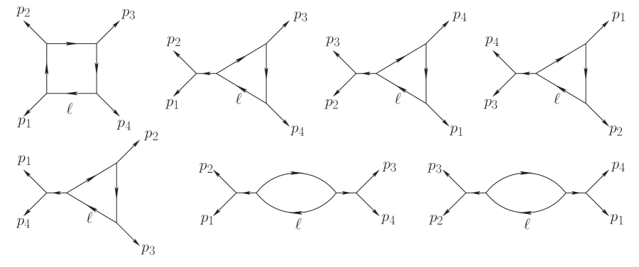
Figure 3: The contributing Feynman diagrams of color-ordered 4-point one-loop amplitude in $\phi^{3}$ theory.

Now we turn to a more complicated example, namely the 4-point one-loop amplitude in $\phi^{3}$ theory.

Directly from Feynman diagrams, the loop integrand is

$${\cal I}^{\cal F} = {\cal I}_{\Box}^{\phi^{3}}+{\cal I}_{\triangle}^{\phi^{3}}+{\cal I}_{\between}^{\phi^{3}}~{},~{}~{}~{}$$ (31)

where

$${\cal I}_{\Box}^{\phi^{3}}={1\over\ell^{2}(\ell-p_{1})^{2}(\ell-p_{12})^{2}(\ell+p_{4})^{2}}~{}~{},~{}~{}{\cal I}_{\triangle}^{\phi^{3}}={1\over\ell^{2}(\ell-p_{12})^{2}(\ell+p_{4})^{2}p_{12}^{2}}+\mbox{Cyclic}\{p_{1},p_{2},p_{3},p_{4}\}~{},$$

$${\cal I}_{\between}^{\phi^{3}}={1\over\ell^{2}(\ell-p_{12})^{2}(p_{12}^{2})^{2}}+{1\over\ell^{2}(\ell-p_{41})^{2}(p_{41}^{2})^{2}}~{}.~{}~{}~{}$$ (32)

Given by ${\cal Q}$-cut construction, the loop integrand is

$${\cal I}^{\mathcal{Q}} = {\cal A}_{L}(1,2,\widehat{\ell}_{R},-\widehat{\ell}_{L}){1\over\ell^{2}(-2\ell\cdot p_{12}+p_{12}^{2})}{\cal A}_{R}(\widehat{\ell}_{L},-\widehat{\ell}_{R},3,4)+\mbox{Cyclic}\{p_{1},p_{2},p_{3},p_{4}\}~{}.~{}~{}~{}$$ (33)

where

$${\cal A}_{L}(i,j,\widehat{\ell}_{R},-\widehat{\ell}_{L})={1\over(\widehat{\ell}_{L}-p_{i})^{2}}+{1\over p_{ij}^{2}}={-\ell_{L}\cdot p_{ij}\over p_{ij}^{2}(\ell_{L}\cdot p_{i})}+{1\over p_{ij}^{2}}~{}.~{}~{}~{}$$ (34)

Thus we have

$${\cal I}^{\mathcal{Q}}[\ell] = \Big{(}{-\ell\cdot p_{12}\over p_{12}^{2}(\ell\cdot p_{1})}+{1\over p_{12}^{2}}\Big{)}{1\over\ell^{2}(-2\ell\cdot p_{12}+p_{12}^{2})}\Big{(}{-\ell\cdot p_{34}\over p_{34}^{2}(\ell\cdot p_{4})}+{1\over p_{34}^{2}}\Big{)}+\mbox{Cyclic}\{p_{1},p_{2},p_{3},p_{4}\}~{}.~{}~{}~{}$$ (35)

By expanding this, we get various terms with different numbers of linear propagators. Those with only one linear propagator $(-2\ell\cdot p_{12}+p_{12}^{2})$ in the denominator must come from bubble diagrams, while those with the additional denominator $(\ell\cdot p_{i})$ come from triangle diagrams. Finally, terms with three linear propagators must come from box diagrams.

Let us continue to directly compare the two results above. With the warmup exercises, this comparison is straightforward. The one-to-one correspondence at the integrand-level can be seen by applying (20), (16) and (13), to (31) which is from Feynman diagrams. For the box diagrams, with (20) we have

$${\cal I}_{\Box}^{\phi^{3}}\simeq{\ell\cdot p_{12}\over(\ell\cdot p_{1})p_{12}^{2}}{1\over\ell^{2}(-2\ell\cdot p_{12}+p_{12}^{2})}{\ell\cdot p_{34}\over(\ell\cdot p_{4})p_{34}^{2}}+\mbox{Cyclic}\{p_{1},p_{2},p_{3},p_{4}\}~{}.~{}~{}~{}$$ (36)

The appearance of these terms in (35) is clear. Next for the triangle diagrams, with (16) we have

$${\cal I}_{\triangle}^{\phi^{3}} \simeq {\ell\cdot p_{12}\over\ell^{2}(-2\ell\cdot p_{12}+p_{12}^{2})(\ell\cdot p_{4})(p_{12}^{2})^{2}}-{\ell\cdot p_{34}\over\ell^{2}(-2\ell\cdot p_{34}+p_{34}^{2})(\ell\cdot p_{3})(p_{34}^{2})^{2}}+\mbox{Cyclic}\{p_{1},p_{2},p_{3},p_{4}\}$$ (37)

$$= {\ell\cdot p_{12}\over\ell^{2}(-2\ell\cdot p_{12}+p_{12}^{2})(\ell\cdot p_{4})(p_{12}^{2})^{2}}-{\ell\cdot p_{12}\over\ell^{2}(-2\ell\cdot p_{12}+p_{12}^{2})(\ell\cdot p_{1})(p_{12}^{2})^{2}}+\mbox{Cyclic}\{p_{1},p_{2},p_{3},p_{4}\}~{},~{}~{}~{}$$

where in the second line we have replaced $\{p_{1},p_{2},p_{3},p_{4}\}\to\{p_{3},p_{4},p_{1},p_{2}\}$ for the second term, which causes no difference due to the cyclic invariance of ${\cal I}_{\triangle}^{\phi^{3}}$. Then the one-to-one correspondence of these eight terms to those in (35) is also clear. Finally for the bubble diagrams, with (13) we have

$${\cal I}^{\phi^{3}}_{\between} \simeq {1\over\ell^{2}(-2\ell\cdot p_{12}+p_{12}^{2})(p_{12}^{2})^{2}}+{1\over\ell^{2}(-2\ell\cdot p_{34}+p_{34}^{2})(p_{34}^{2})^{2}}$$ (38)

$$~{}~{}~{}~{}~{}~{}~{}~{}+{1\over\ell^{2}(-2\ell\cdot p_{41}+p_{41}^{2})(p_{41}^{2})^{2}}+{1\over\ell^{2}(-2\ell\cdot p_{23}+p_{23}^{2})(p_{23}^{2})^{2}}~{},~{}~{}~{}$$

which match the remaining four terms in (35). Hence we have shown the equivalence ${\cal I}^{\mathcal{F}}\simeq{\cal I}^{\mathcal{Q}}$ term-by-term.

After the direct comparison at the integrand-level, we now move to the integral-level under the traditional unitarity cut. Again we take $s_{12}$-channel as an example, and the unitarity cut yields

$$\Delta^{\mathcal{F}}_{s_{12}} = \int d^{4}\ell_{L}d^{4}\ell_{R}~{}\delta^{4}(\ell_{R}-\ell_{L}+p_{12})\delta^{+}(\ell_{L}^{2})\delta^{+}(\ell_{R}^{2})\times{\cal A}_{L}(1,2,\ell_{R},-\ell_{L}){\cal A}_{R}(\ell_{L},-\ell_{R},3,4)$$ (39)

$$= \int d^{4}\ell_{L}d^{4}\ell_{R}~{}\delta^{4}(\ell_{R}-\ell_{L}+p_{12})\delta^{+}(\ell_{L}^{2})\delta^{+}(\ell_{R}^{2})\Big{(}{1\over(\ell_{L}-p_{1})^{2}}+{1\over p_{12}^{2}}\Big{)}\Big{(}{1\over(\ell_{R}-p_{3})^{2}}+{1\over p_{34}^{2}}\Big{)}~{}.~{}~{}~{}$$

Integrating over $\ell_{R}$ first, we get

$$\Delta^{\mathcal{F}}_{s_{12}}[\ell_{L}] = \int d^{4}\ell_{L}~{}\delta^{+}(\ell_{L}^{2})\delta^{+}((\ell_{L}-p_{12})^{2})\Big{(}{1\over(\ell_{L}-p_{1})^{2}}+{1\over p_{12}^{2}}\Big{)}\Big{(}{1\over(\ell_{L}+p_{4})^{2}}+{1\over p_{34}^{2}}\Big{)}~{},~{}~{}~{}$$ (40)

while integrating over $\ell_{L}$ first, we get

$$\Delta^{\mathcal{F}}_{s_{12}}[\ell_{R}] = \int d^{4}\ell_{R}~{}\delta^{+}(\ell_{R}^{2})\delta^{+}((\ell_{R}+p_{12})^{2})\Big{(}{1\over(\ell_{R}+p_{2})^{2}}+{1\over p_{12}^{2}}\Big{)}\Big{(}{1\over(\ell_{R}-p_{3})^{2}}+{1\over p_{34}^{2}}\Big{)}~{}.~{}~{}~{}$$ (41)

Now we repeat the calculation with the ${\cal Q}$-cut representation (35). Identifying $\ell=\ell_{L}$ and integrating over $\ell_{R}$ against momentum conservation, we get

$$\Delta^{\mathcal{Q}}_{s_{12}}[\ell_{L}] = \int d^{4}\ell_{L}~{}\delta^{+}(\ell_{L}^{2})\delta^{+}((\ell_{L}-p_{12})^{2})\times\ell_{L}^{2}(-2\ell_{L}\cdot p_{12}+p_{12}^{2})~{}{\cal I}_{Q}(\ell_{L})$$ (42)

$$= \int d^{4}\ell_{L}~{}\delta^{+}(\ell_{L}^{2})\delta^{+}((\ell_{L}-p_{12})^{2})\Big{(}{-\ell_{L}\cdot p_{12}\over p_{12}^{2}(\ell_{L}\cdot p_{1})}+{1\over p_{12}^{2}}\Big{)}\Big{(}{-\ell_{L}\cdot p_{34}\over p_{34}^{2}(\ell_{L}\cdot p_{4})}+{1\over p_{34}^{2}}\Big{)}$$

$$= \int d^{4}\ell_{L}~{}\delta^{+}(\ell_{L}^{2})\delta^{+}((\ell_{L}-p_{12})^{2})\Big{(}-{1\over 2\ell_{L}\cdot p_{1}}+{1\over p_{12}^{2}}\Big{)}\Big{(}{1\over 2\ell_{L}\cdot p_{4}}+{1\over p_{34}^{2}}\Big{)}~{},~{}~{}~{}$$

where in the last line we have used the on-shell conditions $2\ell_{L}\cdot p_{12}=p_{12}^{2}$. Similarly, identifying $\ell=\ell_{R}$ and integrating over $\ell_{L}$ against momentum conservation, we get

$$\Delta^{\mathcal{Q}}_{s_{12}}[\ell_{R}] = \int d^{4}\ell_{R}~{}\delta^{+}(\ell_{R}^{2})\delta^{+}((\ell_{R}+p_{12})^{2})\times\ell_{R}^{2}(-2\ell_{R}\cdot p_{34}+p_{34}^{2})~{}{\cal I}_{Q}(\ell_{R})$$ (43)

$$= \int d^{4}\ell_{R}~{}\delta^{+}(\ell_{R}^{2})\delta^{+}((\ell_{R}+p_{12})^{2})\Big{(}{-\ell_{R}\cdot p_{34}\over p_{34}^{2}(\ell_{R}\cdot p_{3})}+{1\over p_{34}^{2}}\Big{)}\Big{(}{-\ell_{R}\cdot p_{12}\over p_{12}^{2}(\ell_{R}\cdot p_{2})}+{1\over p_{12}^{2}}\Big{)}$$

$$= \int d^{4}\ell_{R}~{}\delta^{+}(\ell_{R}^{2})\delta^{+}((\ell_{R}+p_{12})^{2})\Big{(}-{1\over 2\ell_{R}\cdot p_{3}}+{1\over p_{34}^{2}}\Big{)}\Big{(}{1\over 2\ell_{R}\cdot p_{2}}+{1\over p_{12}^{2}}\Big{)}~{},~{}~{}~{}$$

where in the last line we have used the on-shell conditions $2\ell_{R}\cdot p_{12}=-p_{12}^{2}$. The cut condition $\ell_{L}^{2}=0$ or $\ell_{R}^{2}=0$ and the massless condition $p_{i}^{2}=0$ immediately imply $\Delta^{\mathcal{Q}}_{s_{12}}[\ell_{L}]\simeq\Delta^{\mathcal{F}}_{s_{12}}[\ell_{L}]$ and $\Delta^{\mathcal{Q}}_{s_{12}}[\ell_{R}]\simeq\Delta^{\mathcal{F}}_{s_{12}}[\ell_{R}]$.

Similar calculation can be done for $s_{14}$-channel by cyclic shift $p_{i}\to p_{i+1}$. Again one can show that the result will be the same no matter which integrand, namely ${\cal I}^{\cal F}$ or ${\cal I}^{\cal Q}$, is used.

3.4 Non-color-ordered 4-point amplitude in $\phi^{4}$ theory

Now, we discuss the non-color-ordered amplitudes. Different from the color-ordered ones, in principle all possible physical poles in terms of Lorentz invariants could appear in the integrand. Furthermore, special attention should be paid to the symmetry factor, in order to avoid over-counting terms. In this subsection, we consider scalars with the standard interaction term $\phi^{4}/4!$.

The loop integrand gets contributions from three bubble diagrams, and by Feynman rules it can be written as

$${\cal I}^{\mathcal{F}}={1\over 2}{\cal I}_{\between}^{\flat}(p_{1},p_{2};p_{3},p_{4})+{1\over 2}{\cal I}_{\between}^{\flat}(p_{1},p_{3};p_{2},p_{4})+{1\over 2}{\cal I}_{\between}^{\flat}(p_{1},p_{4};p_{2},p_{3})~{},~{}~{}~{}$$ (44)

where the semicolon separates two pairs of external momenta onto two ends of the bubble diagram, and ${\cal I}_{\between}^{\flat}(p_{1},p_{2};p_{3},p_{4})={1\over\ell^{2}(\ell-p_{12})^{2}}$. The prefactor $1/2$ is the non-color-ordered symmetry factor.

Then we shall write down the loop integrand by the ${\cal Q}$-cut construction (2). Since there is no color structure, we need to sum over all possible $P_{L}$ cuts where $P_{L}=p_{12}$, $p_{13}$, $p_{14}$, $p_{23}$, $p_{24}$, $p_{34}$. Thus there will be six $\mathcal{Q}$-cut terms, compared to four of the color-ordered case. Furthermore, a symmetry factor $1/2$ should be associated to each $\mathcal{Q}$-cut term, since in the construction we have considered all possible orderings of external legs when calculating tree amplitudes. When sewing the two legs denoted by $\widehat{\ell}_{L},\widehat{\ell}_{R}$ of two tree amplitudes, we take all four different combinations into account, and clearly two of them represent exactly the same diagrams as the rest two. So when we use the non-color-ordered tree amplitudes as inputs, the symmetry factor $1/2$ should be introduced to offset this over-counting.

Having considered the subtlety above, the loop integrand of ${\cal Q}$-cut representation is given by

$${\cal I}^{\mathcal{Q}} = {1\over 2}{\cal A}_{L}(1,2,\widehat{\ell}_{R},-\widehat{\ell}_{L}){1\over\ell^{2}(-2\ell\cdot p_{12}+p_{12}^{2})}{\cal A}_{R}(\widehat{\ell}_{L},-\widehat{\ell}_{R},3,4)$$ (45)

$$+{1\over 2}{\cal A}_{L}(1,3,\widehat{\ell}_{R},-\widehat{\ell}_{L}){1\over\ell^{2}(-2\ell\cdot p_{13}+p_{13}^{2})}{\cal A}_{R}(\widehat{\ell}_{L},-\widehat{\ell}_{R},2,4)$$

$$+{1\over 2}{\cal A}_{L}(1,4,\widehat{\ell}_{R},-\widehat{\ell}_{L}){1\over\ell^{2}(-2\ell\cdot p_{14}+p_{14}^{2})}{\cal A}_{R}(\widehat{\ell}_{L},-\widehat{\ell}_{R},2,3)$$

$$+{1\over 2}{\cal A}_{L}(2,3,\widehat{\ell}_{R},-\widehat{\ell}_{L}){1\over\ell^{2}(-2\ell\cdot p_{23}+p_{23}^{2})}{\cal A}_{R}(\widehat{\ell}_{L},-\widehat{\ell}_{R},1,4)$$

$$+{1\over 2}{\cal A}_{L}(2,4,\widehat{\ell}_{R},-\widehat{\ell}_{L}){1\over\ell^{2}(-2\ell\cdot p_{24}+p_{24}^{2})}{\cal A}_{R}(\widehat{\ell}_{L},-\widehat{\ell}_{R},1,3)$$

$$+{1\over 2}{\cal A}_{L}(3,4,\widehat{\ell}_{R},-\widehat{\ell}_{L}){1\over\ell^{2}(-2\ell\cdot p_{34}+p_{34}^{2})}{\cal A}_{R}(\widehat{\ell}_{L},-\widehat{\ell}_{R},1,2)~{},~{}~{}~{}$$

where the particle labels in the tree amplitudes just indicate external momenta, without color ordering. Since ${\cal A}_{L}={\cal A}_{R}=1$ for all channels, we get

$${\cal I}^{\mathcal{Q}} = {1\over 2\ell^{2}(-2\ell\cdot p_{12}+p_{12}^{2})}+{1\over 2\ell^{2}(-2\ell\cdot p_{13}+p_{13}^{2})}+{1\over 2\ell^{2}(-2\ell\cdot p_{14}+p_{14}^{2})}$$ (46)

$$+{1\over 2\ell^{2}(-2\ell\cdot p_{23}+p_{23}^{2})}+{1\over 2\ell^{2}(-2\ell\cdot p_{24}+p_{24}^{2})}+{1\over 2\ell^{2}(-2\ell\cdot p_{34}+p_{34}^{2})}~{}.~{}~{}~{}$$

Next, let us directly compare two integrands with (13). It is easy to work out that

$${1\over 2}{\cal I}_{\between}^{\flat}(p_{1},p_{2};p_{3},p_{4})\simeq{1\over 2\ell^{2}(-2\ell\cdot p_{12}+p_{12}^{2})}+{1\over 2\ell^{2}(-2\ell\cdot p_{34}+p_{34}^{2})}~{},~{}~{}~{}$$

$${1\over 2}{\cal I}_{\between}^{\flat}(p_{1},p_{3};p_{2},p_{4})\simeq{1\over 2\ell^{2}(-2\ell\cdot p_{13}+p_{13}^{2})}+{1\over 2\ell^{2}(-2\ell\cdot p_{24}+p_{24}^{2})}~{},~{}~{}~{}$$

$${1\over 2}{\cal I}_{\between}^{\flat}(p_{1},p_{4};p_{2},p_{3})\simeq{1\over 2\ell^{2}(-2\ell\cdot p_{14}+p_{14}^{2})}+{1\over 2\ell^{2}(-2\ell\cdot p_{23}+p_{23}^{2})}~{}.~{}~{}~{}$$ (47)

Therefore the equivalence ${\cal I}^{\mathcal{F}}\simeq{\cal I}^{\mathcal{Q}}$ is clear.

Then we compare these two integrands at the integral-level by using the unitarity cut. Again, let us take $s_{12}$-channel as an example. Following the definitions (24) and (25), the computation is exactly the same as that for color-ordered amplitudes of $\phi^{4}$ theory (it is not surprising since in both cases the 4-point tree amplitudes are 1). So we have

$$\Delta^{\mathcal{Q}}_{s_{12}}[\ell_{L}]\simeq\Delta^{\mathcal{F}}_{s_{12}}[\ell_{L}]={1\over 2}\int d^{4}\ell_{L}~{}\delta^{+}(\ell_{L}^{2})\delta^{+}((\ell_{L}-p_{12})^{2})~{},~{}~{}~{}$$

$$\Delta^{\mathcal{Q}}_{s_{12}}[\ell_{R}]\simeq\Delta^{\mathcal{F}}_{s_{12}}[\ell_{R}]={1\over 2}\int d^{4}\ell_{R}~{}\delta^{+}(\ell_{R}^{2})\delta^{+}((\ell_{R}+p_{12})^{2})~{}.~{}~{}~{}$$

The same analysis for $s_{13}$- and $s_{14}$-cut channels shows that $\Delta^{\mathcal{Q}}_{s_{13}}[\ell_{L}]\simeq\Delta^{\mathcal{F}}_{s_{13}}[\ell_{L}]$, $\Delta^{\mathcal{Q}}_{s_{13}}[\ell_{R}]\simeq\Delta^{\mathcal{F}}_{s_{13}}[\ell_{R}]$ as well as $\Delta^{\mathcal{Q}}_{s_{14}}[\ell_{L}]\simeq\Delta^{\mathcal{F}}_{s_{14}}[\ell_{L}]$, $\Delta^{\mathcal{Q}}_{s_{14}}[\ell_{R}]\simeq\Delta^{\mathcal{F}}_{s_{14}}[\ell_{R}]$. Hence the equivalence ${\cal I}^{\mathcal{Q}}\simeq{\cal I}^{\mathcal{F}}$ holds for each unitarity cut channel.

3.5 Non-color-ordered 4-point amplitude in $\phi^{3}$ theory

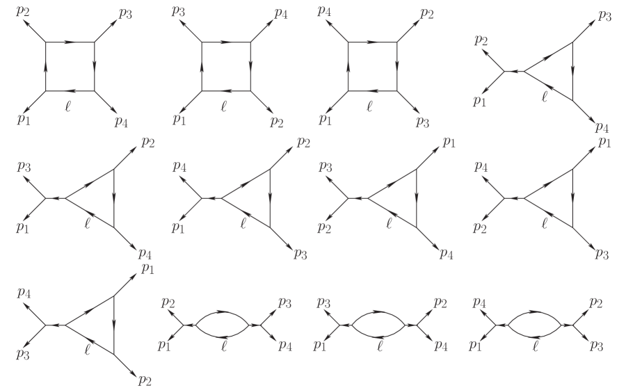
Figure 4: The contributing Feynman diagrams of non-color-ordered 4-point one-loop amplitude in $\phi^{3}$ theory.

The non-color-ordered 4-point one-loop amplitude in $\phi^{3}$ theory is more complicated, yet the discussion follows the same way as in previous subsections. The interaction term here is ${\phi^{3}/3!}$. The loop integrand gets contributions from three box diagrams, six triangle diagrams and three bubble diagrams, as shown in Figure (4), given by

$${\cal I}^{\mathcal{F}}={\cal I}^{\phi^{3}}_{\Box}+{\cal I}^{\phi^{3}}_{\triangle}+{\cal I}^{\phi^{3}}_{\between}~{},~{}~{}~{}$$ (48)

where

$${\cal I}_{\Box}^{\phi^{3}}={\cal I}^{\flat}_{\Box}(p_{1};p_{2};p_{3};p_{4})+{\cal I}^{\flat}_{\Box}(p_{1};p_{3};p_{4};p_{2})+{\cal I}^{\flat}_{\Box}(p_{1};p_{4};p_{2};p_{3})~{},~{}~{}~{}$$ (49)

$${\cal I}_{\triangle}^{\phi^{3}}={\cal I}^{\flat}_{\triangle}(p_{1},p_{2};p_{3};p_{4})+{\cal I}^{\flat}_{\triangle}(p_{1},p_{3};p_{2};p_{4})+{\cal I}^{\flat}_{\triangle}(p_{1},p_{4};p_{2};p_{3})$$

$$~{}~{}~{}~{}~{}~{}~{}+{\cal I}^{\flat}_{\triangle}(p_{2},p_{3};p_{1};p_{4})+{\cal I}^{\flat}_{\triangle}(p_{2},p_{4};p_{1};p_{3})+{\cal I}^{\flat}_{\triangle}(p_{3},p_{4};p_{1};p_{2})~{},~{}~{}~{}$$ (50)

$${\cal I}_{\between}^{\phi^{3}}={1\over 2}{\cal I}^{\flat}_{\between}(p_{1},p_{2};p_{3},p_{4})+{1\over 2}{\cal I}^{\flat}_{\between}(p_{1},p_{3};p_{2},p_{4})+{1\over 2}{\cal I}^{\flat}_{\between}(p_{1},p_{4};p_{2},p_{3})~{}.~{}~{}~{}$$ (51)

and the expressions of ${\cal I}^{\flat}_{\Box}(p_{1};p_{2};p_{3};p_{4})$, ${\cal I}^{\flat}_{\triangle}(p_{1},p_{2};p_{3};p_{4})$, ${\cal I}^{\flat}_{\between}(p_{1},p_{2};p_{3},p_{4})$ can be inferred from (18), (14) and (10). Again the semicolon separates external momenta consecutively onto each end of corresponding Feynman diagrams, and a symmetry factor $1/2$ is associated to each bubble diagram. Note that for box diagrams (or triangles), a diagram ${\cal I}_{\Box}^{\flat}(p_{1};p_{2};p_{3};p_{4})$ is topologically equivalent to its mirror reflection ${\cal I}_{\Box}^{\flat}(p_{1};p_{4};p_{3};p_{2})$ (or ${\cal I}_{\triangle}^{\flat}(p_{1};p_{2};p_{3})$ to ${\cal I}_{\triangle}^{\flat}(p_{1};p_{3};p_{2})$), so we must not over-count them.

The integrand in $\mathcal{Q}$-cut representation is given by

$${\cal I}^{\mathcal{Q}} = {1\over 2}{\cal A}_{L}(1,2,\widehat{\ell}_{R},-\widehat{\ell}_{L}){1\over\ell^{2}(-2\ell\cdot p_{12}+p_{12}^{2})}{\cal A}_{R}(\widehat{\ell}_{L},-\widehat{\ell}_{R},3,4)$$ (52)

$$+{1\over 2}{\cal A}_{L}(1,3,\widehat{\ell}_{R},-\widehat{\ell}_{L}){1\over\ell^{2}(-2\ell\cdot p_{13}+p_{13}^{2})}{\cal A}_{R}(\widehat{\ell}_{L},-\widehat{\ell}_{R},2,4)$$

$$+{1\over 2}{\cal A}_{L}(1,4,\widehat{\ell}_{R},-\widehat{\ell}_{L}){1\over\ell^{2}(-2\ell\cdot p_{14}+p_{14}^{2})}{\cal A}_{R}(\widehat{\ell}_{L},-\widehat{\ell}_{R},2,3)$$

$$+{1\over 2}{\cal A}_{L}(2,3,\widehat{\ell}_{R},-\widehat{\ell}_{L}){1\over\ell^{2}(-2\ell\cdot p_{23}+p_{23}^{2})}{\cal A}_{R}(\widehat{\ell}_{L},-\widehat{\ell}_{R},1,4)$$

$$+{1\over 2}{\cal A}_{L}(2,4,\widehat{\ell}_{R},-\widehat{\ell}_{L}){1\over\ell^{2}(-2\ell\cdot p_{24}+p_{24}^{2})}{\cal A}_{R}(\widehat{\ell}_{L},-\widehat{\ell}_{R},1,3)$$

$$+{1\over 2}{\cal A}_{L}(3,4,\widehat{\ell}_{R},-\widehat{\ell}_{L}){1\over\ell^{2}(-2\ell\cdot p_{34}+p_{34}^{2})}{\cal A}_{R}(\widehat{\ell}_{L},-\widehat{\ell}_{R},1,2)~{},~{}~{}~{}$$

where the $D$-dimensional non-color-ordered tree amplitude is given by

$${\cal A}_{L}(i,j,\widehat{\ell}_{R},-\widehat{\ell}_{L})={-\ell_{L}\cdot p_{ij}\over p_{ij}^{2}(\ell_{L}\cdot p_{i})}+{-\ell_{L}\cdot p_{ij}\over p_{ij}^{2}(\ell_{L}\cdot p_{j})}+{1\over p_{ij}^{2}}~{}.~{}~{}~{}$$ (53)

Hence we get

$${\cal I}^{\mathcal{Q}} = {1\over 2}\Big{(}{-\ell\cdot p_{12}\over p_{12}^{2}(\ell\cdot p_{1})}+{-\ell\cdot p_{12}\over p_{12}^{2}(\ell\cdot p_{2})}+{1\over p_{12}^{2}}\Big{)}{1\over\ell^{2}(-2\ell\cdot p_{12}+p_{12}^{2})}\Big{(}{-\ell\cdot p_{34}\over p_{34}^{2}(\ell\cdot p_{3})}+{-\ell\cdot p_{34}\over p_{34}^{2}(\ell\cdot p_{4})}+{1\over p_{34}^{2}}\Big{)}$$ (54)

$$+{1\over 2}\Big{(}{-\ell\cdot p_{13}\over p_{13}^{2}(\ell\cdot p_{1})}+{-\ell\cdot p_{13}\over p_{13}^{2}(\ell\cdot p_{3})}+{1\over p_{13}^{2}}\Big{)}{1\over\ell^{2}(-2\ell\cdot p_{13}+p_{13}^{2})}\Big{(}{-\ell\cdot p_{24}\over p_{24}^{2}(\ell\cdot p_{2})}+{-\ell\cdot p_{24}\over p_{24}^{2}(\ell\cdot p_{4})}+{1\over p_{24}^{2}}\Big{)}$$

$$+{1\over 2}\Big{(}{-\ell\cdot p_{14}\over p_{14}^{2}(\ell\cdot p_{1})}+{-\ell\cdot p_{14}\over p_{14}^{2}(\ell\cdot p_{4})}+{1\over p_{14}^{2}}\Big{)}{1\over\ell^{2}(-2\ell\cdot p_{14}+p_{14}^{2})}\Big{(}{-\ell\cdot p_{23}\over p_{23}^{2}(\ell\cdot p_{2})}+{-\ell\cdot p_{23}\over p_{23}^{2}(\ell\cdot p_{3})}+{1\over p_{23}^{2}}\Big{)}$$

$$+{1\over 2}\Big{(}{-\ell\cdot p_{23}\over p_{23}^{2}(\ell\cdot p_{2})}+{-\ell\cdot p_{23}\over p_{23}^{2}(\ell\cdot p_{3})}+{1\over p_{23}^{2}}\Big{)}{1\over\ell^{2}(-2\ell\cdot p_{23}+p_{23}^{2})}\Big{(}{-\ell\cdot p_{14}\over p_{14}^{2}(\ell\cdot p_{1})}+{-\ell\cdot p_{14}\over p_{14}^{2}(\ell\cdot p_{4})}+{1\over p_{14}^{2}}\Big{)}$$

$$+{1\over 2}\Big{(}{-\ell\cdot p_{24}\over p_{24}^{2}(\ell\cdot p_{2})}+{-\ell\cdot p_{24}\over p_{24}^{2}(\ell\cdot p_{4})}+{1\over p_{24}^{2}}\Big{)}{1\over\ell^{2}(-2\ell\cdot p_{24}+p_{24}^{2})}\Big{(}{-\ell\cdot p_{13}\over p_{13}^{2}(\ell\cdot p_{1})}+{-\ell\cdot p_{13}\over p_{13}^{2}(\ell\cdot p_{3})}+{1\over p_{13}^{2}}\Big{)}$$

$$+{1\over 2}\Big{(}{-\ell\cdot p_{34}\over p_{34}^{2}(\ell\cdot p_{3})}+{-\ell\cdot p_{34}\over p_{34}^{2}(\ell\cdot p_{4})}+{1\over p_{34}^{2}}\Big{)}{1\over\ell^{2}(-2\ell\cdot p_{34}+p_{34}^{2})}\Big{(}{-\ell\cdot p_{12}\over p_{12}^{2}(\ell\cdot p_{1})}+{-\ell\cdot p_{12}\over p_{12}^{2}(\ell\cdot p_{2})}+{1\over p_{12}^{2}}\Big{)}~{}.~{}~{}~{}$$

Now let us compare these two integrands directly at the integrand-level. As usual, we can rewrite ${\cal I}^{\mathcal{F}}={\cal I}_{\Box}^{\phi^{3}}+{\cal I}_{\triangle}^{\phi^{3}}+{\cal I}_{\between}^{\phi^{3}}$ into the $\mathcal{Q}$-cut form with (20), (16) and (13). However, the one-to-one correspondence is not manifest when in terms of the loop integrand of the form (48), since ${\cal I}^{\mathcal{Q}}$ is permutation invariant with respect to external momenta, while ${\cal I}^{\mathcal{F}}$ of the form (48) is not. Recall that a single box or triangle diagram is topologically equivalent to its mirror reflection, we can rewrite ${\cal I}^{\mathcal{F}}$ as

$${\cal I}_{\Box}^{\phi^{3}}={1\over 2}\Big{(}{\cal I}^{\flat}_{\Box}(p_{1};p_{2};p_{3};p_{4})+{\cal I}^{\flat}_{\Box}(p_{1};p_{3};p_{4};p_{2})+{\cal I}^{\flat}_{\Box}(p_{1};p_{4};p_{2};p_{3})$$

$$~{}~{}~{}~{}~{}~{}~{}~{}~{}~{}~{}~{}~{}~{}~{}~{}~{}~{}~{}~{}~{}~{}~{}~{}~{}~{}~{}~{}+{\cal I}^{\flat}_{\Box}(p_{1};p_{4};p_{3};p_{2})+{\cal I}^{\flat}_{\Box}(p_{1};p_{2};p_{4};p_{3})+{\cal I}^{\flat}_{\Box}(p_{1};p_{3};p_{2};p_{4})\Big{)}~{},~{}~{}~{}$$ (55)

$${\cal I}_{\triangle}^{\phi^{3}}={1\over 2}\Big{(}{\cal I}^{\flat}_{\triangle}(p_{1},p_{2};p_{3};p_{4})+{\cal I}^{\flat}_{\triangle}(p_{1},p_{3};p_{2};p_{4})+{\cal I}^{\flat}_{\triangle}(p_{1},p_{4};p_{2};p_{3})$$

$$~{}~{}~{}~{}~{}~{}~{}~{}~{}~{}~{}~{}~{}~{}~{}~{}~{}~{}~{}~{}~{}~{}~{}~{}~{}~{}~{}~{}~{}~{}~{}+{\cal I}^{\flat}_{\triangle}(p_{2},p_{3};p_{1};p_{4})+{\cal I}^{\flat}_{\triangle}(p_{2},p_{4};p_{1};p_{3})+{\cal I}^{\flat}_{\triangle}(p_{3},p_{4};p_{1};p_{2})$$

$$~{}~{}~{}~{}~{}~{}~{}~{}~{}~{}~{}~{}~{}+{\cal I}^{\flat}_{\triangle}(p_{1},p_{2};p_{4};p_{3})+{\cal I}^{\flat}_{\triangle}(p_{1},p_{3};p_{4};p_{2})+{\cal I}^{\flat}_{\triangle}(p_{1},p_{4};p_{3};p_{2})$$

$$~{}~{}~{}~{}~{}~{}~{}~{}~{}~{}~{}~{}~{}~{}~{}~{}~{}~{}~{}~{}~{}~{}~{}~{}~{}~{}~{}~{}~{}~{}~{}+{\cal I}^{\flat}_{\triangle}(p_{2},p_{3};p_{4};p_{1})+{\cal I}^{\flat}_{\triangle}(p_{2},p_{4};p_{3};p_{1})+{\cal I}^{\flat}_{\triangle}(p_{3},p_{4};p_{2};p_{1})\Big{)}~{},~{}~{}~{}$$ (56)

while ${\cal I}_{\between}^{\phi^{3}}$ remains the same. By rewriting this one can find that, after transforming ${\cal I}^{\mathcal{F}}$ with (20), (16) and (13), each term in ${\cal I}^{\mathcal{F}}$ has its correspondence in ${\cal I}^{\mathcal{Q}}$. An implicit evidence of the equivalence can be shown by counting the number of terms. Expanding ${\cal I}^{\mathcal{Q}}$ given by (54), we get 54 terms. Judged by the appearance of loop momentum $\ell$ in the denominator of each term, we can infer that 6 terms come from bubble diagrams, $4\times 6=24$ terms come from triangle diagrams and $4\times 6=24$ terms come from box diagrams. Meanwhile, ${\cal I}_{\between}^{\phi^{3}}$ gives $3\times 2=6$ terms, ${\cal I}_{\triangle}^{\phi^{3}}$ $12\times 2=24$ terms and ${\cal I}_{\Box}^{\phi^{3}}$ $6\times 4=24$ terms after expressed as $\mathcal{Q}$-cut forms with (20), (16) and (13), and the symmetry factor $1/2$ is exactly expected. Of course, the honest comparison can be done by explicitly expanding ${\cal I}^{\mathcal{Q}}$ and ${\cal I}^{\mathcal{F}}$, and comparing them one by one for all 54 terms, which indeed confirms the equivalence ${\cal I}^{\mathcal{F}}\simeq{\cal I}^{\mathcal{Q}}$.

Next we turn to the comparison by the unitarity cut. Taking $s_{12}$-cut channel as an example, for the contribution from ${\cal I}^{\mathcal{Q}}(\ell)$, we need to evaluate

$$\Delta^{\mathcal{Q}}_{s_{12}}=\int d^{4}\ell_{L}d^{4}\ell_{R}~{}\delta^{4}(\ell_{R}-\ell_{L}+p_{12})\delta^{+}(\ell_{L}^{2})\delta^{+}(\ell_{R}^{2})\times{\cal I}^{\mathcal{Q}}(\ell)~{}\ell_{L}^{2}\ell_{R}^{2}~{}.~{}~{}~{}$$ (57)

Identifying $\ell=\ell_{L}$ (or $\ell=\ell_{R}$) and integrating over $\ell_{R}$ (or $\ell_{L}$) against momentum conservation, we get respectively

$$\Delta^{\mathcal{Q}}_{s_{12}}[\ell_{L}] = \int d^{4}\ell_{L}~{}\delta^{+}(\ell_{L}^{2})\delta^{+}((\ell_{L}-p_{12})^{2}){1\over 2}\Big{(}{-\ell_{L}\cdot p_{12}\over p_{12}^{2}(\ell_{L}\cdot p_{1})}+{-\ell_{L}\cdot p_{12}\over p_{12}^{2}(\ell_{L}\cdot p_{2})}+{1\over p_{12}^{2}}\Big{)}\Big{(}{-\ell_{L}\cdot p_{34}\over p_{34}^{2}(\ell_{L}\cdot p_{3})}+{-\ell_{L}\cdot p_{34}\over p_{34}^{2}(\ell_{L}\cdot p_{4})}+{1\over p_{34}^{2}}\Big{)}$$ (58)

$$= \int d^{4}\ell_{L}~{}\delta^{+}(\ell_{L}^{2})\delta^{+}((\ell_{L}-p_{12})^{2}){1\over 2}\Big{(}-{1\over 2\ell_{L}\cdot p_{1}}-{1\over 2\ell_{L}\cdot p_{2}}+{1\over p_{12}^{2}}\Big{)}\Big{(}{1\over 2\ell_{L}\cdot p_{3}}+{1\over 2\ell_{L}\cdot p_{4}}+{1\over p_{34}^{2}}\Big{)}~{},~{}~{}~{}$$

and

$$\Delta^{\mathcal{Q}}_{s_{12}}[\ell_{R}] = \int d^{4}\ell_{R}~{}\delta^{+}(\ell_{R}^{2})\delta^{+}((\ell_{R}+p_{12})^{2}){1\over 2}\Big{(}{-\ell_{R}\cdot p_{34}\over p_{34}^{2}(\ell_{R}\cdot p_{3})}+{-\ell_{R}\cdot p_{34}\over p_{34}^{2}(\ell_{R}\cdot p_{4})}+{1\over p_{34}^{2}}\Big{)}\Big{(}{-\ell_{R}\cdot p_{12}\over p_{12}^{2}(\ell_{R}\cdot p_{1})}+{-\ell_{R}\cdot p_{12}\over p_{12}^{2}(\ell_{R}\cdot p_{2})}+{1\over p_{12}^{2}}\Big{)}$$ (59)

$$= \int d^{4}\ell_{R}~{}\delta^{+}(\ell_{R}^{2})\delta^{+}((\ell_{R}+p_{12})^{2}){1\over 2}\Big{(}-{1\over 2\ell_{R}\cdot p_{3}}-{1\over 2\ell_{R}\cdot p_{4}}+{1\over p_{34}^{2}}\Big{)}\Big{(}{1\over 2\ell_{R}\cdot p_{1}}+{1\over 2\ell_{R}\cdot p_{2}}+{1\over p_{12}^{2}}\Big{)}~{},~{}~{}~{}$$

where in the second line we have used the on-shell conditions $2\ell_{L}\cdot p_{12}=p_{12}^{2}$ and $2\ell_{L}\cdot p_{34}=p_{34}^{2}$ for $\Delta^{\mathcal{Q}}_{s_{12}}[\ell_{L}]$ and $\Delta^{\mathcal{Q}}_{s_{12}}[\ell_{R}]$ respectively.

The contribution of $s_{12}$-cut channel by sewing two on-shell tree amplitudes, after inserting the explicit expressions of 4-dimensional 4-point tree amplitudes, is given by

$$\Delta^{\mathcal{F}}_{s_{12}} = {1\over 2}\int d^{4}\ell_{L}d^{4}\ell_{R}~{}\delta^{4}(\ell_{R}-\ell_{L}+p_{12})\delta^{+}(\ell_{L}^{2})\delta^{+}(\ell_{R}^{2})$$ (60)

$$~{}~{}~{}~{}~{}~{}~{}~{}~{}~{}~{}~{}~{}~{}~{}~{}\times\Big{(}{1\over(\ell_{L}-p_{1})^{2}}+{1\over(\ell_{L}-p_{2})^{2}}+{1\over p_{12}^{2}}\Big{)}\Big{(}{1\over(\ell_{R}-p_{3})^{2}}+{1\over(\ell_{R}-p_{4})^{2}}+{1\over p_{34}^{2}}\Big{)}~{}.~{}~{}~{}$$

Note that the prefactor $1/2$ should be included for the double unitarity cut to avoid over-counting terms. Hence we have

$$\Delta^{\mathcal{F}}_{s_{12}}[\ell_{L}] = {1\over 2}\int d^{4}\ell_{L}~{}\delta^{+}(\ell_{L}^{2})\delta^{+}((\ell_{L}-p_{12})^{2})$$ (61)

$$~{}~{}~{}~{}~{}~{}~{}~{}~{}~{}~{}~{}~{}~{}~{}\times\Big{(}{1\over(\ell_{L}-p_{1})^{2}}+{1\over(\ell_{L}-p_{2})^{2}}+{1\over p_{12}^{2}}\Big{)}\Big{(}{1\over(\ell_{L}+p_{4})^{2}}+{1\over(\ell_{L}+p_{3})^{2}}+{1\over p_{34}^{2}}\Big{)}~{},~{}~{}~{}$$

as well as

$$\Delta^{\mathcal{F}}_{s_{12}}[\ell_{R}] = {1\over 2}\int d^{4}\ell_{R}~{}\delta^{+}(\ell_{R}^{2})\delta^{+}((\ell_{R}+p_{12})^{2})$$ (62)

$$~{}~{}~{}~{}~{}~{}~{}~{}~{}~{}~{}~{}~{}~{}~{}~{}\times\Big{(}{1\over(\ell_{R}+p_{2})^{2}}+{1\over(\ell_{R}+p_{1})^{2}}+{1\over p_{12}^{2}}\Big{)}\Big{(}{1\over(\ell_{R}-p_{3})^{2}}+{1\over(\ell_{R}-p_{4})^{2}}+{1\over p_{34}^{2}}\Big{)}~{}.~{}~{}~{}$$

Recall the on-shell cut conditions $\ell_{L}^{2}=0$, $\ell_{R}^{2}=0$ as well as the massless conditions $p_{i}^{2}=0$, we immediately find $\Delta^{\mathcal{Q}}_{s_{12}}[\ell_{L}]\simeq\Delta^{\mathcal{F}}_{s_{12}}[\ell_{L}]$ and $\Delta^{\mathcal{Q}}_{s_{12}}[\ell_{R}]\simeq\Delta^{\mathcal{F}}_{s_{12}}[\ell_{R}]$.

Discussion of $s_{13}$- and $s_{14}$-cut channels is entirely parallel to $s_{12}$-cut channel, where we only need to replace $\{p_{1},p_{2},p_{3},p_{4}\}\to\{p_{1},p_{3},p_{2},p_{4}\}$ for $s_{13}$ channel or $\{p_{1},p_{2},p_{3},p_{4}\}\to\{p_{4},p_{1},p_{2},p_{3}\}$ for $s_{14}$ channel. This trivially verifies the equivalence $\Delta^{\mathcal{Q}}_{s_{13}}[\ell_{L}]\simeq\Delta^{\mathcal{F}}_{s_{13}}[\ell_{L}]$, $\Delta^{\mathcal{Q}}_{s_{13}}[\ell_{R}]\simeq\Delta^{\mathcal{F}}_{s_{13}}[\ell_{R}]$ and $\Delta^{\mathcal{Q}}_{s_{14}}[\ell_{L}]\simeq\Delta^{\mathcal{F}}_{s_{14}}[\ell_{L}]$, $\Delta^{\mathcal{Q}}_{s_{14}}[\ell_{R}]\simeq\Delta^{\mathcal{F}}_{s_{14}}[\ell_{R}]$. Thus the equivalence ${\cal I}^{\mathcal{Q}}\simeq{\cal I}^{\mathcal{F}}$ is confirmed by that for each cut channel.

4 Applications in the Yang-Mills theory

In the previous section we illustrate the summation over all $\mathcal{Q}$-cuts with amplitudes of scalar field theories. In this section, we will clarify the summation over helicity states of internal particles with color-ordered amplitudes of the Yang-Mills theory. The convention adopted here is the t’Hooft-Veltman (HV) regularization scheme tHooft:1972fi , i.e., the loop momentum will be $(4-2\epsilon)$-dimensional (as well as the polarization vector) while the external momenta will be kept in the exact 4-dimension. More specifically, in the ${\cal Q}$-cut construction (2), $\widetilde{\ell}_{L}$ and $\widetilde{\ell}_{R}$ have non-vanishing components in the $(-2\epsilon)$-dimension. As mentioned before, under dimensional deformation, $\widehat{\ell}_{L}$ and $\widehat{\ell}_{R}$ will live in general $D$-dimension, so the on-shell tree amplitudes used in (2) should be the ones of $D$-dimension. These amplitudes can be computed by Feynman rules, or expressions generated by tree-level CHY formula Cachazo:2013gna ; Cachazo:2013hca ; Cachazo:2013iea ; Cachazo:2014nsa ; Cachazo:2014xea , or $D$-dimensional BCFW recursion relation Britto:2004ap ; Britto:2005fq . In this paper, we will only focus on the 4-point one-loop amplitudes, and the necessary 4-point pure gluon tree amplitudes under various combinations of helicity states $+,-,S_{A}$ are summarized in appendix B for reference. Furthermore, as emphasized in §2, while one can handle $\widehat{\ell}_{L}$ and $\widehat{\ell}_{R}$ in $D$-dimension, when summing over physical helicity states in (2), we should restrict to $(4-2\epsilon)$-dimension in order to produce the correct result.

4.1 Color-ordered 4-point gluon amplitude ${\cal A}^{\tiny\mbox{1-loop}}_{4}(1^{+},2^{+},3^{+},4^{+})$

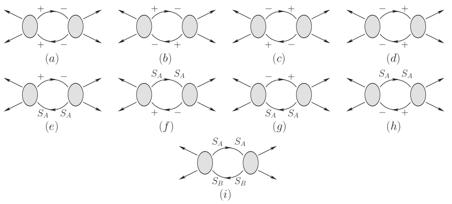
Figure 5: All possible internal states for the helicity sum of a given $\mathcal{Q}$-cut term, while the internal particles are $D$-dimensional gluons of $+,-$ and $S_{A}$ $(A=1,\ldots,\dim[\mu])$ physical polarizations.

Let us start with a relatively simple example, namely the 4-point gluon amplitude with all plus helicities $A_{4}^{\tiny\mbox{1-loop}}(1^{+},2^{+},3^{+},4^{+})$. For Yang-Mills theory, we will not compute one-loop integrands by using Feynman rules, but directly from ${\cal Q}$-cut construction and confirm its validity by the cross-check of the unitarity cut method.

According to (2), this loop integrand is given by

$${\cal I}^{\mathcal{Q}}(\widetilde{\ell})=\sum_{h_{1},h_{2}}{\cal A}_{L}(1^{+},2^{+},\widehat{\ell}_{R}^{~{}h_{1}},-\widehat{\ell}_{L}^{~{}h_{2}}){1\over\widetilde{\ell}^{2}}{1\over(-2\widetilde{\ell}\cdot p_{12}+p_{12}^{2})}{\cal A}_{R}(\widehat{\ell}_{L}^{~{}\bar{h}_{2}},-\widehat{\ell}_{R}^{~{}\bar{h}_{1}},3^{+},4^{+})+\mbox{Cyclic}\{p_{1},p_{2},p_{3},p_{4}\}~{},~{}~{}~{}$$ (63)

which contains four $\mathcal{Q}$-cut terms, and the helicities $h_{1},h_{2}$ of internal states should be summed in line with the nine cases shown in Figure (5). If the internal gluons are 4-dimensional, only the first four diagrams in Figure (5) may exist, which all vanish due to $A^{\tiny\mbox{tree}}_{4}(+,+,+,+)=0$, $A^{\tiny\mbox{tree}}_{4}(+,+,+,-)=0$ in 4-dimension. When the loop momentum is taken to be $D$-dimensional and all external momenta have positive helicities, the cases of Figure (5.a), (5.d), (5.e), (5.f), (5.g), (5.h) have no contribution due to the vanishing tree amplitudes. So we only need to sum over Figure (5.b), (5.c) and (5.i) with $S_{A}=S_{B}$, given by

$${\cal I}^{\mathcal{Q}}(\widetilde{\ell}) = {\cal A}_{L}(1^{+},2^{+},\widehat{\ell}_{R}^{~{}+},-\widehat{\ell}_{L}^{~{}-}){1\over\widetilde{\ell}^{2}}{1\over(-2\widetilde{\ell}\cdot p_{12}+p_{12}^{2})}{\cal A}_{R}(\widehat{\ell}_{L}^{~{}+},-\widehat{\ell}_{R}^{~{}-},3^{+},4^{+})$$ (64)

$$~{}~{}~{}~{}+{\cal A}_{L}(1^{+},2^{+},\widehat{\ell}_{R}^{~{}-},-\widehat{\ell}_{L}^{~{}+}){1\over\widetilde{\ell}^{2}}{1\over(-2\widetilde{\ell}\cdot p_{12}+p_{12}^{2})}{\cal A}_{R}(\widehat{\ell}_{L}^{~{}-},-\widehat{\ell}_{R}^{~{}+},3^{+},4^{+})$$

$$~{}~{}~{}~{}~{}~{}~{}~{}+\sum_{A}^{\dim[\mu]}{\cal A}_{L}(1^{+},2^{+},\widehat{\ell}_{R}^{~{}S_{A}},-\widehat{\ell}_{L}^{~{}S_{A}}){1\over\widetilde{\ell}^{2}}{1\over(-2\widetilde{\ell}\cdot p_{12}+p_{12}^{2})}{\cal A}_{R}(\widehat{\ell}_{L}^{~{}S_{A}},-\widehat{\ell}_{R}^{~{}S_{A}},3^{+},4^{+})$$

$$~{}~{}~{}~{}~{}~{}~{}~{}~{}~{}~{}~{}~{}~{}~{}~{}+\mbox{Cyclic}\{p_{1},p_{2},p_{3},p_{4}\}~{}.~{}~{}~{}$$

where again $\widehat{\ell}_{L}=\alpha_{L}(\widetilde{\ell}+\eta)$ and $\widetilde{\ell}=\ell+\mu$.

The $D$-dimensional tree amplitudes, as given in appendix B, depend on the reference momentum $q$. However for this example, the product ${\cal A}_{L}{\cal A}_{R}$ in each term is independent of $q$, thus the loop integrand is also independent of $q$, which serves as a consistency check. More explicitly, let us first write the general $D$-dimensional vector as $\widehat{\ell}_{L}\equiv(\widetilde{\ell},\eta)=(\ell,\mu,\eta)$, we have

$${\cal A}_{L}(1^{+},2^{+},\widehat{\ell}_{R}^{~{}+},-\widehat{\ell}_{L}^{~{}-}){\cal A}_{R}(\widehat{\ell}_{L}^{~{}+},-\widehat{\ell}_{R}^{~{}-},3^{+},4^{+})={[1~{}2][3~{}4]\over\langle 1~{}2\rangle\langle 3~{}4\rangle}{(\mu^{2}+\eta^{2})^{2}\over(2\widetilde{\ell}\cdot p_{1})(2\widetilde{\ell}\cdot p_{4})}~{},~{}~{}~{}$$ (65)

Under the massless conditions of $\widehat{\ell}_{L},\widehat{\ell}_{R}$, we should make the following replacement $\eta^{2}\to\widetilde{\ell}^{2}$ as well as $\widetilde{\ell}\to\alpha_{L}\widetilde{\ell}$ and $\mu\to\alpha_{L}\mu$ with $\alpha_{L}=p_{12}^{2}/(2\widetilde{\ell}\cdot p_{12})$ in succession, and find

$${\cal A}_{L}(1^{+},2^{+},\widehat{\ell}_{R}^{~{}+},-\widehat{\ell}_{L}^{~{}-}){\cal A}_{R}(\widehat{\ell}_{L}^{~{}+},-\widehat{\ell}_{R}^{~{}-},3^{+},4^{+})={[1~{}2][3~{}4]\over\langle 1~{}2\rangle\langle 3~{}4\rangle}{(\mu^{2}+\widetilde{\ell}^{2})^{2}(p_{12}^{2}/(2\widetilde{\ell}\cdot p_{12}))^{2}\over(2\widetilde{\ell}\cdot p_{1})(2\widetilde{\ell}\cdot p_{4})}~{}.~{}~{}~{}$$ (66)

The rest two diagrams

$${\cal A}_{L}(1^{+},2^{+},\widehat{\ell}_{R}^{~{}-},-\widehat{\ell}_{L}^{~{}+}){\cal A}_{R}(\widehat{\ell}_{L}^{~{}-},-\widehat{\ell}_{R}^{~{}+},3^{+},4^{+})~{}~{}\mbox{and}~{}~{}{\cal A}_{L}(1^{+},2^{+},\widehat{\ell}_{R}^{~{}S_{A}},-\widehat{\ell}_{L}^{~{}S_{A}}){\cal A}_{R}(\widehat{\ell}_{L}^{~{}S_{A}},-\widehat{\ell}_{R}^{~{}S_{A}},3^{+},4^{+})$$

lead to exactly the same results. Hence we get the integrand in $\mathcal{Q}$-cut representation as

$${\cal I}^{\mathcal{Q}}(\widetilde{\ell}) = (2-2\epsilon){[1~{}2][3~{}4]\over\langle 1~{}2\rangle\langle 3~{}4\rangle}{(\mu^{2}+\widetilde{\ell}^{2})^{2}(p_{12}^{2}/(2\widetilde{\ell}\cdot p_{12}))^{2}\over\widetilde{\ell}^{2}(-2\widetilde{\ell}\cdot p_{12}+p_{12}^{2})(2\widetilde{\ell}\cdot p_{1})(2\widetilde{\ell}\cdot p_{4})}+\mbox{Cyclic}\{p_{1},p_{2},p_{3},p_{4}\}~{},~{}~{}~{}$$ (67)

where we have summed over helicity states in $(4-2\epsilon)$-dimension (especially including the $S_{A}$ components in $\dim[\mu]=(-2\epsilon)$-dimension).

With this result, we can use the unitarity cut method to do the cross-check. Consider first the $s_{12}$-cut channel, we need to evaluate

$$\Delta^{\mathcal{Q}}_{s_{12}}=\int d^{4-2\epsilon}\widetilde{\ell}_{L}d^{4-2\epsilon}\widetilde{\ell}_{R}~{}\delta^{4-2\epsilon}(\widetilde{\ell}_{R}-\widetilde{\ell}_{L}+p_{12})\delta^{+}(\widetilde{\ell}_{L}^{~{}2})\delta^{+}(\widetilde{\ell}_{R}^{~{}2})\times{\cal I}^{\mathcal{Q}}(\widetilde{\ell})~{}\widetilde{\ell}_{L}^{~{}2}\widetilde{\ell}_{R}^{~{}2}~{}.~{}~{}~{}$$ (68)

Again we have two different choices of identifications. If we identify $\widetilde{\ell}=\widetilde{\ell}_{L}$ and integrate over $\widetilde{\ell}_{R}$ against momentum conservation, the factor $\widetilde{\ell}_{L}^{2}\widetilde{\ell}_{R}^{2}$ becomes $\widetilde{\ell}_{L}^{2}(\widetilde{\ell}_{L}-p_{12})^{2}\to\widetilde{\ell}_{L}^{2}(-2\widetilde{\ell}_{L}\cdot p_{12}+p_{12}^{2})$. Upon the cut conditions $\widetilde{\ell}_{L}^{2}=0$, $\widetilde{\ell}_{R}^{2}=0$, it trivially vanishes. Thus this picks out the terms with denominator $\widetilde{\ell}^{2}(-2\widetilde{\ell}\cdot p_{12}+p_{12}^{2})$ in (67) while all other terms vanish. Hence

$$\Delta^{\mathcal{Q}}_{s_{12}}[\widetilde{\ell}_{L}]=\int d^{4-2\epsilon}\widetilde{\ell}_{L}\delta^{+}(\widetilde{\ell}_{L}^{~{}2})\delta^{+}((\widetilde{\ell}_{L}-p_{12})^{2}){[1~{}2][3~{}4]\over\langle 1~{}2\rangle\langle 3~{}4\rangle}{(2-2\epsilon)\mu^{4}\over(2\widetilde{\ell}_{L}\cdot p_{1})(2\widetilde{\ell}_{L}\cdot p_{4})}~{}.~{}~{}~{}$$ (69)

If we identify $\widetilde{\ell}=\widetilde{\ell}_{R}$ and integrate over $\widetilde{\ell}_{L}$ against momentum conservation, only the terms with denominator $\widetilde{\ell}^{2}(-2\widetilde{\ell}\cdot p_{34}+p_{34}^{2})$ can survive. Thus we have

$$\Delta^{\mathcal{Q}}_{s_{12}}[\widetilde{\ell}_{R}]=\int d^{4-2\epsilon}\widetilde{\ell}_{R}~{}\delta^{+}(\widetilde{\ell}_{R}^{~{}2})\delta^{+}((\widetilde{\ell}_{R}+p_{12})^{2}){[3~{}4][1~{}2]\over\langle 3~{}4\rangle\langle 1~{}2\rangle}{(2-2\epsilon)\mu^{4}\over(2\widetilde{\ell}_{R}\cdot p_{3})(2\widetilde{\ell}_{R}\cdot p_{2})}~{}.~{}~{}~{}$$ (70)

For the $s_{12}$-channel, the standard unitarity cut method yields

$$\Delta^{\mathcal{F}}_{s_{12}} = \sum_{h_{1},h_{2}}\int d^{4-2\epsilon}\widetilde{\ell}_{L}d^{4-2\epsilon}\widetilde{\ell}_{R}~{}\delta^{4-2\epsilon}(\widetilde{\ell}_{R}-\widetilde{\ell}_{L}+p_{12})\delta^{+}(\widetilde{\ell}_{L}^{~{}2})\delta^{+}(\widetilde{\ell}_{R}^{~{}2})$$ (71)

$$~{}~{}~{}~{}~{}~{}~{}~{}~{}~{}~{}~{}~{}~{}~{}~{}~{}~{}~{}~{}~{}~{}~{}~{}~{}~{}~{}~{}~{}~{}~{}~{}~{}~{}~{}~{}~{}~{}~{}~{}\times{\cal A}_{L}(1,2,\widetilde{\ell}_{R}^{~{}h_{1}},-\widetilde{\ell}_{L}^{~{}h_{2}}){\cal A}_{R}(\widetilde{\ell}_{L}^{~{}\bar{h}_{2}},-\widetilde{\ell}_{R}^{~{}\bar{h}_{1}},3,4)~{},~{}~{}~{}$$

where again the tree amplitudes ${\cal A}_{L},{\cal A}_{R}$ are $(4-2\epsilon)$-dimensional and the helicity states should be summed over the nine diagrams in Figure (5). Inserting the results in appendix B, we get

$$\Delta^{\mathcal{F}}_{s_{12}} = \int d^{4-2\epsilon}\widetilde{\ell}_{L}d^{4-2\epsilon}\widetilde{\ell}_{R}~{}\delta^{4-2\epsilon}(\widetilde{\ell}_{R}-\widetilde{\ell}_{L}+p_{12})\delta^{+}(\widetilde{\ell}_{L}^{~{}2})\delta^{+}(\widetilde{\ell}_{R}^{~{}2}){[1~{}2][3~{}4]\over\langle 1~{}2\rangle\langle 3~{}4\rangle}{-(2-2\epsilon)\mu^{4}\over(\widetilde{\ell}_{L}-p_{1})^{2}(\widetilde{\ell}_{R}-p_{3})^{2}}~{}.~{}~{}~{}$$ (72)

Depending on the integration order of $\widetilde{\ell}_{R}$ and $\widetilde{\ell}_{L}$, it gives

$$\Delta^{\mathcal{F}}_{s_{12}}[\widetilde{\ell}_{L}] = \int d^{4-2\epsilon}\widetilde{\ell}_{L}~{}\delta^{+}(\widetilde{\ell}_{L}^{~{}2})\delta^{+}((\widetilde{\ell}_{L}-p_{12})^{2}){[1~{}2][3~{}4]\over\langle 1~{}2\rangle\langle 3~{}4\rangle}{-(2-2\epsilon)\mu^{4}\over(\widetilde{\ell}_{L}-p_{1})^{2}(\widetilde{\ell}_{L}+p_{4})^{2}}~{},~{}~{}~{}$$ (73)

or

$$\Delta^{\mathcal{F}}_{s_{12}}[\widetilde{\ell}_{R}] = \int d^{4-2\epsilon}\widetilde{\ell}_{R}~{}\delta^{+}(\widetilde{\ell}_{R}^{~{}2})\delta^{+}((\widetilde{\ell}_{R}+p_{12})^{2}){[1~{}2][3~{}4]\over\langle 1~{}2\rangle\langle 3~{}4\rangle}{-(2-2\epsilon)\mu^{4}\over(\widetilde{\ell}_{R}+p_{2})^{2}(\widetilde{\ell}_{R}-p_{3})^{2}}~{}.~{}~{}~{}$$ (74)

Upon the on-shell conditions $\widetilde{\ell}_{L}^{2}=0$, $\widetilde{\ell}_{R}^{2}=0$ and $p_{i}^{2}=0$, we have confirmed the equivalence $\Delta^{\mathcal{Q}}_{s_{12}}\simeq\Delta^{\mathcal{F}}_{s_{12}}$.

Since all external particles have positive helicities, the cross-check for $s_{14}$-channel can be easily done by shifting $p_{i}\to p_{i+1}$ in the previous computation.

4.2 Color-ordered 4-point gluon amplitude ${\cal A}^{\tiny\mbox{1-loop}}_{4}(1^{+},2^{+},3^{+},4^{-})$

Now let us consider a more complicated example ${\cal A}^{\tiny\mbox{1-loop}}_{4}(1^{+},2^{+},3^{+},4^{-})$. Its one-loop integrand produced by $\mathcal{Q}$-cut construction is

$${\cal I}^{\mathcal{Q}}(\widetilde{\ell})=\sum_{h_{1},h_{2}}{\cal A}_{L}(1^{+},2^{+},\widehat{\ell}_{R}^{~{}h_{1}},-\widehat{\ell}_{L}^{~{}h_{2}}){1\over\widetilde{\ell}^{2}}{1\over(-2\widetilde{\ell}\cdot p_{12}+p_{12}^{2})}{\cal A}_{R}(\widehat{\ell}_{L}^{~{}\bar{h}_{2}},-\widehat{\ell}_{R}^{~{}\bar{h}_{1}},3^{+},4^{-})+\mbox{Cyclic}\{p_{1},p_{2},p_{3},p_{4}\}~{}.~{}~{}~{}$$ (75)

The $D$-dimensional tree amplitudes can be referred in appendix B. We still need to sum over the nine diagrams in Figure (5). But those of Figure (5.a), (5.e), (5.f) have no contribution due to the vanishing tree amplitudes, while that of Figure (5.i) only contributes when $S_{A}=S_{B}$. Hence we have, for example,

$$\sum_{h_{1},h_{2}}{\cal A}_{L}(1^{+},2^{+},\widehat{\ell}_{R}^{~{}h_{1}},-\widehat{\ell}_{L}^{~{}h_{2}}){\cal A}_{R}(\widehat{\ell}_{L}^{~{}\bar{h}_{2}},-\widehat{\ell}_{R}^{~{}\bar{h}_{1}},3^{+},4^{-})$$

$$= \sum_{A=1}^{\dim[\mu]}\Big{(}{\cal A}_{L}(1^{+},2^{+},\widehat{\ell}_{R}^{~{}S_{A}},-\widehat{\ell}_{L}^{~{}S_{A}}){\cal A}_{R}(\widehat{\ell}_{L}^{~{}S_{A}},-\widehat{\ell}_{R}^{~{}S_{A}},3^{+},4^{-})\Big{)}+\sum_{A=1}^{\dim[\mu]}\Big{(}{\cal A}_{L}(1^{+},2^{+},\widehat{\ell}_{R}^{~{}-},-\widehat{\ell}_{L}^{~{}S_{A}}){\cal A}_{R}(\widehat{\ell}_{L}^{~{}S_{A}},-\widehat{\ell}_{R}^{~{}+},3^{+},4^{-})\Big{)}$$

$$+\sum_{A=1}^{\dim[\mu]}\Big{(}{\cal A}_{L}(1^{+},2^{+},\widehat{\ell}_{R}^{~{}S_{A}},-\widehat{\ell}_{L}^{~{}-}){\cal A}_{R}(\widehat{\ell}_{L}^{~{}+},-\widehat{\ell}_{R}^{~{}S_{A}},3^{+},4^{-})\Big{)}+{\cal A}_{L}(1^{+},2^{+},\widehat{\ell}_{R}^{~{}-},-\widehat{\ell}_{L}^{~{}-}){\cal A}_{R}(\widehat{\ell}_{L}^{~{}+},-\widehat{\ell}_{R}^{~{}+},3^{+},4^{-})$$

$$+{\cal A}_{L}(1^{+},2^{+},\widehat{\ell}_{R}^{~{}-},-\widehat{\ell}_{L}^{~{}+}){\cal A}_{R}(\widehat{\ell}_{L}^{~{}-},-\widehat{\ell}_{R}^{~{}+},3^{+},4^{-})+{\cal A}_{L}(1^{+},2^{+},\widehat{\ell}_{R}^{~{}+},-\widehat{\ell}_{L}^{~{}-}){\cal A}_{R}(\widehat{\ell}_{L}^{~{}+},-\widehat{\ell}_{R}^{~{}-},3^{+},4^{-})~{}.~{}~{}~{}$$

Different from the previous example, here each term ${\cal A}_{L}{\cal A}_{R}$ depends on the reference momentum $q$, which is the gauge choice for the polarization vector. However, after summing all terms we do get a $q$-independent result, namely

$$\sum_{h_{1},h_{2}}{\cal A}_{L}(1^{+},2^{+},\widehat{\ell}_{R}^{~{}h_{1}},-\widehat{\ell}_{L}^{~{}h_{2}}){\cal A}_{R}(\widehat{\ell}_{L}^{~{}\bar{h}_{2}},-\widehat{\ell}_{R}^{~{}\bar{h}_{1}},3^{+},4^{-})=(2-2\epsilon)\frac{(\mu^{2}+\eta^{2})[2~{}1]\langle 4|{\ell}_{L}|3]^{2}}{\langle 1~{}2\rangle\langle 3~{}4\rangle[4~{}3](2\widehat{\ell}_{L}\cdot p_{1})(2\widehat{\ell}_{L}\cdot p_{4})}~{}.~{}~{}~{}$$ (77)

The detailed computation of helicity sum can be referred in appendix C. This result is rather compact, yet it enjoys the advantage of the spinor-helicity formalism. Another expression in terms of the standard Mandelstam variables can be obtained after tensor reduction, given by

$$(2-2\epsilon)(\mu^{2}+\eta^{2}){[1~{}3]\langle 4|3|2]\over\langle 1~{}3\rangle\langle 2|3|4]}\Big{(}{s_{14}-s_{13}\over 4s_{14}s_{13}}+{s_{12}s_{14}+s_{12}(\widehat{\ell}_{L}\cdot p_{1})+2i\epsilon(\widehat{\ell}_{L},1,2,3)\over 8s_{14}s_{13}(\widehat{\ell}_{L}\cdot p_{4})}~{}~{}~{}~{}~{}$$ (78)

$$+{s_{12}s_{14}+2s_{13}(\mu^{2}+\eta^{2})+4i\epsilon(\widehat{\ell}_{L},1,2,3)\over 32s_{13}(\widehat{\ell}_{L}\cdot p_{1})(\widehat{\ell}_{L}\cdot p_{4})}+{s_{12}s_{14}^{2}+(s_{14}^{2}+s_{13}^{2})(\widehat{\ell}_{L}\cdot p_{4})-2(s_{13}-s_{14})i\epsilon(\widehat{\ell}_{L},1,2,3)\over 8s_{12}s_{14}s_{13}(\widehat{\ell}_{L}\cdot p_{1})}\Big{)}~{},~{}~{}~{}$$

where $s_{ij}\equiv p_{ij}^{2}$. To finally reach the ${\cal Q}$-cut representation, we can impose $\eta^{2}\to\widetilde{\ell}^{2}$, $\widetilde{\ell}\to\alpha_{L}\widetilde{\ell}$, $\mu\to\alpha_{L}\mu$ and $\alpha_{L}=p_{12}^{2}/(2\ell_{L}\cdot p_{12})$ for either (77) or (78). For simplicity, we choose the expression (77) and get

$${\cal I}^{\mathcal{Q}}(\widetilde{\ell}) = {(2-2\epsilon)\langle 4|\ell|3]^{2}(\mu^{2}+\widetilde{\ell}^{2})(p_{12}^{2}/(2\widetilde{\ell}\cdot p_{12})^{2})\over\langle 1~{}2\rangle^{2}\widetilde{\ell}^{2}(-2\widetilde{\ell}\cdot p_{12}+p_{12}^{2})(2\widetilde{\ell}\cdot p_{1})(2\widetilde{\ell}\cdot p_{4})}+{(2-2\epsilon)\langle 4|\ell|1]^{2}(\mu^{2}+\widetilde{\ell}^{2})(p_{23}^{2}/(2\widetilde{\ell}\cdot p_{23})^{2})\over\langle 2~{}3\rangle^{2}\widetilde{\ell}^{2}(-2\widetilde{\ell}\cdot p_{23}+p_{23}^{2})(2\widetilde{\ell}\cdot p_{2})(2\widetilde{\ell}\cdot p_{1})}$$ (79)

$$+{(2-2\epsilon)\langle 4|\ell|3]^{2}(\mu^{2}+\widetilde{\ell}^{2})(p_{34}^{2}/(2\widetilde{\ell}\cdot p_{34})^{2})\over\langle 1~{}2\rangle^{2}\widetilde{\ell}^{2}(-2\widetilde{\ell}\cdot p_{34}+p_{34}^{2})(2\widetilde{\ell}\cdot p_{3})(2\widetilde{\ell}\cdot p_{2})}+{(2-2\epsilon)\langle 4|\ell|1]^{2}(\mu^{2}+\widetilde{\ell}^{2})(p_{41}^{2}/(2\widetilde{\ell}\cdot p_{41})^{2})\over\langle 2~{}3\rangle^{2}\widetilde{\ell}^{2}(-2\widetilde{\ell}\cdot p_{41}+p_{41}^{2})(2\widetilde{\ell}\cdot p_{4})(2\widetilde{\ell}\cdot p_{3})}~{}.~{}~{}~{}$$

In fact, by using identities

$$\Big{(}{p_{ij}^{2}\over 2\widetilde{\ell}\cdot p_{ij}}\Big{)}^{2}={(p_{ij}^{2}-2\widetilde{\ell}\cdot p_{ij}+2\widetilde{\ell}\cdot p_{ij})^{2}\over(2\widetilde{\ell}\cdot p_{ij})^{2}}={(p_{ij}^{2}-2\widetilde{\ell}\cdot p_{ij})^{2}\over(2\widetilde{\ell}\cdot p_{ij})^{2}}+{2(p_{ij}^{2}-2\widetilde{\ell}\cdot p_{ij})\over(2\widetilde{\ell}\cdot p_{ij})}+1~{},~{}~{}~{}$$ (80)

the factors $(p_{ij}^{2}/(2\widetilde{\ell}\cdot p_{ij}))^{2}$ can be effectively replaced by 1 after dropping scale-free terms, which simplifies the result into

$${\cal I}^{\mathcal{Q}}(\widetilde{\ell}) = {(2-2\epsilon)\langle 4|\ell|3]^{2}(\mu^{2}+\widetilde{\ell}^{2})\over\langle 1~{}2\rangle^{2}\widetilde{\ell}^{2}(-2\widetilde{\ell}\cdot p_{12}+p_{12}^{2})(2\widetilde{\ell}\cdot p_{1})(2\widetilde{\ell}\cdot p_{4})}+{(2-2\epsilon)\langle 4|\ell|1]^{2}(\mu^{2}+\widetilde{\ell}^{2})\over\langle 2~{}3\rangle^{2}\widetilde{\ell}^{2}(-2\widetilde{\ell}\cdot p_{23}+p_{23}^{2})(2\widetilde{\ell}\cdot p_{2})(2\widetilde{\ell}\cdot p_{1})}$$ (81)

$$+{(2-2\epsilon)\langle 4|\ell|3]^{2}(\mu^{2}+\widetilde{\ell}^{2})\over\langle 1~{}2\rangle^{2}\widetilde{\ell}^{2}(-2\widetilde{\ell}\cdot p_{34}+p_{34}^{2})(2\widetilde{\ell}\cdot p_{3})(2\widetilde{\ell}\cdot p_{2})}+{(2-2\epsilon)\langle 4|\ell|1]^{2}(\mu^{2}+\widetilde{\ell}^{2})\over\langle 2~{}3\rangle^{2}\widetilde{\ell}^{2}(-2\widetilde{\ell}\cdot p_{41}+p_{41}^{2})(2\widetilde{\ell}\cdot p_{4})(2\widetilde{\ell}\cdot p_{3})}~{}.~{}~{}~{}$$

Now we use the unitarity cut method to do the cross-check for this result, followed by the same strategy in the previous examples. For the $s_{12}$ channel, the computation of

$$\Delta^{\mathcal{Q}}_{s_{12}}=\int d^{4-2\epsilon}\widetilde{\ell}_{L}d^{4-2\epsilon}\widetilde{\ell}_{R}~{}\delta^{4-2\epsilon}(\widetilde{\ell}_{R}-\widetilde{\ell}_{L}+p_{12})\delta^{+}(\widetilde{\ell}_{L}^{~{}2})\delta^{+}(\widetilde{\ell}_{R}^{~{}2})\times{\cal I}^{\mathcal{Q}}(\widetilde{\ell})~{}\widetilde{\ell}_{L}^{~{}2}\widetilde{\ell}_{R}^{~{}2}~{}~{}~{}~{}$$ (82)

can be done by either identifying $\widetilde{\ell}=\widetilde{\ell}_{L}$ and integrating over $\widetilde{\ell}_{R}$, or identifying $\widetilde{\ell}=\widetilde{\ell}_{R}$ and integrating over $\widetilde{\ell}_{L}$. For the former choice, the first term in (81) is picked out, and the on-shell conditions $\widetilde{\ell}_{L}^{2}=0$, $\widetilde{\ell}_{R}^{2}=0$ imply $p_{12}^{2}/(2\widetilde{\ell}\cdot p_{12})=1$, hence

$$\Delta^{\mathcal{Q}}_{s_{12}}[\widetilde{\ell}_{L}]=\int d^{4-2\epsilon}\widetilde{\ell}_{L}\delta^{+}(\widetilde{\ell}_{L}^{~{}2})\delta^{+}((\widetilde{\ell}_{L}-p_{12})^{2}){\langle 4|\ell_{L}|3]^{2}\over\langle 1~{}2\rangle^{2}}{(2-2\epsilon)\mu^{2}\over(2\widetilde{\ell}_{L}\cdot p_{1})(2\widetilde{\ell}_{L}\cdot p_{4})}~{}.~{}~{}~{}$$ (83)

For the latter one, we have

$$\Delta^{\mathcal{Q}}_{s_{12}}[\widetilde{\ell}_{R}]=\int d^{4-2\epsilon}\widetilde{\ell}_{R}~{}\delta^{+}(\widetilde{\ell}_{R}^{~{}2})\delta^{+}((\widetilde{\ell}_{R}+p_{12})^{2}){\langle 4|\ell_{L}|3]^{2}\over\langle 1~{}2\rangle^{2}}{(2-2\epsilon)\mu^{2}\over(2\widetilde{\ell}_{R}\cdot p_{3})(2\widetilde{\ell}_{R}\cdot p_{2})}~{}.~{}~{}~{}$$ (84)

The traditional unitarity cut method gives the following result by sewing two $(4-2\epsilon)$-dimensional tree amplitudes, which is

$$\Delta^{\mathcal{F}}_{s_{12}} = \int d^{4-2\epsilon}\widetilde{\ell}_{L}d^{4-2\epsilon}\widetilde{\ell}_{R}~{}\delta^{4-2\epsilon}(\widetilde{\ell}_{R}-\widetilde{\ell}_{L}+p_{12})\delta^{+}(\widetilde{\ell}_{L}^{~{}2})\delta^{+}(\widetilde{\ell}_{R}^{~{}2}){\langle 4|\ell_{L}|3]^{2}\over\langle 1~{}2\rangle^{2}}{-(2-2\epsilon)\mu^{4}\over(\widetilde{\ell}_{L}-p_{1})^{2}(\widetilde{\ell}_{R}-p_{3})^{2}}~{}.~{}~{}~{}$$ (85)

Just like the computation in the previous subsection, depending on the integration order of $\widetilde{\ell}_{L}$ and $\widetilde{\ell}_{R}$, it can be immediately shown that $\Delta_{s_{12}}^{\mathcal{Q}}\simeq\Delta_{s_{12}}^{\mathcal{F}}$. Similar computation can be done for $s_{14}$-channel. Since for each unitarity cut the equivalence is valid, the equivalence between the loop integrands of ${\cal Q}$-cut representation and traditional Feynman diagrams has been confirmed.

5 Conclusion

In this paper, we take the integrands of one-loop amplitudes in scalar field and Yang-Mills theories as examples to elaborate various aspects of the newly proposed ${\cal Q}$-cut construction, specifically the summation over distinct $\mathcal{Q}$-cuts, as well as the internal helicity states. Furthermore, a cross-check using traditional unitarity cut has been provided, establishing the connection between this new algorithm and traditional computational techniques for loop amplitudes.

The construction of one-loop integrands has become a popular topic recently, by generalizing the tree-level massless on-shell CHY formulation Cachazo:2013hca ; Cachazo:2013iea to loop-level Geyer:2015bja , using the ambitwistor string theory (see also Baadsgaard:2015hia ; He:2015yua ). Furthermore, the authors of ref. Geyer:2015jch showed that their result was in fact equivalent to the $\mathcal{Q}$-cut representation, which is an affirmative support of this approach.

As also pointed out in Baadsgaard:2015twa , there are many questions to be investigated. First of all, it will be extremely significant to compute a non-trivial two-loop amplitude via the $\mathcal{Q}$-cut construction, to test its ability and potential advantages over other methods. Although the general framework to handle two or more loops has been prescribed, carrying out the particulars is unquestionably favorable. Secondly, the ideas encoded in the ${\cal Q}$-cut construction, especially the use of linear propagators, possibly opens a new window for the current researches on the integrand-level reduction by computational algebraic geometry method, or the integral-level reduction by improved IBP relations. It is worth exploring whether these two multi-loop integrand reduction techniques can be applied directly to the $\mathcal{Q}$-cut representation. Finally, at this moment, the ${\cal Q}$-cut construction is still restricted to massless theories, so it will be naturally important to generalize it to massive theories.

Appendix A Helicity choices of polarization vectors

Throughout this paper, we use the $D$-dimensional metric $\eta_{\mu\nu}=\mbox{diag}(+,-,-,\cdots,-)$. After cutting two internal lines of a one-loop diagram, we shall get two on-shell tree amplitudes, and each has two legs corresponding to the cut propagators in $D$-dimension. To describe such amplitudes, we define

$$\widehat{\ell}=(\ell,\vec{\mu})~{}~{}~{},~{}~{}~{}\vec{\mu}=(\mu_{1},\ldots,\mu_{d})~{},~{}~{}~{}$$ (86)

where $\ell$ is the 4-dimensional component and $\vec{\mu}$ is a vector in the extra $d$-dimension ($d=D-4$). For the Euclidean $d$-dimensional space, we adopt the basis $e_{A}$ with $A=1,...,d$ such that its components $\mu_{i}=\delta_{iA}$ for $i=1,...,d$. The massless condition of $\widehat{\ell}$ is then $\ell^{2}-\vec{\mu}^{2}=0$.

Now we define the polarization vectors along with the massless momentum $\widehat{\ell}$. The transverse condition $\epsilon\cdot\widehat{\ell}=0$ tells that the transverse space is $(D-2)$-dimensional. However, due to the gauge degree of freedom $\epsilon_{i}\sim\epsilon_{i}+{\alpha}\ell$, to completely fix $\epsilon_{i}$ we need to introduce an auxiliary momentum $q$, which corresponds to the gauge choice. For convenience, we will choose $q$ to be null in 4-dimension and $q\cdot\ell\neq 0$. With this choice, we can fix transverse polarization vectors by imposing the extra condition $\epsilon_{i}\cdot q=0$. According to the principles above, firstly, we define the null 4-dimensional momentum as

$$\ell^{\bot}=\ell-{\vec{\mu}^{2}\over\left\langle q|\ell|q\right]}q~{}~{}~{},~{}~{}~{}~{}({\ell^{\bot}})^{2}=0~{},~{}~{}~{}$$ (87)

where $\ell$ is the 4-dimensional component of $\widehat{\ell}$ (see (86)). With the null momentum $\ell^{\bot}$, the transverse polarization vectors can be defined as

$$\epsilon^{+}(\widehat{\ell},q)=\Big{(}{\langle q|\gamma_{\nu}|\ell^{\bot}]\over\sqrt{2}\langle q~{}\ell^{\bot}\rangle},\vec{0}_{d}\Big{)}~{}~{}~{},~{}~{}~{}\epsilon^{-}(\widehat{\ell},q)=\Big{(}{\langle\ell^{\bot}|\gamma_{\nu}|q]\over\sqrt{2}[\ell^{\bot}~{}q]},\vec{0}_{d}\Big{)}~{},~{}~{}~{}$$

$$\epsilon^{S_{A}}(\widehat{\ell},q)=\Big{(}{2\mu_{A}\over\langle q|\ell|q]}q,e_{A}\Big{)}~{}~{}~{},~{}~{}~{}A=1,...,d~{},~{}~{}~{}$$ (88)

where $\vec{0}$ denotes the $d$-dimensional vanishing vector, $e_{A}$ is the basis vector of the extra $d$-dimension and $\mu_{A}$ is the $A$-th component of $\vec{\mu}$ in (86). The reason of regarding $S_{A}$ as a superscript is that these polarization states behave like scalars with respect to the 4-dimension. The rest two polarization vectors are longitudinal and time-like, defined as

$$\epsilon^{L}(\widehat{\ell},q)=\widehat{\ell}~{}~{}~{},~{}~{}~{}\epsilon^{T}(\widehat{\ell},q)=(q,\vec{0}_{d})~{}.~{}~{}~{}$$ (89)

These $D$ polarization vectors possess the following relations

$$\epsilon^{\pm}\cdot q=\epsilon^{\pm}\cdot\ell=\epsilon^{\pm}\cdot\epsilon^{\pm}=0~{}~{},~{}~{}\epsilon^{+}\cdot\epsilon^{-}=-1~{},~{}~{}~{}$$

$$\epsilon^{L}\cdot\epsilon^{T}=\langle q|{\ell}|q]~{}~{},~{}~{}\epsilon^{S_{A}}\cdot\epsilon^{L,T}=0~{}~{},~{}~{}\epsilon^{S_{A}}\epsilon^{S_{B}}=-\delta^{AB}~{}.~{}~{}~{}$$ (90)

With this setup, we have the metric decomposition

$$\eta_{\mu\nu}={\epsilon^{L}\epsilon^{T}+\epsilon^{T}\epsilon^{L}\over\langle q|{\ell}|q]}-\epsilon^{+}\epsilon^{-}-\epsilon^{-}\epsilon^{+}-\sum_{A=1}^{d}\epsilon^{S_{A}}\epsilon^{S_{A}}~{}.~{}~{}~{}~{}~{}$$ (91)

The convention above is for general integer dimension $D$, but of course it can be trivially generalized to $(4-2\epsilon)$-dimension, for which we should replace $d\to-2\epsilon$.

Appendix B $D$-dimensional 4-point tree amplitudes of the Yang-Mills theory

The computation of loop integrands by $\mathcal{Q}$-cut representation requires on-shell tree amplitudes in general $D$-dimension. There are several ways to get these amplitudes. The first one is to use Feynman diagrams. The second one is to use the CHY formula, which holds in arbitrary dimensions Cachazo:2013hca ; Cachazo:2013iea . The third one is to use the on-shell recursion relation Britto:2004ap ; Britto:2005fq , starting from the 3-point seed amplitudes. Note that, for our formalism which involves extra dimensions and parameters, it is no longer obvious to get the 3-point amplitudes solely by little group scaling. Therefore conservatively, we still start from listing the 3-point amplitudes given by simple Feynman rules,

$${\cal A}(1,2,3) =-i\sqrt{2}\,\big{[}(p_{2}\cdot\epsilon_{3})(\epsilon_{1}\cdot\epsilon_{2})+(p_{3}\cdot\epsilon_{1})(\epsilon_{2}\cdot\epsilon_{3})+(p_{1}\cdot\epsilon_{2})(\epsilon_{3}\cdot\epsilon_{1})\big{]}~{}.~{}~{}~{}$$ (92)

For physical polarizations $+,-,S_{A}$ $(A=1,2,\ldots,d)$, we need the following 3-point tree amplitudes,

$${\cal A}_{3}(1^{+},2^{+},3^{+})=A(1^{-},2^{-},3^{-})=0~{}~{},~{}~{}{\cal A}_{3}(1^{+},2^{+},3^{-})=-{[1~{}2]^{3}\over[2~{}3][3~{}1]}~{}~{},~{}~{}{\cal A}_{3}(1^{-},2^{-},3^{+})={\langle 1~{}2\rangle^{3}\over\langle 2~{}3\rangle\langle 3~{}1\rangle}~{},~{}~{}~{}$$

$${\cal A}_{3}(1^{+},2^{+},3^{S_{A}})={\cal A}_{3}(1^{-},2^{-},3^{S_{A}})=0~{}~{},~{}~{}{\cal A}_{3}(1^{+},2^{-},3^{S_{A}})=\sqrt{2}\mu_{3A}{\langle 2~{}3\rangle[3~{}1]^{2}\over\langle 1~{}2\rangle[1~{}2][2~{}3]}~{},~{}~{}~{}$$

$${\cal A}_{3}(1^{S_{A}},2^{S_{B}},3^{+})=\delta^{AB}{[2~{}3][3~{}1]\over[1~{}2]}~{}~{},~{}~{}{\cal A}_{3}(1^{S_{A}},2^{S_{B}},3^{-})=-\delta^{AB}{\langle 2~{}3\rangle\langle 3~{}1\rangle\over\langle 1~{}2\rangle}~{},~{}~{}~{}$$

$${\cal A}_{3}(1^{S_{A}},2^{S_{B}},3^{S_{C}})=\sqrt{2}\Big{(}\delta^{AB}\mu_{3C}{\langle q|2|q]\over\langle q|3|q]}+\delta^{BC}\mu_{1A}{\langle q|3|q]\over\langle q|1|q]}+\delta^{CA}\mu_{2B}{\langle q|1|q]\over\langle q|2|q]}\Big{)}~{},~{}~{}~{}$$ (93)

where $\mu_{iA}$ is the $(4+A)$-th component of $p_{i}$ (or the $A$-th component in $d$-dimension), and $|p_{i}\rangle,|p_{i}]$ are understood to be $|p_{i}^{\bot}\rangle,|p_{i}^{\bot}]$ whenever $p_{i}$ is a $D$-dimensional momentum as defined in (87). With these inputs, we can get all tree amplitudes by BCFW recursion relation. For simplicity, we prefer to deform a pair of momenta which are 4-dimensional. Particularly, in this paper, we need 4-point tree amplitudes with two momenta $p_{1},p_{2}$ in 4-dimension and the rest two $p_{3},p_{4}$ in $D$-dimension. The deformation pair $\langle 1^{+}|2]$ would suffice to compute all required amplitudes without missing any boundary contribution. To illustrate this, let us compute ${\cal A}_{4}^{\tiny\mbox{tree}}(1^{+},2^{+},3^{+},4^{-})$ for example. Under $\langle 1|2]$ deformation, there is only one contribution

$${\cal A}_{3}(4^{-},\widehat{1}^{-},-\widehat{P}_{41}^{+}){1\over s_{41}}{\cal A}_{3}(\widehat{P}_{41}^{-},\widehat{2}^{+},3^{+})~{},~{}~{}~{}$$

and the deformed quantities are

$$|\widehat{1}\rangle=|1\rangle-{P_{41}^{2}\over\langle 2|P_{41}|1]}|2\rangle~{}~{},~{}~{}|\widehat{2}]=|2]+{P_{41}^{2}\over\langle 2|P_{41}|1]}|1]~{}~{},~{}~{}|\widehat{P}_{41}\rangle[\widehat{P}_{41}|={P_{41}|1]\langle 2|P_{41}\over\langle 2|P_{41}|1]}~{},~{}~{}~{}$$

therefore

$${\cal A}^{\tiny\mbox{tree}}_{4}(1^{+},2^{+},3^{+},4^{-})={[1~{}\widehat{P}_{41}]^{3}\over[\widehat{P}_{41}~{}4^{\bot}][4^{\bot}~{}1]}{1\over s_{14}}{[\widehat{2}~{}3^{\bot}]^{3}\over[3^{\bot}~{}\widehat{P}_{41}][\widehat{P}_{41}~{}\widehat{2}]}={\mu^{2}\over\langle 1|4|1]}{[2~{}1]\langle q~{}4^{\bot}\rangle^{2}\over\langle 1~{}2\rangle\langle q~{}3^{\bot}\rangle^{2}}~{}.~{}~{}~{}$$

For reader’s reference, here we list all necessary 4-point tree amplitudes with two 4-dimensional momenta denoted as $p_{1},p_{2}$ and two $D$-dimensional momenta denoted as $\widehat{\ell}_{1},\widehat{\ell}_{2}$. The polarization of $p_{i}$ can be either $+$ or $-$, while for $\widehat{\ell}_{i}$ it can be $+$, $-$ or $S_{A}$. Explicitly, without any $S$-component, we have

$${\cal A}_{4}(1^{+},2^{+},\widehat{\ell}_{2}^{~{}+},\widehat{\ell}_{1}^{~{}+}) = 0~{}~{}~{},~{}~{}~{}{\cal A}_{4}(1^{+},2^{+},\widehat{\ell}_{2}^{~{}+},\widehat{\ell}_{1}^{~{}-})={\mu^{2}\langle\ell_{1}^{\bot}~{}q\rangle^{2}[2~{}1]\over\langle\ell_{2}^{\bot}~{}q\rangle^{2}\langle 1~{}2\rangle\langle 2|{\ell}_{2}|2]}~{},~{}~{}~{}$$

$${\cal A}_{4}(1^{+},2^{+},\widehat{\ell}_{2}^{~{}-},\widehat{\ell}_{1}^{~{}-}) = -{\langle\ell_{1}^{\bot}~{}\ell_{2}^{\bot}\rangle^{2}[2~{}1]\over\langle 1~{}2\rangle\langle 2|{\ell}_{2}|2]}~{},~{}~{}~{}$$ (94)

and

$${\cal A}_{4}(1^{+},2^{-},\widehat{\ell}_{2}^{~{}+},\widehat{\ell}_{1}^{~{}+}) = {\mu^{2}~{}\left\langle q~{}2\right\rangle^{4}[2~{}1]\over\left\langle\ell_{1}^{\bot}~{}q\right\rangle^{2}\langle\ell_{2}^{\bot}~{}q\rangle^{2}\langle 1~{}2\rangle\langle 2|{\ell}_{2}|2]}~{}~{},~{}~{}{\cal A}_{4}(1^{+},2^{-},\widehat{\ell}_{2}^{~{}-},\widehat{\ell}_{1}^{~{}-})={\mu^{2}~{}\langle 1~{}2\rangle[1~{}q]^{4}\over\langle 2|\widehat{\ell}_{2}|2][q~{}\ell_{1}^{\bot}]^{2}[q~{}\ell_{2}^{\bot}]^{2}[2~{}1]}~{},~{}~{}~{}$$

$${\cal A}_{4}(1^{+},2^{-},\widehat{\ell}_{2}^{~{}+},\widehat{\ell}_{1}^{~{}-}) = {\big{(}\langle 1~{}2\rangle[1~{}\ell_{2}^{\bot}][1~{}q]-\langle 2|\widehat{\ell}_{2}|1][q~{}\ell_{2}^{\bot}]\big{)}\big{(}\langle\ell_{1}^{\bot}~{}q\rangle\langle 2|\widehat{\ell}_{1}|1]+\langle\ell_{1}^{\bot}~{}2\rangle\langle q~{}2\rangle[2~{}1]\big{)}\over\langle\ell_{2}^{\bot}~{}q\rangle\langle 1~{}2\rangle\langle 2|{\ell}_{2}|2][q~{}\ell_{1}^{\bot}][2~{}1]}~{}.~{}~{}~{}$$ (95)

With one $S$-component we have

$${\cal A}_{4}(1^{+},2^{+},\widehat{\ell}_{2}^{~{}+},\widehat{\ell}_{1}^{~{}S_{A}}) = 0~{}~{}~{},~{}~{}~{}{\cal A}_{4}(1^{+},2^{+},\widehat{\ell}_{2}^{~{}-},\widehat{\ell}_{1}^{~{}S_{A}})={\sqrt{2}\mu_{A}\langle\ell_{1}^{\bot}~{}\ell_{2}^{\bot}\rangle\langle\ell_{2}^{\bot}~{}q\rangle[2~{}1]\over\langle\ell_{1}^{\bot}~{}q\rangle\langle 1~{}2\rangle\langle 2|{\ell}_{2}|2]}~{},~{}~{}~{}$$

$${\cal A}_{4}(1^{+},2^{-},\widehat{\ell}_{2}^{~{}+},\widehat{\ell}_{1}^{~{}S_{A}}) = {\sqrt{2}\mu_{A}~{}\langle q~{}2\rangle^{2}\big{(}\langle 1~{}2\rangle[1~{}\ell_{2}^{\bot}][1~{}q]-\langle 2|\widehat{\ell}_{2}|1][q~{}\ell_{2}^{\bot}]\big{)}\over\langle\ell_{2}^{\bot}~{}q\rangle\langle 1~{}2\rangle\langle q|{\ell}_{1}|q]\langle 2|{\ell}_{2}|2]}~{},~{}~{}~{}$$

$${\cal A}_{4}(1^{+},2^{-},\widehat{\ell}_{2}^{~{}-},\widehat{\ell}_{1}^{~{}S_{A}}) = {\sqrt{2}\mu_{A}~{}[1~{}q]^{2}\big{(}\langle\ell_{2}^{\bot}~{}2\rangle\langle q~{}2\rangle[2~{}1]+\langle\ell_{2}^{\bot}~{}q\rangle\langle 2|\widehat{\ell}_{2}|1]\big{)}\over\langle q|{\ell}_{1}|q]\langle 2|{\ell_{2}}|2][q~{}\ell_{2}^{\bot}][2~{}1]}~{}.~{}~{}~{}$$ (96)

With two $S$-components we have

$${\cal A}_{4}(1^{+},2^{+},\widehat{\ell}_{2}^{~{}S_{A}},\widehat{\ell}_{1}^{~{}S_{B}}) = -{\mu^{2}[2~{}1]\over\langle 1~{}2\rangle\langle 2|{\ell}_{2}|2]}\delta^{AB}~{},~{}~{}~{}$$

$${\cal A}_{4}(1^{+},2^{-},\widehat{\ell}_{2}^{~{}S_{A}},\widehat{\ell}_{1}^{~{}S_{A}}) = -{2\mu_{A}^{2}~{}\langle q~{}2\rangle^{2}[1~{}q]^{2}\over\langle q|{\ell}_{1}|q]\langle q|{\ell}_{2}|q]\langle 2|\widehat{\ell}_{2}|2]}-{\langle 2|\widehat{\ell}_{1}|1]\langle 2|\widehat{\ell}_{2}|1]\over\langle 1~{}2\rangle\langle 2|\widehat{\ell}_{2}|2][2~{}1]}~{},~{}~{}~{}$$

$${\cal A}_{4}(1^{+},2^{-},\widehat{\ell}_{2}^{~{}S_{A}},\widehat{\ell}_{1}^{~{}S_{B}}) = -{2\mu_{A}\mu_{B}~{}\langle q~{}2\rangle^{2}[1~{}q]^{2}\over\langle q|\widehat{\ell}_{1}|q]\langle q|{\ell}_{2}|q]\langle 2|{\ell}_{2}|2]}~{},~{}~{}~{}A\neq B~{}.~{}~{}~{}$$ (97)

The rest of all needed amplitudes can be obtained by complex conjugation, i.e., $\left|~{}\right\rangle\leftrightarrow\left|~{}\right]$, possibly along with the reflection identity of color-ordered amplitudes.

Appendix C Details of the helicity summation for ${\cal A}_{4}^{\tiny\mbox{1-loop}}(1^{+},2^{+},3^{+},4^{-})$

For generality, let us consider the $D$-dimensional loop momentum $\widehat{\ell}_{i}=(\ell,\vec{\mu})$ defined in Appendix A. With respect to the diagram in Figure (5.b), we have

$${\cal A}_{L}(1^{+},2^{+},\widehat{\ell}_{R}^{~{}+},-\widehat{\ell}_{L}^{~{}-}){\cal A}_{R}(\widehat{\ell}_{L}^{~{}+},-\widehat{\ell}_{R}^{~{}-},3^{+},4^{-})$$ (98)

$$= \frac{\mu^{2}[2~{}1]\langle 4|{\ell}_{L}|3]\langle 4|{\ell}_{R}|3]\langle q|{\ell}_{L}|q]}{\langle 1~{}2\rangle\langle 3~{}4\rangle[4~{}3]\langle q|{\ell}_{R}|q](2\widehat{\ell}_{L}\cdot p_{1})(2\widehat{\ell}_{L}\cdot p_{4})}-\frac{\mu^{2}[2~{}1][3~{}q]\langle 4|{\ell}_{R}|3]\langle q|{\ell}_{L}|3]}{\langle 1~{}2\rangle[4~{}3]\langle q|{\ell}_{R}|q](2\widehat{\ell}_{L}\cdot p_{1})(2\widehat{\ell}_{L}\cdot p_{4})}$$

$$~{}~{}~{}~{}~{}~{}~{}~{}+\frac{\mu^{2}[2~{}1]\langle q~{}4\rangle[3~{}q]\langle q|{\ell}_{L}|3]\langle 4|{\ell}_{R}|q]}{\langle 1~{}2\rangle\langle q|{\ell}_{R}|q]^{2}(2\widehat{\ell}_{L}\cdot p_{1})(2\widehat{\ell}_{L}\cdot p_{4})}-\frac{\mu^{2}[2~{}1]\langle q~{}4\rangle\langle 4|{\ell}_{L}|3]\langle q|{\ell}_{L}|q]\langle 4|{\ell}_{R}|q]}{\langle 1~{}2\rangle\langle 3~{}4\rangle\langle q|{\ell}_{R}|q]^{2}(2\widehat{\ell}_{L}\cdot p_{1})(2\widehat{\ell}_{L}\cdot p_{4})}~{}.~{}~{}~{}$$

For the diagram in Figure (5.c), we have

$${\cal A}_{L}(1^{+},2^{+},\widehat{\ell}_{R}^{~{}-},-\widehat{\ell}_{L}^{~{}+}){\cal A}_{R}(\widehat{\ell}_{L}^{~{}-},-\widehat{\ell}_{R}^{~{}+},3^{+},4^{-})$$ (99)

$$= \frac{\mu^{2}[2~{}1]\langle q~{}4\rangle[3~{}q]\langle 4|{\ell}_{L}|q]\langle q|{\ell}_{R}|3]}{\langle 1~{}2\rangle\langle q|{\ell}_{L}|q]^{2}(2\widehat{\ell}_{L}\cdot p_{1})(2\widehat{\ell}_{L}\cdot p_{4})}+\frac{\mu^{2}[2~{}1]\langle q~{}4\rangle\langle 4|{\ell}_{R}|3]\langle 4|{\ell}_{L}|q]\langle q|{\ell}_{R}|q]}{\langle 1~{}2\rangle\langle 3~{}4\rangle\langle q|{\ell}_{L}|q]^{2}(2\widehat{\ell}_{L}\cdot p_{1})(2\widehat{\ell}_{L}\cdot p_{4})}$$

$$~{}~{}~{}~{}~{}~{}~{}~{}~{}~{}+\frac{\mu^{2}[2~{}1][3~{}q]\langle 4|{\ell}_{L}|3]\langle q|{\ell}_{R}|3]}{\langle 1~{}2\rangle[4~{}3]\langle q|{\ell}_{L}|q](2\widehat{\ell}_{L}\cdot p_{1})(2\widehat{\ell}_{L}\cdot p_{4})}+\frac{\mu^{2}[2~{}1]\langle 4|{\ell}_{L}|3]\langle 4|{\ell}_{R}|3]\langle q|{\ell}_{R}|q]}{\langle 1~{}2\rangle\langle 3~{}4\rangle[4~{}3]\langle q|{\ell}_{L}|q](2\widehat{\ell}_{L}\cdot p_{1})(2\widehat{\ell}_{L}\cdot p_{4})}~{}.~{}~{}~{}$$

For the diagram in Figure (5.d), we have

$${\cal A}_{L}(1^{+},2^{+},\widehat{\ell}_{R}^{~{}-},-\widehat{\ell}_{L}^{~{}-}){\cal A}_{R}(\widehat{\ell}_{L}^{~{}+},-\widehat{\ell}_{R}^{~{}+},3^{+},4^{-})=\frac{\mu^{2}[2~{}1][4~{}3]\langle q~{}4\rangle^{4}[q|{\ell}_{R}|{\ell}_{L}|q]^{2}}{\langle 1~{}2\rangle\langle 3~{}4\rangle\langle q|{\ell}_{L}|q]^{2}\langle q|{\ell}_{R}|q]^{2}(2\widehat{\ell}_{L}\cdot p_{1})(2\widehat{\ell}_{L}\cdot p_{4})}~{}.~{}~{}~{}$$ (100)

For the diagram in Figure (5.g), we have

$$\sum_{A=1}^{\dim[\mu]}{\cal A}_{L}(1^{+},2^{+},\widehat{\ell}_{R}^{~{}-},-\widehat{\ell}_{L}^{~{}S_{A}}){\cal A}_{R}(\widehat{\ell}_{L}^{~{}S_{A}},-\widehat{\ell}_{R}^{~{}+},3^{+},4^{-})$$ (101)

$$= \frac{2(\sum_{A=1}^{\dim[\mu]}\mu_{A}^{2})[2~{}1]\langle q~{}4\rangle^{2}[3~{}q]\langle q|{\ell}_{R}|3][q|{\ell}_{R}|{\ell}_{L}|q]}{\langle 1~{}2\rangle\langle q|{\ell}_{L}|q]^{2}\langle q|{\ell}_{R}|q](2\widehat{\ell}_{L}\cdot p_{1})(2\widehat{\ell}_{L}\cdot p_{4})}+\frac{2(\sum_{A=1}^{\dim[\mu]}\mu_{A}^{2})[2~{}1]\langle q~{}4\rangle^{2}\langle 4|{\ell}_{R}|3][q|{\ell}_{R}|{\ell}_{L}|q]}{\langle 1~{}2\rangle\langle 3~{}4\rangle\langle q|{\ell}_{L}|q]^{2}(2\widehat{\ell}_{L}\cdot p_{1})(2\widehat{\ell}_{L}\cdot p_{4})}~{}.~{}~{}~{}$$

For the diagram in Figure (5.h), we have

$$\sum_{A=1}^{\dim[\mu]}{\cal A}_{L}(1^{+},2^{+},\widehat{\ell}_{R}^{~{}S_{A}},-\widehat{\ell}_{L}^{~{}-}){\cal A}_{R}(\widehat{\ell}_{L}^{~{}+},-\widehat{\ell}_{R}^{~{}S_{A}},3^{+},4^{-})$$ (102)

$$= \frac{2(\sum_{A=1}^{\dim[\mu]}\mu_{A}^{2})[2~{}1]\langle q~{}4\rangle^{2}\langle 4|{\ell}_{L}|3][q|{\ell}_{R}|{\ell}_{L}|q]}{\langle 1~{}2\rangle\langle 3~{}4\rangle\langle q|{\ell}_{R}|q]^{2}(2\widehat{\ell}_{L}\cdot p_{1})(2\widehat{\ell}_{L}\cdot p_{4})}-\frac{2(\sum_{A=1}^{\dim[\mu]}\mu_{A}^{2})[2~{}1]\langle q~{}4\rangle^{2}[3~{}q]\langle q|{\ell}_{L}|3][q|{\ell}_{R}|{\ell}_{L}|q]}{\langle 1~{}2\rangle\langle q|{\ell}_{L}|q]\langle q|{\ell}_{R}|q]^{2}(2\widehat{\ell}_{L}\cdot p_{1})(2\widehat{\ell}_{L}\cdot p_{4})}~{}.~{}~{}~{}$$

Finally for the diagram in Figure (5.i), we have

$$\sum_{A=1}^{\dim[\mu]}{\cal A}_{L}(1^{+},2^{+},\widehat{\ell}_{R}^{~{}S_{A}},-\widehat{\ell}_{L}^{~{}S_{A}}){\cal A}_{R}(\widehat{\ell}_{L}^{~{}S_{A}},-\widehat{\ell}_{R}^{~{}S_{A}},3^{+},4^{-})$$ (103)

$$= (D-4)\frac{\mu^{2}[2~{}1]\langle 4|{\ell}_{L}|3]\langle 4|{\ell}_{R}|3]}{\langle 1~{}2\rangle\langle 3~{}4\rangle[4~{}3](2\widehat{\ell}_{L}\cdot p_{1})(2\widehat{\ell}_{L}\cdot p_{4})}+\frac{2\mu^{2}(\sum_{A=1}^{\dim[\mu]}\mu_{A}^{2})[2~{}1]\langle q~{}4\rangle^{2}[3~{}q]^{2}}{\langle 1~{}2\rangle\langle q|{\ell}_{L}|q]\langle q|{\ell}_{R}|q](2\widehat{\ell}_{L}\cdot p_{1})(2\widehat{\ell}_{L}\cdot p_{4})}~{}.~{}~{}~{}$$

Note that in the results above, we have explicitly written down $\mu^{2}$ and $\sum_{A=1}^{\dim[\mu]}\mu_{A}^{2}$, in order to distinguish two origins of the $\mu^{2}$-dependence. The factor $\mu^{2}$ comes directly from a single diagram, while the factor $(\sum_{A=1}^{\dim[\mu]}\mu_{A}^{2})=\mu^{2}$ comes from the summation of helicity states $S_{A}$. Also, note the scalar product $\widehat{\ell}\cdot p_{i}=\ell_{{\tiny\mbox{4-dim}}}\cdot p_{i}$, since all external momenta are 4-dimensional.

Although looks awful, the sum of the contributions above is independent of the reference momentum $q$. In fact, it can be reduced to

$$\sum_{h_{1},h_{2}}{\cal A}_{L}(1^{+},2^{+},\widehat{\ell}_{R}^{~{}h_{1}},-\widehat{\ell}_{L}^{~{}h_{2}}){\cal A}_{R}(\widehat{\ell}_{L}^{~{}\bar{h}_{2}},-\widehat{\ell}_{R}^{~{}\bar{h}_{1}},3^{+},4^{-})=(D-2)\mu^{2}\frac{[2~{}1]\langle 4|{\ell}_{L}|3]^{2}}{\langle 1~{}2\rangle\langle 3~{}4\rangle[4~{}3](2\widehat{\ell}_{L}\cdot p_{1})(2\widehat{\ell}_{L}\cdot p_{4})}~{},~{}~{}~{}$$ (104)

and this equivalence has passed the numeric test.

References

- (1) Z. Bern, L. J. Dixon, and D. A. Kosower, On-Shell Methods in Perturbative QCD, Annals Phys. 322 (2007) 1587–1634, [arXiv:0704.2798].
- (2) H. Elvang and Y.-t. Huang, Scattering Amplitudes, arXiv:1308.1697.
- (3) J. M. Henn and J. C. Plefka, Scattering Amplitudes in Gauge Theories, vol. 883 of Lecture Notes in Physics. Springer-Verlag Berlin Heidelberg, 2014.
- (4) R. Britto, F. Cachazo, and B. Feng, New recursion relations for tree amplitudes of gluons, Nucl. Phys. B715 (2005) 499–522, [hep-th/0412308].
- (5) R. Britto, F. Cachazo, B. Feng, and E. Witten, Direct proof of tree-level recursion relation in Yang-Mills theory, Phys. Rev. Lett. 94 (2005) 181602, [hep-th/0501052].
- (6) N. Arkani-Hamed and J. Kaplan, On Tree Amplitudes in Gauge Theory and Gravity, JHEP 04 (2008) 076, [arXiv:0801.2385].
- (7) C. Cheung, On-Shell Recursion Relations for Generic Theories, JHEP 03 (2010) 098, [arXiv:0808.0504].
- (8) Q. Jin and B. Feng, Recursion Relation for Boundary Contribution, JHEP 06 (2015) 018, [arXiv:1412.8170].
- (9) Q. Jin and B. Feng, Boundary Operators of BCFW Recursion Relation, arXiv:1507.00463.
- (10) B. Feng, K. Zhou, C. Qiao, and J. Rao, Determination of Boundary Contributions in Recursion Relation, JHEP 03 (2015) 023, [arXiv:1411.0452].
- (11) B. Feng, J. Rao, and K. Zhou, On Multi-step BCFW Recursion Relations, JHEP 07 (2015) 058, [arXiv:1504.06306].
- (12) C. Cheung, C.-H. Shen, and J. Trnka, Simple Recursion Relations for General Field Theories, JHEP 06 (2015) 118, [arXiv:1502.05057].
- (13) C. Cheung, K. Kampf, J. Novotny, C.-H. Shen, and J. Trnka, On-Shell Recursion Relations for Effective Field Theories, arXiv:1509.03309.
- (14) Z. Bern, L. J. Dixon, D. C. Dunbar, and D. A. Kosower, One loop n point gauge theory amplitudes, unitarity and collinear limits, Nucl. Phys. B425 (1994) 217–260, [hep-ph/9403226].
- (15) Z. Bern, L. J. Dixon, D. C. Dunbar, and D. A. Kosower, Fusing gauge theory tree amplitudes into loop amplitudes, Nucl. Phys. B435 (1995) 59–101, [hep-ph/9409265].
- (16) C. Anastasiou, R. Britto, B. Feng, Z. Kunszt, and P. Mastrolia, D-dimensional unitarity cut method, Phys. Lett. B645 (2007) 213–216, [hep-ph/0609191].
- (17) C. Anastasiou, R. Britto, B. Feng, Z. Kunszt, and P. Mastrolia, Unitarity cuts and Reduction to master integrals in d dimensions for one-loop amplitudes, JHEP 03 (2007) 111, [hep-ph/0612277].
- (18) R. Britto, F. Cachazo, and B. Feng, Generalized unitarity and one-loop amplitudes in N=4 super-Yang-Mills, Nucl. Phys. B725 (2005) 275–305, [hep-th/0412103].
- (19) R. Britto, E. Buchbinder, F. Cachazo, and B. Feng, One-loop amplitudes of gluons in SQCD, Phys. Rev. D72 (2005) 065012, [hep-ph/0503132].
- (20) Y. Zhang, Integrand-Level Reduction of Loop Amplitudes by Computational Algebraic Geometry Methods, JHEP 09 (2012) 042, [arXiv:1205.5707].
- (21) P. Mastrolia, E. Mirabella, G. Ossola, and T. Peraro, Scattering Amplitudes from Multivariate Polynomial Division, Phys. Lett. B718 (2013) 173–177, [arXiv:1205.7087].
- (22) S. Caron-Huot, Loops and trees, JHEP 05 (2011) 080, [arXiv:1007.3224].
- (23) N. Arkani-Hamed, J. L. Bourjaily, F. Cachazo, S. Caron-Huot, and J. Trnka, The All-Loop Integrand For Scattering Amplitudes in Planar N=4 SYM, JHEP 01 (2011) 041, [arXiv:1008.2958].
- (24) R. H. Boels, On BCFW shifts of integrands and integrals, JHEP 11 (2010) 113, [arXiv:1008.3101].
- (25) G. ’t Hooft and M. J. G. Veltman, Regularization and Renormalization of Gauge Fields, Nucl. Phys. B44 (1972) 189–213.
- (26) J. C. Collins, An Introduction to Renormalization, the Renormalization Group and the Operator-Product Expansion. Cambridge Monographs on Mathematical Physics. Cambridge University Press, 1986.
- (27) Z. Bern and D. A. Kosower, The Computation of loop amplitudes in gauge theories, Nucl. Phys. B379 (1992) 451–561.
- (28) E. W. Nigel Glover and C. Williams, One-Loop Gluonic Amplitudes from Single Unitarity Cuts, JHEP 12 (2008) 067, [arXiv:0810.2964].
- (29) I. Bierenbaum, S. Catani, P. Draggiotis, and G. Rodrigo, A Tree-Loop Duality Relation at Two Loops and Beyond, JHEP 10 (2010) 073, [arXiv:1007.0194].
- (30) H. Elvang, D. Z. Freedman, and M. Kiermaier, Integrands for QCD rational terms and N=4 SYM from massive CSW rules, JHEP 06 (2012) 015, [arXiv:1111.0635].
- (31) R. Britto and E. Mirabella, Single Cut Integration, JHEP 01 (2011) 135, [arXiv:1011.2344].
- (32) C. Baadsgaard, N. E. J. Bjerrum-Bohr, J. L. Bourjaily, S. Caron-Huot, P. H. Damgaard, and B. Feng, New Representations of the Perturbative S-Matrix, arXiv:1509.02169.
- (33) Y. Geyer, L. Mason, R. Monteiro, and P. Tourkine, Loop Integrands from the Riemann Sphere, arXiv:1507.00321.
- (34) G. Passarino and M. J. G. Veltman, One Loop Corrections for e+ e- Annihilation Into mu+ mu- in the Weinberg Model, Nucl. Phys. B160 (1979) 151.
- (35) Z. Bern, L. J. Dixon, and D. A. Kosower, Dimensionally regulated one loop integrals, Phys. Lett. B302 (1993) 299–308, [hep-ph/9212308]. [Erratum: Phys. Lett.B318,649(1993)].
- (36) Z. Bern, L. J. Dixon, and D. A. Kosower, Dimensionally regulated pentagon integrals, Nucl. Phys. B412 (1994) 751–816, [hep-ph/9306240].
- (37) R. Britto, B. Feng, and P. Mastrolia, The Cut-constructible part of QCD amplitudes, Phys. Rev. D73 (2006) 105004, [hep-ph/0602178].
- (38) G. Ossola, C. G. Papadopoulos, and R. Pittau, Reducing full one-loop amplitudes to scalar integrals at the integrand level, Nucl. Phys. B763 (2007) 147–169, [hep-ph/0609007].
- (39) R. Britto and B. Feng, Unitarity cuts with massive propagators and algebraic expressions for coefficients, Phys. Rev. D75 (2007) 105006, [hep-ph/0612089].
- (40) R. Britto and B. Feng, Integral coefficients for one-loop amplitudes, JHEP 02 (2008) 095, [arXiv:0711.4284].
- (41) D. Forde, Direct extraction of one-loop integral coefficients, Phys. Rev. D75 (2007) 125019, [arXiv:0704.1835].
- (42) R. K. Ellis, W. T. Giele, and Z. Kunszt, A Numerical Unitarity Formalism for Evaluating One-Loop Amplitudes, JHEP 03 (2008) 003, [arXiv:0708.2398].
- (43) W. T. Giele, Z. Kunszt, and K. Melnikov, Full one-loop amplitudes from tree amplitudes, JHEP 04 (2008) 049, [arXiv:0801.2237].
- (44) G. Ossola, C. G. Papadopoulos, and R. Pittau, On the Rational Terms of the one-loop amplitudes, JHEP 05 (2008) 004, [arXiv:0802.1876].
- (45) S. D. Badger, Direct Extraction Of One Loop Rational Terms, JHEP 01 (2009) 049, [arXiv:0806.4600].
- (46) F. Cachazo, S. He, and E. Y. Yuan, Scattering equations and Kawai-Lewellen-Tye orthogonality, Phys. Rev. D90 (2014), no. 6 065001, [arXiv:1306.6575].
- (47) F. Cachazo, S. He, and E. Y. Yuan, Scattering of Massless Particles in Arbitrary Dimensions, Phys. Rev. Lett. 113 (2014), no. 17 171601, [arXiv:1307.2199].
- (48) F. Cachazo, S. He, and E. Y. Yuan, Scattering of Massless Particles: Scalars, Gluons and Gravitons, JHEP 07 (2014) 033, [arXiv:1309.0885].
- (49) F. Cachazo, S. He, and E. Y. Yuan, Einstein-Yang-Mills Scattering Amplitudes From Scattering Equations, JHEP 01 (2015) 121, [arXiv:1409.8256].
- (50) F. Cachazo, S. He, and E. Y. Yuan, Scattering Equations and Matrices: From Einstein To Yang-Mills, DBI and NLSM, JHEP 07 (2015) 149, [arXiv:1412.3479].
- (51) C. Baadsgaard, N. E. J. Bjerrum-Bohr, J. L. Bourjaily, P. H. Damgaard, and B. Feng, Integration Rules for Loop Scattering Equations, arXiv:1508.03627.
- (52) S. He and E. Y. Yuan, One-loop Scattering Equations and Amplitudes from Forward Limit, arXiv:1508.06027.
- (53) Y. Geyer, L. Mason, R. Monteiro, and P. Tourkine, One-loop amplitudes on the Riemann sphere, arXiv:1511.06315.