Eccentric-orbit EMRI gravitational wave energy fluxes to 7PN order

Abstract

We present new results through 7PN order on the energy flux from eccentric extreme-mass-ratio binaries. The black hole perturbation calculations are made at very high accuracy (200 decimal places) using a Mathematica code based on the Mano-Suzuki-Takasugi (MST) analytic function expansion formalism. All published coefficients in the expansion through 3PN order at lowest order in the mass ratio are confirmed and new analytic and numeric terms are found to high order in powers of $e^{2}$ at post-Newtonian orders between 3.5PN and 7PN. We also show original work in finding (nearly) arbitrarily accurate expansions for hereditary terms at 1.5PN, 2.5PN, and 3PN orders. An asymptotic analysis is developed that guides an understanding of eccentricity singular factors, which diverge at unit eccentricity and which appear at each PN order. We fit to a model at each PN order that includes these eccentricity singular factors, which allows the flux to be accurately determined out to $e\to 1$.

I Introduction

Merging compact binaries have long been thought to be promising sources of gravitational waves that might be detectable in ground-based (Advanced LIGO, Advanced VIRGO, KAGRA, etc) LIG ; VIR ; KAG or space-based (eLISA) eLI experiments. With the first observation of a binary black hole merger (GW150914) by Advanced LIGO Abbott et al. (2016), the era of gravitational wave astronomy has arrived. This first observation emphasizes what was long understood–that detection of weak signals and physical parameter estimation will be aided by accurate theoretical predictions. Both the native theoretical interest and the need to support detection efforts combine to motivate research in three complementary approaches Le Tiec (2014) for computing merging binaries: numerical relativity Baumgarte and Shapiro (2010); Lehner and Pretorius (2014), post-Newtonian (PN) theory Will (2011); Blanchet (2014), and gravitational self-force (GSF)/black hole perturbation (BHP) calculations Drasco and Hughes (2004); Barack (2009); Poisson et al. (2011); Thornburg (2011); Le Tiec (2014). The effective-one-body (EOB) formalism then provides a synthesis, drawing calibration of its parameters from all three Buonanno and Damour (1999); Buonanno et al. (2009); Damour (2010); Hinderer et al. (2013); Damour (2013); Taracchini et al. (2014).

In the past seven years numerous comparisons Detweiler (2008); Sago et al. (2008); Barack and Sago (2009); Blanchet et al. (2010a, b); Fujita (2012); Shah et al. (2014); Shah (2014a); Johnson-McDaniel et al. (2015); Akcay et al. (2015) have been made in the overlap region (Fig. 1) between GSF/BHP theory and PN theory. PN theory is accurate for orbits with wide separations (or low frequencies) but arbitrary component masses, $m_{1}$ and $m_{2}$. The GSF/BHP approach assumes a small mass ratio $q=m_{1}/m_{2}\ll 1$ (notation typically being $m_{1}=\mu$ with black hole mass $m_{2}=M$). While requiring small $q$, GSF/BHP theory has no restriction on orbital separation or field strength. Early BHP calculations focused on comparing energy fluxes; see for example Poisson (1993); Cutler et al. (1993); Tagoshi and Sasaki (1994); Tagoshi and Nakamura (1994) for waves radiated to infinity from circular orbits and Poisson and Sasaki (1995) for flux absorbed at the black hole horizon. Early calculations of losses from eccentric orbits were made by Tanaka et al. (1993); Apostolatos et al. (1993); Cutler et al. (1994); Tagoshi (1995). More recently, starting with Detweiler Detweiler (2008), it became possible with GSF theory to compare conservative gauge-invariant quantities Sago et al. (2008); Barack and Sago (2009); Blanchet et al. (2010a, b); Shah et al. (2014); Dolan et al. (2015); Johnson-McDaniel et al. (2015); Bini et al. (2015); Akcay et al. (2015); Hopper et al. (2015). With the advent of extreme high-accuracy GSF calculations Fujita (2012); Shah et al. (2014) focus also returned to calculating dissipative effects (fluxes), this time to extraordinarily high PN order Fujita (2012); Shah (2014a) for circular orbits. This paper concerns itself with making similar extraordinarily accurate (200 digits) calculations to probe high PN order energy flux from eccentric orbits.

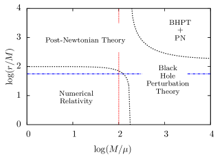
Figure 1: Regions of binary parameter space in which different formalisms apply. Post-Newtonian (PN) approximation applies best to binaries with wide orbital separation (or equivalently low frequency). Black hole perturbation (BHP) theory is relevant for binaries with small mass ratio $\mu/M$. Numerical relativity (NR) works best for close binaries with comparable masses. This paper makes comparisons between PN and BHP results in their region of mutual overlap.

The interest in eccentric orbits stems from astrophysical considerations Amaro-Seoane et al. (2007, 2014) that indicate extreme-mass-ratio inspirals (EMRIs) should be born with high eccentricities. Other work Hopman and Alexander (2005) suggests EMRIs will have a distribution peaked about $e=0.7$ as they enter the eLISA passband. Less extreme (intermediate) mass ratio inspirals (IMRIs) may also exist Miller and Colbert (2004) and might appear as detections in Advanced LIGO Brown et al. (2007); Amaro-Seoane et al. (2007). Whether they exist, and have significant eccentricities, is an issue for observations to settle. The PN expansion for eccentric orbits is known through 3PN relative order Arun et al. (2008a, b, 2009); Blanchet (2014). The present paper confirms the accuracy of that expansion for the energy flux and determines PN eccentricity-dependent coefficients all the way through 7PN order for multiple orders in an expansion in $e^{2}$. The model is improved by developing an understanding of what eccentricity singular functions to factor out at each PN order. In so doing, we are able to obtain better convergence and the ability to compute the flux even as $e\rightarrow 1$. The review by Sasaki and Tagoshi Sasaki and Tagoshi (2003) summarized earlier work on fluxes from slightly eccentric orbits (through $e^{2}$) and more recently results have been obtained Sago and Fujita (2015) on fluxes to $e^{6}$ for 3.5PN and 4PN order.

Our work makes use of the analytic function expansion formalism developed by Mano, Suzuki, and Takasugi (MST) Mano et al. (1996a, b) with a code written in Mathematica (to take advantage of arbitrary precision functions). The MST formalism expands solutions to the Teukolsky equation in infinite series of hypergeometric functions. We convert from solutions to the Teukolsky equation to solutions of the Regge-Wheeler-Zerilli equations and use techniques found in Hopper and Evans (2010); Hopper et al. (2015). Our use of MST is similar to that found in Shah, Friedman, and Whiting Shah et al. (2014), who studied conservative effects, and Shah Shah (2014a), who examined fluxes for circular equatorial orbits on Kerr.

This paper is organized as follows. Those readers interested primarily in new PN results will find them in Secs. IV, V, and VI. Sec. IV contains original work in calculating the 1.5PN, 2.5PN, and 3PN hereditary terms to exceedingly high order in powers of the eccentricity to facilitate comparisons with perturbation theory. It includes a subsection, Sec. IV.3, that uses an asymptotic analysis to guide an understanding of different eccentricity singular factors that appear in the flux at all PN orders. In Sec. V we verify all previously known PN coefficients (i.e., those through 3PN relative order) in the energy flux from eccentric binaries at lowest order in the mass ratio. Sec. VI and App. C present our new findings on PN coefficients in the energy flux from eccentric orbits between 3.5PN and 7PN order. For those interested in the method, Sec. II reviews the MST formalism for analytic function expansions of homogeneous solutions, and describes the conversion from Teukolsky modes to normalized Regge-Wheeler-Zerilli modes. Section III outlines the now-standard procedure of solving the RWZ source problem with extended homogeneous solutions, though now with the added technique of spectral source integration Hopper et al. (2015). Some details on our numerical procedure, which allows calculations to better than 200 decimal places of accuracy, are given in Sec. V.1. Our conclusions are drawn in Sec. VII.

Throughout this paper we set $c=G=1$, and use metric signature $(-+++)$ and sign conventions of Misner, Thorne, and Wheeler Misner et al. (1973). Our notation for the RWZ formalism is that of Hopper and Evans (2010), which derives from earlier work of Martel and Poisson Martel and Poisson (2005).

II Analytic expansions for homogeneous solutions

This section briefly outlines the MST formalism Mano et al. (1996b) (see the detailed review by Sasaki and Tagoshi Sasaki and Tagoshi (2003)) and describes our conversion to analytic expansions for normalized RWZ modes.

II.1 The Teukolsky formalism

The MST approach provides analytic function expansions for general perturbations of a Kerr black hole. With other future uses in mind, elements of our code are based on the general MST expansion. However, the present application is focused solely on eccentric motion in a Schwarzschild background and thus in our discussion below we simply adopt the $a=0$ limit on black hole spin from the outset. The MST method describes gravitational perturbations in the Teukolsky formalism Teukolsky (1973) using the Newman-Penrose scalar $\psi_{4}=-C_{\alpha\beta\gamma\delta}n^{\alpha}\bar{m}^{\beta}n^{\gamma}\bar{m}^{\delta}$ Newman and Penrose (1962, 1963). Here $C_{\alpha\beta\gamma\delta}$ is the Weyl tensor, and its projection is made on elements of the Kinnersley null tetrad (see Kinnersley (1969); Teukolsky (1973) for its components).

In our application the line element is

$$ds^{2}=-fdt^{2}+f^{-1}dr^{2}+r^{2}\left(d\theta^{2}+\sin^{2}\theta\,d\varphi^{2}\right),$$ (1)

as written in Schwarzschild coordinates, with $f(r)=1-2M/r$. The Teukolsky equation Teukolsky (1973) with spin-weight $s=-2$ is satisfied (when $a=0$) by $r^{4}\psi_{4}$, with $\psi_{4}$ separated into Fourier-harmonic modes by

$$\psi_{4}=r^{-4}\sum_{lm}\,\int\,d\omega\,e^{-i\omega t}\,R_{lm\omega}(r)\,{}_{-2}Y_{lm}(\theta,\varphi).$$ (2)

Here ${}_{s}Y_{lm}$ are spin-weighted spherical harmonics. The Teukolsky equation for $R_{lm\omega}$ reduces in our case to the Bardeen-Press equation Bardeen and Press (1973); Cutler et al. (1994), which away from the source has the homogeneous form

$$\left[r^{2}f\frac{d^{2}}{dr^{2}}-2(r-M)\frac{d}{dr}+U_{l\omega}(r)\right]\,R_{lm\omega}(r)=0,$$ (3)

with potential

$$U_{l\omega}(r)=\frac{1}{f}\left[\omega^{2}r^{2}-4i\omega(r-3M)\right]-(l-1)(l+2).$$ (4)

Two independent homogeneous solutions are of interest, which have, respectively, causal behavior at the horizon, $R^{\rm in}_{lm\omega}$, and at infinity, $R^{\rm up}_{lm\omega}$,

$$R^{\rm in}_{lm\omega} =\begin{cases}B^{\rm trans}_{lm\omega}r^{2}f\,e^{-i\omega r_{*}}\,&r\rightarrow 2M\\ B^{\rm ref}_{lm\omega}r^{3}\,e^{i\omega r_{*}}+\frac{B^{\rm in}_{lm\omega}}{r}\,e^{-i\omega r_{*}}\,&r\rightarrow+\infty,\end{cases}$$ (5)

$$R^{\rm up}_{lm\omega} =\begin{cases}C^{\rm up}_{lm\omega}\,e^{i\omega r_{*}}+C^{\rm ref}_{lm\omega}r^{2}f\,e^{-i\omega r_{*}}\,&r\rightarrow 2M\\ C^{\rm trans}_{lm\omega}r^{3}\,e^{i\omega r_{*}}\,&r\rightarrow+\infty,\end{cases}$$ (6)

where $B$ and $C$ are used for incident, reflected, and transmitted amplitudes. Here $r_{*}$ is the usual Schwarzschild tortoise coordinate $r_{*}=r+2M\log(r/2M-1)$.

II.2 MST analytic function expansions for $R_{lm\omega}$

The MST formalism makes separate analytic function expansions for the solutions near the horizon and near infinity. We begin with the near-horizon solution.

II.2.1 Near-horizon (inner) expansion

After factoring out terms that arise from the existence of singular points, $R^{\rm in}_{lm\omega}$ is represented by an infinite series in hypergeometric functions

$$R_{lm\omega}^{\text{in}} =e^{i\epsilon x}(-x)^{2-i\epsilon}p_{\text{in}}^{\nu}(x),$$ (7)

$$p_{\text{in}}^{\nu}(x) =\sum_{n=-\infty}^{\infty}a_{n}p_{n+\nu}(x),$$ (8)

where $\epsilon=2M\omega$ and $x=1-r/2M$. The functions $p_{n+\nu}(x)$ are an alternate notation for the hypergeometric functions ${}_{2}F_{1}(a,b;c;x)$, with the arguments in this case being

$$p_{n+\nu}(x)={}_{2}F_{1}(n+\nu+1-i\epsilon,-n-\nu-i\epsilon;3-2i\epsilon;x).$$ (9)

The parameter $\nu$ is freely specifiable and referred to as the renormalized angular momentum, a generalization of $l$ to non-integer (and sometimes complex) values.

The series coefficients $a_{n}$ satisfy a three-term recurrence relation

$$\alpha_{n}^{\nu}a_{n+1}+\beta_{n}^{\nu}a_{n}+\gamma_{n}^{\nu}a_{n-1}=0,$$ (10)

where $\alpha_{n}^{\nu}$, $\beta_{n}^{\nu}$, and $\gamma_{n}^{\nu}$ depend on $\nu$, $l$, $m$, and $\epsilon$ (see App. B and Refs. Mano et al. (1996b) and Sasaki and Tagoshi (2003) for details). The recurrence relation has two linearly-independent solutions, $a_{n}^{(1)}$ and $a_{n}^{(2)}$. Other pairs of solutions, say $a_{n}^{(1^{\prime})}$ and $a_{n}^{(2^{\prime})}$, can be obtained by linear transformation. Given the asymptotic form of $\alpha_{n}^{\nu}$, $\beta_{n}^{\nu}$, and $\gamma_{n}^{\nu}$, it is possible to find pairs of solutions such that $\lim_{n\rightarrow+\infty}a_{n}^{(1)}/a_{n}^{(2)}=0$ and $\lim_{n\rightarrow-\infty}a_{n}^{(1^{\prime})}/a_{n}^{(2^{\prime})}=0$. The two sequences $a_{n}^{(1)}$ and $a_{n}^{(1^{\prime})}$ are called minimal solutions (while $a_{n}^{(2)}$ and $a_{n}^{(2^{\prime})}$ are dominant solutions), but in general the two sequences will not coincide. This is where the free parameter $\nu$ comes in. It turns out possible to choose $\nu$ such that a unique minimal solution emerges (up to a multiplicative constant), with $a_{n}(\nu)$ uniformly valid for $-\infty<n<\infty$ and with the series converging. The procedure for finding $\nu$, which depends on frequency, and then finding $a_{n}(\nu)$, involves iteratively solving for the root of an equation that contains continued fractions and resolving continued fraction equations. We give details in App. B, but refer the reader to Sasaki and Tagoshi (2003) for a complete discussion. The expansion for $R_{lm\omega}^{\rm in}$ converges everywhere except $r=\infty$. For the behavior there we need a separate expansion.

II.2.2 Near-infinity (outer) expansion

After again factoring out terms associated with singular points, an infinite expansion can be written Mano et al. (1996b); Sasaki and Tagoshi (2003); Leaver (1986) for the outer solution $R^{\rm up}_{lm\omega}$ with outgoing wave dependence,

$$R^{\rm up}_{lm\omega} =2^{\nu}e^{-\pi\epsilon}e^{-i\pi(\nu-1)}e^{iz}z^{\nu+i\epsilon}(z-\epsilon)^{2-i\epsilon}$$ (11)

$$\times\sum_{n=-\infty}^{\infty}i^{n}\frac{(\nu-1-i\epsilon)_{n}}{(\nu+3+i\epsilon)_{n}}b_{n}(2z)^{n}$$

$$\qquad\qquad\times\Psi(n+\nu-1-i\epsilon,2n+2\nu+2;-2iz).$$

Here $z=\omega r=\epsilon(1-x)$ is another dimensionless variable, $(\zeta)_{n}=\Gamma(\zeta+n)/\Gamma(\zeta)$ is the (rising) Pochhammer symbol, and $\Psi(a,c;x)$ are irregular confluent hypergeometric functions. The free parameter $\nu$ has been introduced again as well. The limiting behavior $\lim_{|x|\rightarrow\infty}\Psi(a,c;x)\rightarrow x^{-a}$ guarantees the proper asymptotic dependence $R^{\rm up}_{lm\omega}=C^{\rm trans}_{lm\omega}(z/\omega)^{3}\,e^{i(z+\epsilon\log{z})}$.

Substituting the expansion in (3) produces a three-term recurrence relation for $b_{n}$. Remarkably, because of the Pochhammer symbol factors that were introduced in (11), the recurrence relation for $b_{n}$ is identical to the previous one (10) for the inner solution. Thus the same value for the renormalized angular momentum $\nu$ provides a uniform minimal solution for $b_{n}$, which can be identified with $a_{n}$ up to an arbitrary choice of normalization.

II.2.3 Recurrence relations for homogeneous solutions

Both the ordinary hypergeometric functions ${}_{2}F_{1}(a,b;c;z)$ and the irregular confluent hypergeometric functions $\Psi(a,b;z)$ admit three term recurrence relations, which can be used to speed the construction of solutions Shah (2014b). The hypergeometric functions $p_{n+\nu}$ in the inner solution (8) satisfy

$$p_{n+\nu}=-\frac{2n+2\nu-1}{(n+\nu-1)(2+n+\nu-i\epsilon)(n+\nu-i\epsilon)}$$

$$\hskip 12.91663pt\times\left[(n+\nu)(n+\nu-1)(2x-1)+(2i+\epsilon)\epsilon\right]p_{n+\nu-1}$$

$$\hskip 12.91663pt-\frac{(n+\nu)(n+\nu+i\epsilon-3)(n+\nu+i\epsilon-1)}{(n+\nu-1)(2+n+\nu-i\epsilon)(n+\nu-i\epsilon)}p_{n+\nu-2}.$$

Defining by analogy with Eqn. (9)

$$q_{n+\nu}\equiv\Psi(n+\nu-i\epsilon-1,2n+2\nu+2;-2iz),$$ (13)

the irregular confluent hypergeometric functions satisfy

$$q_{n+\nu}=\frac{(2n+2\nu-1)}{(n+\nu-1)(n+\nu-i\epsilon-2)z^{2}}$$

$$\hskip 12.91663pt\times\left[2n^{2}+2\nu(\nu-1)+n(4\nu-2)-(2+i\epsilon)z\right]q_{n+\nu-1}$$

$$\hskip 12.91663pt+\frac{(n+\nu)(1+n+\nu+i\epsilon)}{(n+\nu-1)(n+\nu-i\epsilon-2)z^{2}}q_{n+\nu-2}.$$ (14)

II.3 Mapping to RWZ master functions

In this work we map the analytic function expansions of $R_{lm\omega}$ to ones for the RWZ master functions. The reason stems from having pre-existing coding infrastructure for solving RWZ problems Hopper and Evans (2010) and the ease in reading off gravitational wave fluxes. The Detweiler-Chandrasekhar transformation Chandrasekhar (1975); Chandrasekhar and Detweiler (1975); Chandrasekhar (1983) maps $R_{lm\omega}$ to a solution $X^{\rm RW}_{lm\omega}$ of the Regge-Wheeler equation via

$$X^{\rm RW}_{lm\omega}=r^{3}\left(\frac{d}{dr}-\frac{i\omega}{f}\right)\left(\frac{d}{dr}-\frac{i\omega}{f}\right)\frac{R_{lm\omega}}{r^{2}}.$$ (15)

For odd parity ($l+m=$ odd) this completes the transformation. For even parity, we make a second transformation Berndston (2007) to map through to a solution $X_{lm\omega}^{Z}$ of the Zerilli equation

$$X_{lm\omega}^{Z,\pm} =\frac{1}{\lambda(\lambda+1)\pm 3i\omega M}\Bigg{\{}3Mf\frac{dX_{lm\omega}^{\rm{RW},\pm}}{dr}$$ (16)

$$\hskip 30.1388pt+\left[\lambda(\lambda+1)+\frac{9M^{2}f}{r(\lambda r+3M)}\right]X_{lm\omega}^{\rm{RW},\pm}\Bigg{\}}.$$

Here $\lambda=(l-1)(l+2)/2$. We have introduced above the $\pm$ notation to distinguish outer ($+$) and inner ($-$) solutions–a notation that will be used further in Sec. III.2. [When unambiguous we often use $X_{lm\omega}$ to indicate either the RW function (with $l+m=$ odd) or Zerilli function (with $l+m=$ even).] The RWZ functions satisfy the homogeneous form of (34) below with their respective parity-dependent potentials $V_{l}$.

The normalization of $R_{lm\omega}$ in the MST formalism is set by adopting some starting value, say $a_{0}=1$, in solving the recurrence relation for $a_{n}$. This guarantees that the RWZ functions will not be unit-normalized at infinity or on the horizon, but instead will have some $A^{\pm}_{lm\omega}$ such that $X^{\pm}_{lm\omega}\sim A^{\pm}_{lm\omega}\,e^{\pm i\omega r_{*}}$. We find it advantageous though to construct unit-normalized modes $\hat{X}^{\pm}_{lm\omega}\sim\exp(\pm i\omega r_{*})$ Hopper and Evans (2010). To do so we first determine the initial amplitudes $A^{\pm}_{lm\omega}$ by passing the MST expansions in Eqns. (7), (8), and (11) through the transformation in Eqns. (15) (and additionally (16) as required) to find

$$\begin{split}A_{lm\omega}^{\text{RW},+}&=-2^{-1+4iM\omega}i\omega(M\omega)^{2iM\omega}e^{-\pi M\omega-\frac{1}{2}i\pi\nu}\\ &\times\sum_{n=-\infty}^{\infty}(-1)^{n}\bigg{\{}(\nu-1)\nu(\nu+1)(\nu+2)+4iM\left[2\nu(\nu+1)-7\right]\omega+32iM^{3}\omega^{3}+400M^{4}\omega^{4}\\ &\hskip 43.05542pt+20M^{2}\left[2\nu(\nu+1)-1\right]\omega^{2}+2(2\nu+1)\Big{[}4M\omega(5M\omega+i)+\nu(\nu+1)-1\Big{]}n\\ &\hskip 43.05542pt+\Big{[}8M\omega(5M\omega+i)+6\nu(\nu+1)-1\Big{]}n^{2}+(4\nu+2)n^{3}+n^{4}\bigg{\}}\frac{(\nu-2iM\omega-1)_{n}}{(\nu+2iM\omega+3)_{n}}a_{n},\end{split}$$ (17)

$$\begin{split}A_{lm\omega}^{Z,+}&=-\frac{2^{-1+4iM\omega}i\omega(M\omega)^{2iM\omega}\left[(l-1)l(l+1)(l+2)+12iM\omega\right]}{(l-1)l(l+1)(l+2)-12iM\omega}\\ &\times\sum_{n=-\infty}^{\infty}e^{\frac{1}{2}i\pi(2iM\omega+2n-\nu)}\Big{[}2M\omega(7i-6M\omega)+n(n+2\nu+1)+\nu(\nu+1)\Big{]}\\ &\hskip 43.05542pt\times\Big{\{}-2\left[1+3M\omega(2M\omega+i)\right]+n(n+2\nu+1)+\nu(\nu+1)\Big{\}}\frac{(\nu-2iM\omega-1)_{n}}{(\nu+2iM\omega+3)_{n}}a_{n}.\end{split}$$ (18)

$$\begin{split}&A_{lm\omega}^{\text{RW},-}=A_{lm\omega}^{Z,-}=-\frac{1}{M}e^{2iM\omega}(2M\omega+i)(4M\omega+i)\sum_{n=-\infty}^{\infty}a_{n},\end{split}$$ (19)

These amplitudes are then used to renormalize the initial $a_{n}$.

III Solution to the perturbation equations using MST and SSI

We briefly review here the procedure for solving the perturbation equations for eccentric orbits on a Schwarzschild background using MST and a recently developed spectral source integration (SSI) Hopper et al. (2015) scheme, both of which are needed for high accuracy calculations.

III.1 Bound orbits on a Schwarzschild background

We consider generic bound motion between a small mass $\mu$, treated as a point particle, and a Schwarzschild black hole of mass $M$, with $\mu/M\ll 1$. Schwarzschild coordinates $x^{\mu}=(t,r,\theta,\varphi)$ are used. The trajectory of the particle is given by $x_{p}^{\alpha}(\tau)=\left[t_{p}(\tau),r_{p}(\tau),\pi/2,\varphi_{p}(\tau)\right]$ in terms of proper time $\tau$ (or some other suitable curve parameter) and the motion is assumed, without loss of generality, to be confined to the equatorial plane. Throughout this paper, a subscript $p$ denotes evaluation at the particle location. The four-velocity is $u^{\alpha}=dx_{p}^{\alpha}/d\tau$.

At zeroth order the motion is geodesic in the static background and the equations of motion have as constants the specific energy $\mathcal{E}=-u_{t}$ and specific angular momentum $\mathcal{L}=u_{\varphi}$. The four-velocity becomes

$$u^{\alpha}=\left(\frac{{\mathcal{E}}}{f_{p}},u^{r},0,\frac{{\mathcal{L}}}{r_{p}^{2}}\right).$$ (20)

The constraint on the four-velocity leads to

$$\dot{r}_{p}^{2}(t)=f_{p}^{2}\left[1-\frac{f_{p}}{{\mathcal{E}}^{2}}\left(1+\frac{{\mathcal{L}}^{2}}{r^{2}}\right)\right],$$ (21)

where dot is the derivative with respect to $t$. Bound orbits have ${\mathcal{E}}<1$ and, to have two turning points, must at least have ${\mathcal{L}}>2\sqrt{3}M$. In this case, the pericentric radius, $r_{\rm min}$, and apocentric radius, $r_{\rm max}$, serve as alternative parameters to ${\mathcal{E}}$ and ${\mathcal{L}}$, and also give rise to definitions of the (dimensionless) semi-latus rectum $p$ and the eccentricity $e$ (see Cutler et al. (1994); Barack and Sago (2010)). These various parameters are related by

$${\mathcal{E}}^{2}=\frac{(p-2)^{2}-4e^{2}}{p(p-3-e^{2})},\quad{\mathcal{L}}^{2}=\frac{p^{2}M^{2}}{p-3-e^{2}},$$ (22)

and $r_{\rm max}=pM/(1-e)$ and $r_{\rm min}=pM/(1+e)$. The requirement of two turning points also sets another inequality, $p>6+2e$, with the boundary $p=6+2e$ of these innermost stable orbits being the separatrix Cutler et al. (1994).

Integration of the orbit is described in terms of an alternate curve parameter, the relativistic anomaly $\chi$, that gives the radial position a Keplerian-appearing form Darwin (1959)

$$r_{p}\left(\chi\right)=\frac{pM}{1+e\cos\chi}.$$ (23)

One radial libration makes a change $\Delta\chi=2\pi$. The orbital equations then have the form

$$\frac{dt_{p}}{d\chi} =\frac{r_{p}\left(\chi\right)^{2}}{M(p-2-2e\cos\chi)}\left[\frac{(p-2)^{2}-4e^{2}}{p-6-2e\cos\chi}\right]^{1/2},$$

$$\frac{d\varphi_{p}}{d\chi} =\left[\frac{p}{p-6-2e\cos\chi}\right]^{1/2},$$ (24)

$$\frac{d\tau_{p}}{d\chi} =\frac{Mp^{3/2}}{(1+e\cos\chi)^{2}}\left[\frac{p-3-e^{2}}{p-6-2e\cos\chi}\right]^{1/2},$$

and $\chi$ serves to remove singularities in the differential equations at the radial turning points Cutler et al. (1994). Integrating the first of these equations provides the fundamental frequency and period of radial motion

$$\Omega_{r}\equiv\frac{2\pi}{T_{r}},\quad\quad T_{r}\equiv\int_{0}^{2\pi}\left(\frac{dt_{p}}{d\chi}\right)d\chi.$$ (25)

There is an analytic solution to the second equation for the azimuthal advance, which is especially useful in our present application,

$$\varphi_{p}(\chi)=\left(\frac{4p}{p-6-2e}\right)^{1/2}\,F\left(\frac{\chi}{2}\,\middle|\,-\frac{4e}{p-6-2e}\right).$$ (26)

Here $F(x|m)$ is the incomplete elliptic integral of the first kind Gradshteyn et al. (2007). The average of the angular frequency $d\varphi_{p}/dt$ is found by integrating over a complete radial oscillation

$$\Omega_{\varphi}=\frac{4}{T_{r}}\left(\frac{p}{p-6-2e}\right)^{1/2}\,K\left(-\frac{4e}{p-6-2e}\right),$$ (27)

where $K(m)$ is the complete elliptic integral of the first kind Gradshteyn et al. (2007). Relativistic orbits will have $\Omega_{r}\neq\Omega_{\varphi}$, but with the two approaching each other in the Newtonian limit.

III.2 Solutions to the TD master equation

This paper draws upon previous work Hopper and Evans (2010) in solving the RWZ equations, though here we solve the homogeneous equations using the MST analytic function expansions discussed in Sec. II. A goal is to find solutions to the inhomogeneous time domain (TD) master equations

$$\left[-\frac{\partial^{2}}{\partial t^{2}}+\frac{\partial^{2}}{\partial r_{*}^{2}}-V_{l}(r)\right]\Psi_{lm}(t,r)=S_{lm}(t,r).$$ (28)

The parity-dependent source terms $S_{lm}$ arise from decomposing the stress-energy tensor of a point particle in spherical harmonics. They are found to take the form

$$S_{lm}=G_{lm}(t)\,\delta[r-r_{p}(t)]+F_{lm}(t)\,\delta^{\prime}[r-r_{p}(t)],$$ (29)

where $G_{lm}(t)$ are $F_{lm}(t)$ are smooth functions. Because of the periodic radial motion, both $\Psi_{lm}$ and $S_{lm}$ can be written as Fourier series

$$\Psi_{lm}(t,r) =\sum_{n=-\infty}^{\infty}X_{lmn}(r)\,e^{-i\omega t},$$ (30)

$$S_{lm}(t,r) =\sum_{n=-\infty}^{\infty}Z_{lmn}(r)\,e^{-i\omega t},$$ (31)

where the $\omega\equiv\omega_{mn}=m\Omega_{\varphi}+n\Omega_{r}$ reflects the bi-periodicity of the source motion. The inverses are

$$X_{lmn}(r) =\frac{1}{T_{r}}\int_{0}^{T_{r}}dt\ \Psi_{lm}(t,r)\,e^{i\omega t},$$ (32)

$$Z_{lmn}(r) =\frac{1}{T_{r}}\int_{0}^{T_{r}}dt\ S_{lm}(t,r)\,e^{i\omega t}.$$ (33)

Inserting these series in Eqn. (28) reduces the TD master equation to a set of inhomogeneous ordinary differential equations (ODEs) tagged additionally by harmonic $n$,

$$\left[\frac{d^{2}}{dr_{*}^{2}}+\omega^{2}-V_{l}(r)\right]X_{lmn}(r)=Z_{lmn}(r).$$ (34)

The homogeneous version of this equation is solved by MST expansions. The unit normalized solutions at infinity (up) are $\hat{X}^{+}_{lmn}$ while the horizon-side (in) solutions are $\hat{X}^{-}_{lmn}$. These independent solutions provide a Green function, from which the particular solution to Eqn. (34) is derived

$$X_{lmn}(r)=c^{+}_{lmn}(r)\,\hat{X}^{+}_{lmn}(r)+c^{-}_{lmn}(r)\,\hat{X}^{-}_{lmn}(r).$$ (35)

See Ref. Hopper and Evans (2010) for further details. However, Gibbs behavior in the Fourier series makes reconstruction of $\Psi_{lm}$ in this fashion problematic. Instead, the now standard approach is to derive the TD solution using the method of extended homogeneous solutions (EHS) Barack et al. (2008).

We form first the frequency domain (FD) EHS

$$X^{\pm}_{lmn}(r)\equiv C^{\pm}_{lmn}\hat{X}_{lmn}^{\pm}(r),\quad\quad r>2M,$$ (36)

where the normalization coefficients, $C^{+}_{lmn}=c^{+}_{lmn}(r_{\rm max})$ and $C^{-}_{lmn}=c^{-}_{lmn}(r_{\rm min})$, are discussed in the next subsection. From these solutions we define the TD EHS,

$$\Psi^{\pm}_{lm}(t,r)\equiv\sum_{n}X^{\pm}_{lmn}(r)\,e^{-i\omega t},\quad\quad r>2M.$$ (37)

Then the particular solution to Eqn. (28) is formed by abutting the two TD EHS at the particle’s location,

$$\begin{split}\Psi_{lm}(t,r)&=\Psi^{+}_{lm}(t,r)\theta\left[r-r_{p}(t)\right]\\ &\hskip 43.05542pt+\Psi^{-}_{lm}(t,r)\theta\left[r_{p}(t)-r\right].\end{split}$$ (38)

III.3 Normalization coefficients

The following integral must be evaluated to obtain the normalization coefficients $C^{\pm}_{lmn}$ Hopper and Evans (2010)

$$C_{lmn}^{\pm} =\frac{1}{W_{lmn}T_{r}}\int_{0}^{T_{r}}\Bigg{[}\frac{1}{f_{p}}\hat{X}^{\mp}_{lmn}G_{lm}\hskip 21.52771pt$$ (39)

$$\hskip 21.52771pt+\left(\frac{2M}{r_{p}^{2}f_{p}^{2}}\hat{X}^{\mp}_{lmn}-\frac{1}{f_{p}}\frac{d\hat{X}^{\mp}_{lmn}}{dr}\right)F_{lm}\Bigg{]}e^{i\omega t}\,dt,$$

where $W_{lmn}$ is the Wronskian

$$W_{lmn}=f\hat{X}^{-}_{lmn}\frac{d\hat{X}^{+}_{lmn}}{dr}-f\hat{X}^{+}_{lmn}\frac{d\hat{X}^{-}_{lmn}}{dr}.$$ (40)

The integral in (39) is often computed using Runge-Kutta (or similar) numerical integration, which is algebraically convergent. As shown in Hopper et al. (2015) when MST expansions are used with arbitrary-precision algorithms to obtain high numerical accuracy (i.e., much higher than double precision), algebraically-convergent integration becomes prohibitively expensive. We recently developed the SSI scheme, which provides exponentially convergent source integrations, in order to make possible MST calculations of eccentric-orbit EMRIs with arbitrary precision. In the present paper our calculations of energy fluxes have up to 200 decimal places of accuracy.

The central idea is that, since the source terms $G_{lm}(t)$ and $F_{lm}(t)$ and the modes $X^{\pm}_{lmn}(r)$ are smooth functions, the integrand in (39) can be replaced by a sum over equally-spaced samples

$$C^{\pm}_{lmn}=\frac{1}{NW_{lmn}}\sum_{k=0}^{N-1}\bar{E}^{\pm}_{lmn}(t_{k})\,e^{in\Omega_{r}t_{k}}.$$ (41)

In this expression $\bar{E}_{lmn}$ is the following $T_{r}$-periodic smooth function of time

$$\bar{E}^{\pm}_{lmn}(t)=\frac{\bar{G}_{lm}(t)}{f_{p}}\,\hat{X}^{\mp}_{lmn}(r_{p}(t))$$ (42)

$$\hskip 21.52771pt+\frac{2M}{r_{p}^{2}}\frac{\bar{F}_{lm}(t)}{f_{p}^{2}}\,\hat{X}^{\mp}_{lmn}(r_{p}(t))-\frac{\bar{F}_{lm}(t)}{f_{p}}\,\partial_{r}\hat{X}^{\mp}_{lmn}(r_{p}(t)).$$

It is evaluated at $N$ times that are evenly spaced between $0$ and $T_{r}$, i.e., $t_{k}\equiv kT_{r}/N$. In this expression $\bar{G}_{lm}$ is related to the term in Eqn. (29) by $\bar{G}_{lm}=G_{lm}e^{im\Omega_{\varphi}t}$ (likewise for $\bar{F}_{lm}$). It is then found that the sum in (41) exponentially converges to the integral in (39) as the sample size $N$ increases.

One further improvement was found. The curve parameter in (39) can be arbitrarily changed and the sum (41) is thus replaced by one with even sampling in the new parameter. Switching from $t$ to $\chi$ has the effect of smoothing out the source motion, and as a result the sum

$$C^{\pm}_{lmn} =\frac{\Omega_{r}}{NW_{lmn}}\sum_{k}\frac{dt_{p}}{d\chi}\bar{E}^{\pm}_{lmn}(t_{k})\,e^{in\Omega_{r}t_{k}},$$ (43)

evenly sampled in $\chi$ ($\chi_{k}=2\pi k/N$ with $t_{k}=t_{p}(\chi_{k})$) converges at a substantially faster rate. This is particularly advantageous for computing normalizations for high eccentricity orbits.

Once the $C^{\pm}_{lmn}$ are determined, the energy fluxes at infinity can be calculated using

$$\left\langle\frac{dE}{dt}\right\rangle=\sum_{lmn}\frac{\omega^{2}}{64\pi}\frac{(l+2)!}{(l-2)!}|C^{+}_{lmn}|^{2},$$ (44)

given our initial unit normalization of the modes $\hat{X}_{lmn}^{\pm}$. We return to this subject and specific algorithmic details in Sec. V.1.

IV Preparing the PN expansion for comparison with perturbation theory

The formalism we briefly discussed in the preceding sections, along with the technique in Hopper et al. (2015), was used to build a code for computing energy fluxes at infinity from eccentric orbits to accuracies as high as 200 decimal places, and to then confirm previous work in PN theory and to discover new high PN order terms. In this section we make further preparation for that comparison with PN theory. The average energy and angular momentum fluxes from an eccentric binary are known to 3PN relative order Arun et al. (2008a, b, 2009) (see also the review by Blanchet Blanchet (2014)). The expressions are given in terms of three parameters; e.g., the gauge-invariant post-Newtonian compactness parameter $x\equiv\left[(m_{1}+m_{2})\Omega_{\varphi}\right]^{2/3}$, the eccentricity, and the symmetric mass ratio $\nu=m_{1}m_{2}/(m_{1}+m_{2})^{2}\simeq\mu/M$ (not to be confused with our earlier use of $\nu$ for renormalized angular momentum parameter). In this paper we ignore contributions to the flux that are higher order in the mass ratio than $\mathcal{O}(\nu^{2})$, as these would require a second-order GSF calculation to reach. The more appropriate compactness parameter in the extreme mass ratio limit is $y\equiv\left(M\Omega_{\varphi}\right)^{2/3}$, with $y=x(1+m_{1}/m_{2})^{-2/3}$ Blanchet (2014). Composed of a set of eccentricity-dependent coefficients, the energy flux through 3PN order has the form

$$\mathcal{F}_{\rm 3PN}=\left\langle\frac{dE}{dt}\right\rangle_{\rm 3PN}=\frac{32}{5}\left(\frac{\mu}{M}\right)^{2}y^{5}\,\Bigl{(}\mathcal{I}_{0}+y\,\mathcal{I}_{1}+y^{3/2}\,\mathcal{K}_{3/2}+y^{2}\,\mathcal{I}_{2}+y^{5/2}\,\mathcal{K}_{5/2}+y^{3}\,\mathcal{I}_{3}+y^{3}\,\mathcal{K}_{3}\Bigr{)}.$$ (45)

The $\mathcal{I}_{n}$ are instantaneous flux functions [of eccentricity and (potentially) $\log(y)$] that have known closed-form expressions (summarized below). The $\mathcal{K}_{n}$ coefficients are hereditary, or tail, contributions (without apparently closed forms). The purpose of this section is to derive new expansions for these hereditary terms and to understand more generally the structure of all of the eccentricity dependent coefficients, up to 3PN order and beyond.

IV.1 Known instantaneous energy flux terms

For later reference and use, we list here the instantaneous energy flux functions, expressed in modified harmonic (MH) gauge Arun et al. (2008a, 2009); Blanchet (2014) and in terms of $e_{t}$, a particular definition of eccentricity (time eccentricity) used in the quasi-Keplerian (QK) representation Damour (1985) of the orbit (see also Königsdörffer and Gopakumar (2005, 2006); Arun et al. (2008a, b, 2009); Gopakumar and Schäfer (2011); Blanchet (2014))

$$\mathcal{I}_{0} =\frac{1}{(1-e_{t}^{2})^{7/2}}{\left(1+\frac{73}{24}~{}e_{t}^{2}+\frac{37}{96}~{}e_{t}^{4}\right)},$$ (46)

$$\mathcal{I}_{1} =\frac{1}{(1-e_{t}^{2})^{9/2}}{\left(-\frac{1247}{336}+\frac{10475}{672}e_{t}^{2}+\frac{10043}{384}e_{t}^{4}+\frac{2179}{1792}e_{t}^{6}\right)},$$ (47)

$$\begin{split}\mathcal{I}_{2}&=\frac{1}{(1-e_{t}^{2})^{11/2}}{\left(-\frac{203471}{9072}-\frac{3807197}{18144}e_{t}^{2}-\frac{268447}{24192}e_{t}^{4}+\frac{1307105}{16128}e_{t}^{6}+\frac{86567}{64512}e_{t}^{8}\right)}\\ &\hskip 215.2771pt+\frac{1}{(1-e_{t}^{2})^{5}}\left(\frac{35}{2}+\frac{6425}{48}e_{t}^{2}+\frac{5065}{64}e_{t}^{4}+\frac{185}{96}e_{t}^{6}\right),\end{split}$$ (48)

$$\begin{split}\mathcal{I}_{3}&=\frac{1}{(1-e_{t}^{2})^{13/2}}\left(\frac{2193295679}{9979200}+\frac{20506331429}{19958400}e_{t}^{2}-\frac{3611354071}{13305600}e_{t}^{4}\right.\\ \biggl{.}&\hskip 193.74939pt+\frac{4786812253}{26611200}e_{t}^{6}+\frac{21505140101}{141926400}e_{t}^{8}-\frac{8977637}{11354112}e_{t}^{10}\biggr{)}\\ &+\frac{1}{(1-e_{t}^{2})^{6}}\left(-\frac{14047483}{151200}+\frac{36863231}{100800}e_{t}^{2}+\frac{759524951}{403200}e_{t}^{4}+\frac{1399661203}{2419200}e_{t}^{6}+\frac{185}{48}e_{t}^{8}\right)\\ &+\frac{1712}{105}\log\left[\frac{y}{y_{0}}\frac{1+\sqrt{1-e_{t}^{2}}}{2(1-e_{t}^{2})}\right]F(e_{t}),\end{split}$$ (49)

where the function $F(e_{t})$ in Eqn. (49) has the following closed-form Arun et al. (2008a)

$$F(e_{t})=\frac{1}{(1-e_{t}^{2})^{13/2}}\bigg{(}1+\frac{85}{6}e_{t}^{2}+\frac{5171}{192}e_{t}^{4}+\frac{1751}{192}e_{t}^{6}+\frac{297}{1024}e_{t}^{8}\bigg{)}.$$ (50)

The first flux function, $\mathcal{I}_{0}(e_{t})$, is the enhancement function of Peters and Mathews Peters and Mathews (1963) that arises from quadrupole radiation and is computed using only the Keplerian approximation of the orbital motion. The term “enhancement function” is used for functions like $\mathcal{I}_{0}(e_{t})$ that are defined to limit on unity as the orbit becomes circular (with one exception discussed below). Except for $\mathcal{I}_{0}$, the flux coefficients generally depend upon choice of gauge, compactness parameter, and PN definition of eccentricity. [Note that the extra parameter $y_{0}$ in the $\mathcal{I}_{3}$ log term cancels a corresponding log term in the 3PN hereditary flux. See Eqn. (53) below.] We also point out here the appearance of factors of $1-e_{t}^{2}$ with negative, odd-half-integer powers, which make the PN fluxes diverge as $e_{t}\rightarrow 1$. We will have more to say in what follows about these eccentricity singular factors.

IV.2 Making heads or tails of the hereditary terms

The hereditary contributions to the energy flux can be defined Arun et al. (2008a) in terms of an alternative set of functions

$$\mathcal{K}_{3/2}=4\pi\,\varphi(e_{t}),$$ (51)

$$\mathcal{K}_{5/2}=-\frac{8191}{672}\,\pi\,\psi(e_{t}),$$ (52)

$$\mathcal{K}_{3}=-\frac{1712}{105}\,\chi(e_{t})+\left[-\frac{116761}{3675}+\frac{16}{3}\,\pi^{2}-\frac{1712}{105}\,\gamma_{\text{E}}-\frac{1712}{105}\log\left(\frac{4y^{3/2}}{y_{0}}\right)\right]\,F(e_{t}),$$ (53)

where $\gamma_{\text{E}}$ is the Euler constant and $F$, $\varphi$, $\psi$, and $\chi$ are enhancement functions (though $\chi$ is the aforementioned special case, which instead of limiting on unity vanishes as $e_{t}\rightarrow 0$). (Note also that the enhancement function $\chi(e_{t})$ should not to be confused with the orbital motion parameter $\chi$.) Given the limiting behavior of these new functions, the circular orbit limit becomes obvious. The 1.5PN enhancement function $\varphi$ was first calculated by Blanchet and Schäfer Blanchet and Schafer (1993) following discovery of the circular orbit limit ($4\pi$) of the tail by Wiseman Wiseman (1993) (analytically) and Poisson Poisson (1993) (numerically, in an early BHP calculation). The function $F(e_{t})$, given above in Eqn. (50), is closed form, while $\varphi$, $\psi$, and $\chi$ (apparently) are not. Indeed, the lack of closed-form expressions for $\varphi$, $\psi$, and $\chi$ presented a problem for us. Arun et al. Arun et al. (2008a, b, 2009) computed these functions numerically and plotted them, but gave only low-order expansions in eccentricity. For example Ref. Arun et al. (2009) gives for the 1.5PN tail function

$$\varphi(e_{t})=1+\frac{2335}{192}e_{t}^{2}+\frac{42955}{768}e_{t}^{4}+\cdots.$$ (54)

One of the goals of this paper became finding means of calculating these functions with (near) arbitrary accuracy.

The expressions above are written as functions of the eccentricity $e_{t}$. However, the 1.5PN tail $\varphi$ and the functions $F$ and $\chi$ only depend upon the binary motion, and moments, computed to Newtonian order. Hence, for these functions (as well as $\mathcal{I}_{0}$) there is no distinction between $e_{t}$ and the usual Keplerian eccentricity. Nevertheless, since we will reserve $e$ to denote the relativistic (Darwin) eccentricity, we express everything here in terms of $e_{t}$.

Blanchet and Schäfer Blanchet and Schafer (1993) showed that $\varphi(e_{t})$, like the Peters-Mathews enhancement function $\mathcal{I}_{0}$, is determined by the quadrupole moment as computed at Newtonian order from the Keplerian elliptical motion. Using the Fourier series expansion of the time dependence of a Kepler ellipse Peters and Mathews (1963); Maggiore (2007), $\mathcal{I}_{0}$ can be written in terms of Fourier amplitudes of the quadrupole moment by

$$\mathcal{I}_{0}(e_{t})=\frac{1}{16}\sum_{n=1}^{\infty}n^{6}|\!\mathop{\hat{I}}_{(n)}{}_{\!\!ij}^{\!\!(\mathrm{N})}|^{2}=\sum_{n=1}^{\infty}g(n,e_{t})=f(e_{t})=\frac{1}{(1-e_{t}^{2})^{7/2}}{\left(1+\frac{73}{24}~{}e_{t}^{2}+\frac{37}{96}~{}e_{t}^{4}\right)},$$ (55)

which is the previously mentioned closed form expression. Here, $f(e)$ is the traditional Peters-Mathews function name, which is not to be confused with the metric function $f(r)$. In the expression, ${}_{(n)}\hat{I}_{ij}^{(\mathrm{N})}$ is the $n$th Fourier harmonic of the dimensionless quadrupole moment (see sections III through V of Arun et al. (2008a)). The function $g(n,e_{t})$ that represents the square of the quadrupole moment amplitudes is given by

$$g(n,e_{t}) \equiv\frac{1}{2}n^{2}\bigg{\{}\left[-\frac{4}{e_{t}^{3}}-3e_{t}+\frac{7}{e_{t}}\right]nJ_{n}(ne_{t})J_{n}^{\prime}(ne_{t})+\left[\left(e_{t}^{2}+\frac{1}{e_{t}^{2}}-2\right)n^{2}+\frac{1}{e_{t}^{2}}-1\right]J_{n}^{\prime}(ne_{t})^{2}$$

$$\hskip 172.22168pt+\left[\frac{1}{e_{t}^{4}}-\frac{1}{e_{t}^{2}}+\left(\frac{1}{e_{t}^{4}}-e_{t}^{2}-\frac{3}{e_{t}^{2}}+3\right)n^{2}+\frac{1}{3}\right]J_{n}(ne_{t})^{2}\bigg{\}},$$ (56)

and was derived by Peters and Mathews Peters and Mathews (1963) (though the corrected expression can be found in Blanchet and Schafer (1993) or Maggiore (2007)).

These quadrupole moment amplitudes also determine $F(e_{t})$,

$$F(e_{t})=\frac{1}{4}\sum_{n=1}^{\infty}n^{2}\,g(n,e_{t}),$$ (57)

whose closed form expression is found in (50), and the 1.5PN tail function Blanchet and Schafer (1993), which emerges from a very similar sum

$$\varphi(e_{t})=\sum_{n=1}^{\infty}\frac{n}{2}\,g(n,e_{t}).$$ (58)

Unfortunately, the odd factor of $n$ in this latter sum (and more generally any other odd power of $n$) makes it impossible to translate the sum into an integral in the time domain and blocks the usual route to finding a closed-form expression like $f(e_{t})$ and $F(e_{t})$.

The sum (58) might be computed numerically but it is more convenient to have an expression that can be understood at a glance and be rapidly evaluated. The route we found to such an expression leads to several others. We begin with (IV.2) and expand $g(n,e_{t})$, pulling forward the leading factor and writing the remainder as a Maclaurin series in $e_{t}$

$$g(n,e_{t})=\left(\frac{n}{2}\right)^{2n}e_{t}^{2n-4}\left(\frac{1}{\Gamma(n-1)^{2}}-\frac{(n-1)(n^{2}+4n-2)}{2\,\Gamma(n)^{2}}e_{t}^{2}+\frac{6n^{4}+45n^{3}+18n^{2}-48n+8}{48\,\Gamma(n)^{2}}e_{t}^{4}+\cdots\right).$$ (59)

In a sum over $n$, successive harmonics each contribute a series that starts at a progressively higher power of $e_{t}^{2}$. Inspection further shows that for $n=1$ the $e_{t}^{-2}$ and $e_{t}^{0}$ terms vanish, the former because $\Gamma(0)^{-1}\rightarrow 0$. The $n=2$ harmonic is the only one that contributes at $e_{t}^{0}$ [in fact giving $g(2,e_{t})=1$, the circular orbit limit]. The successively higher-order power series in $e_{t}^{2}$ imply that the individual sums that result from expanding (55), (57), and (58) each truncate, with only a finite number of harmonics contributing to the coefficient of any given power of $e_{t}^{2}$.

If we use (59) in (55) and sum, we find $\mathcal{I}_{0}=1+(157/24)e_{t}^{2}+(605/32)e_{t}^{4}+(3815/96)e_{t}^{6}+\cdots$, an infinite series. If on the other hand we introduce the known eccentricity singular factor, take $(1-e_{t}^{2})^{7/2}\,g(n,e_{t})$, re-expand and sum, we then find $1+(73/24)e_{t}^{2}+(37/96)e_{t}^{4}$, the well known Peters-Mathews polynomial term. All the sums for higher-order terms vanish identically. The same occurs if we take a different eccentricity singular factor, expand $(1/4)(1-e_{t}^{2})^{13/2}\,n^{2}\,g(n,e_{t})$ and sum; we obtain the polynomial in the expression for $F(e_{t})$ found in (50). The power series expansion of $g(n,e_{t})$ thus provides an alternative means of deriving these enhancement functions without transforming to the time domain.

IV.2.1 Form of the 1.5PN Tail

Armed with this result, we then use (59) in (58) and calculate the sums in the expansion, finding

$$\varphi(e_{t})=1+\frac{2335}{192}e_{t}^{2}+\frac{42955}{768}e_{t}^{4}+\frac{6204647}{36864}e_{t}^{6}+\frac{352891481}{884736}e_{t}^{8}+\cdots,$$ (60)

agreeing with and extending the expansion (54) derived by Arun et al Arun et al. (2009). We forgo giving a lengthier expression because a better form exists. Rather, we introduce an assumed singular factor and expand $(1-e_{t}^{2})^{5}\,g(n,e_{t})$. Upon summing we find

$$\varphi(e_{t})= \frac{1}{(1-e_{t}^{2})^{5}}\,\bigg{(}1+\frac{1375}{192}e_{t}^{2}+\frac{3935}{768}e_{t}^{4}+\frac{10007}{36864}e_{t}^{6}+\frac{2321}{884736}e_{t}^{8}+\frac{237857}{353894400}e_{t}^{10}+\frac{182863}{4246732800}e_{t}^{12}$$ (61)

$$+\frac{4987211}{6658877030400}e_{t}^{14}-\frac{47839147}{35514010828800}e_{t}^{16}-\frac{78500751181}{276156948204748800}e_{t}^{18}-\frac{3031329241219}{82847084461424640000}e_{t}^{20}+\cdots\bigg{)}.$$

Only the leading terms are shown here; we have calculated over 100 terms with Mathematica and presented part of this expansion previously (available online Forseth (2014, 2015); Evans (2015)). The first four terms are also published in Sago and Fujita (2015). The assumed singular factor turns out to be the correct one, allowing the remaining power series to converge to a finite value at $e_{t}=1$. As can be seen from the rapidly diminishing size of higher-order terms, the series is convergent. The choice for singular factor is supported by asymptotic analysis found in Sec. IV.3. The 1.5PN singular factor and the high-order expansion of $\varphi(e_{t})$ are two key results of this paper.

The singular behavior of $\varphi(e_{t})$ as $e_{t}\rightarrow 1$ is evident on the left in Fig. 2. The left side of this figure reproduces Figure 1 of Blanchet and Schäfer Blanchet and Schafer (1993), though note their older definition of $\varphi(e)$ (Figure 1 of Ref. Arun et al. (2008a) compares directly to our plot). The right side of Fig. 2 however shows the effect of removing the singular dependence and plotting only the convergent power series. We find that the resulting series limits on $\simeq 13.5586$ at $e_{t}=1$.

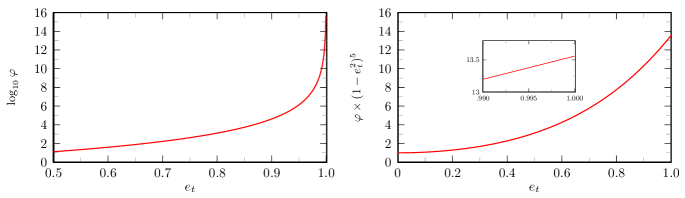
Figure 2: Enhancement function $\varphi(e_{t})$ associated with the 1.5PN tail. On the left the enhancement function is directly plotted, demonstrating the singular behavior as $e_{t}\rightarrow 1$. On the right, the eccentricity singular factor $(1-e_{t}^{2})^{-5}$ is removed to reveal convergence in the remaining expansion to a finite value of approximately $13.5586$ at $e_{t}=1$.

IV.2.2 Form of the 3PN Hereditary Terms

With a useful expansion of $\varphi(e_{t})$ in hand, we employ the same approach to the other hereditary terms. As a careful reading of Ref. Arun et al. (2008a) makes clear the most difficult contribution to calculate is (52), the correction of the 1.5PN tail showing up at 2.5PN order. Accordingly, we first consider the simpler 3PN case (53), which is the sum of the tail-of-the-tail and tail-squared terms Arun et al. (2008a). The part in (53) that requires further investigation is $\chi(e_{t})$. The infinite series for $\chi(e_{t})$ is shown in Arun et al. (2008a) to be

$$\chi(e_{t})=\frac{1}{4}\,\sum_{n=1}^{\infty}n^{2}\,\log\left(\frac{n}{2}\right)\,g(n,e_{t}).$$ (62)

The same technique as before is now applied to $\chi(e_{t})$ using the expansion (59) of $g(n,e_{t})$. The series will be singular at $e_{t}=1$, so factoring out the singular behavior is important. However, for reasons to be explained in Sec. IV.3, it proves essential in this case to remove the two strongest divergences. We find

$$\chi(e_{t})=-\frac{3}{2}F(e_{t})\log(1-e_{t}^{2}) +\frac{1}{(1-e_{t}^{2})^{13/2}}\,\Bigg{\{}\left[-\frac{3}{2}-\frac{77}{3}\log(2)+\frac{6561}{256}\log(3)\right]e_{t}^{2}$$ (63)

$$+\left[-22+\frac{34855}{64}\log(2)-\frac{295245}{1024}\log(3)\right]e_{t}^{4}$$

$$+\left[-\frac{6595}{128}-\frac{1167467}{192}\log(2)+\frac{24247269}{16384}\log(3)+\frac{244140625}{147456}\log(5)\right]e_{t}^{6}$$

$$+\left[-\frac{31747}{768}+\frac{122348557}{3072}\log(2)+\frac{486841509}{131072}\log(3)-\frac{23193359375}{1179648}\log(5)\right]e_{t}^{8}+\cdots\Bigg{\}}.$$

Empirically, we found the series for $\chi(e_{t})$ diverging like $\chi(e_{t})\sim-C_{\chi}(1-e_{t}^{2})^{-13/2}\log(1-e_{t}^{2})$ as $e_{t}\rightarrow 1$, where $C_{\chi}$ is a constant. The first term in (63) apparently encapsulates all of the logarithmic divergence and implies that $C_{\chi}=-(3/2)(52745/1024)\simeq-77.2632$. The reason for pulling out this particular function is based on a guess suggested by the asymptotic analysis in Sec. IV.3 and considerations on how logarithmically divergent terms in the combined instantaneous-plus-hereditary 3PN flux should cancel when a switch is made from orbital parameters $e_{t}$ and $y$ to parameters $e_{t}$ and $1/p$ (to be further discussed in a forthcoming paper). Having isolated the two divergent terms, the remaining series converges rapidly with $n$. The divergent behavior of the second term as $e_{t}\rightarrow 1$ is computed to be approximately $\simeq+73.6036(1-e_{t}^{2})^{-13/2}$. The appearance of $\chi(e_{t})$ is shown in Fig. 3, with and without its most singular factor removed.

IV.2.3 Form of the 2.5PN Hereditary Term

Armed with this success we went hunting for a comparable result for the 2.5PN enhancement factor $\psi$. Calculating $\psi$ is a much more involved process, as part of the tail at this order is a 1PN correction to the mass quadrupole. At 1PN order the orbital motion no longer closes and the corrections in the mass quadrupole moments require a biperiodic Fourier expansion. Arun et al. Arun et al. (2008b) describe a procedure for computing $\psi$, which they evaluated numerically. One of the successes we are able to report in this paper is having obtained a high-order power series expansion for $\psi$ in $e_{t}$. Even with Mathematica’s help, it is a consuming calculation, and we have reached only the 35th order ($e_{t}^{70}$). This achieves some of our purposes in seeking the expansion. We were also able to predict the comparable singular factor present as $e_{t}\rightarrow 1$ and demonstrate apparent convergence in the remaining series to a finite value at $e_{t}=1$. The route we followed in making the calculation of the 2.5PN tail is described in App. A. Here, we give the first few terms in the $\psi$ expansion

$$\psi(e_{t})=\frac{1}{\left(1-e_{t}^{2}\right)^{6}}\biggl{[}1 -\frac{72134}{8191}e_{t}^{2}-\frac{19817891}{524224}e_{t}^{4}-\frac{62900483}{4718016}e_{t}^{6}-\frac{184577393}{603906048}e_{t}^{8}+\frac{1052581}{419379200}e_{t}^{10}$$

$$-\frac{686351417}{1159499612160}e_{t}^{12}+\frac{106760742311}{852232214937600}e_{t}^{14}+\frac{7574993235161}{436342894048051200}e_{t}^{16}$$

$$-\frac{4345876114169}{2524555315563724800}e_{t}^{18}-\frac{61259745206138959}{56550039068627435520000}e_{t}^{20}+\cdots\biggr{]},$$ (64)

Like in the preceding plots, we show $\log_{10}|\psi|$ graphed on the left in Fig. 4. The singular behavior is evident. On the right side, the 2.5PN singular factor has been removed and the finite limit at $e_{t}=1$ is clear.

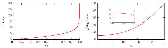
Figure 3: The 3PN enhancement function $\chi(e_{t})$. Its log is plotted on the left. On the right we remove the dominant singular factor $-(1-e_{t}^{2})^{-13/2}\log(1-e_{t}^{2})$. The turnover near $e_{t}=1$ reflects competition with the next-most-singular factor, $(1-e_{t}^{2})^{-13/2}$.

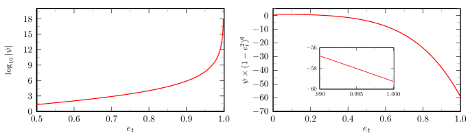
Figure 4: The enhancement factor $\psi(e_{t})$. On the right we remove the singular factor $(1-e_{t}^{2})^{-6}$ and see the remaining contribution smoothly approach a finite value at $e_{t}=1$.

IV.3 Applying asymptotic analysis to determine eccentricity singular factors

In the preceding section we assumed the existence of certain “correct” eccentricity singular factors in the behavior of the known hereditary terms, which once factored out allow the remaining power series to converge to constants at $e_{t}=1$. We show now that at least some of these singular factors, specifically the ones associated with $\varphi(e_{t})$ and $\chi(e_{t})$, can be derived via asymptotic analysis. In the process the same analysis confirms the singular factors in $f(e_{t})$ and $F(e_{t})$ already known from post-Newtonian work. As a bonus our asymptotic analysis can even be used to make remarkably sharp estimates of the limiting constant coefficients that multiply these singular factors.

What all four of these enhancement functions share is dependence on the square of the harmonics of the quadrupole moment given by the function $g(n,e_{t})$ found in (IV.2). To aid our analysis near $e_{t}=1$, we define $x\equiv 1-e_{t}^{2}$ and use $x$ to rewrite (IV.2) as

$$g(n,e_{t})=\frac{1}{6}n^{2}\frac{1+x+x^{2}+3n^{2}x^{3}}{(1-x)^{2}}J_{n}(ne_{t})^{2}+\frac{1}{2}n^{2}\frac{x(1+n^{2}x)}{1-x}J_{n}^{\prime}(ne_{t})^{2}-\frac{1}{2}n^{3}\frac{x(1+3x)}{(1-x)^{3/2}}J_{n}(ne_{t})J_{n}^{\prime}(ne_{t}).$$ (65)

An inspection of how (65) folds into (55), (57), (58), and (62) shows that infinite sums of the following forms are required to compute $\varphi(e_{t})$, $\chi(e_{t})$, $f(e_{t})$, and $F(e_{t})$

$$H_{0}^{\alpha,\beta}=\sum_{n=1}^{\infty}n^{\alpha}\log^{\beta}\left(\frac{n}{2}\right)J_{n}(ne_{t})^{2},\quad H_{1}^{\alpha,\beta}=\sum_{n=1}^{\infty}n^{\alpha}\log^{\beta}\left(\frac{n}{2}\right)J_{n}^{\prime}(ne_{t})^{2},\quad H_{2}^{\alpha,\beta}=\sum_{n=1}^{\infty}n^{\alpha}\log^{\beta}\left(\frac{n}{2}\right)J_{n}(ne_{t})J_{n}^{\prime}(ne_{t}).$$ (66)

In this compact shorthand, $\beta=1$ merely indicates sums that contain logs needed to calculate $\chi(e_{t})$ while $\beta=0$ (absence of a log) covers the other cases. Careful inspection of (65) reveals there are 18 different sums needed to calculate the four enhancement functions in question, and $\alpha$ ranges over (some) values between $2$ and $6$.

As $x\rightarrow 0$ ($e_{t}\rightarrow 1$) large $n$ terms have growing importance in the sums. In this limit the Bessel functions have uniform asymptotic expansions for large order $n$ of the form Abramowitz and Stegun (1972); DLMF ; Olver et al. (2010a)

$$J_{n}(ne_{t})\sim \left(\frac{4\zeta}{x}\right)^{\frac{1}{4}}\left[n^{-1/3}{\rm Ai}(n^{2/3}\zeta)\sum_{k=0}^{\infty}\frac{A_{k}}{n^{2k}}+n^{-5/3}{\rm Ai^{\prime}}(n^{2/3}\zeta)\sum_{k=0}^{\infty}\frac{B_{k}}{n^{2k}}\right],$$ (67)

$$J_{n}^{\prime}(ne_{t})\sim -\frac{2}{\sqrt{1-x}}\left(\frac{x}{4\zeta}\right)^{\frac{1}{4}}\left[n^{-4/3}{\rm Ai}(n^{2/3}\zeta)\sum_{k=0}^{\infty}\frac{C_{k}}{n^{2k}}+n^{-2/3}{\rm Ai^{\prime}}(n^{2/3}\zeta)\sum_{k=0}^{\infty}\frac{D_{k}}{n^{2k}}\right],$$ (68)

where $\zeta$ depends on eccentricity and is found from

$$\frac{2}{3}\zeta^{3/2}=\log\left(\frac{1+\sqrt{x}}{\sqrt{1-x}}\right)-\sqrt{x}\equiv\rho(x)\simeq\frac{1}{3}x^{3/2}+\frac{1}{5}x^{5/2}+\frac{1}{7}x^{7/2}+\cdots,$$ (69)

and where the expansion of $\rho(x)$ is the Puiseux series. Defining $\xi\equiv n\rho(x)$, we need in turn the asymptotic expansions of the Airy functions Abramowitz and Stegun (1972); DLMF ; Olver et al. (2010a)

$${\rm Ai}(n^{2/3}\zeta)\sim \,\frac{e^{-\xi}}{2^{5/6}3^{1/6}\sqrt{\pi}\xi^{1/6}}\left(1-\frac{5}{72\xi}+\frac{385}{10368\xi^{2}}-\frac{85085}{2239488\xi^{3}}+\frac{37182145}{644972544\xi^{4}}-\frac{5391411025}{46438023168\xi^{5}}+\cdots\right),$$ (70)

$${\rm Ai^{\prime}}(n^{2/3}\zeta)\sim \,-\frac{3^{1/6}\xi^{1/6}e^{-\xi}}{2^{7/6}\sqrt{\pi}}\left(1+\frac{7}{72\xi}-\frac{455}{10368\xi^{2}}+\frac{95095}{2239488\xi^{3}}-\frac{40415375}{644972544\xi^{4}}+\frac{5763232475}{46438023168\xi^{5}}+\cdots\right).$$ (71)

In some of the following estimates all six leading terms in the Airy function expansions are important, while a careful analysis reveals that we never need to retain any terms in the Bessel function expansions beyond $A_{0}=1$ and $D_{0}=1$.

These asymptotic expansions can now be used to analyze the behavior of the sums in (66) (from whence follow the enhancement functions) in the limit as $e_{t}\rightarrow 1$. Take as an example $H_{2}^{3,0}$. We replace the Bessel functions with their asymptotic expansions and thus obtain an approximation for the sum

$$H_{2}^{3,0}=\sum_{n=1}^{\infty}n^{3}J_{n}(ne_{t})J_{n}^{\prime}(ne_{t})\simeq\frac{1}{2\pi\sqrt{1-x}}\sum_{n=1}^{\infty}n^{2}e^{-2\xi}\left(1+\frac{1}{36\xi}-\frac{35}{2592\xi^{2}}+\cdots\right),$$ (72)

where recall that $\xi$ is the product of $n$ with $\rho(x)$. The original sum has in fact a closed form that can be found in the appendix of Peters and Mathews (1963)

$$\sum_{n=1}^{\infty}n^{3}J_{n}(ne_{t})J_{n}^{\prime}(ne_{t})=\frac{e_{t}}{4(1-e_{t}^{2})^{9/2}}\left(1+3~{}e_{t}^{2}+\frac{3}{8}~{}e_{t}^{4}\right)\sim\frac{35}{32}\,\frac{1}{(1-e_{t}^{2})^{9/2}}\simeq\frac{1.094}{(1-e_{t}^{2})^{9/2}},$$ (73)

where in the latter part of this line we give the behavior near $e_{t}=1$. With this as a target, we take the approximate sum in (72) and make a further approximation by replacing the sum over $n$ with an integral over $\xi$ from $0$ to $\infty$ while letting $\Delta n=1\rightarrow d\xi/\rho(x)$ and retaining only terms in the expansion that yield non-divergent integrals. We find

$$\frac{1}{2\pi\sqrt{1-x}}\frac{1}{\rho(x)^{3}}\int_{0}^{\infty}d\xi\,e^{-2\xi}\,\left(\xi^{2}+\frac{1}{36}\xi-\frac{35}{2592}\right)=\frac{1297}{10368\,\pi}\frac{1}{\rho(x)^{3}\sqrt{1-x}}\sim\frac{1297}{384\,\pi}\frac{1}{(1-e_{t}^{2})^{9/2}}\simeq\frac{1.0751}{(1-e_{t}^{2})^{9/2}},$$ (74)

with the final result coming from further expanding in powers of $x$. Our asymptotic calculation, and approximate replacement of sum with integral, not only provides the known singular dependence but also an estimate of the coefficient on the singular term that is better than we perhaps had any reason to expect.

All of the remaining 17 sums in (66) can be approximated in the same way. As an aside it is worth noting that for those sums in (66) without log terms (i.e., $\beta=0$) the replacement of the Bessel functions with their asymptotic expansions leads to infinite sums that can be identified as the known polylogarithm functions DLMF ; Olver et al. (2010a)

$${\rm Li}_{-k}\left(e^{-2\rho(x)}\right)=\sum_{n=1}^{\infty}n^{k}e^{-2n\rho(x)}.$$ (75)

However, expanding the polylogarithms as $x\rightarrow 0$ provides results for the leading singular dependence that are no different from those of the integral approximation. Since the $\beta=1$ cases are not represented by polylogarithms, we simply uniformly use the integral approximation.

We can apply these estimates to the four enhancement functions. First, the Peters-Mathews function $f(e_{t})$ in (55) has known leading singular dependence of

$$f(e_{t})\simeq\left(1+\frac{73}{24}+\frac{37}{96}\right)\frac{1}{(1-e_{t}^{2})^{7/2}}=\frac{425}{96}\frac{1}{(1-e_{t}^{2})^{7/2}}\simeq\frac{4.4271}{(1-e_{t}^{2})^{7/2}},\qquad{\rm as}\qquad e_{t}\rightarrow 1.$$ (76)

If we instead make an asymptotic analysis of the sum in (55) we find

$$f(e_{t})\sim\frac{191755}{13824\,\pi}\frac{1}{(1-e_{t}^{2})^{7/2}}\simeq\frac{4.4153}{(1-e_{t}^{2})^{7/2}},$$ (77)

which extracts the correct eccentricity singular function and yields a surprisingly sharp estimate of the coefficient. We next turn to the function $F(e_{t})$ in (57). In this case the function tends to $F(e_{t})\simeq(52745/1024)(1-e_{t}^{2})^{-13/2}\simeq 51.509(1-e_{t}^{2})^{-13/2}$ as $e_{t}\rightarrow 1$. Using instead the asymptotic technique we get an estimate

$$F(e_{t})\sim\frac{5148642773}{31850496\,\pi}\frac{1}{(1-e_{t}^{2})^{13/2}}\simeq\frac{51.455}{(1-e_{t}^{2})^{13/2}}.$$ (78)

Once again the correct singular function emerges and a surprisingly accurate estimate of the coefficient is obtained.

These two cases are heartening checks on the asymptotic analysis but of course both functions already have known closed forms. What is more interesting is to apply the approach to $\varphi(e_{t})$ and $\chi(e_{t})$, which are not known analytically. For the sum in (58) for $\varphi(e_{t})$ we obtain the following asymptotic estimate

$$\varphi(e_{t})\sim\frac{56622073}{1327104\,\pi}\frac{1}{(1-e_{t}^{2})^{5}}-\frac{371833517}{6635520\,\pi}\frac{1}{(1-e_{t}^{2})^{4}}+\cdots\simeq\frac{13.581}{(1-e_{t}^{2})^{5}}-\frac{17.837}{(1-e_{t}^{2})^{4}}+\cdots,$$ (79)

where in this case we retained the first two terms in the expansion about $e_{t}=1$. The leading singular factor is exactly the one we identified in IV.2.1 and its coefficient is remarkably close to the 13.5586 value found by numerically evaluating the high-order expansion in (61). The second term was retained merely to illustrate that the expansion is a regular power series in $x$ starting with $x^{-5}$ (in contrast to the next case).

We come finally to the enhancement function, $\chi(e_{t})$, whose definition (62) involves logarithms. Using the same asymptotic expansions and integral approximation for the sum, and retaining the first two divergent terms, we find

$$\chi(e_{t})\sim-\frac{5148642773}{21233664\,\pi}\frac{\log(1-e_{t}^{2})}{(1-e_{t}^{2})^{13/2}}-\frac{5148642773}{21233664\,\pi}\left[-\frac{7882453164}{5148642773}+\frac{2}{3}\gamma_{E}+\frac{4}{3}\log(2)-\frac{2}{3}\log(3)\right]\frac{1}{(1-e_{t}^{2})^{13/2}}.$$ (80)

The form of (63) assumed in Sec. IV.2.2, whose usefulness was verified through direct high-order expansion, was suggested by the leading singular behavior emerging from this asymptotic analysis. We guessed that there would be two terms, one with eccentricity singular factor $\log(1-e_{t}^{2})(1-e_{t}^{2})^{-13/2}$ and one with $(1-e_{t}^{2})^{-13/2}$. In any calculation made close to $e_{t}=1$ these two leading terms compete with each other, with the logarithmic term only winning out slowly as $e_{t}\rightarrow 1$. Prior to identifying the two divergent series we initially had difficulty with slow convergence of an expansion for $\chi(e_{t})$ in which only the divergent term with the logarithm was factored out. To see the issue, it is useful to numerically evaluate our approximation (80)

$$\chi(e_{t})\sim-77.1823\frac{\log(1-e_{t}^{2})}{(1-e_{t}^{2})^{13/2}}\left[1-\frac{0.954378}{\log(1-e_{t}^{2})}\right]=-77.1823\frac{\log(1-e_{t}^{2})}{(1-e_{t}^{2})^{13/2}}+\frac{73.6612}{(1-e_{t}^{2})^{13/2}}.$$ (81)

From this it is clear that even at $e_{t}=0.99$ the second term makes a $+24.3$% correction to the first term, giving the misleading impression that the leading coefficient is near $-96$ not $-77$. The key additional insight was to guess the closed form for the leading singular term in (63). As mentioned, the reason for expecting this exact relationship comes from balancing and cancelling logarithmic terms in both instantaneous and hereditary 3PN terms when the expansion is converted from one in $e_{t}$ and $y$ to one in $e_{t}$ and $1/p$. The coefficient on the leading (logarithmic) divergent term in $\chi(e_{t})$ is exactly $-(3/2)(52745/1024)\simeq-77.2632$. [This number is -3/2 times the limit of the polynomial in $F(e_{t})$.] It compares well with the first number in (81). Additionally, recalling the discussion made following (63), the actual coefficient found on the $(1-e_{t}^{2})^{-13/2}$ term is $+73.6036$, which compares well with the second number in (81). The asymptotic analysis has thus again provided remarkably sharp estimates for an eccentricity singular factor.

IV.4 Using Darwin eccentricity $e$ to map $\mathcal{I}(e_{t})$ and $\mathcal{K}(e_{t})$ to $\tilde{\mathcal{I}}(e)$ and $\tilde{\mathcal{K}}(e)$

Our discussion thus far has given the PN energy flux in terms of the standard QK time eccentricity $e_{t}$ in modified harmonic gauge Arun et al. (2009). The motion is only known presently to 3PN relative order, which means that the QK representation can only be transformed between gauges up to and including $y^{3}$ corrections. At the same time, our BHP calculations accurately include all relativistic effects that are first order in the mass ratio. It is possible to relate the relativistic (Darwin) eccentricity $e$ to the QK $e_{t}$ (in, say, modified harmonic gauge) up through correction terms of order $y^{3}$,

$$\frac{e_{t}^{2}}{e^{2}}= 1-6y-\frac{\left(15-19\sqrt{1-e^{2}}\right)+\left(15\sqrt{1-e^{2}}-15\right)e^{2}}{(1-e^{2})^{3/2}}y^{2}$$

$$\quad+\frac{1}{(1-e^{2})^{5/2}}\biggl{[}\left(30-38\sqrt{1-e^{2}}\right)+\left(59\sqrt{1-e^{2}}-75\right)e^{2}+\left(45-18\sqrt{1-e^{2}}\right)e^{4}\biggr{]}y^{3}.$$ (82)

See Arun et al. (2009) for the low-eccentricity limit of this more general expression. We do not presently know how to calculate $e_{t}$ beyond this order. Using this expression we can at least transform expected fluxes to their form in terms of $e$ and check current PN results through 3PN order. However, to go from 3PN to 7PN, as we do in this paper, our results must be given in terms of $e$.

The instantaneous ($\mathcal{I}$) and hereditary ($\mathcal{K}$) flux terms may be rewritten in terms of the relativistic eccentricity $e$ straightforwardly by substituting $e$ for $e_{t}$ using (IV.4) in the full 3PN flux (45) and re-expanding the result in powers of $y$. All flux coefficients that are lowest order in $y$ are unaffected by this transformation. Instead, only higher order corrections are modified. We find

$$\tilde{\mathcal{I}}_{0}(e) =\mathcal{I}_{0}(e_{t}),\qquad\tilde{\mathcal{K}}_{3/2}(e)=\mathcal{K}_{3/2}(e_{t}),\qquad\tilde{\mathcal{K}}_{3}(e)=\mathcal{K}_{3}(e_{t}),$$ (83)

$$\tilde{\mathcal{I}}_{1}(e) =\frac{1}{(1-e^{2})^{9/2}}\left(-\frac{1247}{336}-\frac{15901}{672}e^{2}-\frac{9253}{384}e^{4}-\frac{4037}{1792}e^{6}\right),$$ (84)

$$\tilde{\mathcal{I}}_{2}(e) =\frac{1}{(1-e^{2})^{11/2}}{\left(-\frac{203471}{9072}-\frac{1430873}{18144}e^{2}+\frac{2161337}{24192}e^{4}+\frac{231899}{2304}e^{6}+\frac{499451}{64512}e^{8}\right)}$$ (85)

$$\hskip 172.22168pt+\frac{1}{(1-e^{2})^{5}}\left(\frac{35}{2}+\frac{1715}{48}e^{2}-\frac{2975}{64}e^{4}-\frac{1295}{192}e^{6}\right),$$

$$\tilde{\mathcal{I}}_{3}(e) =\frac{1}{(1-e^{2})^{13/2}}\left(\frac{2193295679}{9979200}+\frac{55022404229}{19958400}e^{2}+\frac{68454474929}{13305600}e^{4}\right.$$ (86)

. $$\hskip 129.16626pt+\frac{40029894853}{26611200}e^{6}-\frac{32487334699}{141926400}e^{8}-\frac{233745653}{11354112}e^{10}\biggr{)}$$

$$\qquad+\frac{1}{(1-e^{2})^{6}}\left(-\frac{14047483}{151200}-\frac{75546769}{100800}e^{2}-\frac{210234049}{403200}e^{4}+\frac{1128608203}{2419200}e^{6}+\frac{617515}{10752}e^{8}\right)$$

$$\qquad+\frac{1712}{105}\log\left[\frac{y}{y_{0}}\frac{1+\sqrt{1-e^{2}}}{2(1-e^{2})}\right]F(e),$$

$$\tilde{\mathcal{K}}_{5/2}(e) =\frac{-\pi}{(1-e^{2})^{6}}\biggl{(}\frac{8191}{672}+\frac{62003}{336}e^{2}+\frac{20327389}{43008}e^{4}+\frac{87458089}{387072}e^{6}+\frac{67638841}{7077888}e^{8}+\frac{332887}{25804800}e^{10}$$

$$\hskip 86.11084pt-\frac{482542621}{475634073600}e^{12}+\frac{43302428147}{69918208819200}e^{14}-\frac{2970543742759}{35798122915430400}e^{16}$$

$$\hskip 86.11084pt+\frac{3024851376397}{207117711153561600}e^{18}+\frac{24605201296594481}{4639436729839779840000}e^{20}+\cdots\biggr{)},$$ (87)

where $F$ is given by (50) with $e_{t}\rightarrow e$. The full 3PN flux is written exactly as Eqn. (45) with $\mathcal{I}\to\tilde{\mathcal{I}}$ and $\mathcal{K}\to\tilde{\mathcal{K}}$.

V Confirming eccentric-orbit fluxes through 3PN relative order

Sections II and III briefly described a formalism for an efficient, arbitrary-precision MST code for use with eccentric orbits. Section IV detailed new high-order expansions in $e^{2}$ that we have developed for the hereditary PN terms. The next goal of this paper is to check all known PN coefficients for the energy flux (at lowest order in the mass ratio) for eccentric orbits. The MST code is written in Mathematica to allow use of its arbitrary precision functions. Like previous circular orbit calculations Shah et al. (2014); Shah (2014a), we employ very high accuracy calculations (here up to 200 decimal places of accuracy) on orbits with very wide separations ($p\simeq 10^{15}-10^{35}$). Why such wide separations? At $p=10^{20}$, successive terms in a PN expansion separate by 20 decimal places from each other (10 decimal places for half-PN order jumps). It is like doing QED calculations and being able to dial down the fine structure constant from $\alpha\simeq 1/137$ to $10^{-20}$. This in turn mandates the use of exceedingly high-accuracy calculations; it is only by calculating with 200 decimal places that we can observe $\sim 10$ PN orders in our numerical results with some accuracy.

V.1 Generating numerical results with the MST code

In Secs. II and III we covered the theoretical framework our code uses. We now provide an algorithmic roadmap for the code. (While the primary focus of this paper is in computing fluxes, the code is also capable of calculating local quantities to the same high accuracy.)

• Solve orbit equations for given $p$ and $e$. Given a set of orbital parameters, we find $t_{p}(\chi)$, $\varphi_{p}(\chi)$, and $r_{p}(\chi)$ to high accuracy at locations equally spaced in $\chi$. We do so by employing the SSI method outlined in Sec. II B of Ref. Hopper et al. (2015). From these functions we also obtain the orbital frequencies $\Omega_{r}$ and $\Omega_{\varphi}$. All quantities are computed with some pre-determined overall accuracy goal; in this paper it was a goal of 200 decimal places of accuracy in the energy flux.

• Obtain homogeneous solutions to the FD RWZ master equation for given $lmn$ mode. We find the homogeneous solutions using the MST formalism outlined in Sec. II.2. The details of the calculation are given here.

  1. Solve for $\nu$. For each $lmn$, the $\omega$-dependent renormalized angular momentum $\nu$ is determined (App. B).

  2. Determine at what $n$ to truncate infinite MST sums involving $a_{n}$. The solutions $R_{lm\omega}^{\text{up/in}}$ are infinite sums (7) and (11). Starting with $a_{0}=1$, we determine $a_{n}$ for $n<0$ and $n>0$ using Eqn. (B). Terms are added on either side of $n=0$ until the homogeneous Teukolsky equation is satisfied to within some error criterion at a single point on the orbit. In the post-Newtonian regime the behavior of the size of these terms is well understood Mano et al. (1996a, b); Kavanagh et al. (2015). Our algorithm tests empirically for stopping. Note that in addition to forming $R_{lm\omega}^{\text{up/in}}$, residual testing requires computing its first and second derivatives. Having tested for validity of the stopping criterion at one point, we spot check at other locations around the orbit. Once the number of terms is established we are able to compute the Teukolsky function and its first derivative at any point along the orbit. (The index $n$ here is not to be confused with the harmonic index on such functions as $\hat{X}_{lmn}$.)

  3. Evaluate Teukolsky function between $r_{\rm min}$ and $r_{\rm max}$. Using the truncation of the infinite MST series, we evaluate $R_{lm\omega}^{\text{up/in}}$ and their first derivative [higher derivatives are found using the homogeneous differential equation (3)] at the $r$ locations corresponding to the even-$\chi$ spacing found in Step 1. The high precision evaluation of hypergeometric functions in this step represents the computational bottleneck in the code.

  4. Transform Teukolsky function to RWZ master functions. For $l+m$ odd we use Eqn. (15) to obtain $\hat{X}_{lmn}^{\pm}$. When $l+m$ is even we continue and use Eqn. (16).

  5. Scale master functions. In solving for the fluxes, it is convenient to work with homogeneous solutions that are unit-normalized at the horizon and at infinity. We divide the RWZ solutions by the asymptotic amplitudes that arise from choosing $a_{0}=1$ when forming the MST solutions to the Teukolsky equation. These asymptotic forms are given in Eqns. (17)-(LABEL:eqn:RWasymp3).

• Form $lmn$ flux contribution. Form $C_{lmn}^{+}$ using the exponentially-convergent SSI sum (43). Note that this exponential convergence relies on the fact that we evaluated the homogeneous solutions at evenly-spaced locations in $\chi$. The coefficient $C_{lmn}^{+}$ feeds into a single positive-definite term in the sum (44).

• Sum over $lmn$ modes. In reconstructing the total flux there are three sums:

  1. Sum over $n$. For each spherical harmonic $lm$, there is formally an infinite Fourier series sum from $n=-\infty$ to $\infty$. In practice the SSI method shows that $n$ is effectively bounded in some range $-N_{1}\leq n\leq N_{2}$. This range is determined by the fineness of the evenly-spaced sampling of the orbit in $\chi$. For a given orbital sampling, we sum modes between $-N_{1}\leq n\leq N_{2}$, where $N_{1}$ and $N_{2}$ are the first Nyquist-like notches in frequency, beyond which aliasing effects set in Hopper et al. (2015).

  2. Sum over $m$. For each $l$ mode, we sum over $m$ from $-l\leq m\leq l$. In practice, symmetry allows us to sum from $0\leq m\leq l$, multiplying positive $m$ contributions by 2.

  3. Sum over $l$. The sum over $l$ is, again, formally infinite. However, each multipole order appears at a higher PN order, the spacing of which depends on $1/p$. The leading $l=2$ quadrupole flux appears at $\mathcal{O}(p^{-5})$. For an orbit with $p=10^{20}$, the $l=3$ flux appears at a level 20 orders of magnitude smaller. Only contributions through $l\leq 12$ are necessary with this orbit and an overall precision goal of 200 digits. This cutoff in $l$ varies with different $p$.

V.2 Numerically confirming eccentric-orbit PN results through 3PN order

We now turn to confirming past eccentric-orbit PN calculations. The MST code takes as input the orbital parameters $p$ and $e$. Then $1/p$ is a small parameter. Expanding $dt_{p}/d\chi$ in (III.1) we find from (25)

$$\Omega_{r}=\frac{1}{M}\left(\frac{1-e^{2}}{p}\right)^{3/2}\left\{1-3\frac{1-e^{2}}{p}-\frac{3}{2}\frac{\sqrt{1-e^{2}}[5-2\sqrt{1-e^{2}}+e^{2}(-5+6\sqrt{1-e^{2}})]}{p^{2}}+\cdots\right\}.$$ (88)

Expanding (27) in similar fashion gives

$$\Omega_{\varphi}=\frac{1}{M}\left(\frac{1-e^{2}}{p}\right)^{3/2}\left\{1+3\frac{e^{2}}{p}-\frac{3}{4}\frac{\left[10(-1+\sqrt{1-e^{2}})+e^{2}(20-3\sqrt{1-e^{2}})+2e^{4}(-5+6\sqrt{1-e^{2}})\right]}{\sqrt{1-e^{2}}p^{2}}+\cdots\right\}.$$ (89)

Then given the definition of $y$ we obtain an expansion of $y$ in terms of $p$

$$y=\frac{1-e^{2}}{p}+\frac{2e^{2}(1-e^{2})}{p^{2}}+\frac{1}{2}\sqrt{1-e^{2}}\frac{\left[10(1-\sqrt{1-e^{2}})+e^{2}(-3+10\sqrt{1-e^{2}})+10e^{4})\right]}{p^{3}}+\cdots.$$ (90)

So from our chosen parameters $e$ and $p$ we can obtain $y$ to arbitrary accuracy, and then other orbital parameters, such as $\Omega_{r}$ and $\Omega_{\varphi}$, can be computed as well to any desired accuracy.

Figure 5: Fourier-harmonic energy-flux spectra from an orbit with semi-latus rectum $p=10^{20}$ and eccentricity $e=0.1$. Each inverted-$V$ spectrum represents flux contributions of modes with various harmonic number $n$ but fixed $l$ and $m$. The tallest spectrum traces the harmonics of the $l=2$, $m=2$ quadrupole mode, the dominant contributor to the flux. Spectra of successively higher multipoles (octupole, hexadecapole, etc) each drop 20 orders of magnitude in strength as $l$ increases by one ($l\leq 12$ are shown). Every flux contribution is computed that is within 200 decimal places of the peak of the quadrupole spectrum. With $e=0.1$, there were 7,418 significant modes that had to be computed (and are shown above).

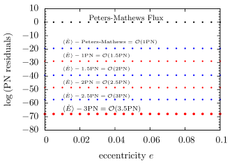
Figure 6: Residuals after subtracting from the numerical data successive PN contributions. Residuals are shown for a set of orbits with $p=10^{20}$ and a range of eccentricities from $e=0.005$ through $e=0.1$ in steps of $0.005$. Residuals are scaled relative to the Peters-Mathews flux (uppermost points at unit level). The next set of points (blue) shows residuals after subtracting the Peters-Mathews enhancement from BHP data. Residuals drop uniformly by 20 order of magnitude, consistent with 1PN corrections in the data. The next (red) points result from subtracting the 1PN term, giving residuals at the 1.5PN level. Successive subtraction of known PN terms is made, reaching final residuals at 70 orders of magnitude below the total flux and indicating the presence of 3.5PN contributions in the numerical fluxes.

To check past work Arun et al. (2008a, b, 2009); Blanchet (2014) on the PN expansion of the energy flux, we used a single orbital separation ($p=10^{20}$), with a set of eccentricities ($e=0.005$ through $e=0.1$). For each $e$, we compute the flux for each $lmn$-mode up to $l=12$ to as much as 200 decimal places of accuracy (the accuracy can be relaxed for higher $l$ as these modes contribute only weakly to the total energy flux). Fig. 6 depicts all 7,418 $lmn$-modes that contributed to the energy flux for just the $p=10^{20}$, $e=0.1$ orbit. Making this calculation and sum for all $e$, we then have an eccentricity dependent flux. Next, we compute the PN parts of the expected flux using Eqns. (83) through (IV.4). The predicted flux $\mathcal{F}_{\rm 3PN}$ is very close to the computed flux $\mathcal{F}_{\rm MST}$. We then subtract the quadrupole theoretical flux term

$$\mathcal{F}_{\rm N}=\frac{32}{5}\left(\frac{\mu}{M}\right)^{2}y^{5}\,\tilde{\mathcal{I}}_{0}(e)\equiv\mathcal{F}^{\rm circ}_{\rm N}\ \tilde{\mathcal{I}}_{0}(e),$$ (91)

from the flux computed with the MST code (and normalize with respect to the Newtonian term)

$$\frac{\mathcal{F}_{\rm MST}-\mathcal{F}_{\rm N}}{\mathcal{F}_{\rm N}}=\mathcal{O}(y)\simeq\frac{1}{\tilde{\mathcal{I}}_{0}(e)}\left[y\,\tilde{\mathcal{I}}_{1}(e)+y^{3/2}\,\tilde{\mathcal{K}}_{3/2}(e)+y^{2}\,\tilde{\mathcal{I}}_{2}(e)+y^{5/2}\,\tilde{\mathcal{K}}_{5/2}(e)+y^{3}\,\tilde{\mathcal{I}}_{3}(e)+y^{3}\,\tilde{\mathcal{K}}_{3}(e)\right],$$ (92)

and find a residual that is 20 orders of magnitude smaller than the quadrupole flux. The residual reflects the fact that our numerical (MST code) data contains the 1PN and higher corrections. We next subtract the 1PN term

$$\frac{\mathcal{F}_{\rm MST}-\mathcal{F}_{\rm N}}{\mathcal{F}_{\rm N}}-y\,\frac{\tilde{\mathcal{I}}_{1}(e)}{\tilde{\mathcal{I}}_{0}(e)}=\mathcal{O}(y^{3/2}),$$ (93)

and find residuals that are another 10 orders of magnitude lower. This reflects the expected 1.5PN tail correction. Using our high-order expansion for $\varphi(e)$, we subtract and reach 2PN residuals. Continuing in this way, once the 3PN term is subtracted, the residuals lie at a level 70 orders of magnitude below the quadrupole flux. We have reached the 3.5PN contributions, which are encoded in the MST result but whose form is (heretofore) unknown. Fig. 6 shows this process of successive subtraction. We conclude that the published PN coefficients Arun et al. (2008a); Blanchet (2014) for eccentric orbits in the lowest order in $\nu$ limit are all correct. Any error would have to be at the level of one part in $10^{10}$ (and only then in the 3PN terms) or it would show up in the residuals.

As a check we made this comparison also for other orbital radii and using the original expressions in terms of $e_{t}$ (which we computed from $e$ and $y$ to high precision). The 2008 results Arun et al. (2008a) continued to stand.

VI Determining new PN terms between orders 3.5PN and 7PN

Having confirmed theoretical results through 3PN, we next sought to determine analytic or numerical coefficients for as-yet unknown PN coefficients at 3.5PN and higher orders. We find new results to 7PN order.

VI.1 A model for the higher-order energy flux

The process begins with writing an expected form for the expansion. As discussed previously, beyond 3PN we presently do not know $e_{t}$, so all new results are parameterized in terms of the relativistic $e$ (and $y$). Based on experience with the expansion up to 3PN (and our expansions of the hereditary terms), we build in the expected eccentricity singular factors from the outset. In addition, with no guidance from analytic PN theory, we have no way of separating instantaneous from hereditary terms beyond 3PN order, and thus denote all higher-order PN enhancement factors with the notation $\mathcal{L}_{i}(e)$. Finally, known higher-order work Fujita (2012) in the circular-orbit limit allows us to anticipate the presence of various logarithmic terms and powers of logs. Accordingly, we take the flux to have the form

$$\left\langle\frac{dE}{dt}\right\rangle= \mathcal{F}_{\rm 3PN}+\mathcal{F}^{\rm circ}_{\rm N}\biggl{[}\mathcal{L}_{7/2}y^{7/2}+y^{4}\Bigl{(}\mathcal{L}_{4}+\log(y)\mathcal{L}_{4L}\Bigr{)}+y^{9/2}\Bigl{(}\mathcal{L}_{9/2}+\log(y)\mathcal{L}_{9/2L}\Bigr{)}+y^{5}\Bigl{(}\mathcal{L}_{5}+\log(y)\mathcal{L}_{5L}\Bigr{)}$$

$$\quad+y^{11/2}\Bigl{(}\mathcal{L}_{11/2}+\log(y)\mathcal{L}_{11/2L}\Bigr{)}+y^{6}\Bigl{(}\mathcal{L}_{6}+\log(y)\mathcal{L}_{6L}+\log^{2}(y)\mathcal{L}_{6L^{2}}\Bigr{)}+y^{13/2}\Bigl{(}\mathcal{L}_{13/2}+\log(y)\mathcal{L}_{13/2L}\Bigr{)}$$

$$\quad+y^{7}\Bigl{(}\mathcal{L}_{7}+\log(y)\mathcal{L}_{7L}+\log^{2}(y)\mathcal{L}_{7L^{2}}\Bigr{)}+y^{15/2}\Bigl{(}\mathcal{L}_{15/2}+\log(y)\mathcal{L}_{15/2L}+\log^{2}(y)\mathcal{L}_{15/2L^{2}}\Bigr{)}$$

$$\quad+y^{8}\Bigl{(}\mathcal{L}_{8}+\log(y)\mathcal{L}_{8L}+\log^{2}(y)\mathcal{L}_{8L^{2}}\Bigr{)}+y^{17/2}\Bigl{(}\mathcal{L}_{17/2}+\log(y)\mathcal{L}_{17/2L}+\log^{2}(y)\mathcal{L}_{17/2L^{2}}\Bigr{)}$$

$$\quad+y^{9}\Bigl{(}\mathcal{L}_{9}+\log(y)\mathcal{L}_{9L}+\log^{2}(y)\mathcal{L}_{9L^{2}}+\log^{3}(y)\mathcal{L}_{9L^{3}}\Bigr{)}$$

$$\quad+y^{19/2}\Bigl{(}\mathcal{L}_{19/2}+\log(y)\mathcal{L}_{19/2L}+\log^{2}(y)\mathcal{L}_{19/2L^{2}}+\log^{3}(y)\mathcal{L}_{19/2L^{3}}\Bigr{)}$$

$$\quad+y^{10}\Bigl{(}\mathcal{L}_{10}+\log(y)\mathcal{L}_{10L}+\log^{2}(y)\mathcal{L}_{10L^{2}}+\log^{3}(y)\mathcal{L}_{10L^{3}}\Bigr{)}\biggr{]}.$$ (94)

It proves useful to fit MST code data all the way through 10PN order even though we quote new results only up to 7PN.

VI.2 Roadmap for fitting the higher-order PN expansion

The steps in making a sequence of fits to determine the higher-order PN expansion are as follows:

• Compute data for orbits with various $e$ and $y$. We compute fluxes for 1,683 unique orbits, with 33 eccentricities for each of 51 different orbital separations ($p$ or $y$ values). The models include circular orbits and eccentricities ranging from $e=10^{-5}$ to $e=0.1$. The $p$ range is from $10^{10}$ through $10^{35}$ in half-logarithmic steps, i.e., $10^{10},10^{10.5},\dots$. The values of $y$ are derived from $p$ and $e$.

• Use the expected form of the expansion in $y$. As mentioned earlier, known results for circular fluxes on Schwarzschild backgrounds allow us to surmise the expected terms in the $y$-expansion, shown in Eqn. (VI.1). The expansion through 10PN order contains as a function of $y$ 44 parameters, which can be determined by our dataset with 51 $y$ values (at each eccentricity).

• Eliminate known fit parameters. The coefficients at 0PN, 1PN, 1.5PN, 2PN, and 3PN relative orders involve known enhancement functions of the eccentricity $e$ (given in the previous section) and these terms may be subtracted from the data and excluded from the fit model. It is important to note that we do not include the 2.5PN term in this subtraction. Though we have a procedure for expanding the $\mathcal{K}_{5/2}$ term to high order in $e^{2}$, it has proven computationally difficult so far to expand beyond $e^{70}$. This order was sufficient for use in Sec. V in confirming prior results to 3PN but is not accurate enough to reach 10PN (at the large radii we use). We instead include a parameterization of $\mathcal{K}_{5/2}$ in the fitting model.

• Fit for the coefficients on powers of $y$ and $\log(y)$. We use Mathematica’s NonlinearModelFit function to obtain numerical values for the coefficients $\mathcal{L}_{7/2}$, $\mathcal{L}_{4}$, $\dots$ shown in Eqn. (VI.1). We perform this fit separately for each of the 33 values of $e$ in the dataset.

• Organize the numerically determined functions of $e$ for each separate coefficient $\mathcal{L}_{i}(e)$ in the expansion over $y$ and $\log(y)$. Having fit to an expansion of the form (VI.1) and eliminated known terms there remain 38 functions of $e$, each of which is a discrete function of 33 different eccentricities.

• Assemble an expected form for the expansion in $e$ of each $\mathcal{L}_{i}(e)$. Based on the pattern in Sec. IV, each full (or half) PN order $=N$ will have a leading eccentricity singular factor of the form $(1-e^{2})^{-7/2-N}$. The remaining power series will be an expansion in powers of $e^{2}$.

• Fit each model for $\mathcal{L}_{i}(e)$ using data ranging over eccentricity. The function NonlinearModelFit is again used to find the unknown coefficients in the eccentricity function expansions. With data on 33 eccentricities, the coefficient models are limited to at most 33 terms. However, it is possible to do hierarchical fitting. As lower order coefficients are firmly determined in analytic form (see next step), they can be eliminated in the fitting model to allow new, higher-order ones to be included.

• Attempt to determine analytic form of $e^{2}$ coefficients. It is possible in some cases to determine the exact analytic form (rational or irrational) of coefficients of $e^{2}$ determined only in decimal value form in the previous step. We use Mathematica’s function FindIntegerNullVector (hereafter FINV), which is an implementation of the PSLQ integer-relation algorithm.

• Assess the validity of the analytic coefficients. A rational or irrational number, or combination thereof, predicted by FINV to represent a given decimal number has a certain probability of being a coincidence (note: the output of FINV will still be a very accurate representation of the input decimal number). If FINV outputs, say, a single rational number with $N_{N}$ digits in its numerator and $N_{D}$ digits in its denominator, and this rational agrees with the input decimal number it purports to represent to $N$ digits, then the likelihood that this is a coincidence is of order $\mathcal{P}\simeq 10^{N_{N}+N_{D}-N}$ Shah et al. (2014). With the analytic coefficients we give in what follows, in no case is the probability of coincidence larger than $10^{-6}$, and in many cases the probability is as low as $10^{-90}-10^{-50}$. Other consistency checks are made as well. It is important that the analytic output of PSLQ not change when the number of significant digits in the input is varied (within some range). Furthermore, as we expect rational numbers in a perturbation expansion to be sums of simpler rationals, a useful criterion for validity of an experimentally determined rational is that it have no large prime factors in its denominator Johnson-McDaniel et al. (2015).

VI.3 The energy flux through 7PN order

We now give, in mixed analytic and numeric form, the PN expansion (at lowest order in $\nu$) for the energy flux through 7PN order. Analytic coefficients are given directly, while well-determined coefficients that are known only in numerical form are listed in the formulae as numbered parameters like $b_{26}$. The numerical values of these coefficients are tabulated in App. C. We find for the 3.5PN and 4PN (non-log) terms

$$\mathcal{L}_{7/2} =-\frac{\pi}{(1-e^{2})^{7}}\biggl{(}\frac{16285}{504}+\frac{21500207}{48384}e^{2}+\frac{3345329}{48384}e^{4}-\frac{111594754909}{41803776}e^{6}-\frac{82936785623}{55738368}e^{8}-\frac{11764982139179}{107017666560}e^{10}$$

$$\ -\frac{216868426237103}{9631589990400}e^{12}-\frac{30182578123501193}{2517055517491200}e^{14}-\frac{351410391437739607}{48327465935831040}e^{16}-\frac{1006563319333377521717}{208774652842790092800}e^{18}$$

$$\ -\frac{138433556497603036591}{40776299383357440000}e^{20}-\frac{16836217054749609972406421}{6736462131727360327680000}e^{22}-\frac{2077866815397007172515220959}{1091306865339832373084160000}e^{24}$$

$$\ +b_{26}e^{26}+b_{28}e^{28}+b_{30}e^{30}+b_{32}e^{32}+b_{34}e^{34}+b_{36}e^{36}+b_{38}e^{38}+b_{40}e^{40}+b_{42}e^{42}+b_{44}e^{44}+b_{46}e^{46}+b_{48}e^{48}$$

$$\ +b_{50}e^{50}+b_{52}e^{52}+b_{54}e^{54}+\cdots\biggr{)},$$ (95)

$$\mathcal{L}_{4} =\frac{1}{(1-e^{2})^{15/2}}\biggl{[}-\frac{323105549467}{3178375200}+\frac{232597}{4410}\gamma_{\text{E}}-\frac{1369}{126}\pi^{2}+\frac{39931}{294}\log(2)-\frac{47385}{1568}\log(3)$$

$$\ +\biggl{(}-\frac{128412398137}{23543520}+\frac{4923511}{2940}\gamma_{\text{E}}-\frac{104549}{252}\pi^{2}-\frac{343177}{252}\log(2)+\frac{55105839}{15680}\log(3)\biggr{)}e^{2}$$

$$\ +\biggl{(}-\frac{981480754818517}{25427001600}+\frac{142278179}{17640}\gamma_{\text{E}}-\frac{1113487}{504}\pi^{2}+\frac{762077713}{5880}\log(2)-\frac{2595297591}{71680}\log(3)$$

$$\hskip 107.63855pt-\frac{15869140625}{903168}\log(5)\biggr{)}e^{4}$$

$$\ +\biggl{(}-\frac{874590390287699}{12713500800}+\frac{318425291}{35280}\gamma_{\text{E}}-\frac{881501}{336}\pi^{2}-\frac{90762985321}{63504}\log(2)+\frac{31649037093}{1003520}\log(3)$$

$$\hskip 107.63855pt+\frac{10089048828125}{16257024}\log(5)\biggr{)}e^{6}$$

$$\ +d_{8}e^{8}+d_{10}e^{10}+d_{12}e^{12}+d_{14}e^{14}+d_{16}e^{16}+d_{18}e^{18}+d_{20}e^{20}+d_{22}e^{22}+d_{24}e^{24}+d_{26}e^{26}$$

$$\ +d_{28}e^{28}+d_{30}e^{30}+d_{32}e^{32}+d_{34}e^{34}+d_{36}e^{36}+d_{38}e^{38}+d_{40}e^{40}+\cdots\biggr{]}.$$ (96)

In both of these expressions the circular orbit limits ($e^{0}$) were known Fujita (2012). These results have been presented earlier Forseth (2014, 2015); Evans (2015) and are available online. The coefficients through $e^{6}$ for 3.5PN and 4PN are also discussed in Sago and Fujita (2015), which we found to be in agreement with our results. We next consider the 4PN log contribution, which we find to have an exact, closed-form expression

$$\mathcal{L}_{4L} =\frac{1}{(1-e^{2})^{15/2}}\biggl{(}\frac{232597}{8820}+\frac{4923511}{5880}e^{2}+\frac{142278179}{35280}e^{4}+\frac{318425291}{70560}e^{6}+\frac{1256401651}{1128960}e^{8}+\frac{7220691}{250880}e^{10}\biggr{)}.$$ (97)

In the 4.5PN non-log term we were only able to find analytic coefficients for the circular limit (known previously) and the $e^{2}$ term. We find many higher-order terms numerically (App. C)

$$\mathcal{L}_{9/2} =\frac{\pi}{(1-e^{2})^{8}}\biggl{[}\frac{265978667519}{745113600}-\frac{6848}{105}\gamma_{\text{E}}-\frac{13696}{105}\log(2)+\biggl{(}\frac{5031659060513}{447068160}-\frac{418477}{252}\gamma_{\text{E}}-\frac{1024097}{1260}\log(2)$$

$$\ -\frac{702027}{280}\log(3)\biggr{)}e^{2}+h_{4}e^{4}+h_{6}e^{6}+h_{8}e^{8}+h_{10}e^{10}+h_{12}e^{12}+h_{14}e^{14}+h_{16}e^{16}+h_{18}e^{18}+h_{20}e^{20}+h_{22}e^{22}$$

$$\ +h_{24}e^{24}+h_{26}e^{26}+h_{28}e^{28}+h_{30}e^{30}+h_{32}e^{32}+h_{34}e^{34}+h_{36}e^{36}\biggr{]}.$$ (98)

In the 4.5PN log term we are able to find the first 10 coefficients in analytic form and 6 more in accurate numerical form (App. C)

$$\mathcal{L}_{9/2L} =-\frac{\pi}{(1-e^{2})^{8}}\biggl{(}\frac{3424}{105}+\frac{418477}{504}e^{2}+\frac{32490229}{10080}e^{4}+\frac{283848209}{96768}e^{6}+\frac{1378010735}{2322432}e^{8}+\frac{59600244089}{4644864000}e^{10}$$

$$\ -\frac{482765917}{7962624000}e^{12}+\frac{532101153539}{29132587008000}e^{14}-\frac{576726373021}{199766310912000}e^{16}+\frac{98932878601597}{3624559945187328000}e^{18}+g_{20}e^{20}$$

$$\ +g_{22}e^{22}+g_{24}e^{24}+g_{26}e^{26}+g_{28}e^{28}+g_{30}e^{30}+\cdots\biggr{)}.$$ (99)

For the 5PN non-log term, we are only able to confirm the circular-orbit limit analytically. Many other terms were found with accurate numerical values (App. C)

$$\mathcal{L}_{5} =\frac{1}{(1-e^{2})^{17/2}}\biggl{[}-\frac{2500861660823683}{2831932303200}-\frac{424223}{6804}\pi^{2}+\frac{916628467}{7858620}\gamma_{\text{E}}-\frac{83217611}{1122660}\log(2)+\frac{47385}{196}\log(3)$$

$$\ +k_{2}e^{2}+k_{4}e^{4}+k_{6}e^{6}+k_{8}e^{8}+k_{10}e^{10}+k_{12}e^{12}+k_{14}e^{14}+k_{16}e^{16}+k_{18}e^{18}+k_{20}e^{20}+k_{22}e^{22}+k_{24}e^{24}$$

$$\ +k_{26}e^{26}+\cdots\biggr{]}.$$ (100)

In the 5PN log term we found the first 13 terms in analytic form, and several more numerically (App. C)

$$\mathcal{L}_{5L} =\frac{1}{(1-e^{2})^{17/2}}\biggl{(}\frac{916628467}{15717240}+\frac{11627266729}{31434480}e^{2}-\frac{84010607399}{10478160}e^{4}-\frac{67781855563}{1632960}e^{6}-\frac{87324451928671}{2011806720}e^{8}$$

$$\ -\frac{301503186907}{29804544}e^{10}-\frac{752883727}{1290240}e^{12}-\frac{22176713}{129024}e^{14}-\frac{198577769}{2064384}e^{16}-\frac{250595605}{4128768}e^{18}$$

$$\ -\frac{195002899}{4718592}e^{20}-\frac{280151573}{9437184}e^{22}-\frac{1675599991}{75497472}e^{24}+j_{26}e^{26}+j_{28}e^{28}+\cdots\biggr{)}.$$ (101)

In the 5.5PN non-log term we found analytic forms for the first two terms with 8 more in numerical form (App. C)

$$\mathcal{L}_{11/2}=\frac{\pi}{(1-e^{2})^{9}} \biggl{[}\frac{8399309750401}{101708006400}+\frac{177293}{1176}\gamma_{\text{E}}+\frac{8521283}{17640}\log(2)-\frac{142155}{784}\log(3)$$

$$\ +\biggl{(}-\frac{6454125584294467}{203416012800}+\frac{197515529}{17640}\gamma_{\text{E}}-\frac{195924727}{17640}\log(2)+\frac{1909251}{80}\log(3)\biggr{)}e^{2}$$

$$\ +m_{4}e^{4}+m_{6}e^{6}+m_{8}e^{8}+m_{10}e^{10}+m_{12}e^{12}+m_{14}e^{14}+m_{16}e^{16}+m_{18}e^{18}+\cdots\biggr{]}.$$ (102)

The 5.5PN log term yielded analytic forms for the first six terms with several more known only numerically (App. C)

$$\mathcal{L}_{11/2L} =\frac{\pi}{(1-e^{2})^{9}}\biggl{(}\frac{177293}{2352}+\frac{197515529}{35280}e^{2}+\frac{22177125281}{451584}e^{4}+\frac{362637121649}{3386880}e^{6}+\frac{175129893794507}{2601123840}e^{8}$$

$$\ +\frac{137611940506079}{13005619200}e^{10}+l_{12}e^{12}+l_{14}e^{14}+l_{16}e^{16}+\cdots\biggr{)}.$$ (103)

We only extracted the circular-orbit limit analytically for the 6PN non-log term. Six more coefficients are known numerically (App. C)

$$\mathcal{L}_{6} =\frac{1}{(1-e^{2})^{19/2}}\biggl{(}\frac{3803225263}{10478160}\pi^{2}-\frac{27392}{105}\zeta(3)+\frac{1465472}{11025}\gamma_{\text{E}}^{2}-\frac{256}{45}\pi^{4}-\frac{27392}{315}\gamma_{\text{E}}\pi^{2}-\frac{246137536815857}{157329572400}\gamma_{\text{E}}$$

$$\ +\frac{2067586193789233570693}{602387400044430000}+\frac{5861888}{11025}\log^{2}(2)-\frac{54784}{315}\pi^{2}\log(2)-\frac{271272899815409}{157329572400}\log(2)$$

$$\ +\frac{5861888}{11025}\gamma_{\text{E}}\log(2)-\frac{37744140625}{260941824}\log(5)-\frac{437114506833}{789268480}\log(3)+n_{2}e^{2}+n_{4}e^{4}+n_{6}e^{6}+n_{8}e^{8}+n_{10}e^{10}$$

$$\ +n_{12}e^{12}+\cdots\biggr{)}.$$ (104)

The 6PN log term yielded analytic forms for the first two terms, with 5 more in numerical form (App. C)

$$\mathcal{L}_{6L} =\frac{1}{(1-e^{2})^{19/2}}\biggl{[}-\frac{246137536815857}{314659144800}-\frac{13696}{315}\pi^{2}+\frac{1465472}{11025}\gamma_{\text{E}}+\frac{2930944}{11025}\log(2)$$

$$\ +\biggl{(}-\frac{25915820507512391}{629318289600}-\frac{1773953}{945}\pi^{2}+\frac{189812971}{33075}\gamma_{\text{E}}+\frac{18009277}{4725}\log(2)+\frac{75116889}{9800}\log(3)\biggr{)}e^{2}$$

$$\ +p_{4}e^{4}+p_{6}e^{6}+p_{8}e^{8}+p_{10}e^{10}+p_{12}e^{12}+\cdots\biggr{]}.$$ (105)

The 6PN squared-log term (first instance of such a term) yielded the first seven coefficients in analytic form

$$\mathcal{L}_{6L^{2}} =\frac{1}{(1-e^{2})^{19/2}}\biggl{(}\frac{366368}{11025}+\frac{189812971}{132300}e^{2}+\frac{1052380631}{105840}e^{4}+\frac{9707068997}{529200}e^{6}+\frac{8409851501}{846720}e^{8}+\frac{4574665481}{3386880}e^{10}$$

$$\ +\frac{6308399}{301056}e^{12}+\cdots\biggr{)}.$$ (106)

At 6.5PN order, we were only able to confirm the circular-orbit limit in the non-log term. Additional terms are known accurately numerically (App. C)

$$\mathcal{L}_{13/2} =\frac{\pi}{(1-e^{2})^{10}}\biggl{(}-\frac{81605095538444363}{20138185267200}+\frac{300277177}{436590}\gamma_{\text{E}}-\frac{42817273}{71442}\log(2)+\frac{142155}{98}\log(3)+r_{2}e^{2}+r_{4}e^{4}$$

$$\ +r_{6}e^{6}+r_{8}e^{8}+r_{10}e^{10}+r_{12}e^{12}+\cdots\biggr{)}.$$ (107)

In the 6.5PN log term we found the first two coefficients analytically. Others are known numerically (App. C)

$$\mathcal{L}_{13/2L} =\frac{\pi}{(1-e^{2})^{10}}\biggl{(}\frac{300277177}{873180}+\frac{99375022631}{27941760}e^{2}+s_{4}e^{4}+s_{6}e^{6}+s_{8}e^{8}+s_{10}e^{10}+s_{12}e^{12}+\cdots\biggr{)}.$$ (108)

At 7PN order in the non-log term, we only confirm the leading term. Three more terms are known numerically (App. C)

$$\mathcal{L}_{7} =\frac{1}{(1-e^{2})^{21/2}}\biggl{(}\frac{58327313257446476199371189}{8332222517414555760000}+\frac{531077}{2205}\zeta(3)+\frac{2621359845833}{2383781400}\pi^{2}+\frac{531077}{6615}\gamma_{\text{E}}\pi^{2}-\frac{9523}{945}\pi^{4}$$

$$\ -\frac{52525903}{154350}\gamma_{\text{E}}^{2}+\frac{9640384387033067}{17896238860500}\gamma_{\text{E}}+\frac{1848015}{5488}\log^{2}(3)-\frac{5811697}{2450}\log^{2}(2)+\frac{128223}{245}\pi^{2}\log(2)$$

$$\ +\frac{19402232550751339}{17896238860500}\log(2)-\frac{142155}{392}\pi^{2}\log(3)+\frac{1848015}{2744}\log(2)\log(3)+\frac{1848015}{2744}\gamma_{\text{E}}\log(3)$$ (109)

$$\ +\frac{9926708984375}{5088365568}\log(5)-\frac{471188717}{231525}\gamma\log(2)-\frac{6136997968378863}{1256910054400}\log(3)+t_{2}e^{2}+t_{4}e^{4}+t_{6}e^{6}+\cdots\biggr{)}.$$

At 7PN order in the log term we found the first two coefficients analytically. Three more orders in $e^{2}$ are known numerically (App. C)

$$\mathcal{L}_{7L} =\frac{1}{(1-e^{2})^{21/2}}\biggl{[}\frac{9640384387033067}{35792477721000}+\frac{531077}{13230}\pi^{2}-\frac{52525903}{154350}\gamma_{\text{E}}-\frac{471188717}{463050}\log(2)+\frac{1848015}{5488}\log(3)$$

$$\ +\biggl{(}\frac{5361621824744487121}{28633982176800}+\frac{20170061}{1764}\pi^{2}-\frac{8436767071}{185220}\gamma_{\text{E}}+\frac{8661528101}{926100}\log(2)-\frac{21008472903}{274400}\log(3)\biggr{)}e^{2}$$

$$\ +u_{4}e^{4}+u_{6}e^{6}+u_{8}e^{8}+\cdots\biggr{]}.$$ (110)

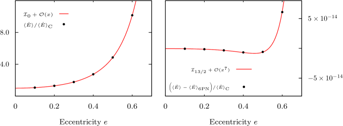
Figure 7: Agreement between numerical flux data and the 7PN expansion at smaller radius and larger eccentricities. An orbit with separation of $p=10^{3}$ was used. The left panel shows the energy flux as a function of eccentricity normalized to the circular-orbit limit (i.e., the curve closely resembles the Peters-Mathews enhancement function). The red curve shows the 7PN fit to this data. On the right, we subtract the fit (through 6PN order) from the energy flux data points. The residuals have dropped by 14 orders of magnitude. The residuals are then shown to still be well fit by the remaining 6.5PN and 7PN parts of the model even for $e=0.6$ .

Finally, at 7PN order there is a squared-log term and we again found the first two coefficients analytically

$$\mathcal{L}_{7L^{2}} =-\frac{1}{(1-e^{2})^{21/2}}\biggl{(}\frac{52525903}{617400}+\frac{8436767071}{740880}e^{2}+v_{4}e^{4}+v_{6}e^{6}+v_{8}e^{8}+\cdots\biggr{)}\qquad\qquad\qquad.$$ (111)

VI.4 Discussion

The analytic forms for the $e^{2}$ coefficients at the 5.5PN non-log, 6PN log, 6.5PN log, 7PN log, and 7PN log-squared orders were previously obtained by Johnson-McDaniel Johnson-McDaniel (2015). They are obtained by using the eccentric analogue of the simplification described in Johnson-McDaniel (2014) to predict leading logarithmic-type terms to all orders, starting from the expressions for the modes given in Appendix G of Mino et al. (1997).

Figure 8: Strong-field comparison between the 7PN expansion and energy fluxes computed with a Lorenz gauge/RWZ gauge hybrid self-force code Osburn et al. (2014) (courtesy T. Osburn).

The 7PN fit was obtained using orbits with eccentricities between $0.0$ and $0.1$, and using orbital separations of $p=10^{10}$ through $p=10^{35}$. A natural question to ask is how well does the PN expansion work if we compute fluxes from higher eccentricity orbits and from orbits with much smaller separations? The answer is: quite well. Fig. 7 shows (on the left) the circular orbit limit normalized energy flux (dominated by the Peters-Mathews term) as black points, and the red curve is the fit from our 7PN model. Here we have reduced the orbital separation to $p=10^{3}$ and we compare the data and model all the way up to $e=0.6$. On the right side we show the effect of subtracting the model containing all terms up to and including the 6PN contributions. With an orbit with a radius of $p=10^{3}$, the residuals have dropped by 14 orders of magnitude. The remaining part of the model (6.5PN and 7PN) is then shown to still fit these residuals.

We examined the fit then at still smaller radius orbits. Figure 8 compares our 7PN determination to energy fluxes obtained by T. Osburn using a Lorenz gauge/RWZ gauge hybrid code Osburn et al. (2014). Energy fluxes have accuracies of $10^{-3}$ all the way in as close as $p=30$.

VII Conclusions

In this paper we have presented a first set of results from a new eccentric-orbit MST code. The code, written in Mathematica, combines the MST formalism and arbitrary-precision functions to solve the perturbation equations to an accuracy of 200 digits. We computed the energy flux at infinity, at lowest order in the mass ratio (i.e., in the region of parameter space overlapped by BHP and PN theories). In this effort, we computed results for approximately 1,700 distinct orbits, with up to as many as 7,400 Fourier-harmonic modes per orbit.

The project had several principal new results. First, we confirmed previously computed PN flux expressions through 3PN order. Second, in the process of this analysis, we developed a procedure and new high-order series expansions for the non-closed form hereditary terms at 1.5PN, 2.5PN, and 3PN order. Significantly, at 2.5PN order we overcame some of the previous roadblocks to writing down accurate high-order expansions for this flux contribution (App. A). The 3PN hereditary term was shown to have a subtle singular behavior as $e_{t}\to 1$. All of this clarification of the behavior of the hereditary terms was aided by an asymptotic analysis of a set of enhancement functions. In the process we were able to predict the form of eccentricity singular factors that appear at each PN order. Third, based on that understanding, we then used the high accuracy of the code to find a mixture of new analytic and numeric flux terms between 3.5PN and 7PN. We built in expected forms for the eccentricity singular factors, allowing the determined power series in $e^{2}$ to better determine the flux at high values of $e$.

The code we have developed for this project can be used not only to compute fluxes but also local GSF quantities. Recently Akcay et al. Akcay et al. (2015) made comparisons between GSF and PN values of the eccentric orbit generalization of Detweiler’s redshift invariant ($\Delta U$) Detweiler (2008); Barack and Sago (2011). We may be able to extend these comparisons beyond the current 4PN level and compute currently unknown coefficients (in the linear in $\mu/M$ limit). We can also modify the code to make calculations on a Kerr background.

Appendix A The mass quadrupole tail at 1PN

In their Eqn. (5.14) Arun et al. Arun et al. (2008b) write the tail contribution to the mass quadrupole flux in terms of enhancement factors as

$$\begin{split}&\mathcal{F}_{\text{tail}}^{\text{mass quad}}=\frac{32}{5}\nu^{2}y^{13/2}\\ &\hskip 8.61108pt\times\left\{4\pi\varphi(e_{t})+\pi y\left[-\frac{428}{21}\alpha(e_{t})+\frac{178}{21}\nu\theta(e_{t})\right]\right\},\end{split}$$ (112)

where $\nu$ is the symmetric mass ratio. The $\alpha$ and $\theta$ enhancement factors contribute at 2.5PN and depend on the 1PN mass quadrupole. This dependence makes them more difficult to calculate than any of the other enhancement factors up to 3PN. Arun et al. outline a procedure for computing $\alpha$ and $\theta$ numerically, showing their results graphically.

In this appendix we summarize our calculation of the 2.5PN enhancement factor $\alpha$, which contributes to $\psi$ [see Arun et al. Eqn. (6.1a)]. Our presentation follows closely that given in Sec. IVD of Arun et al. Unlike them, we work in the $\mu/M\to 0$ limit and use the BHP notation already established in this paper. Significantly, we were able to find an analytic expression for $\alpha$ as a high-order power-series in eccentricity. We give this series (with a singular factor removed) to 20th-order in Sec. IV, but we have computed it to 70th order. Although we are working in the $\mu/M\to 0$ limit, it may be possible to employ the method outlined here to obtain the finite mass-ratio term $\theta$ in a similar power series.

A.1 Details of the flux calculation

With $y$ expanded in $p$ as discussed in the text, we are able to find 1PN expansions of $\mathcal{E}$ and $\mathcal{L}$ using Eqn. (22). In order to find the other orbital quantities that will go into the 1PN mass quadrupole we use the quasi-Keplerian (QK) parametrization Damour (1985). As that parametrization is well covered in Ref. Arun et al. (2008b) and many other papers we will not go into detail here, except to make two points.

First, in the QK parametrization $r_{p}$, $\varphi_{p}$ and their derivatives are expressed as functions of the eccentric anomaly $u$. As such, when computing the Fourier series coefficients of the mass quadrupole we perform integrations with respect to $u$. Additionally, we note that when using the QK parametrization, at 1PN there are 3 eccentricities $e_{t}$, $e_{r}$ and $e_{\varphi}$. Typically eccentric orbits are described using $e_{t}$. Through 3PN $e$ and $e_{t}$ are related to each other via (IV.4). We use this expression to convert known PN enhancement factors to $e$ dependence, as shown in Sec. IV.4.

To lowest order in $\mu/M$, the 1PN mass quadrupole is given by

$$\begin{split}I_{ij}&=\mu\bigg{[}\left(1+\frac{29}{42}\dot{x}_{p}^{2}-\frac{5}{7}\frac{M}{r_{p}}\right)x_{p}^{\langle i}x_{p}^{j\rangle}\\ &\hskip 60.27759pt+\frac{11}{21}r_{p}^{2}\dot{x}_{p}^{\langle i}\dot{x}_{p}^{j\rangle}-\frac{4}{7}r_{p}\dot{r}_{p}x_{p}^{\langle i}\dot{x}_{p}^{j\rangle}\bigg{]},\end{split}$$ (113)

with the angle brackets indicating a symmetric trace free projection (e.g. $x_{p}^{\langle i}x_{p}^{j\rangle}=x_{p}^{i}x_{p}^{j}-r_{p}^{2}\delta^{ij}/3$). We start by expanding $I_{ij}$ in a Fourier series

$$I_{ij}(t)=\sum_{n=-\infty}^{\infty}\sum_{m=-2}^{2}\underset{(m,n)\ }{\mathcal{I}_{ij}}\ e^{i\omega_{mn}t}.$$ (114)

Note that in this series we are following the sign convention of Arun et al. which differs from that in, e.g. Eqn. (30). Arun et al. give the mass quadrupole tail flux in their Eqn. (4.17) as

$$\mathcal{F}_{\text{tail}}^{\text{mass quad}}=$$ (115)

$$\frac{4M}{5}\left\langle I_{ij}^{(3)}(t)\int_{0}^{\infty}d\tau I_{ij}^{(5)}(t-\tau)\left[\log\left(\frac{\tau}{2r_{0}}\right)+\frac{11}{12}\right]\right\rangle.$$

Here the superscripts (3) and (5) indicate the number of time derivatives, and $r_{0}$ is a constant with dimensions length which does not appear in the final expression for the flux. Inserting Eqn. (114) we find

$$\mathcal{F}_{\text{tail}}^{\text{mass quad}}=-\frac{4M}{5}\sum_{m,m^{\prime},n,n^{\prime}}\omega_{mn}^{3}\omega_{m^{\prime}n^{\prime}}^{5}$$ (116)

$$\hskip 34.44434pt\times\underset{(m,n)\ }{\mathcal{I}_{ij}}\underset{(m^{\prime},n^{\prime})\ }{\mathcal{I}^{*}_{ij}}\left\langle e^{i\left[\Omega_{\varphi}(m-m^{\prime})+\Omega_{r}(n-n^{\prime})\right]t}\right\rangle$$

$$\hskip 34.44434pt\times\int_{0}^{\infty}d\tau\ e^{i\omega_{m^{\prime}n^{\prime}}\tau}\left[\log\left(\frac{\tau}{2r_{0}}\right)+\frac{11}{12}\right].$$

In deriving Eqn. (116) we have reversed the sign on both $m^{\prime}$ and $n^{\prime}$ and used the crossing relation ${}_{(m,n)}\mathcal{I}_{ij}={{}_{(-m,-n)}\mathcal{I}^{*}_{ij}}$. We split this expression up into four terms, writing

$$\mathcal{F}_{\text{tail}}^{\text{mass quad}}=\sum_{n,n^{\prime},m,m^{\prime}}\mathcal{A}\cdot\mathcal{B}\cdot\mathcal{C}\cdot\mathcal{D},$$ (117)

with

$$\begin{split}\mathcal{A}&=-\frac{4M}{5}\omega_{mn}^{3}\omega_{m^{\prime}n^{\prime}}^{5},\\ \mathcal{B}&=\underset{(m,n)\ }{\mathcal{I}_{ij}}\underset{(m^{\prime},n^{\prime})\ }{\mathcal{I}^{*}_{ij}},\\ \mathcal{C}&=\left\langle e^{i\left[\Omega_{\varphi}(m-m^{\prime})+\Omega_{r}(n-n^{\prime})\right]t}\right\rangle,\\ \mathcal{D}&=\int_{0}^{\infty}d\tau\ e^{i\omega_{m^{\prime}n^{\prime}}\tau}\left[\log\left(\frac{\tau}{2r_{0}}\right)+\frac{11}{12}\right].\end{split}$$ (118)

Each of these terms has 0PN and 1PN contributions. For example, $\mathcal{A}=\mathcal{A}_{0}+y\mathcal{A}_{1}$, and similarly for $\mathcal{B}$, $\mathcal{C}$, and $\mathcal{D}$. Then, through 1PN the summand in Eqn. (117) is

$$\mathcal{A}\cdot\mathcal{B}\cdot\mathcal{C}\cdot\mathcal{D} =\mathcal{A}_{0}\mathcal{B}_{0}\mathcal{C}_{0}\mathcal{D}_{0}+y\bigg{(}\mathcal{A}_{1}\mathcal{B}_{0}\mathcal{C}_{0}\mathcal{D}_{0}$$ (119)

$$+\mathcal{A}_{0}\mathcal{B}_{1}\mathcal{C}_{0}\mathcal{D}_{0}+\mathcal{A}_{0}\mathcal{B}_{0}\mathcal{C}_{1}\mathcal{D}_{0}+\mathcal{A}_{0}\mathcal{B}_{0}\mathcal{C}_{0}\mathcal{D}_{1}\bigg{)}.$$

Expanding $\mathcal{A}$ we find

$$\begin{split}\mathcal{A}_{0}&=-\frac{4y^{12}}{5M^{7}}n^{3}n^{\prime 5},\\ \mathcal{A}_{1}&=-\frac{12y^{12}}{5M^{7}}\frac{\left(3mn^{2}n^{\prime 5}+5m^{\prime}n^{3}n^{\prime 4}-8n^{3}n^{\prime 5}\right)}{1-e_{t}^{2}}\end{split}$$ (120)

We next consider the moments in $\mathcal{B}$, writing

$$\underset{(m,n)\ }{\mathcal{I}_{ij}}=\underset{(m,n)\ }{\mathcal{I}_{ij}^{0}}+y\underset{(m,n)\ }{\mathcal{I}_{ij}^{1}},$$ (121)

and hence

$$\begin{split}\mathcal{B}_{0}&=\underset{(m,n)\ }{\mathcal{I}_{ij}^{0}}\underset{(m^{\prime},n^{\prime})\ }{\mathcal{I}_{ij}^{0*}},\\ \mathcal{B}_{1}&=\underset{(m,n)\ }{\mathcal{I}_{ij}^{0}}\underset{(m^{\prime},n^{\prime})\ }{\mathcal{I}_{ij}^{1*}}+\underset{(m,n)\ }{\mathcal{I}_{ij}^{1}}\underset{(m^{\prime},n^{\prime})\ }{\mathcal{I}_{ij}^{0*}}.\end{split}$$ (122)

The heart of the calculation of $\alpha$ comes down to computing the Fourier coefficients ${}_{(m,n)}{\mathcal{I}_{ij}^{1}}$ in Eqn. (122). As mentioned above, we compute these terms by representing the elements of $I_{ij}$ in the QK parametrization. The Fourier coefficients are then computed by integrating with respect to the eccentric anomaly $u$. While we cannot perform these integrals for completely generic expressions, we do find that we can expand $I_{ij}$ in eccentricity and obtain ${}_{(m,n)}{\mathcal{I}_{ij}^{1}}$ as a power series in $e_{t}$. Furthermore, as shown in Sec. IV we are able to remove singular factors in this expansion, leading to much improved convergence for large eccentricity. Significantly, we find that $\mathcal{B}_{0}$ and $\mathcal{B}_{1}$ are only nonzero when $m=m^{\prime}$.

Next we consider $\mathcal{C}$. Expanding the complex exponential to 1PN, we can perform the time-average integral and we find

$$\begin{split}\mathcal{C}_{0}&=\delta_{n,n^{\prime}},\\ \mathcal{C}_{1}&=i\pi(m-m^{\prime})\delta_{n,n^{\prime}}+\frac{m-m^{\prime}}{n-n^{\prime}}\left(1-\delta_{n,n^{\prime}}\right),\end{split}$$ (123)

where the $1-\delta_{n,n^{\prime}}$ indicates that the second term vanishes when $n=n^{\prime}$. The case where we employ $\mathcal{C}_{0}=\delta_{n,n^{\prime}}$ greatly simplifies the calculation, taking us from a doubly-infinite sum to a singly-infinite sum. Remarkably, the $\mathcal{C}_{1}$ term does not contribute at all. This follows from the fact that it is proportional to $m-m^{\prime}$ and the $B_{0}$ terms only contribute when $m=m^{\prime}$. Thus, the doubly-infinite sum found by Arun et al. reduces to a singly-infinite sum (at least) in the limit that $\mu/M\to 0$ at 1PN.

The tail integral for $\mathcal{D}$ is computed using expressions in Ref. Arun et al. (2008b). Each of the terms $\mathcal{D}_{0}$ and $\mathcal{D}_{1}$ is complex and we find that the imaginary part cancels after summing over positive and negative $m^{\prime}$ and $n^{\prime}$, leaving a purely real contribution to the flux. The real contributions to these terms are

$$\mathcal{D}_{0}=-\frac{M}{y^{3/2}}\frac{\pi}{2|n^{\prime}|},\quad\mathcal{D}_{1}=\frac{3\pi M(n^{\prime}-m^{\prime})}{2y^{3/2}(1-e_{t}^{2})n^{\prime}|n^{\prime}|}.$$ (124)

At this point we combine the 0PN and 1PN contributions to $\mathcal{A}$, $\mathcal{B}$, $\mathcal{C}$, and $\mathcal{D}$ in Eqns. (119) and (117). The Kronecker deltas in Eqn. (123) along with the fact that $\mathcal{B}$ is nonzero only for $m=m^{\prime}$ reduces the sum to

$$\mathcal{F}_{\text{tail}}^{\text{mass quad}}=\sum_{n=-\infty}^{\infty}\sum_{m=-2}^{2}\mathcal{A}\cdot\mathcal{B}\cdot\mathcal{C}\cdot\mathcal{D}.$$ (125)

Furthermore, expanding the Fourier coefficients ${}_{(m,n)}{\mathcal{I}_{ij}^{1}}$ in eccentricity to some finite order truncates the sum over $n$. This sum yields both the 1.5PN enhancement factor $\varphi$ and the 2.5PN factor $\alpha$.

Appendix B Solving for $\nu$

The full forms of the $\alpha_{n}^{\nu}$, $\beta_{n}^{\nu}$, and $\gamma_{n}^{\nu}$ mentioned in II.2.1 are

$$\alpha_{n}^{\nu} =\frac{i\epsilon\kappa(n+\nu+1+s+i\epsilon)}{(n+\nu+1)(2n+2\nu+3)}$$

$$\times(n+\nu+1+s-i\epsilon)(n+\nu+1+i\tau),$$

$$\beta_{n}^{\nu} =-\lambda-s(s+1)+(n+\nu)(n+\nu+1)+\epsilon^{2}+\epsilon(\epsilon-mq)$$

$$+\frac{\epsilon(\epsilon-mq)(s^{2}+\epsilon^{2})}{(n+\nu)(n+\nu+1)},$$

$$\gamma_{n}^{\nu} =-\frac{i\epsilon\kappa(n+\nu-s+i\epsilon)(n+\nu-s-i\epsilon)(n+\nu-i\tau)}{(n+\nu)(2n+2\nu-1)}.$$ (126)

Now introduce the continued fractions

$$R_{n}^{\nu}\equiv\frac{a_{n}^{\nu}}{a_{n-1}^{\nu}}=-\frac{\gamma_{n}^{\nu}}{\beta_{n}^{\nu}-}\frac{\alpha_{n}^{\nu}\gamma_{n+1}^{\nu}}{\beta_{n+1}^{\nu}-}\frac{\alpha_{n+1}^{\nu}\gamma_{n+2}^{\nu}}{\beta_{n+2}^{\nu}-}\cdots,$$

$$L_{n}^{\nu}\equiv\frac{a_{n}^{\nu}}{a_{n+1}^{\nu}}=-\frac{\alpha_{n}^{\nu}}{\beta_{n}^{\nu}-}\frac{\alpha_{n-1}^{\nu}\gamma_{n}^{\nu}}{\beta_{n-1}^{\nu}-}\frac{\alpha_{n-2}^{\nu}\gamma_{n-1}^{\nu}}{\beta_{n-2}^{\nu}-}\cdots.$$ (127)

Then recall that the series coefficients $\{a_{n}^{\nu}\}$ satisfy the three-term recurrence (10), which can now be rewritten as

$$\beta_{n}^{\nu}+\alpha_{n}^{\nu}R_{n+1}+\gamma_{n}^{\nu}L_{n-1}=0.$$ (128)

This holds for arbitrary $n$, so in particular we can set $n=0$,

$$\beta_{0}^{\nu}+\alpha_{0}^{\nu}R_{1}+\gamma_{0}^{\nu}L_{-1}=0.$$ (129)

In practice, $\nu$ is determined by numerically looking for the roots of (129). Formally, $R_{n}^{\nu}$ and $L_{n}^{\nu}$ have an infinite depth, but may be truncated at finite depth in (129) depending on the precision to which it is necessary to determine $\nu$.

We note also that there exists a low-frequency expansion for $\nu$. Letting $\epsilon=2M\omega$,

$$\nu= l+\frac{1}{2l+1}\bigg{(}-2-\frac{s^{2}}{l(l+1)}+\frac{\left[(l+1)^{2}-s^{2}\right]^{2}}{(2l+1)(2l+2)(2l+3)}$$

$$-\frac{(l^{2}-s^{2})^{2}}{(2l-1)(2l)(2l+1)}\bigg{)}\epsilon^{2}+\mathcal{O}(\epsilon^{4}).$$

For given $l$, we are able to take this expansion to arbitrary order, and therefore easily and quickly determine $\nu$ to very high precision for small frequencies.

Appendix C Analytic and numeric coefficients in the high-order post-Newtonian functions

Numerical values for the remaining coefficients in the high-order PN functions (95)-(111) are provided in Tables 1-15.

Table 1: Coefficients in the 3.5PN function according to the form of Eqn. (95) for which we were unable to determine rational forms.

3.5PN Coefficients
Coefficient	Decimal Form
$b_{26}$	$-1.490561574783877$
$b_{28}$	$-1.193065651880562$
$b_{30}$	$-0.9727274285773439$
$b_{32}$	$-0.8055449753687710$
$b_{34}$	$-0.6760669725730609$
$b_{36}$	$-0.5740065189983486$
$b_{38}$	$-0.4923153284656641$
$b_{40}$	$-0.4260425626411813$
$b_{42}$	$-0.3716342707794599$
$b_{44}$	$-0.3264898836852403$
$b_{46}$	$-0.2886737566317485$
$b_{48}$	$-0.2567230158706580$
$b_{50}$	$-0.229516796538214$
$b_{52}$	$-0.2061855361551$
$b_{54}$	$-0.1860469549$

Table 2: Coefficients in the 4PN non-log function $\mathcal{L}_{4}$ according to the form of Eqn. (96).

4PN Non-Log Coefficients
Coefficient	Decimal Form
$d_{8}$	-12385.51003537713
$d_{10}$	5863.111480566811
$d_{12}$	3622.327433443339
$d_{14}$	2553.863176036157
$d_{16}$	2026.951300184891
$d_{18}$	1688.454045610002
$d_{20}$	1449.705886053665
$d_{22}$	1271.358072870572
$d_{24}$	1132.705339539895
$d_{26}$	1021.659868559411
$d_{28}$	930.6413570026334
$d_{30}$	854.6360714818981
$d_{32}$	790.1870990544641
$d_{34}$	734.8297131797
$d_{36}$	686.7572696
$d_{38}$	644.61426
$d_{40}$	607.363

Table 3: Coefficients in the 4.5PN non-log function $\mathcal{L}_{9/2}$ according to the form of Eqn. (98).

4.5PN Non-Log Coefficients
Coefficient	Decimal Form
$h_{4}$	$34992.49298556799$
$h_{6}$	$39847.21900599596$
$h_{8}$	$-6749.004994216654$
$h_{10}$	$-11556.5757682355$
$h_{12}$	$-3380.99341129105$
$h_{14}$	$-2106.48821413306$
$h_{16}$	$-1605.13441975986$
$h_{18}$	$-1305.76892323295$
$h_{20}$	$-1104.20944659088$
$h_{22}$	$-958.287100012754$
$h_{24}$	$-847.360081662457$
$h_{26}$	$-759.987768729771$
$h_{28}$	$-689.280637106089$
$h_{30}$	$-630.824342070861$
$h_{32}$	$-581.651645011457$
$h_{34}$	$-539.69025201625$
$h_{36}$	$-503.44686180$

Table 4: Coefficients in the 4.5PN log function $\mathcal{L}_{9/2L}$ according to the form of Eqn. (99).

4.5PN Log Coefficients
Coefficient	Decimal Form
$g_{20}$	$0.00005237112441246353$
$g_{22}$	$1.500221637093169\times 10^{-6}$
$g_{24}$	$-1.445846088397795\times 10^{-6}$
$g_{26}$	$-3.761668215289038\times 10^{-7}$
$g_{28}$	$-6.09085540489931\times 10^{-8}$
$g_{30}$	$-8.1161948669\times 10^{-9}$

Table 5: Coefficients in the 5PN non-log function $\mathcal{L}_{5}$ according to the form of equation Eqn. (100).

5PN Non-Log Coefficients
Coefficient	Decimal Form
$k_{2}$	$-30239.82434287415$
$k_{4}$	$-104593.9352475713$
$k_{6}$	$75463.00111171990$
$k_{8}$	$269065.9776584819$
$k_{10}$	$73605.36477482046$
$k_{12}$	$-41367.54579072399$
$k_{14}$	$-30242.01469796259$
$k_{16}$	$-22936.05821746133$
$k_{18}$	$-18706.03853031426$
$k_{20}$	$-15829.44370858490$
$k_{22}$	$-13730.52183792896$
$k_{24}$	$-12127.0027508276$
$k_{26}$	$-10860.422505$

Table 6: Coefficients in the 5PN log function $\mathcal{L}_{5L}$ according to the form of Eqn. (101).

5PN Log Coefficients
Coefficient	Decimal Form
$j_{26}$	$-17.11762038204405$
$j_{28}$	$-13.5361663264$

Table 7: Coefficients in the 5.5PN non-log function $\mathcal{L}_{11/2}$ according to the form of Eqn. (102).

5.5PN Non-Log Coefficients
Coefficient	Decimal Form
$m_{2}$	$-6745.196131429910$
$m_{4}$	$-141316.5392653812$
$m_{6}$	$-469215.6608702663$
$m_{8}$	$-434086.0636932912$
$m_{10}$	$48474.32085716919$
$m_{12}$	$129328.2556268356$
$m_{14}$	$72095.03819665170$
$m_{16}$	$53240.504083351$
$m_{18}$	$42978.60994$

Table 8: Coefficients in the 5.5PN log function $\mathcal{L}_{11/2L}$ according to the form of Eqn. (103).

5.5PN Log Coefficients
Coefficient	Decimal Form
$l_{12}$	$189.3698825402159$
$l_{14}$	$0.007977195397456623$
$l_{16}$	$0.0239041225377$

Table 9: Coefficients in the 6PN non-log function $\mathcal{L}_{6}$ according to the form of Eqn. (104).

6PN Non-Log Coefficients
Coefficient	Decimal Form
$n_{2}$	$183747.5626219038$
$n_{4}$	$1960389.869256877$
$n_{6}$	$5197796.234905070$
$n_{8}$	$2705571.654688992$
$n_{10}$	$-1438997.974016927$
$n_{12}$	$-923762.260160$

Table 10: Coefficients in the 6PN log function $\mathcal{L}_{6L}$ according to the form of Eqn. (105).

6PN Log Coefficients
Coefficient	Decimal Form
$p_{2}$	$-45332.65954460482$
$p_{4}$	$-339065.8391750689$
$p_{6}$	$-612772.4442656394$
$p_{8}$	$-63054.18877810686$
$p_{10}$	$298247.27730847$
$p_{12}$	$107300.427923$

Table 11: Coefficients in the 6.5PN non-log function $\mathcal{L}_{13/2}$ according to the form of Eqn. (107).

6.5PN Non-Log Coefficients
Coefficient	Decimal Form
$r_{2}$	$-127378.8277728414$
$r_{4}$	$-1087743.1117750650$
$r_{6}$	$-1820396.3219686398$
$r_{8}$	$837531.195260$
$r_{10}$	$2191527.42$
$r_{12}$	$-676000$

Table 12: Coefficients in the 6.5PN log function $\mathcal{L}_{13/2L}$ according to the form of Eqn. (108).

6.5PN Log Coefficients
Coefficient	Decimal Form
$s_{2}$	$3556.505482510765$
$s_{4}$	$-88650.24536994091$
$s_{6}$	$-725275.3694386568$
$s_{8}$	$-1383744.78113972$
$s_{10}$	$-775068.8299$
$s_{12}$	$-117673$

Table 13: Coefficients in the 7PN non-log function $\mathcal{L}_{7}$ according to the form of Eqn. (109).

7PN Non-Log Coefficients
Coefficient	Decimal Form
$t_{2}$	$274599.5315289643$
$t_{4}$	$-1830774.789990$
$t_{6}$	$-22622781.31$

Table 14: Coefficients in the 7PN log function $\mathcal{L}_{7L}$ according to the form of Eqn. (110).

7PN Log Coefficients
Coefficient	Decimal Form
$u_{2}$	$196177.8173496888$
$u_{4}$	$3290034.8114615$
$u_{6}$	$13274887.225$
$u_{8}$	$17171440$

Table 15: Coefficients in the 7PN log-squared function $\mathcal{L}_{7L^{2}}$ according to the form of Eqn. (111).

7PN Log-Squared Coefficients
Coefficient	Decimal Form
$v_{2}$	$11387.49469684699$
$v_{4}$	$157165.280283919$
$v_{6}$	$568228.86246$
$v_{8}$	$677671.2$

References

- (1) “Ligo home page,” http://www.ligo.caltech.edu/.
- (2) “Virgo homepage,” https://www.virgo-gw.eu/.
- (3) “KAGRA home page,” http://gwcenter.icrr.u-tokyo.ac.jp/en/.
- (4) “elisa science home page,” http://www.elisascience.org/.
- Abbott et al. (2016) B. P. Abbott, R. Abbott, T. D. Abbott, M. R. Abernathy, F. Acernese, K. Ackley, C. Adams, T. Adams, P. Addesso, R. X. Adhikari, and et al., Physical Review Letters 116, 061102 (2016), arXiv:1602.03837 [gr-qc] .
- Le Tiec (2014) A. Le Tiec, International Journal of Modern Physics D 23, 1430022 (2014), arXiv:1408.5505 [gr-qc] .
- Baumgarte and Shapiro (2010) T. W. Baumgarte and S. L. Shapiro, Numerical Relativity: Solving Einstein’s Equations on the Computer (Cambridge University Press, 2010).
- Lehner and Pretorius (2014) L. Lehner and F. Pretorius, Annu. Rev. Astron. Astrophys. 52, 661 (2014), arXiv:1405.4840 [astro-ph.HE] .
- Will (2011) C. M. Will, Proceedings of the National Academy of Science 108, 5938 (2011), arXiv:1102.5192 [gr-qc] .
- Blanchet (2014) L. Blanchet, Living Reviews in Relativity 17, 2 (2014), arXiv:1310.1528 [gr-qc] .
- Drasco and Hughes (2004) S. Drasco and S. A. Hughes, Phys. Rev. D 69, 044015 (2004).
- Barack (2009) L. Barack, Class. Quant. Grav. 26, 213001 (2009), arXiv:0908.1664 [gr-qc] .
- Poisson et al. (2011) E. Poisson, A. Pound, and I. Vega, Living Rev. Rel. 14, 7 (2011), arXiv:gr-qc/1102.0529 .
- Thornburg (2011) J. Thornburg, GW Notes, Vol. 5, p. 3-53 5, 3 (2011), arXiv:1102.2857 [gr-qc] .
- Buonanno and Damour (1999) A. Buonanno and T. Damour, Phys. Rev. D 59, 084006 (1999), gr-qc/9811091 .
- Buonanno et al. (2009) A. Buonanno, Y. Pan, H. P. Pfeiffer, M. A. Scheel, L. T. Buchman, and L. E. Kidder, Phys. Rev. D 79, 124028 (2009), arXiv:0902.0790 [gr-qc] .
- Damour (2010) T. Damour, Phys. Rev. D 81, 024017 (2010), arXiv:0910.5533 [gr-qc] .
- Hinderer et al. (2013) T. Hinderer, A. Buonanno, A. H. Mroué, D. A. Hemberger, G. Lovelace, H. P. Pfeiffer, L. E. Kidder, M. A. Scheel, B. Szilagyi, N. W. Taylor, and S. A. Teukolsky, Phys. Rev. D 88, 084005 (2013), arXiv:1309.0544 [gr-qc] .
- Damour (2013) T. Damour, ArXiv e-prints (2013), arXiv:1312.3505 [gr-qc] .
- Taracchini et al. (2014) A. Taracchini, A. Buonanno, Y. Pan, T. Hinderer, M. Boyle, D. A. Hemberger, L. E. Kidder, G. Lovelace, A. H. Mroué, H. P. Pfeiffer, M. A. Scheel, B. Szilágyi, N. W. Taylor, and A. Zenginoglu, Phys. Rev. D 89, 061502 (2014), arXiv:1311.2544 [gr-qc] .
- Detweiler (2008) S. Detweiler, Phys. Rev. D 77, 124026 (2008), arXiv:0804.3529 [gr-qc] .
- Sago et al. (2008) N. Sago, L. Barack, and S. L. Detweiler, Phys. Rev. D 78, 124024 (2008), arXiv:0810.2530 [gr-qc] .
- Barack and Sago (2009) L. Barack and N. Sago, Phys. Rev. Lett. 102, 191101 (2009), arXiv:0902.0573 [gr-qc] .
- Blanchet et al. (2010a) L. Blanchet, S. Detweiler, A. Le Tiec, and B. F. Whiting, Phys. Rev. D 81, 064004 (2010a), arXiv:0910.0207 [gr-qc] .
- Blanchet et al. (2010b) L. Blanchet, S. Detweiler, A. Le Tiec, and B. F. Whiting, Phys. Rev. D 81, 084033 (2010b), arXiv:1002.0726 [gr-qc] .
- Fujita (2012) R. Fujita, Progress of Theoretical Physics 128, 971 (2012), arXiv:1211.5535 [gr-qc] .
- Shah et al. (2014) A. G. Shah, J. L. Friedman, and B. F. Whiting, Phys. Rev. D 89, 064042 (2014), arXiv:1312.1952 [gr-qc] .
- Shah (2014a) A. G. Shah, Phys. Rev. D 90, 044025 (2014a), arXiv:1403.2697 [gr-qc] .
- Johnson-McDaniel et al. (2015) N. K. Johnson-McDaniel, A. G. Shah, and B. F. Whiting, Phys. Rev. D 92, 044007 (2015), arXiv:1503.02638 [gr-qc] .
- Akcay et al. (2015) S. Akcay, A. Le Tiec, L. Barack, N. Sago, and N. Warburton, Phys. Rev. D 91, 124014 (2015), arXiv:1503.01374 [gr-qc] .
- Poisson (1993) E. Poisson, Phys. Rev. D 47, 1497 (1993).
- Cutler et al. (1993) C. Cutler, L. S. Finn, E. Poisson, and G. J. Sussman, Phys. Rev. D 47, 1511 (1993).
- Tagoshi and Sasaki (1994) H. Tagoshi and M. Sasaki, Progress of Theoretical Physics 92, 745 (1994), gr-qc/9405062 .
- Tagoshi and Nakamura (1994) H. Tagoshi and T. Nakamura, Phys. Rev. D 49, 4016 (1994).
- Poisson and Sasaki (1995) E. Poisson and M. Sasaki, Phys. Rev. D 51, 5753 (1995), gr-qc/9412027 .
- Tanaka et al. (1993) T. Tanaka, M. Shibata, M. Sasaki, H. Tagoshi, and T. Nakamura, Progress of Theoretical Physics 90, 65 (1993).
- Apostolatos et al. (1993) T. Apostolatos, D. Kennefick, A. Ori, and E. Poisson, Phys. Rev. D 47, 5376 (1993).
- Cutler et al. (1994) C. Cutler, D. Kennefick, and E. Poisson, Phys. Rev. D 50, 3816 (1994).
- Tagoshi (1995) H. Tagoshi, Progress of Theoretical Physics 93, 307 (1995).
- Dolan et al. (2015) S. R. Dolan, P. Nolan, A. C. Ottewill, N. Warburton, and B. Wardell, Phys. Rev. D 91, 023009 (2015), arXiv:1406.4890 [gr-qc] .
- Bini et al. (2015) D. Bini, T. Damour, and A. Geralico, (2015), arXiv:1511.04533 [gr-qc] .
- Hopper et al. (2015) S. Hopper, C. Kavanagh, and A. C. Ottewill, ArXiv e-prints (2015), arXiv:1512.01556 [gr-qc] .
- Amaro-Seoane et al. (2007) P. Amaro-Seoane, J. R. Gair, M. Freitag, M. C. Miller, I. Mandel, C. J. Cutler, and S. Babak, Class. Quant. Grav. 24, R113 (2007), arXiv:astro-ph/0703495 .
- Amaro-Seoane et al. (2014) P. Amaro-Seoane, J. R. Gair, A. Pound, S. A. Hughes, and C. F. Sopuerta, ArXiv e-prints (2014), arXiv:1410.0958 .
- Hopman and Alexander (2005) C. Hopman and T. Alexander, Astrophysical Journal 629, 362 (2005), arXiv:astro-ph/0503672 .
- Miller and Colbert (2004) M. C. Miller and E. J. M. Colbert, International Journal of Modern Physics D 13, 1 (2004).
- Brown et al. (2007) D. A. Brown, J. Brink, H. Fang, J. R. Gair, C. Li, G. Lovelace, I. Mandel, and K. S. Thorne, Physical Review Letters 99, 201102 (2007), gr-qc/0612060 .
- Arun et al. (2008a) K. G. Arun, L. Blanchet, B. R. Iyer, and M. S. S. Qusailah, Phys. Rev. D 77, 064034 (2008a), arXiv:0711.0250 [gr-qc] .
- Arun et al. (2008b) K. G. Arun, L. Blanchet, B. R. Iyer, and M. S. S. Qusailah, Phys. Rev. D 77, 064035 (2008b), arXiv:0711.0302 [gr-qc] .
- Arun et al. (2009) K. G. Arun, L. Blanchet, B. R. Iyer, and S. Sinha, Phys. Rev. D 80, 124018 (2009), arXiv:0908.3854 [gr-qc] .
- Sasaki and Tagoshi (2003) M. Sasaki and H. Tagoshi, Living Reviews in Relativity 6, 6 (2003), gr-qc/0306120 .
- Sago and Fujita (2015) N. Sago and R. Fujita, Progress of Theoretical and Experimental Physics 2015, 073E03 (2015), arXiv:1505.01600 [gr-qc] .
- Mano et al. (1996a) S. Mano, H. Suzuki, and E. Takasugi, Progress of Theoretical Physics 96, 549 (1996a), gr-qc/9605057 .
- Mano et al. (1996b) S. Mano, H. Suzuki, and E. Takasugi, Progress of Theoretical Physics 95, 1079 (1996b), gr-qc/9603020 .
- Hopper and Evans (2010) S. Hopper and C. R. Evans, Phys. Rev. D 82, 084010 (2010).
- Hopper et al. (2015) S. Hopper, E. Forseth, T. Osburn, and C. R. Evans, Phys. Rev. D 92, 044048 (2015), arXiv:1506.04742 [gr-qc] .
- Misner et al. (1973) C. Misner, K. Thorne, and J. Wheeler, Gravitation (Freeman, San Francisco, CA, U.S.A., 1973).
- Martel and Poisson (2005) K. Martel and E. Poisson, Phys. Rev. D 71, 104003 (2005), arXiv:gr-qc/0502028 .
- Teukolsky (1973) S. Teukolsky, Astrophys. J. 185, 635 (1973).
- Newman and Penrose (1962) E. Newman and R. Penrose, Journal of Mathematical Physics 3, 566 (1962).
- Newman and Penrose (1963) E. Newman and R. Penrose, Journal of Mathematical Physics 4, 998 (1963).
- Kinnersley (1969) W. Kinnersley, Journal of Mathematical Physics 10, 1195 (1969).
- Bardeen and Press (1973) J. M. Bardeen and W. H. Press, Journal of Mathematical Physics 14, 7 (1973).
- Leaver (1986) E. W. Leaver, Journal of Mathematical Physics 27, 1238 (1986).
- Shah (2014b) A. G. Shah (private communication, 2014).
- Chandrasekhar (1975) S. Chandrasekhar, Royal Society of London Proceedings Series A 343, 289 (1975).
- Chandrasekhar and Detweiler (1975) S. Chandrasekhar and S. Detweiler, Royal Society of London Proceedings Series A 345, 145 (1975).
- Chandrasekhar (1983) S. Chandrasekhar, The Mathematical Theory of Black Holes, The International Series of Monographs on Physics, Vol. 69 (Clarendon, Oxford, 1983).
- Berndston (2007) M. Berndston, Harmonic Gauge Perturbations of the Schwarzschild Metric, Ph.D. thesis, University of Colorado (2007), arXiv:0904.0033v1 .
- Barack and Sago (2010) L. Barack and N. Sago, Phys. Rev. D 81, 084021 (2010), arXiv:1002.2386 [gr-qc] .
- Darwin (1959) C. Darwin, Proc. R. Soc. Lond. A 249, 180 (1959).
- Gradshteyn et al. (2007) I. S. Gradshteyn, I. M. Ryzhik, A. Jeffrey, and D. Zwillinger, Table of Integrals, Series, and Products, Seventh Edition by I. S. Gradshteyn, I. M. Ryzhik, Alan Jeffrey, and Daniel Zwillinger. Elsevier Academic Press, 2007. ISBN 012-373637-4 (2007).
- Barack et al. (2008) L. Barack, A. Ori, and N. Sago, Phys. Rev. D 78, 084021 (2008), arXiv:0808.2315 .
- Damour (1985) D. N. Damour, T., Annales de l’institut Henri Poincaré (A) Physique théorique 43, 107 (1985).
- Königsdörffer and Gopakumar (2005) C. Königsdörffer and A. Gopakumar, Phys. Rev. D 71, 024039 (2005), gr-qc/0501011 .
- Königsdörffer and Gopakumar (2006) C. Königsdörffer and A. Gopakumar, Phys. Rev. D 73, 124012 (2006), gr-qc/0603056 .
- Gopakumar and Schäfer (2011) A. Gopakumar and G. Schäfer, Phys. Rev. D 84, 124007 (2011).
- Peters and Mathews (1963) P. C. Peters and J. Mathews, Physical Review 131, 435 (1963).
- Blanchet and Schafer (1993) L. Blanchet and G. Schafer, Classical and Quantum Gravity 10, 2699 (1993).
- Wiseman (1993) A. G. Wiseman, Phys. Rev. D 48, 4757 (1993).
- Maggiore (2007) M. Maggiore, Gravitational Waves: Volume 1: Theory and Experiments, Gravitational Waves (OUP Oxford, 2007).
- Forseth (2014) E. Forseth (2014) , Talk presented at the 17th Capra meeting held at Caltech, http://www.tapir.caltech.edu/~capra17/Schedule.shtml.
- Forseth (2015) E. Forseth (2015) , Talk presented at the APS April meeting held in Baltimore, MD, http://meetings.aps.org/Meeting/APR15/Session/X13.2.
- Evans (2015) C. Evans (2015) , Talk presented at the 18th Capra meeting held at Yukawa Institute for Theoretical Physics, Kyoto University, Kyoto, Japan, http://www2.yukawa.kyoto-u.ac.jp/~capra18/Charles_Evans.pdf.
- Abramowitz and Stegun (1972) M. Abramowitz and I. A. Stegun, Handbook of Mathematical Functions, New York: Dover, 1972 (1972).
- (86) DLMF, “NIST Digital Library of Mathematical Functions,” http://dlmf.nist.gov/, Release 1.0.10 of 2015-08-07, online companion to Olver et al. (2010a).
- Olver et al. (2010a) F. W. J. Olver, D. W. Lozier, R. F. Boisvert, and C. W. Clark, eds., NIST Handbook of Mathematical Functions (Cambridge University Press, New York, NY, 2010) print companion to DLMF .
- Loutrel and Yunes (2016) N. Loutrel and N. Yunes (private communication, 2016).
- Kavanagh et al. (2015) C. Kavanagh, A. C. Ottewill, and B. Wardell, Phys. Rev. D92, 084025 (2015), arXiv:1503.02334 [gr-qc] .
- Johnson-McDaniel (2015) N. K. Johnson-McDaniel (private communication, 2015).
- Johnson-McDaniel (2014) N. K. Johnson-McDaniel, Phys. Rev. D 90, 024043 (2014), arXiv:1405.1572 [gr-qc] .
- Mino et al. (1997) Y. Mino, M. Sasaki, M. Shibata, H. Tagoshi, and T. Tanaka, Progress of Theoretical Physics Supplement 128, 1 (1997), gr-qc/9712057 .
- Osburn et al. (2014) T. Osburn, E. Forseth, C. R. Evans, and S. Hopper, Phys. Rev. D 90, 104031 (2014).
- Barack and Sago (2011) L. Barack and N. Sago, Phys. Rev. D 83, 084023 (2011), arXiv:1101.3331 [gr-qc] .
- Olver et al. (2010b) F. W. J. Olver, D. W. Lozier, R. F. Boisvert, and C. W. Clark, eds., NIST Handbook of Mathematical Functions (Cambridge University Press, New York, NY, 2010) print companion to DLMF .