Accurately simulating anisotropic thermal conduction on a moving mesh

Abstract

We present a novel implementation of an extremum preserving anisotropic diffusion solver for thermal conduction on the unstructured moving Voronoi mesh of the Arepo code. The method relies on splitting the one-sided facet fluxes into normal and oblique components, with the oblique fluxes being limited such that the total flux is both locally conservative and extremum preserving. The approach makes use of harmonic averaging points and a simple, robust interpolation scheme that works well for strong heterogeneous and anisotropic diffusion problems. Moreover, the required discretisation stencil is small. Efficient fully implicit and semi-implicit time integration schemes are also implemented. We perform several numerical tests that evaluate the stability and accuracy of the scheme, including applications such as point explosions with heat conduction and calculations of convective instabilities in conducting plasmas. The new implementation is suitable for studying important astrophysical phenomena, such as the conductive heat transport in galaxy clusters, the evolution of supernova remnants, or the distribution of heat from blackhole-driven jets into the intracluster medium.

1 Introduction

Diffusion processes are ubiquitous in Nature. They describe the transport of a substance or quantity down a gradient, and anisotropy in this transport arises when the rate of diffusion varies in particular directions. Such anisotropic diffusion occurs not only in astronomy but in fact appears in a wide range of scientific fields, including biological systems (Pawar et al., 2014), image processing (Weickert et al., 1998) plasma physics (Giataganas & Soltanpanahi, 2014), and petroleum reservoir simulations (Fanchi, 2005). In astrophysics, the anisotropy is mainly caused by the presence of magnetic fields which force charged particles, such as cosmic rays (CRs) (Ginzburg et al., 1980) and electrons (Spitzer, 1962), to move primarily along the magnetic field lines.

CRs are high-energy relativistic particles ($>10^{9}\ {\rm eV}$) that exhibit a nearly featureless power-law energy spectrum over eleven orders of magnitude (Schlickeiser, 2002). They are thought to be generated by acceleration of charged particles in supernova remnants, active galactic nuclei (AGN) and gamma-ray bursts (Fermi, 1949). CRs appear to be a very important part of our galaxy ecosystem, as their energy density is comparable to the energy density of interstellar magnetic fields, of diffuse starlight, and of the kinetic energy density of interstellar gas. This provides an important hint about the interplay between all these components. In fact, CR have been suggested to play an important role in regulating star formation in galaxies and in driving galactic winds and outflows (Jubelgas et al., 2008; Booth et al., 2013; Pfrommer, 2013).

Thermal conduction is the process through which internal energy is diffusively transported by collision of particles. In high-energy plasmas, electrons are the primary carriers for heat transfer. The thermal conductivity is a strong function of temperature ($\kappa\propto T^{5/2}$) and hence the conduction timescales are comparable to the dynamical timescales of the system only in a high temperature plasma (Spitzer, 1962), as for instance in galaxy clusters (Voit et al., 2015), or supernova winds (Balsara et al., 2008a; Balsara et al., 2008b; Thompson et al., 2015). Conduction has been invoked by many authors to explain the low radiative cooling rate in clusters (Zakamska & Narayan, 2003; Voit, 2011; Voit & Donahue, 2015), in terms of a conductive heat flow that offsets the central cooling losses. However, in the presence of magnetic fields, electrons preferentially move along magnetic field lines, and hence heat transport becomes anisotropic. This complicates the theoretical modelling considerably.

Another interesting phenomenon is the generation of turbulent pressure support (McCourt et al., 2013) in clusters induced by buoyancy instabilities coupled to thermal conduction (Balbus, 2000; Parrish & Stone, 2005; Parrish & Quataert, 2008; Sharma et al., 2008; McCourt et al., 2011). These instabilities can exponentially amplify magnetic fields and may be responsible for the observed ${\rm\mu G}$ magnetic fields in galaxy clusters (Quataert, 2008).

Simulating these interesting phenomena of course requires a stable numerical implementation of an anisotropic diffusion solver. Unfortunately, the discretisation of the anisotropic diffusion equation is surprisingly non-trivial. Widely used discretisation approaches (Parrish & Stone, 2005; Balsara et al., 2008a; Petkova & Springel, 2009; Arth et al., 2014; Dubois & Commerçon, 2015) do not satisfy the so-called discrete extremum principle (DEP), which is the discrete version of the extremum principle defined as follows. Let $u_{o}({\bf x})$ be the spatial distribution of the quantity $u$ within the domain at the starting time. We define

$$M = \max(u_{0}({\bf x}),$$ (1)

$$m = \min(u_{0}({\bf x})).$$ (2)

The discrete extremum principle then states that

$$u({\bf x},t)\in[m,M]\ \forall\ {\bf x},t.$$ (3)

The discrete extremum principle hence ensures that values of the variable $u({\bf x},t)$ in the evolving system are constrained to lie within the range covered by the initial values ($u_{0}({\bf x})$). It is a very restrictive condition that guarantees that over- and under-shoots cannot appear.

Another closely related concept is monotonicity preservation, which usually means that the scheme is non-negativity maintaining. For linear diffusion problems, the DEP and monotonicity preservation are equivalent (Sheng & Yuan, 2011). Pert (1981) have pointed out that schemes violating DEP can create spurious negative values in the solution which can cause unphysical oscillations. In the context of thermal conduction, disobeying DEP/monotonicity can lead to a violation of the the second law of thermodynamics, causing heat to flow from regions of lower temperature to areas of higher temperature. In general cases (including the nonlinear cases which we consider), the discrete extremum principle is more restrictive than monotonicity.

Many works have tried to formulate stable anisotropic diffusion solvers. Petkova & Springel (2009) and Arth et al. (2014) implemented a (mildly) isotropised version of an anisotropic diffusion scheme based on smooth particle hydrodynamics (SPH). Their method relies on adding an additional isotropic component to the anisotropic diffusion tensor in order to avoid unphysical oscillations. However, a significant amount ($\sim 60\%$ of the total diffusion flux) of isotropic diffusivity needs to be added in order to achieve full numerical stability. This situation is clearly undesirable and can significantly affect the results of simulations (Petkova & Springel, 2009).

There are several linear schemes which do satisfy the DEP, but they impose severe restrictions on the allowed topology of the meshes and/or the diffusion coefficients (Aavatsmark et al., 1996; Breil & Maire, 2007). For example, Sharma & Hammett (2007) proposed a class of slope-limited methods for anisotropic thermal conduction which are monotonicity preserving. They decomposed the temperature gradient into two components: the normal term and the transverse term. The normal term always gives flux from higher to lower temperature, but the transverse term can be of any sign. Therefore, the transverse term is slope-limited to ensure that extrema are not accentuated. Rasera & Chandran (2008) use the so-called flux tube method for this purpose. It discretizes anisotropic diffusion as a 1D problem along the magnetic field line and then re-projects the result on to the grid in such a way that it is positivity preserving. These methods work very well for regular cartesian grids. However, their extension to unstructured meshes is non-trivial.

Many non-linear methods have been proposed to solve this problem. In a non-linear scheme, the coefficients of the scheme depend on the solution itself. The non-linear method proposed in (Potier, 2005) satisfies either the discrete minimum or maximum principle but not both. Further improvements were made to this method by Yuan & Sheng (2008); Sheng & Yuan (2011, 2012). The resulting class of methods relies on determining a suitable approximation to the cell face quantities in addition to the cell centered ones. Therefore, an interpolation scheme is required in order to interpolate the cell centered unknowns onto the cell faces. However, the interpolation schemes proposed in these works were not proven to be positivity preserving, which is an important condition in order to follow the DEP.

In this paper, we follow the method outlined in Gao & Wu 2013 (GW13 from hereon) to implement an extremum preserving anisotropic diffusion solver for heat conduction on moving Voronoi meshes. The scheme makes use of the harmonic averaging points suggested in Agelas et al. (2009) and Eymard et al. (2012), and proposes a very simple yet robust interpolation scheme that works well for strong heterogeneous and anisotropic diffusion problems. In addition, the required discretisation stencil is essentially small; in our case is consists of the cell and all its Delaunay connections (see Section 3 for details). This makes it easy to implement on the unstructured moving Voronoi mesh used in the Arepo code (Springel, 2010). The use of harmonic averaging points also makes the interpolation positivity preserving. GW13 prove that this method is locally conservative and follows the DEP under the assumption that the cell is convex in nature. This condition is always satisfied in Arepo, because Voronoi meshes are convex by construction.

The paper is organized as follows. In Section 2, we outline the basic equations of anisotropic thermal conduction. Section 3 describes the spatial discretisation, interpolation techniques and the time integration methods that we use. In Section 4 we show several test problems and asses the validity and accuracy of our algorithm. Finally, we present our conclusions in Section 5.

2 Thermal Conduction

We start with the energy conservation equation which can be written as

$$\rho\frac{\partial u}{\partial t}+{\bf\nabla}\cdot{\bf j}=0,$$ (4)

where $u$ is the gas internal energy per unit mass, ${\bf j}$ is the directional heat flux and $\rho$ is the gas density. If the conduction is isotropic, then the heat flux ${\bf j}$ is opposite to the direction of the temperature gradient

$${\bf j}=-\kappa_{\rm sp}(T)\,{\bf\nabla}T.$$ (5)

$\kappa_{\rm sp}$ is the conduction coefficient given by Spitzer (1962),

$$\kappa_{\rm sp}=\frac{1.84\times 10^{-5}T^{5/2}}{\ln\ C}\ {\rm ergs\ s^{-1}\ K^{-1}\ cm^{-1}},$$ (6)

where $\ln\ C\sim 37$ is the so-called Coulomb logarithm and $T$ is the gas temperature.

This value of the conduction coefficient is only valid under the assumption that the typical length scale of the temperature gradient, $l_{T}=T/|\delta T|$, is much larger than the mean free path $l_{e}$ of the electrons. This assumption breaks down at very low densities or for extreme temperature gradients. In such cases, it is estimated that the heat flux saturates to a much lower value given by (Cowie & McKee, 1977)

$$j_{\rm sat}\sim 0.4n_{e}k_{B}T\left(\frac{2k_{\rm B}T}{\pi m_{e}}\right)^{\frac{1}{2}},$$ (7)

where $n_{e}$ is the number density of electrons, $k_{\rm B}$ is the Boltzmann constant and $m_{e}$ is the mass of the electron.

In order to capture this behavior and achieve a smooth transition between the Spitzer and the saturated regimes, we modify the conduction coefficient and set it to (Sarazin, 1988)

$$\kappa=\frac{\kappa_{\rm sp}}{1+4.2l_{e}/l_{T}},$$ (8)

where

$$l_{e}=\frac{3^{3/2}(k_{B}T)^{2}}{4n_{e}\sqrt{\pi}e^{4}\ ln\ C}$$ (9)

and $e$ denotes the electronic charge.

In the presence of the magnetic fields, electrons preferentially move along the magnetic field lines. Therefore the heat flux is modified as

$${\bf j}=-\kappa[{\bf b}({\bf b}\cdot{\bf\nabla}T)],$$ (10)

where ${\bf b}={\bf B}/|{\bf B}|$. The coefficient of conduction perpendicular to the magnetic fields is set to zero (see Arth et al. 2014 for a discussion on non vanishing perpendicular conduction coefficients).

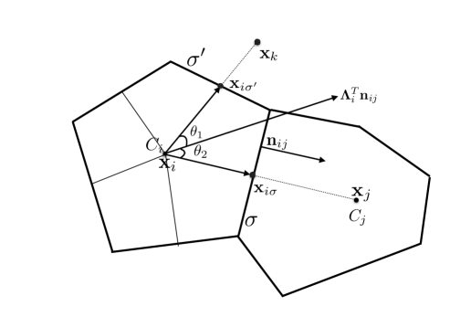
Figure 1: A sketch illustrating the calculation of the one-sided anisotropic heat flux across the face $\sigma$, which is shared by the two Voronoi cells $C_{i}$ and $C_{j}$. ${\bf n}_{ij}$ is the unit vector perpendicular to $\sigma$, ${\bf x}_{i}$, ${\bf x}_{j}$ and ${\bf x}_{k}$ are the centers of cells $C_{i}$, $C_{j}$ and $C_{k}$, respectively, $\theta_{1}$ is the angle between ${\bf x}_{i\sigma}$ and ${\bf\Lambda}_{i}^{T}{\bf n}_{ij}$, $\theta_{2}$ is the angle between ${\bf x}_{i\sigma^{\prime}}$ and ${\bf\Lambda}_{i}^{T}{\bf n}_{ij}$, and ${\bf x}_{i\sigma}$ and ${\bf x}_{i\sigma^{\prime}}$ are the harmonic averaging points defined by Eqn. (20).

We can also rewrite Equation (10) as

$${\bf j}=-\frac{\kappa}{c_{v}}[{\bf b}({\bf b}\cdot{\bf\nabla}u)],$$ (11)

by replacing temperature for an ideal gas with the internal energy per unit mass

$$u=\frac{k_{B}T}{(\gamma-1)\mu}=c_{v}T,$$ (12)

where $\gamma$ is the adiabatic index, and $\mu$ is the mean molecular weight. The value of $\mu$ depends on the temperature, ionization state and the composition of the gas. Since we are dealing mainly with a high temperature, low metallicity plasma of primordial composition we assume that the gas is fully ionised and consequently set the mean molecular weight to the constant value $\mu\sim 0.6\,m_{p}$. The final equation for anisotropic thermal conduction then becomes

$$\frac{\partial u}{\partial t}=\frac{1}{c_{v}\rho}{\bf\nabla}\cdot[\kappa{\bf b}({\bf b}\cdot{\bf\nabla})u],$$ (13)

and below we focus on studying numerical solutions schemes for this partial differential equation.

3 Methods

This section describes the spatial discretisation and time integration techniques we employ to solve Eqn. (13).

3.1 Spatial discretisation

Consider first the spatial part of Eqn. (13), which takes the form of a linear operator of the form

$$\mathcal{L}u=\frac{1}{c_{v}\rho}{\bf\nabla}\cdot[\kappa{\bf b}({\bf b}\cdot{\bf\nabla})u].$$ (14)

Since Arepo is a finite volume code which divides the computational domain into a set of control volumes, the above equation can be recast into the form

$$\mathcal{L}u=\lim_{V\to 0}\frac{1}{V}\int_{V}\frac{1}{c_{v}\rho}{\bf\nabla}\cdot[\kappa{\bf b}({\bf b}\cdot{\bf\nabla})u]\,{\rm d}V,$$ (15)

and by applying Gauss’ divergence theorem we get

$$\begin{split}\mathcal{L}u&=\lim_{V\to 0}\frac{1}{V}\int_{\partial V}\frac{1}{c_{v}\rho}[\kappa{\bf b}({\bf b}\cdot{\bf\nabla})u]\cdot{\bf n}\,{\rm d}A.\end{split}$$ (16)

Therefore, the approximated heat flux in a finite-volume scheme for each cell $i$ with $N_{i}$ neighbours is

$$\begin{split}\mathcal{L}u_{i}&=\sum_{j=i}^{N_{i}}{\bf\Lambda}_{i}({\bf\nabla}u)_{i}\cdot{\bf n}_{ij}({\rm d}A)_{ij}\\ &=\sum_{j=i}^{N_{i}}({\bf\nabla}u)_{i}\cdot{\bf\Lambda}_{i}^{T}{\bf n}_{ij}({\rm d}A)_{ij},\end{split}$$ (17)

where

$${\bf\Lambda}_{i}=\frac{\kappa_{i}}{c_{v}m_{i}}\begin{cases}\hfill{\bf b}_{i}\otimes{\bf b}_{i}\hfill&\rm{snisotropic\ conduction},\\ \hfill\mathds{1}\hfill&\rm{isotropic\ conduction},\\ \end{cases}$$ (18)

and ${\bf n}_{ij}$ is the unit vector perpendicular to the face of area $({\rm d}A)_{ij}$ shared between cells $C_{i}$ and $C_{j}$.

We employ the method described in GW13 for splitting the one-sided facet heat fluxes into normal and oblique components, followed by a limiting of the oblique fluxes. In 2D, the flux splitting is achieved by decomposing ${\bf\Lambda}_{i}^{T}{\bf n}_{ij}$ in terms of two vectors, as sketched in Fig. 1:

$$\begin{split}{\bf\Lambda}_{i}^{T}{\bf n}_{ij}&=\zeta_{i\sigma}({\bf x}_{i\sigma}-{\bf x}_{i})+\zeta_{i\sigma^{\prime}}({\bf x}_{i\sigma^{\prime}}-{\bf x}_{i}),\\ \zeta_{i\sigma}&=\frac{||{\bf\Lambda}_{i}^{T}{\bf n}_{ij}||\sin\theta_{2}}{||{\bf x}_{i\sigma}-{\bf x}_{i}||\sin(\theta_{2}+\theta_{1})},\\ \zeta_{i\sigma^{\prime}}&=\frac{||{\bf\Lambda}_{i}^{T}{\bf n}_{ij}||\sin\theta_{1}}{||{\bf x}_{i\sigma^{\prime}}-{\bf x}_{i}||\sin(\theta_{2}+\theta_{1})},\\ \end{split}$$ (19)

where ${\bf x}_{i}$ and ${\bf x}_{j}$ are the centers of cells $C_{i}$ and $C_{j}$, $\theta_{1}$ is the angle between ${\bf x}_{i\sigma}$ and ${\bf\Lambda}_{i}^{T}{\bf n}_{ij}$, $\theta_{2}$ is the angle between ${\bf x}_{i\sigma^{\prime}}$ and ${\bf\Lambda}_{i}^{T}{\bf n}_{ij}$, and the point ${\bf x}_{i\sigma}$ is the harmonic averaging point defined as (similar definition applies for ${\bf x}_{i\sigma^{\prime}}$),

$$\begin{split}{\bf x}_{i\sigma}({\sigma\in C_{i}\cap C_{j}})=\frac{d_{j\sigma}\lambda_{ij}{\bf x}_{i}+d_{i\sigma}\lambda_{ji}{\bf x}_{j}}{d_{j\sigma}\lambda_{ij}+d_{i\sigma}\lambda_{ji}}.\end{split}$$ (20)

Here, $d_{i\sigma}$ is the orthogonal distance from the center of the cell $C_{i}$ to face $\sigma$, and $\lambda_{ij}={\bf n}^{T}_{ij}{\bf\Lambda}_{i}{\bf n}_{ij}$.

For a given set of points, a Voronoi tessellation of space consists of non-overlapping cells around each of the cell generating points such that each cell contains the region of space closer to it than any of the other points. A consequence of this definition is that the cells are polygons in 2D and polyhedra in 3D, with faces that are equidistant to the mesh-generating points of each pair of neighboring cells i.e., $d_{i\sigma}=d_{j\sigma}=d_{ij}/2$. Therefore, Eqn. (20) can be rewritten as

$${\bf x}_{i\sigma}=\omega_{ij}{\bf x}_{i}+\omega_{ji}{\bf x}_{j},$$ (21)

where

$$\omega_{ij}=\frac{\lambda_{ij}}{\lambda_{ij}+\lambda_{ji}},$$ (22)

with $\omega_{ji}=1-\omega_{ij}$, and correspondingly, the internal energy at these points is interpolated as

$$\begin{split}u({{\bf x}_{i\sigma}})=u_{\sigma}=\omega_{ij}u_{i}+\omega_{ji}u_{j}.\end{split}$$ (23)

Similarly, in 3D, three non-coplanar vectors are needed to express the anisotropic diffusion vector

$$\begin{split}{\bf\Lambda}_{i}^{T}{\bf n}_{ij}&=\zeta_{i\sigma}({\bf x}_{i\sigma}-{\bf x}_{i})+\zeta_{i\sigma^{\prime}}({\bf x}_{i\sigma^{\prime}}-{\bf x}_{i})+\zeta_{i\sigma^{\prime\prime}}({\bf x}_{i\sigma^{\prime\prime}}-{\bf x}_{i}).\end{split}$$ (24)

Hence, we can in general write down ${\bf\Lambda}_{i}^{T}{\bf n}_{ij}$ as

$$\begin{split}{\bf\Lambda}_{i}^{T}{\bf n}_{ij}&=\sum_{\sigma_{n},n=1}^{N_{\rm dims}}\zeta_{i\sigma_{n}}({\bf x}_{i\sigma_{n}}-{\bf x}_{i}).\\ \end{split}$$ (25)

Substituting Eqn. (25) back into Eqn. (17), the one-sided flux across the face $\sigma$ from $C_{i}$ to $C_{j}$ is written as,

$$\begin{split}F_{ij}&=|\sigma|{\bf\nabla}u\cdot\sum_{\sigma_{n}}\zeta_{i\sigma_{n}}({\bf x}_{i\sigma_{n}}-{\bf x}_{i}),\\ &=|\sigma|\sum_{\sigma_{n}}\zeta_{i\sigma_{n}}(u_{i\sigma_{n}}-u_{i}).\end{split}$$ (26)

Now we have a way of decomposing this flux into normal ($F^{(1)}$) and oblique ($F^{(2)}$) components,

$$\begin{split}F_{ij}&=F^{(1)}_{ij}+F^{(2)}_{ij},\\ F^{(1)}_{ij}&=a_{\sigma\sigma}^{i}(u_{i\sigma}-u_{i}),\\ F^{(2)}_{ij}&=\sum_{\sigma^{\prime}\neq\sigma}a_{\sigma\sigma^{\prime}}^{i}(u_{i\sigma^{\prime}}-u_{i}),\end{split}$$ (27)

where $a_{\sigma\sigma^{\prime}}^{i}=|\sigma|\zeta_{i\sigma^{\prime}}$. To make it locally conservative ($F_{ij}=-F_{ji}$), we rework the net flux in the following form:

$$\begin{split}F_{ij}^{\rm{net}}&=\mu_{ij}F^{(1)}_{ij}-\mu_{ji}F^{(1)}_{ji}+\mu^{p}_{ij}\left[1-{\rm sign}(F^{(2)}_{ij}F^{(2)}_{ji})\right]F^{(2)}_{ij},\\ \rm{where}\ &\mu_{ij}=\frac{|F^{(2)}_{ji}|+\epsilon}{|F^{(2)}_{ij}|+|F^{(2)}_{ji}|+2\epsilon},\\ \rm{and}\ &\mu^{p}_{ij}=\frac{|F^{(2)}_{ji}|}{|F^{(2)}_{ij}|+|F^{(2)}_{ji}|+2\epsilon}.\end{split}$$ (28)

Notice that the oblique flux component depends on the current estimates of the two one-sided oblique fluxes.

The salient point is that GW13 prove that this form of the flux is locally conservative and obeys the DEP under the condition that $\zeta_{i\sigma}>0\ \forall\ [i,\sigma]$ ($\zeta_{i\sigma}$ is defined by Eqn. 19). This condition is automatically satisfied for a Voronoi mesh as it is convex by construction (see GW13 for more details). A convex polygon is defined as a polygon with all internal angles less than $180^{\circ}$. This property implies that no matter the orientation of ${\bf\Lambda}_{i}^{T}{\bf n}_{ij}$, there always exist ${\bf x}_{i\sigma}$’s such that all $\zeta_{i\sigma}$’s are positive.

The most computationally intensive part of this calculation is the estimation of the $\zeta_{i,\sigma}$. In essence, this involves determining the triangle within which ${\bf\Lambda}_{i}^{T}{\bf n}_{ij}$ lies in 2D, while in 3D it reduces to determining the tetrahedron which encompasses this vector. Unfortunately, if a cell $C_{i}$ has $N_{i}$ neighbours, a naive implementation of this operation has a complexity of $\mathcal{O}(N_{i}^{3})$ in 3D, which is highly undesirable. Instead we make use of the fact that Arepo first creates a Delaunay tessellation and then obtains the Voronoi tessellation from it. The Delaunay tessellation is formed by triangles/tetrahedra that do not contain any of the points inside their circumspheres (see Springel 2010 for more details). Therefore, in order to compute the $\zeta_{i,\sigma}$, we just determine in which of the Delaunay triangles/tetrahedra connected to the cell $C_{i}$ the vector ${\bf\Lambda}_{i}^{T}{\bf n}_{ij}$ lies. This reduces the complexity of the algorithm to $\mathcal{O}(N_{\rm tetra})$, where $N_{\rm tetra}$ are all the points which have a Delaunay connection to $C_{i}$ (these can also be points where the area of the face between the points is zero).

In passing we note that the dynamic movement of the mesh in Arepo does not affect our basic implementation. Mesh motion is completely taken care of by the hydro solver; the diffusion solver only sees a static mesh since we couple it to the rest of the dynamics through operator splitting.

3.2 Time integration

The simplest way to perform the time integration is to do it explicitly. However, numerical stability requires that the timestep is limited by the von Neumann stability condition $\Delta t\leq\eta_{N}(\Delta x)^{2}/\chi$ where $\Delta x$ is the cell width, $\chi=\kappa/(c_{v}\rho)$ and $\eta_{N}<1$ is the von Neumann stability coefficient which we usually set to $0.2$. This timestep constraint becomes rather severe, especially at high resolution (given its quadratic dependence on $\Delta x$) and in high temperature plasmas. Therefore, an implicit method that places no stability limit on the diffusion timestep is highly desirable.

The easiest implicit time discretisation is the first order backwards Euler method,

$$\frac{u_{i}^{t+\Delta t}-u_{i}^{t}}{\Delta t}=\sum_{j=i}^{N_{i}}A_{ij}(u_{j}^{t+\Delta t}-u_{i}^{t+\Delta t}),$$ (29)

where $A_{ij}$ is the coefficient matrix defined as

$$F_{i}=\sum_{j}A_{ij}(u)(u_{j}-u_{i}).$$ (30)

$A_{ij}$ can be split into normal ($\alpha_{ij}$) and oblique ($\beta_{ij}$) components,

$$\begin{split}A_{ij}&=\alpha_{ij}+\beta_{ij}(u),\\ \end{split}$$ (31)

which in turn are defined as

$$\begin{split}\alpha_{ij}&=\mu_{ij}a_{\sigma\sigma}^{i}\omega_{ji}+\mu_{ji}a_{\sigma\sigma}^{j}\omega_{ij},\\ \beta_{ij}(u)&=\omega_{ji}\sum_{k,\sigma^{\prime}\in C_{i}\cap C_{k}}\mu_{ik}^{p}\ [1-{\rm sign}(F^{(2)}_{ik}(u)F^{(2)}_{ki}(u))]\ a_{\sigma^{\prime}\sigma}^{i}.\end{split}$$ (32)

Equation (29) can be rewritten as

$$\begin{split}u_{i}^{t+\Delta t}-\Delta t\sum_{j=i}^{N_{i}}A_{ij}(u_{j}^{t+\Delta t}-u_{i}^{t+\Delta t})=u_{i}^{t}.\end{split}$$ (33)

Focussing on the left-hand-side of this equation, we obtain

$$\begin{split}&{\rm L.H.S}=u_{i}^{t+\Delta t}+\Delta t\sum_{k=i}^{N_{i}}A_{ik}u_{i}^{t+\Delta t}-\Delta t\sum_{j=i}^{N_{i}}A_{ij}u_{j}^{t+\Delta t}\\ &=\sum_{j=i}^{N_{i}}\left(\delta_{ij}u_{j}^{t+\Delta t}+\Delta t\sum_{k=i}^{N_{i}}A_{ik}\delta_{ik}u_{k}^{t+\Delta t}\right)-\Delta t\sum_{j=i}^{N_{i}}A_{ij}u_{j}^{t+\Delta t}.\\ \end{split}$$ (34)

Therefore the equation we have to solve is given by

$$\begin{split}\sum_{j=i}^{N_{i}}\left(\delta_{ij}\left(1+\Delta t\sum_{k=i}^{N_{i}}A_{ik}\right)-\Delta tA_{ij}\right)u_{j}^{t+\Delta t}=u_{i}^{t},\\ \end{split}$$ (35)

which is of the generic form

$${\bf A}({\bf U})\,{\bf U}={\bf U}_{0},$$ (36)

where ${\bf U}_{0}=\{u_{i}^{t}\}$ is the internal energy vector at the present time. The dependence of the coefficient matrix ${\bf A}$ on the internal energy vector makes the the system non-linear.

This nonlinear system can be solved by Picard’s iterative method (Dembo et al., 1982). This approach linearizes the non-linear system by estimating the value of the coefficient matrix from the values of the internal energy obtained from the previous iteration. The algorithm to solve the full non-linear system is then given by

1. Solve the linear system ${\bf A}({\bf U}^{n-1}){\bf U}_{*}^{n}={\bf U}_{0}$ with respect to ${\bf U}_{*}^{n}$.

2. Relax the solution ${\bf U}^{n}=\mu^{n}{\bf U}_{*}^{n}+(1-\mu^{n}){\bf U}^{n-1}$, where $\mu^{n}$ is relaxation parameter given by Eqn. (38).

3. Break if $\frac{||{\bf A}({\bf U}^{n}){\bf U}^{n}-{\bf U}_{0}||}{||{\bf A}({\bf U}_{0}){\bf U}_{0}-{\bf U}_{0}||}<10^{-3}$ or $\frac{||{\bf U}^{n}-{\bf U}^{n-1}||}{||{\bf U}_{0}||}<10^{-6}$.

4. Else set ${\bf U}^{n-1}={\bf U}^{n}$, and repeat.

We use the hypre library to solve the linear system in step (i). hypre is a library for solving large, sparse linear systems of equations on massively parallel computers (Falgout & Yang, 2002). In particular, the linear system is solved using the generalised minimal residual (GMRES) iterative method (Saad & Schultz, 1986). Additionally an algebraic multi-grid preconditioner (Henson & Yang, 2002) is used in order to achieve faster convergence. The tolerance limit for iteratively solving the linear system is set to $\epsilon_{\rm lin}=10^{-8}$.

A Picard iteration consists of solving ${\bf A}({\bf U}_{-}){\bf U}={\bf B}$ until convergence. This has several drawbacks in practice. If successive correction vectors, ${\bf C}^{n-1}={\bf U}^{n}-{\bf U}^{n-1}$ and ${\bf C}^{n}={\bf U}^{n+1}-{\bf U}^{n}$, are in roughly the same direction, the scheme is undershooting. This means ${\bf C}^{n-1}$ could have been larger, reducing the number of iterations. This can in principle be improved by overrelaxation, i.e. taking instead of ${\bf U}^{n}$ a larger step $\mu{\bf U}^{n}$ with $\mu>1$. On the other hand, if ${\bf C}^{n}$ is roughly in the opposite direction to ${\bf C}^{n-1}$, the scheme is overshooting the solution. In the worst case, this can lead to an endless sequence of correction vectors oscillating around the actual solution. Overshooting can be remedied by underrelaxation, i.e. taking a smaller step $\mu{\bf U}^{n}$ with $0<\mu<1$.

We use a variant of the unstable manifold corrector scheme outlined in (De Smedt et al., 2010) to adaptively under- or overrelax the solution (as in step (iii) of the non-linear implicit algorithm). Let us define the angle ($\theta$) between the correction vectors as

$$\theta^{n}={\rm cos}^{-1}\left(\frac{({\bf C}_{*}^{n-1})^{T}\cdot{\bf C}^{n-2}}{||{\bf C}_{*}^{n-1}||\cdot||{\bf C}^{n-2}||}\right),$$ (37)

and then over- or underrelax the solution according to the value of $\theta$,

$$\mu^{n}=\begin{cases}\hfill 1.5\hfill&\theta^{n}\leq\frac{\pi}{8}\\ \hfill 1.0\hfill&\frac{\pi}{8}<\theta^{n}\leq\frac{3\pi}{4}\\ \hfill 0.5\hfill&\frac{3\pi}{4}<\theta^{n}\leq\frac{9\pi}{10}\\ \hfill 0.3\hfill&\theta^{n}>\frac{9\pi}{10}.\\ \end{cases}$$ (38)

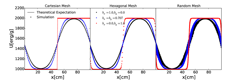
Figure 2: Diffusion of a temperature step function in the presence of a magnetic field in the direction of the temperature gradient (black curves), inclined by $45^{\circ}$ (blue curves) relative to the temperature gradient, and perpendicular to the temperature gradient (red curves) at $t=5\,{\rm s}$. The test is performed for three different configurations of the mesh, regular Cartesian (left panel), regular hexagonal (middle panel) and a random mesh (right panel). The resolution is $100^{2}$ particles within the domain. The points are the simulations results and the solid curves are the theoretical expectations.

This fully implicit scheme is unconditionally stable. However, it is also computationally expensive because we need to perform non-linear iterations on top of the linear iterations at each step. In our test problems, presented in Section 4, an average of 10-15 nonlinear iterations were required per timestep. This reflects the fact that in order to achieve a significant speedup in the calculation, one needs to set $\eta_{N}\geq 100$. Therefore, this method is only viable if the magnetic fields are slowly varying, over characteristic timescales of order $\sim 100$ times the conduction timescale.

Therefore, for problems where the accuracy over a short period of the magnetic field is important (for example see Section 4.5) we implement a semi-implicit algorithm following the method outlined in Sharma & Hammett (2011). Here the terms of the coefficient matrix that depend on the internal energy are integrated explicitly, while the other terms are integrated implicitly. Accordingly, Eqn. (35) changes form and becomes

$$\begin{split}\sum_{j=i}^{N_{i}}\left(\delta_{ij}\left(1+\Delta t\sum_{k=i}^{N_{i}}\alpha_{ik}\right)-\Delta t\alpha_{ij}\right)u_{j}^{t+\Delta t}=\\ u_{i}^{t}+\Delta t\sum_{l=1}^{N_{i}}F^{(2)}_{il}(u_{l}^{t},u_{i}^{t}).\\ \end{split}$$ (39)

In this form, the coefficient matrix is independent of the current value of the internal energy, and therefore the system is linear. As with the fully implicit scheme, this linear system is solved using the hypre library with the GMRES routine and a multigrid preconditioner. We numerically verify that this method is stable up to $\eta_{N}=4$, which is still an improvement by a factor of $\sim 10-20$ over the explicit scheme. As mentioned in Sharma & Hammett (2011), the explicit treatment of the oblique flux terms means that this scheme is not strictly obeying the DEP, but the deviations from it are very small and the corresponding oscillations are damped with time. This method is extremely fast as it requires only the solution of a linear system per timestep.

One drawback of the implicit schemes is that it is not directly compatible with the individual time-stepping method used in Arepo for advancing ordinary hydrodynamics. We presently overcome this by solving the conduction equation only on global synchronization timesteps of the code. This is a viable approach because the fully implicit scheme is unconditionally stable and does not pose strong constraints on the permissible timestep. However, the timestep restriction of the semi-implicit method implies that when this method is used we need to restrict the global timestep in the simulation to $\eta_{N}$ times the minimum of the diffusion step size of all cells in the domain

4 Numerical Tests

In this section we present the results from various numerical tests of our anisotropic conduction implementation. The relevant hydrodynamics equations are evolved using the moving mesh finite volume scheme outlined in Springel (2010), with the improved time integration and gradient estimation techniques described in Pakmor et al. (2016). The magnetic fields which decide the direction of diffusion are evolved using the ideal MHD module outlined in Pakmor & Springel (2013) based on the 8-wave formalism to control divergence errors (Powell et al., 1999).

Sections 4.1, 4.2 and 4.3 are intended to test the accuracy and the stability of the anisotropic conduction implementation only, without evolving the hydrodynamical equations. Therefore, in all these tests, the cells do not move and only interact with each other through heat conduction (i.e. the gas dynamics is not explicitly followed and the gas velocity is fixed to zero at all times). This also ensures that the magnetic fields are constant with time.

In Sections 4.4 and 4.5, we additionally test the accuracy of the anisotropic conduction scheme when hydrodynamics and heat conduction are coupled. In these tests, we initially start with a regular Cartesian grid, which is then allowed to move and distort according to the local fluid motion (Springel, 2010). In addition, the mesh is regularized where needed using the scheme outlined in Vogelsberger et al. (2012). The time integration in all these tests is performed with the semi-implicit scheme outlined in Section 3.2, using $\eta_{N}=4$.

4.1 Diffusion of a step function

As a first test of our implementation, we study the diffusion of a temperature step function. We perform 2D simulations with a domain size of $(100\,{\rm cm})^{2}$ sampled with $(100)^{2}$ cells. The internal energy (in erg/g) of a given cell is set to

$$u(x,y)=\begin{cases}\hfill 1000\hfill&x\leq 50\\ \hfill 2000\hfill&x>50.\end{cases}$$ (40)

The density is kept constant at $\rho=1\,\rm{g\,cm^{-3}}$ throughout the computational domain. We set the diffusivity to be

$$\chi=\frac{\kappa}{c_{v}\rho}=10\ \rm{cm^{2}\,s^{-1}},$$ (41)

and adopt periodic boundary conditions at the domain edges. The analytic solution for this problem under periodic boundary conditions is given by

$$\begin{split}U(x,t)&=u_{0}+\frac{\Delta u}{2}\sum_{x_{i},i=1}^{3}\left[(-1)^{i}{\rm erf}\left(\frac{x-x_{i}}{\sqrt{4\chi tb_{x}^{2}}}\right)\right],\end{split}$$ (42)

with $x_{1}=0$, $x_{2}=50$, $x_{3}=100$, $u_{0}=1500$ and $\Delta u=1000$.

We perform this test with three different kinds of meshes, Cartesian, hexagonal and random. The random mesh is created by choosing points inside the simulation domain whose coordinates are a pair of random deviates extracted from a uniform probability distribution in the interval bounded by the domain and letting Arepo construct a Voronoi mesh out of these random points. Fig. 2 shows the results of the temperature step function test on the three different meshes at time $t=5\,s$. The red points show the internal energy evolution when the magnetic field is perpendicular to the temperature gradient (${\bf b}=\{0,1\}$), blue points when the magnetic field and the temperature gradient are are misaligned by $\pi/4$ (${\bf b}=1/\sqrt{2}\{1,1\}$) and the black points when the magnetic field direction and the temperature gradient is aligned (${\bf b}=\{1,0\}$). The left panel shows the result for the Cartesian mesh, the middle panel for the hexagonal mesh and the right panel for the random mesh.

It is evident that the simulation results agree well with the analytic solution (solid curves). We have also verified that our implementation obeys the DEP in this test. Even when the magnetic field is perpendicular to the direction of the temperature gradient, the algorithm performs remarkably well and does not give rise to unstable oscillations. Arth et al. (2014), for example, had to add an isotropic component to their anisotropic diffusion tensor in order to stop unphysical oscillations. While we do have some amount of perpendicular numerical diffusion, this appears to be very small, something we will further quantify in Section 4.3.

Another point to notice is that although the random mesh simulations do well on average, i.e., the mean temperature of the cell at the particular value of $x$ matches the analytical expectation well, there is some amount of scatter around the mean. We argue that this scatter does not arise because of an incorrect calculation of the heat fluxes on a random mesh, but because the boundaries of the random mesh are not regularly spaced in $x$ (i.e. along the direction of the temperature gradient). The difference in sizes of the cells in a random mesh makes the conduction front irregular, giving rise to the observed temperature scatter.

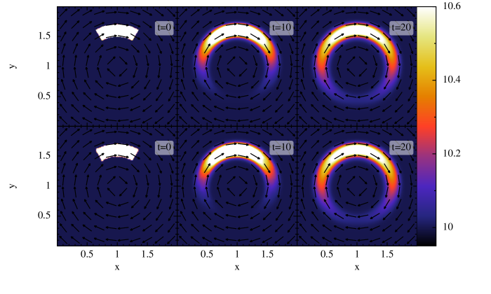
Figure 3: Time evolution of a hot patch of gas under a circular magnetic field in 2D. The test is performed for both a regular Cartesian (top panel) and a random mesh (bottom panel). The resolution is $400^{2}$ particles within the domain. The arrows represent the orientation of the magnetic field and the colour bar shows the internal energy of the gas in ${\rm erg\,g^{-1}}$. This plot was created using the interactive visualization tool Splash (Price, 2007).

4.2 Diffusion of a hot patch of gas in a circular magnetic field

We investigate the circular diffusion problem as outlined in Parrish & Stone (2005) and Sharma & Hammett (2007). A hot patch of gas surrounded by a cooler background is allowed to diffuse in the presence of a circular magnetic field. The temperature drops discontinuously across the patch boundary. The computational domain is of size ($2\ \rm{cm}$)² with periodic boundary conditions.

We perform this test for a regular Cartesian grid and a random mesh (as in Section 4.1). The regular Cartesian mesh describes the behaviour of the code in the best case scenario where the regularity of the mesh inherently reduces the errors, whereas the random mesh corresponds to the worst case scenario where in certain situations the mesh can be stretched and distorted by large amounts due to fluid motion. The behaviour of the mesh and hence the degree of mesh related errors can be controlled by regularizing the mesh, using schemes such as the ones described in Springel (2010), Vogelsberger et al. (2012) and Mocz et al. (2015).

The initial internal energy (in $\rm{erg/g}$) distribution is given by

$$u(x,y)=\begin{cases}\hfill 12\hfill&\mbox{for}\ 0.5<r<0.7\ \rm{and}\ abs(\theta)<\pi/6,\\ \hfill 10\hfill\ &\rm{otherwise},\end{cases}$$ (43)

where $r=\sqrt{(x-1)^{2}+(y-1)^{2}}$ and $\theta=\tan^{-1}[(y-1)/(x-1)]$. The magnetic fields are circular and centered on [1,1]. The density is set to unity. The diffusivity $\chi$ is set to $0.01\ \rm{cm^{2}\,s^{-1}}$. The simulation is run until time $t=200\,{\rm s}$. There is no explicit perpendicular diffusion coefficient, so ideally the internal energy outside the ring ($r\leq 0.5$ and $r\geq 0.7$) stays always $10$. The initial hot gas should only diffuse along the azimuthal magnetic field until at the end it is evenly distributed in a ring.

We note that in the coordinate defined as $s=r\theta$, the problem reduces to the diffusion of a double step function. This is valid while no material has diffused more than halfway across the ring. Therefore, the analytic solution is of the same form as Eqn. 42 in the co-ordinate $s$ with $b_{x}=1$. Fig. 3 shows the internal energy distribution at times $t=0\,{\rm s}$ (left panels), $t=10\,{\rm s}$ (middle panels) and $t=20\,{\rm s}$ (right panels) for both a Cartesian (top panels) and random (bottom panels) grid simulations. The evolution of the internal energy is quite similar and is independent of the mesh used. We further quantify this by looking at the L1 error in the simulations. Figure 4 plots the L1 error at $t=10\,{\rm s}$ in the simulation as a function of the resolution for both Cartesian (solid curve) and random (dot-dashed curve) meshes.

The convergence order for the Cartesian mesh is about $0.49$ and for the random mesh about $0.41$. This convergence order is smaller than the limited symmetric method, but similar to the values obtained by other slope limited schemes (Sharma & Hammett, 2007). A better interpolation scheme and a better non-linear flux limiter that is both conservative and DEP-preserving can potentially improve the convergence order of our scheme. However, it is quite a challenge to achieve this, especially for unstructured meshes.

Perpendicular diffusion is an unwanted side effect of the non-linear flux limited scheme. Although the limited fluxes are more diffusive, we numerically verify that they never undershoot below the minimum or overshoot above the maximum temperature. The limiter hence ensures the stability of the scheme but reduces the accuracy.

4.3 Sovinec test

The limiting of the oblique fluxes results in higher perpendicular numerical diffusion. It is quite important to quantify this artificial numerical diffusivity in order to understand the limitations of our implementation. We estimate the numerical diffusivity by performing the experiment suggested in Sovinec et al. (2004). We perform this test for both Cartesian and random meshes (as in Section 4.1) in 2D.

Let us consider the full heat conduction equation (i.e. a generalization of Eqn. 13),

$$\frac{\partial u}{\partial t}={\bf\nabla}\cdot[\kappa_{||}{\bf b}({\bf b}\cdot{\bf\nabla})u]+{\bf\nabla}\cdot[(\kappa_{\perp}+\kappa_{\rm num})(\mathds{1}-({\bf b}\otimes{\bf b})){\bf\nabla}u]+Q.$$ (44)

where $Q$ is a source function of the form $Q=Q_{0}\cos(kx)\cos(ky)$, and we set $\rho c_{v}=1$. We further assume a fixed magnetic field such that ${\bf B}\cdot{\bf\nabla}u=0$ and also set $\kappa_{\perp}=0$. We use non-periodic boundary conditions with the temperature at the boundary fixed to $T_{\rm bound}=0$, which means that the boundaries act as a heat sink. Then the steady state solution of Eqn. (44) at the center of the domain is $u(0,0)=Q_{o}/(2k^{2}\kappa_{\rm num})$. Therefore the perpendicular numerical diffusivity can be easily deduced from the value of the central internal energy.

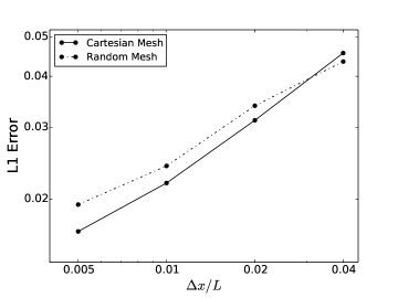
Figure 4: L1 error, at $t=10\,{\rm s}$, as a function of resolution for a Cartesian (solid line) and a random mesh (dot dashed line) for simulations of the diffusion of a hot patch of gas in circular magnetic fields (Section 4.2). The convergence order for the Cartesian mesh is $0.49$, and $0.41$ for the random meshes.

We simulate this configuration in a domain of size $[-0.5,0.5]\times[-0,5,0.5]$ with density $\rho=1$, $k=\pi$ and $Q_{0}=2\pi^{2}$. The initial temperature is $T(x,y)=\cos(\pi x)\cos(\pi y)$ and the magnetic field components are set to $B_{x}=\cos(\pi x)\sin(\pi y)$ and $B_{y}=-\sin(\pi x)\cos(\pi y)$, so that the value of the numerical perpendicular diffusivity can be estimated from $\kappa_{\rm num}=1/u(0,0)$ once the system reaches the steady state. We then measure the ratio $\kappa_{||}/\kappa_{\rm num}$ as a function of resolution and plot the results is Fig. 5. We see that even at really low resolution the value of the perpendicular numerical diffusivity is just about $3\%$ the value of $\kappa_{||}$. This is comparable to the numerical diffusivity obtained from slope limited methods such as in Sharma & Hammett (2007). We also note that the convergence order in Cartesian meshes is about $-1.63$, again in agreement with previous methods. The convergence order for random meshes is about $-1.31$, which is lower than the one determined for Cartesian meshes. This is mainly caused by the different cell sizes (and therefore different local resolutions) in different parts of the domain.

4.4 Point explosion with heat conduction

We next test our conduction implementation for the Sedov-Taylor blast wave problem. This problem is a good test to determine the accuracy of coupling two distinct physical processes: hydrodynamics and diffusion. We simulate three different configurations of the blast wave problem, the classical adiabatic blast wave test, the blast wave test with isotropic conduction, and the blast wave test with anisotropic conduction in 3D. We simulate a domain of size $100$ pc on a side with $64^{3}$ resolution elements to begin with.

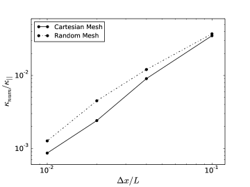
Figure 5: Relative numerical perpendicular diffusion coefficient as a function of resolution as obtained from the Sovinec test (Section 4.3). The convergence order is about $1.63$ for Cartesian meshes (solid line) and $1.31$ for random meshes (dot-dashed line).

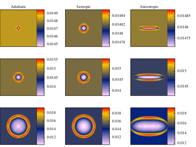
Figure 6: Projected gas density maps in the $xy$-plane of an adiabatic point explosion (left column), and point explosions with isotropic (middle column) and anisotropic (right column) conduction at 1 (top row), 10 (middle row) and 100 (bottom row) kyrs. The magnetic field strength is $1{\rm\mu G}$, pointing in the positive $x$-direction. The size of each panel is (100 pc)². The resolution is $64^{3}$ particles within the domain. This plot was created using the interactive visualization tool Splash.

We inject $E_{0}=3.33\times 10^{50}\ \rm{erg}$ of energy into the central 8 cells. The blast wave expands into a uniform medium of density $\rho_{0}=1\ \rm{cm}^{-3}$ and temperature $T=10^{4}\ {\rm K}$. A uniform magnetic field pointing in the positive $x$-direction of strength $1\,{\rm\mu G}$ is added to each gas cell. This low value of the magnetic field ensures that it is not important for the dynamics of the explosion. We hence expect the blast wave to expand spherically without any hindrance from the magnetic field. All three simulations are performed for a total of $10^{5}$ yr. The adiabatic index is set to $\gamma=5/3$. For this test problem, we do not include the effect of saturation when calculating the conduction heat flux and we set the value of the conduction coefficient $\kappa$ to the full Spitzer value (Eqn. 6).

Fig. 6 shows the resulting density maps of the adiabatic (left column), isotropic conduction (middle column) and anisotropic conduction (right column) simulations at 1 (top row), 10 (middle row) and 100 (bottom row) kyrs. We can see right away that the results are very different. Qualitatively, the conduction front outpaces the shock front during the initial phase of expansion ($<10$ kyrs) in the isotropic conduction simulation, while anisotropic conduction seems to accelerate the shock in the direction of the magnetic field while the shock front in the perpendicular direction lags behind. At late times (100 kyrs), the shock front in the isotropic and the adiabatic cases appears to be in the same position. The perpendicular shock front in the anisotropic conduction simulation still lags behind.

Figures 7 and 8 show the results in a more quantitative manner at two different times, $3$ kyr and $80$ kyr, respectively. The solid black lines correspond to the classical adiabatic solutions for the pressure, density and temperature structure in the shock. As we can see clearly, the adiabatic simulation (left column) accurately traces the theoretical expectations (Sedov, 1959) for the pressure (top row), density (middle row) and temperature (bottom) structure behind the shock. In the following subsections, we describe in more detail the structure of the solution when isotropic and anisotropic thermal conduction are included in the calculations.

4.4.1 Point explosion with isotropic heat conduction

The evolution of the point explosion with heat conduction was considered in detail by Reinicke & Meyer-Ter-Vehn (1991). They obtain self-similar solutions under the assumption that the ambient gas density decays with a given power of the radius. However, if the density is constant, then the solution is no longer self-similar. However, the solution can be obtained by analysing the corresponding pure hydrodynamics and pure diffusion problems, each of which has a similarity solution.

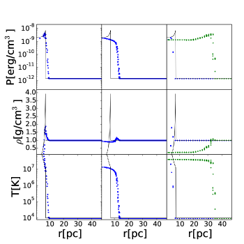
Figure 7: Pressure (top row), density (middle row) and temperature (bottom row) profiles in the point explosion with adiabatic (left column), isotropic (middle column) and anisotropic conduction (right column) at $t=3$ kyr. The solid lines plot the analytic solution of the classical adiabatic Sedov-Taylor problem. The blue points are the simulation results. For anisotropic conduction, we plot two profiles, one along the magnetic field direction (green points) and the other perpendicular to it (blue points).

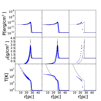
Figure 8: Same as Fig. 7 but for $t=80\,{\rm kyr}$. The anisotropic conduction plots do not have any green simulation points because the shock front in the direction of the magnetic field has progressed beyond the computational domain.

The position $r_{a}$ of the shock front in the pure adiabatic Sedov solution is given by

$$r_{a}=\beta_{a}(E_{0}t^{2}/\rho_{0})^{1/5},$$ (45)

where $\beta_{a}\sim 1.15$, $E_{0}$ is the energy input and $\rho_{0}$ is the background density of the medium. For the isotropic conduction problem (middle column of Fig. 7 and 8), let us consider a diffusivity of the form $\chi=\chi_{0}\rho^{a}T^{b}$. In our case, $a=0$ and $b=5/2$. For these parameters, the position $r_{c}$ of the conduction front is given by (Zeldovich & Raizer, 1966; Barenblatt & Cole, 1981)

$$r_{c}=\left[\beta_{c}\chi_{0}\left(\frac{E_{0}}{c_{v}\rho_{0}}\right)^{b}t\right]^{1/(nb+2)},$$ (46)

where $\beta_{c}$ is defined by

$$\beta_{c}=\frac{2(nb+2)}{b}\left[\frac{2}{S_{n}}\frac{\Gamma(\frac{n+2}{2}+\frac{1}{b})}{\Gamma(\frac{n}{2})\Gamma(1+\frac{1}{b})}\right]^{b},$$ (47)

and $n$ is the dimensionality of the problem. $\Gamma$ is Euler’s gamma function and $S_{n}=1$, $2\pi$, and $4\pi$ for 1,2 and 3 dimensions, respectively. Therefore, in 3D, $r_{a}\propto t^{2/5}$ and $r_{c}\propto t^{2/19}$, implying that initially the conduction front outpaces the shock front. Thus, at early times, the hydrodynamic forces, which react on longer time scales, are negligible. Therefore, the density behind the conduction front is constant and only decreases by a little amount behind the front. Conduction also makes the temperature profile shallower.

However, at late times (Fig. 8) the shock front overtakes the conduction front and the position of the shock is exactly at the same position as in the adiabatic run, which means that the solution is now governed by hydrodynamics. The conduction effects are limited to the central regions behind the shock front, where the temperature is still approaching an isothermal configuration and the density does not fall off as rapidly as in the adiabatic run. The density, temperature and pressure profiles all compare well with similar simulations performed by Shestakov (1999).

This dominance of different physical phenomena at different times can be seen more clearly by plotting the radius $r_{s}$ of maximum density in our isotropic conduction simulation and comparing it to the analytic estimates for the radius $r_{a}$ of the shock front (Eqn. 45) and the radius $r_{c}$ of the conduction front (Eqn. 46) as in Fig. 9. We can clearly see that for $t<4$ kyr, the density peak is almost exactly in the position of the analytic conduction front, while for $t>30$ kyr the density peak is at the position of the adiabatic shock front. During the transitionary period both conduction and hydrodynamics play an important role. Neither process is completely dominant, instead they interfere constructively and advance the shock front farther than the analytic expectation from either process.

4.4.2 Point explosion with anisotropic thermal conduction

The right columns of Fig. 7 show the pressure, density and temperature profiles in the simulation with anisotropic conduction at 3 kyr. The green points plot the profiles in the direction of the magnetic field while the blue points plot the profiles perpendicular to the magnetic field. We can see that the evolution is fundamentally different along different axes. Along the magnetic field, the conduction front races along very rapidly and at a much faster pace than in the isotropic case, because the energy is diffused along a thin line rather than in a sphere. Eqn. 46 tells us that the position of the conduction front in 1D is $r_{c1d}\propto t^{2/9}$. Therefore, initially, the conduction front expands very quickly along the magnetic field direction. Fig. 10 shows the evolution of the conduction/shock front in the simulation along the magnetic field axis ($r_{x}$, solid green curve), with the analytic expectation overplotted (dotted green line). We can clearly see that at very early times the conduction front almost exactly follows the analytic expectation for a 1D conduction problem. However, after about $\sim 100\,{\rm{yr}}$, the conduction front slows down because of the advection of gas perpendicular to the magnetic field behind the conduction front.

Perpendicular to the magnetic field the shock seems to lag behind the classical adiabatic solution. This phenomenon was also seen in the simulations performed by Dubois & Commerçon (2015). The solid blue curve of Fig. 10 shows the evolution of the shock front perpendicular to the magnetic field. Initially, there is very little advection as conduction dominates most of the dynamics of the gas. After about $\sim 1\,{\rm kyr}$, advection starts to dominate. However, by this time the geometry of the problem has changed from a spherical to a cylindrical blast wave. The position of the shock front in the adiabatic cylindrical blast wave is $r_{\rm cyl}\propto t^{1/2}$, which is denoted by the dotted blue line in Fig. 10. We clearly see that at late times the evolution of the shock front in the perpendicular direction follows the analytic expectation from a cylindrical shock. We fully expect the radii in both cases to eventually meet at a certain time and, afterwards the shock evolves as a regular 3D shock wave (once the conduction timescale has become subdominant to the advection timescale).

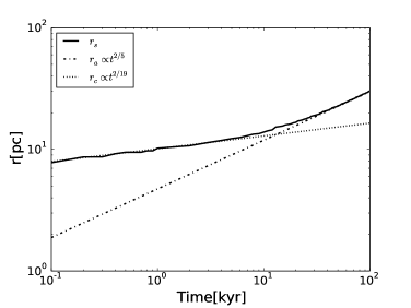
Figure 9: Evolution of the conduction/shock front in the point explosion simulation with isotropic conduction ($r_{s}$ – solid curve). The dotted line is the analytic expectation for a pure conduction problem ($r_{c}$), and the dot-dashed line plots the analytic expectation for the classic adiabatic Sedov-Taylor problem ($r_{a}$).

These results notably verify the accuracy and reliability of our conduction scheme on randomly oriented, moving meshes. They also validate the accuracy of the coupling between the hydrodynamics and heat conduction in our implementation.

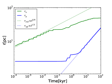
Figure 10: Evolution of the conduction/shock front in the point explosion simulation with anisotropic conduction in the direction of the magnetic field ($r_{x}$ – solid blue curve) and perpendicular to it ($r_{y}$ – solid green curve). Over-plotted is the analytic solution for the evolution of a pure conduction front in 1D ($r_{c1d}$ – dotted blue curve) and a pure adiabatic shock front in 2D ($r_{\rm cyl}$ – dotted green curve).

4.5 Convective instabilities in a rapidly conducting plasma

The dynamics of conducting plasmas differ from that of an adiabatic fluid (Balbus, 2000; Quataert, 2008). When the conduction timescale is much smaller than the dynamical time of the plasma (rapid conduction limit), the temperature gradient and the local orientation of the magnetic field determine the plasma’s convective stability. When the temperature increases with height, the convective instability is known as the heat-flux-driven buoyancy instability (HBI) and when it decreases with height it is described as magneto-thermal instability (MTI).

Balbus (2000) investigated weakly magnetized plasma with ${\rm d}T/{\rm d}z<0$ and identified that a small perturbation applied to a system in hydrostatic and thermal equilibrium can induce vigorous convection (MTI). In the rapid conduction regime, the gas is isothermal along the magnetic field lines. Since the temperature decreases with height, fluid elements displaced in the upward direction are warmer than their new surroundings, making them expand and rise. Similarly, fluid elements displaced in the downward direction sink. McCourt et al. (2011) showed that the MTI drives sustained turbulence for as long as the temperature gradient persists. The plasma never becomes stable, and the magnetic field and fluid velocities are nearly isotropic at late times.

Quataert (2008) showed that a stable system can become unstable even when ${\rm d}T/{\rm d}z>0$, in the presence of a background heat flux (HBI). This can happen if the magnetic fields lines are parallel to the temperature gradient. The regions of converging and diverging magnetic field lines fields correspond to regions where the plasma is locally heated and cooled. As a result, when ${\rm d}T/{\rm d}z>0$, a fluid element displaced downward is conductively cooled, making it colder than the surroundings and letting it sink further down. On the other hand, a fluid element displaced upwards becomes warmer than the surroundings and buoyantly rises. It was shown that HBI has the tendency to re-orient vertical magnetic fields into a horizontal configuration and can thus significantly reduce conductive heat transport in the system.

In this subsection, we present simulations of the MTI and HBI instabilities using our implementation of the anisotropic thermal conduction and compare our results to previous simulations performed by Parrish & Stone (2005), Parrish & Quataert (2008) and McCourt et al. (2011).

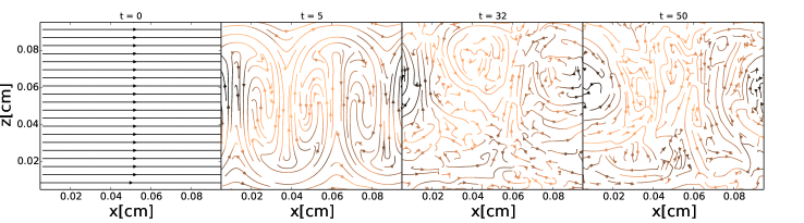
Figure 11: Evolution of the magnetic field in the MTI test simulation in 2D. We start with an initially horizontal magnetic field. The colours represent the magnetic field intensity at each point, with lighter colours depicting higher magnetic field strengths. The simulation time at the top of each panel is in units of the buoyancy timescale $t_{\rm buoy}\sim 1.7\,{\rm s}$.

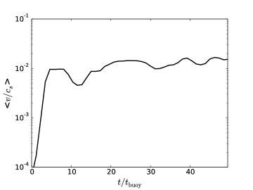
Figure 12: Evolution of the volume averaged Mach number of the turbulence generated in the MTI simulation.

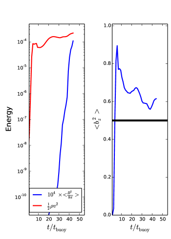
Figure 13: Left panel: Evolution of the kinetic (red curve) and magnetic (blue curve) energy in the MTI simulation. Right panel: Evolution of the orientation of the magnetic field in the same simulation.

4.5.1 Simulation of the MTI

We perform a 2D simulation of the MTI instability. This simulation is local in the sense that the domain size $L$ is much smaller than the plasma scale height $H$. We start with a stable system in hydrostatic and thermal equilibrium. The gravitational force field is ${\bf g}=-g_{0}{\bf\hat{z}}$, with $g_{0}=1\ \rm{cm\,s^{-2}}$. The internal energy, density and the pressure profiles are set-up as in the local simulations of Parrish & Stone (2005),

$$\begin{split}u&=u_{0}(1-z/H),\\ \rho&=\rho_{0}(1-z/H)^{2},\\ P&=P_{0}(1-z/H)^{3},\\ \end{split}$$ (48)

where $u_{0}=1.5\ \rm{erg\,g^{-1}}$, $\rho_{0}=1\ \rm{g\,cm^{-3}}$, $P_{0}=1\ \rm{dyne\,cm^{-2}}$ and $H=3$. We set the adiabatic index to $\gamma=5/3$. The size of the computational domain is $(0.1\ \rm{cm})^{2}$, which corresponds to $L/H=1/30$. The resolution is $100^{2}$ particles. The diffusivity is set to $\chi=0.01\ \rm{cm^{2}\,s^{-1}}$. The initial magnetic field is set to ${\bf B}=\{1,0\}\ \rm{nG}$.

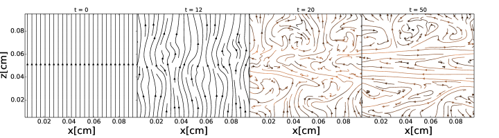
Figure 14: Same as Fig. 11, but for the HBI simulation. The buoyancy time for this simulation is $t_{\rm{buoy}}\sim 1.4\,{\rm s}$.

We use reflective boundary conditions. The temperature at the upper and lower boundaries are constant, meaning that they act as sources/sinks of heat during the simulation. The density at the boundary is extrapolated from the cells below, such that they maintain hydrostatic equilibrium throughout the duration of the simulation. This extrapolation along with the reflecting boundary conditions influence the evolution of the instability. To reduce this effect we sandwich the anisotropically conducting region between isotropic buoyantly neutral layers as in Parrish & Stone (2005). The domain is divided into three equal regions of length $L/3$, and the top and bottom layers have isotropic conduction, while the middle layer has fully anisotropic heat transport. The setup has a positive entropy gradient meaning that the system is stable in the absence of anisotropic conduction. All the results for the MTI are quoted for quantities within the anisotropic conduction region. An initial velocity perturbation of the from

$$v_{z}=10^{-4}c_{s}\sin\left(\frac{4\pi x}{L}\right)$$ (49)

is applied. We run this simulation setup with MHD and heat conduction until $t=50\ t_{\rm buoy}$, where $t_{\rm buoy}=\omega_{\rm buoy}^{-1}=|g\ \delta\ln T/\delta z|^{-1/2}\sim 1.7\,{\rm s}$.

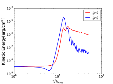
Figure 15: Evolution of the vertical (blue curve) and horizontal (red curve) kinetic energy in the HBI simulation. The kinetic energy is in units of ${\rm erg\,cm^{-3}}$ and the time is in units of $t_{\rm buoy}\sim 1.4\,{\rm s}$.

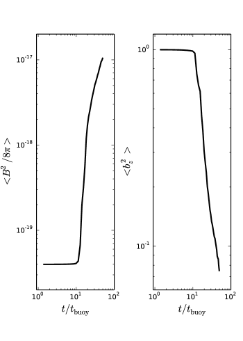
Figure 16: The panel on the left hand side shows the increase of the magnetic energy in the HBI simulation, while the right hand side panel plots the evolution of the orientation of the magnetic field.

Fig. 11 shows the orientation of the magnetic field lines as a function of time. Initially the magnetic fields are horizontal. Within $5\,t_{\rm buoy}$ the system becomes unstable and the magnetic field is dragged along rising and sinking parcels of gas making it nearly vertical. Quataert (2008) showed that the maximum growth rate of the MTI goes to zero when $\hat{b}_{z}=1$. One would therefore expect the instability to saturate at this point. This is however not the case. McCourt et al. (2011) showed that the displacements orthogonal to gravity generate a horizontal magnetic field component from the vertical magnetic field. This further seeds the instability and closes the dynamo loop. Therefore, this process continuously drives the MTI and sustains turbulence. This is only true due to the constant temperature boundary conditions that are imposed. If the temperatures were free to vary, the MTI could saturate by making the plasma isothermal.

Figure 12 shows the volume-averaged Mach number within the anisotropic region of the simulation domain as a function of time. The increase of the average Mach number is due to MTI-driven turbulence. The value of the average Mach number is quite similar to the value obtained by McCourt et al. (2011) in their local 3D MTI simulation. Of course, the Mach number is suppressed due to the small size of the domain, increasing the domain size can potentially induce turbulence of the order of the sound speed $v\sim c_{s}$.

The left hand panel of Fig. 13 shows the kinetic (red curve) and magnetic (blue curve) energies as a function of time. The figure clearly demonstrates the non-linear amplification of the magnetic field due to the turbulence generated by the MTI. The kinetic energy increases rapidly at early times and then slowly saturates after about $5\,t_{\rm buoy}$, while the magnetic field is amplified exponentially and will only saturate once it reaches equipartition. The simulation needs to be run for a very long time in order to see the saturation of the magnetic field.

The right hand panel of Fig. 13 shows the evolution of the orientation of the magnetic field as a function of time. Initially the magnetic fields get stretched into an almost vertical configuration. The persistent convective turbulence then drives down the value of $\hat{b}_{z}$, making it asymptote to the isotropic value. These results are quantitatively and qualitatively similar to the results obtained in the simulations of McCourt et al. (2011).

4.5.2 Simulation of HBI

Finally, we perform local 2D simulations of the HBI. The values for the domain size, resolution, heat conduction coefficient and gravity are the same as the ones used in the MTI simulations. We also use the same boundary conditions. The internal energy, density and pressure profiles are set to

$$\begin{split}u&=u_{0}(1+z/H),\\ \rho&=\rho_{0}/(1+z/H)^{3},\\ P&=P_{0}/(1+z/H)^{2},\\ \end{split}$$ (50)

with $u_{0}=1.5\ \rm{erg\,g^{-1}}$, $\rho_{0}=1\ \rm{g\,cm^{-3}}$, $P_{0}=1\,\rm{dyne\,cm^{-2}}$ and $H=2$. This corresponds to $L/H=0.05$ and $t_{\rm buoy}\sim 1.4\,{\rm s}$. The magnetic field is initialised to ${\bf B}=\{0,1\}\,{\rm nG}$. Quataert (2008) showed that non-zero $\hat{k}_{x}$ and $\hat{k}_{z}$, generated converging and diverging field lines that triggered HBI. Therefore the initial perturbation is set to

$${\bf v}=10^{-4}c_{s}\left[\sin\left(\frac{3\pi y}{L}\right)\hat{i}+\sin\left(\frac{4\pi x}{L}\right)\hat{k}\right].$$ (51)

As in the previous subsection, all the results for the HBI are quoted for quantities within the anisotropic conduction region. Fig. 14 shows the orientation of the magnetic fields as a function of time. By $t=10\,t_{\rm buoy}$, the magnetic field lines get perturbed enough that there are regions where they converge or diverge. These correspond to regions where the plasma is locally heated and cooled. As a result, when ${\rm d}T/{\rm d}z>0$, a fluid element displaced downward is conductively cooled via the background heat flux, making it colder than the surroundings and therefore letting it sink further down. On the other hand, a fluid element with an upward displacement gains energy, becomes warmer than the surroundings and buoyantly rises. The evolution becomes non-linear by $t\sim 12\,t_{\rm buoy}$. Afterwards the instability saturates and the magnetic field settles into an almost horizontal configuration by $t=50\,t_{\rm buoy}$.

This behaviour can be more clearly seen in Fig. 15, which shows the evolution of the vertical (blue curve) and horizontal (red curve) kinetic energy components as a function of time. During the linear growth phase of the instability, both components of the velocity field accelerate to equipartition with each other, which takes place at about $t\sim 12\,t_{\rm buoy}$. As the instability saturates the plasma becomes buoyantly stable and suppresses vertical motions whereas the horizontal motions continue unperturbed.

The left panel of Fig. 16 shows the evolution of the mean magnetic field energy as a function of time. The linear growth ends at $t\sim 12\,t_{\rm buoy}$, and most of the evolution of the magnetic field happens afterwards. This evolution is driven by the horizontal motions which both amplify and reorient the magnetic field. After a brief period of exponential growth, the field amplification is roughly linear in time. The right panel of Fig. 16 shows the evolution of the magnetic field orientation as a function of time. As expected, the HBI converts vertical magnetic fields into horizontal ones. Quantitatively, we expect that $\hat{b}_{z}\propto t^{-1}$, which is quite close to the value $\hat{b}_{z}\propto t^{-0.86}$ obtained in our simulation. The reorienting of the magnetic field also has the effect of severely reducing the conductive heat flux through the plasma. Stretching the field lines in this manner amplifies the field, and in our simulations the magnetic field strength is given by $B^{2}\propto t^{1.83}$, which is again close to the expected value of $B^{2}\propto t^{2}$. The saturated state of the HBI is buoyantly stable. We reiterate previous results and state that the HBI has the tendency to insulate conductive and convective transport in plasmas, which may significantly reduce the amount of conductive heat transport in clusters of galaxies.

5 Conclusions

In this work, we have presented an implementation of an extremum preserving anisotropic diffusion solver that works well on the unstructured moving mesh of Arepo. The method relies on splitting the one-sided facet fluxes into normal and oblique components and on limiting the oblique fluxes such that the method is locally conservative and also extremum preserving. The scheme makes use of harmonic averaging points and proposes a very simple yet robust interpolation scheme that works well for strong heterogeneous and anisotropic diffusion problems. In addition, the required discretisation stencil is essentially small. We also present efficient fully implicit and semi-implicit time integration schemes in order to overcome the restrictive nature of the diffusion time step, which arise due to the $\Delta x^{2}$ dependance of the von Neumann stability condition.

We have tested this implementation on a variety of numerical problems. The method works really well overall and reproduces analytic results very well in the test of the diffusion of a temperature step function. The main drawback of the method seems to be that the convergence order for highly anisotropic problems like the diffusion of a hot patch of gas in a circular magnetic field is only about $\sim 0.4-0.5$. In future work, we will try to improve upon this by choosing higher order interpolation schemes. Coming up with a less restrictive flux limiter should also help. We also verify that the numerical perpendicular diffusion is about $10^{-3}$ for $\Delta x/L\sim 0.01$, comparable to the values obtained by other methods (Sharma & Hammett, 2007). We also obtain a good numerical convergence rate for the perpendicular diffusion, of the order of $1.5$.

We have also verified the accuracy and robustness of the code when conduction and hydrodynamics are coupled by simulating point explosions with isotropic and anisotropic heat conduction. We show that the point explosion test with isotropic heat conduction can be split into two regimes, the conduction dominated regime and the advection dominated regime. Conduction dominates at early times and accelerates the shock front beyond the classical Sedov solution. At late times, the hydrodynamic forces take over and the position of the shock front returns to that of the Sedov solution. The temperature profile behind the shock front is much shallower than the adiabatic case. This has consequences, for example, for observations attempting to diagnose hot winds with X-ray radiation. In particular, Strickland et al. (1997) find a flat temperature gradient potentially consistent with our simulations in the M82 superwind on kpc scales.

We also a perform Sedov blast wave explosion test with anisotropic thermal conduction. Initially, the conduction front races along the magnetic field while there is very little advection perpendicular to it. The position of the conduction front along the magnetic field accurately follows the solution of a 1D conduction problem. At late times, the advection perpendicular to the magnetic field decelerates the conduction front. This also means that the geometry of the problem changes from a spherical to a cylindrical shock. When advection does start to dominate, the simulation accurately follows the cylindrical Sedov solution. We conclude that the ISM magnetic fields play an important role in the evolution of SN remnants.

Finally, we simulate convective instabilities induced by anisotropic conduction in a rapidly conducting plasma. We simulate the magneto-thermal and heat-flux-driven buoyancy instability in 2D and verify the results of Parrish & Stone (2005); Parrish & Quataert (2008); McCourt et al. (2011). We find that, in the MTI, the initially horizontal magnetic field is quickly disrupted, the system becomes unstable and the magnetic field is dragged along rising and sinking parcels of gas making the field orientation nearly vertical. Horizontal displacements makes the system non-linearly unstable to the MTI thereby generating horizontal magnetic fields and so on. At late times the magnetic field is completely randomised. This turbulence also increases the magnetic and the kinetic energy of the gas and thus generates additional pressure support against gravity. This pressure support might become important, especially in cluster environments (McCourt et al., 2013). We also simulate HBI instability and get similar B field magnification and KE increase values as previous simulations. However, the HBI quietly saturates when the magnetic field becomes horizontal. Therefore, HBI tends to hinder conductive transport in clusters.

To summarise, we have implemented an efficient, robust, extremum preserving anisotropic thermal conduction solver in Arepo. This algorithm can be easily generalized to simulate other interesting astrophysical diffusion processes as well, such as cosmic ray diffusion (Pfrommer, 2013) or radiative transfer problems. In the latter case, it can be used for moment-based radiative transfer calculations (such as in Gnedin & Abel 2001; Petkova & Springel 2009; Rosdahl & Teyssier 2015) where the anisotropic diffusion tensor is replaced by a local Eddington tensor, encoding information about the preferred local propagation direction of the photons from a set of discrete sources.

In forthcoming work, we plan to use the implementation introduced here to study timely problems in astrophysics related to conduction, such as heat transport in clusters, the evolution of supernova remnants, role of convective instabilities in galaxy clusters, and the distribution of heat from AGN jets into the ICM. An extension to cosmic ray transport is another obvious research direction where the anisotropic diffusion solver could be fruitfully applied.

References

- Aavatsmark et al. (1996) Aavatsmark I., Barkve T., Bøe Ø., Mannseth T., 1996, Journal of Computational Physics, 127, 2
- Agelas et al. (2009) Agelas L., Eymard R., Herbin R., 2009, Comptes Rendus Mathematique, 347, 673
- Arth et al. (2014) Arth A., Dolag K., Beck A. M., Petkova M., Lesch H., 2014, preprint, (arXiv:1412.6533)
- Balbus (2000) Balbus S. A., 2000, ApJ, 534, 420
- Balsara et al. (2008a) Balsara D. S., Tilley D. A., Howk J. C., 2008a, MNRAS, 386, 627
- Balsara et al. (2008b) Balsara D. S., Bendinelli A. J., Tilley D. A., Massari A. R., Howk J. C., 2008b, MNRAS, 386, 642
- Barenblatt & Cole (1981) Barenblatt G. I., Cole J. D., 1981, Journal of Applied Mechanics, 48, 213
- Booth et al. (2013) Booth C. M., Agertz O., Kravtsov A. V., Gnedin N. Y., 2013, ApJ, 777, L16
- Breil & Maire (2007) Breil J., Maire P.-H., 2007, Journal of Computational Physics, 224, 785
- Cowie & McKee (1977) Cowie L. L., McKee C. F., 1977, ApJ, 211, 135
- De Smedt et al. (2010) De Smedt B., Pattyn F., De Groen P., 2010, Journal of Glaciology, 56, 257
- Dembo et al. (1982) Dembo R. S., Eisenstat S. C., Steihaug T., 1982, SIAM Journal on Numerical Analysis, 19, 400
- Dubois & Commerçon (2015) Dubois Y., Commerçon B., 2015, preprint, (arXiv:1509.07037)
- Eymard et al. (2012) Eymard Guichard, Cindy Herbin, Raphaèle 2012, ESAIM: M2AN, 46, 265
- Falgout & Yang (2002) Falgout R. D., Yang U. M., 2002, in Proceedings of the International Conference on Computational Science-Part III. ICCS ’02. Springer-Verlag, London, UK, UK, pp 632–641, http://dl.acm.org/citation.cfm?id=645459.653635
- Fanchi (2005) Fanchi J. R., 2005, Principles of Applied Reservoir Simulation. Gulf Professional Publishing
- Fermi (1949) Fermi E., 1949, Physical Review, 75, 1169
- Gao & Wu (2013) Gao Z., Wu J., 2013, Journal of Computational Physics, 250, 308
- Giataganas & Soltanpanahi (2014) Giataganas D., Soltanpanahi H., 2014, Journal of High Energy Physics, 6, 47
- Ginzburg et al. (1980) Ginzburg V. L., Khazan I. M., Ptuskin V. S., 1980, Ap&SS, 68, 295
- Gnedin & Abel (2001) Gnedin N. Y., Abel T., 2001, New Astron., 6, 437
- Henson & Yang (2002) Henson V. E., Yang U. M., 2002, Applied Numerical Mathematics, 41, 155
- Jubelgas et al. (2008) Jubelgas M., Springel V., Enßlin T., Pfrommer C., 2008, A&A, 481, 33
- McCourt et al. (2011) McCourt M., Parrish I. J., Sharma P., Quataert E., 2011, MNRAS, 413, 1295
- McCourt et al. (2013) McCourt M., Quataert E., Parrish I. J., 2013, MNRAS, 432, 404
- Mocz et al. (2015) Mocz P., Vogelsberger M., Pakmor R., Genel S., Springel V., Hernquist L., 2015, MNRAS, 452, 3853
- Pakmor & Springel (2013) Pakmor R., Springel V., 2013, MNRAS, 432, 176
- Pakmor et al. (2016) Pakmor R., Springel V., Bauer A., Mocz P., Munoz D. J., Ohlmann S. T., Schaal K., Zhu C., 2016, MNRAS, 455, 1134
- Parrish & Quataert (2008) Parrish I. J., Quataert E., 2008, ApJ, 677, L9
- Parrish & Stone (2005) Parrish I. J., Stone J. M., 2005, ApJ, 633, 334
- Pawar et al. (2014) Pawar N., Donth C., Weiss M., 2014, Current Biology, 24, 1905
- Pert (1981) Pert G., 1981, Journal of Computational Physics, 42, 20
- Petkova & Springel (2009) Petkova M., Springel V., 2009, MNRAS, 396, 1383
- Pfrommer (2013) Pfrommer C., 2013, ApJ, 779, 10
- Potier (2005) Potier C. L., 2005, Comptes Rendus de l’Academie des Sciences, 1, 787
- Powell et al. (1999) Powell K. G., Roe P. L., Linde T. J., Gombosi T. I., De Zeeuw D. L., 1999, Journal of Computational Physics, 154, 284
- Price (2007) Price D. J., 2007, Publ. Astron. Soc. Australia, 24, 159
- Quataert (2008) Quataert E., 2008, ApJ, 673, 758
- Rasera & Chandran (2008) Rasera Y., Chandran B., 2008, ApJ, 685, 105
- Reinicke & Meyer-Ter-Vehn (1991) Reinicke P., Meyer-Ter-Vehn J., 1991, Physics of Fluids, 3, 1807
- Rosdahl & Teyssier (2015) Rosdahl J., Teyssier R., 2015, MNRAS, 449, 4380
- Saad & Schultz (1986) Saad Y., Schultz M. H., 1986, SIAM Journal on Scientific and Statistical Computing, 7, 856
- Sarazin (1988) Sarazin C. L., 1988, X-ray emission from clusters of galaxies
- Schlickeiser (2002) Schlickeiser R., 2002, Cosmic Ray Astrophysics
- Sedov (1959) Sedov L. I., 1959, Similarity and Dimensional Methods in Mechanics
- Sharma & Hammett (2007) Sharma P., Hammett G. W., 2007, Journal of Computational Physics, 227, 123
- Sharma & Hammett (2011) Sharma P., Hammett G. W., 2011, Journal of Computational Physics, 230, 4899
- Sharma et al. (2008) Sharma P., Quataert E., Stone J. M., 2008, MNRAS, 389, 1815
- Sheng & Yuan (2011) Sheng Z., Yuan G., 2011, Journal of Computational Physics, 230, 2588
- Sheng & Yuan (2012) Sheng Z., Yuan G., 2012, Journal of Computational Physics, 231, 3739
- Shestakov (1999) Shestakov A. I., 1999, Physics of Fluids, 11, 1091
- Sovinec et al. (2004) Sovinec C., et al., 2004, Journal of Computational Physics, 195, 355
- Spitzer (1962) Spitzer L., 1962, Physics of Fully Ionized Gases
- Springel (2010) Springel V., 2010, MNRAS, 401, 791
- Strickland et al. (1997) Strickland D. K., Ponman T. J., Stevens I. R., 1997, A&A, 320, 378
- Thompson et al. (2015) Thompson T. A., Quataert E., Zhang D., Weinberg D., 2015, preprint, (arXiv:1507.04362)
- Vogelsberger et al. (2012) Vogelsberger M., Sijacki D., Kereš D., Springel V., Hernquist L., 2012, MNRAS, 425, 3024
- Voit (2011) Voit G. M., 2011, ApJ, 740, 28
- Voit & Donahue (2015) Voit G. M., Donahue M., 2015, ApJ, 799, L1
- Voit et al. (2008) Voit G. M., Cavagnolo K. W., Donahue M., Rafferty D. A., McNamara B. R., Nulsen P. E. J., 2008, ApJ, 681, L5
- Voit et al. (2015) Voit G. M., Donahue M., Bryan G. L., McDonald M., 2015, Nature, 519, 203
- Weickert et al. (1998) Weickert J., Romeny B. M. T. H., Viergever M. A., 1998, IEEE Transactions on Image Processing, 7, 398
- Yuan & Sheng (2008) Yuan G., Sheng Z., 2008, Journal of Computational Physics, 227, 6288
- Zakamska & Narayan (2003) Zakamska N. L., Narayan R., 2003, ApJ, 582, 162
- Zeldovich & Raizer (1966) Zeldovich Y. B., Raizer Y. P., 1966, Elements of gasdynamics and the classical theory of shock waves