RSG: Beating Subgradient Method without Smoothness and Strong Convexity

Abstract

In this paper, we study the efficiency of a Restarted SubGradient (RSG) method that periodically restarts the standard subgradient method (SG). We show that, when applied to a broad class of convex optimization problems, RSG method can find an $\epsilon$-optimal solution with a lower complexity than the SG method. In particular, we first show that RSG can reduce the dependence of SG’s iteration complexity on the distance between the initial solution and the optimal set to that between the $\epsilon$-level set and the optimal set multiplied by a logarithmic factor. Moreover, we show the advantages of RSG over SG in solving three different families of convex optimization problems. (a) For the problems whose epigraph is a polyhedron, RSG is shown to converge linearly. (b) For the problems with local quadratic growth property in the $\epsilon$-sublevel set, RSG has an $O(\frac{1}{\epsilon}\log(\frac{1}{\epsilon}))$ iteration complexity. (c) For the problems that admit a local Kurdyka-Łojasiewicz property with a power constant of $\beta\in[0,1)$, RSG has an $O(\frac{1}{\epsilon^{2\beta}}\log(\frac{1}{\epsilon}))$ iteration complexity. The novelty of our analysis lies at exploiting the lower bound of the first-order optimality residual at the $\epsilon$-level set. It is this novelty that allows us to explore the local properties of functions (e.g., local quadratic growth property, local Kurdyka-Łojasiewicz property, more generally local error bound conditions) to develop the improved convergence of RSG. We also develop a practical variant of RSG enjoying faster convergence than the SG method, which can be run without knowing the involved parameters in the local error bound condition. We demonstrate the effectiveness of the proposed algorithms on several machine learning tasks including regression, classification and matrix completion.

Keywords: subgradient method, improved convergence, local error bound, machine learning

1 Introduction

We consider the following generic optimization problem

$$f_{*}:=\min_{\mathbf{w}\in\Omega}f(\mathbf{w})$$ (1)

where $f:\mathbb{R}^{d}\rightarrow(-\infty,+\infty]$ is an extended-valued, lower semicontinuous and convex function, and $\Omega\subseteq\mathbb{R}^{d}$ is a closed convex set such that $\Omega\subseteq\text{dom}(f)$. Here, we do not assume the smoothness of $f$ on $\text{dom}(f)$. During the past several decades, many fast (especially linearly convergent) optimization algorithms have been developed for (1) when $f$ is smooth and/or strongly convex. On the contrary, there are relatively fewer techniques for solving generic non-smooth and non-strongly convex optimization problems which still have many applications in machine learning, statistics, computer vision, and etc. To solve (1) with $f$ being potentially non-smooth and non-strongly convex, one of the simplest algorithms to use is the subgradient (SG)  method. When $f$ is Lipschitz-continuous, it is known that SG method requires $O(1/\epsilon^{2})$ iterations for obtaining an $\epsilon$-optimal solution (Rockafellar, 1970; Nesterov, 2004). It has been shown that this iteration complexity is unimprovable for general non-smooth and non-strongly convex problems in a black-box first-order oracle model of computation (Nemirovsky A.S. and Yudin, 1983). However, better iteration complexity can be achieved by other first-order algorithms for certain classes of $f$ where additional structural information is available (Nesterov, 2005; Gilpin et al., 2012; Freund and Lu, 2017; Renegar, 2014, 2015, 2016).

In this paper, we present a generic restarted subgradient (RSG) method for solving (1) which runs in multiple stages with each stage warm-started by the solution from the previous stage. Within each stage, the standard projected subgradient descent is performed for a fixed number of iterations with a constant step size. This step size is reduced geometrically from stage to stage. With these schemes, we show that RSG can achieve a lower iteration complexity than the classical SG method when $f$ belongs to some classes of functions. In particular, we summarize the main results and properties of RSG below:

• For the general problem (1), under mild assumptions (see Assumption 1), RSG has an iteration complexity of $O(\frac{1}{\epsilon^{2}}\log(\frac{\epsilon_{0}}{\epsilon}))$ which has an addition $\log(\frac{\epsilon_{0}}{\epsilon})$  term but has significantly smaller constant in $O(\cdot)$ compared to SG. In particular, compared with SG whose iteration complexity linearly depends on the distance from the initial solution to the optimal set, RSG’s iteration complexity only has a linear dependence on the distance from the $\epsilon$-level set to the optimal set, which is much smaller than the distance from the initial solution to the optimal set. Its dependence on the initial solution is through $\epsilon_{0}$ - a known upper bound of the initial optimality gap, which only scales logarithmically.

• When $f$ is locally quadratically growing (see Definition 10), which is a weaker condition than strong convexity, RSG can achieve an $O(\frac{1}{\epsilon}\log(\frac{1}{\epsilon}))$ iteration complexity.

• When $f$ admits a local Kurdyka-Łojasiewicz property (see Definition 13) with a power desingularizing function of degree $1-\beta$ where $\beta\in[0,1)$, RSG can achieve an $O(\frac{1}{\epsilon^{2\beta}}\log(\frac{1}{\epsilon}))$ complexity.

• When the epigraph of $f$ over $\Omega$ is a polyhedron, RSG can achieve linear convergence, i.e., an $O(\log(\frac{1}{\epsilon}))$ iteration complexity.

These results, except for the first one, are derived from a generic complexity of RSG for the problem satisfying a local error condition (15), which has a close connection to the existing error bound conditions and growth conditions (Pang, 1997, 1987; Luo and Tseng, 1993; Necoara et al., 2015; Bolte et al., 2006) in the literature. In spite of its simplicity, the analysis of RSG provides additional insight on improving first-order methods’ iteration complexity via restarting. It is known that restarting can improve the theoretical complexity of (stochastic) SG method for non-smooth problems when strongly convexity is assumed (Ghadimi and Lan, 2013; Chen et al., 2012; Hazan and Kale, 2011) but we show that restarting can be still helpful for SG methods under other (weaker) assumptions. We would like to remark that the key lemma (Lemma 4) developed in this work can be leveraged to develop faster algorithms in different contexts. For example, built on the groundwork laid in this paper, Xu et al. (2016) have developed new smoothing algorithms to improve the convergence of Nesterov’s smoothing algorithm (Nesterov, 2005) for non-smooth optimization with a special structure, and Xu et al. (2017) have developed new stochastic gradient methods to improve the convergence of standard stochastic subgradient method.

We organize the reminder of the paper as follows. Section 2 reviews some related work. Section 3 presents some preliminaries and notations. Section 4 presents the algorithm of RSG and the general theory of convergence. Section 5 considers several classes of non-smooth and non-strongly convex problems and shows the improved iteration complexities of RSG. Section 6 presents parameter-free variants of RSG. Section 8 presents some experimental results. Finally, we conclude in Section 9.

2 Related Work

Smoothness and strong convexity are two key properties of a convex optimization problem that affect the iteration complexity of finding an $\epsilon$-optimal solution by first-order methods. In general, a lower iteration complexity is expected when the problem is either smooth or strongly convex. We refer the reader to (Nesterov, 2004; Nemirovsky A.S. and Yudin, 1983) for the optimal iteration complexity of first-order methods when applied to the problems with different properties of smoothness and convexity. Recently there has emerged a surge of interest in further accelerating first-order methods for non-strongly convex or non-smooth problems that satisfy some particular conditions (Bach and Moulines, 2013; Wang and Lin, 2014; So and Zhou, 2017; Hou et al., 2013; Zhou et al., 2015; Gong and Ye, 2014; Gilpin et al., 2012; Freund and Lu, 2017). The key condition for us to develop an improved complexity is a local error bound condition (15) which is closely related to the error bound conditions in (Pang, 1987, 1997; Luo and Tseng, 1993; Necoara et al., 2015; Bolte et al., 2006; Zhang, 2016).

Various error bound conditions have been exploited in many studies to analyze the convergence of optimization algorithms. For example, Luo and Tseng (1992a, b, 1993) established the asymptotic linear convergence of a class of feasible descent algorithms for smooth optimization, including coordinate descent method and projected gradient method, based on a local error bound condition. Their results on coordinate descent method were further extended for a more general class of objective functions and constraints in (Tseng and S., 2009a, b). Wang and Lin (2014) showed that a global error bound holds for a family of non-strongly convex and smooth objective functions for which feasible descent methods can achieve a global linear convergence rate. Recently, these error bounds have been generalized and leveraged to show faster convergence for structured convex optimization that consists of a smooth function and a simple non-smooth function (Hou et al., 2013; Zhou and So, 2017; Zhou et al., 2015). Recently, Necoara and Clipici (2016) considered a generalized error bound condition, and established linear convergence of a parallel version of a randomized (block) coordinate descent method for minimizing the sum of a partially separable smooth convex function and a fully separable non-smooth convex function. We would like to emphasize that the aforementioned error bounds are different from the local error bound explored in this paper. In particular, they bound the distance of a point to the optimal set by using the norm of the projected gradient or proximal gradient at the point, thus requiring the smoothness of the objective function. In contrast, we bound the distance of a point to the optimal set by its objective residual with respect to the optimal value, covering a much broader family of functions. More recently, there have appeared many studies that consider smooth optimization or composite smooth optimization problems whose objective functions satisfy different error bound conditions, growth conditions or other non-degeneracy conditions and established the linear convergence rates of several first-order methods including proximal-gradient method, accelerated gradient method, prox-linear method and so on (Gong and Ye, 2014; Necoara et al., 2015; Zhang and Cheng, 2015; Zhang, 2016; Karimi et al., 2016; Drusvyatskiy and Lewis, 2018; Drusvyatskiy and Kempton, 2016; Hou et al., 2013; Zhou et al., 2015). The relative strength and relationships between some of those conditions are studied by Necoara et al. (2015) and Zhang (2016). For example, Necoara et al. (2015) showed that under the smoothness assumption the second-order growth condition (i.e., the considered error bound condition in the present work with $\theta=1/2$) is equivalent to the error bound condition in (Wang and Lin, 2014). It was brought to our attention that the local error bound condition in the present paper is closely related to metric subregularity of subdifferentials (Artacho and Geoffroy, 2008; Kruger, 2015; Drusvyatskiy et al., 2014; Mordukhovich and Ouyang, 2015).

Gilpin et al. (2012) established a polyhedral error bound condition for problems whose epigraph is polyhedral and domain is a bounded polytope. Using this polyhedral error bound condition, they studied a two-person zero-sum game and proposed a restarted first-order method based on Nesterov’s smoothing technique (Nesterov, 2005) that can find the Nash equilibrium and has linear convergence rate. The differences between (Gilpin et al., 2012) and this work are: (i) we study subgradient methods instead of Nesterov’s smoothing technique, where the former have broader applicability than Nesterov’s smoothing technique; (ii) our linear convergence can be derived for a slightly general problem where the domain is allowed to be an unbounded polyhedron as long as the polyhedral error bound condition in Lemma 8 holds, which is the case for many important applications; (iii) we consider a general condition that subsumes the polyhedral error bound condition as a special case and we try to solve the general problem (1) rather than the bilinear saddle-point problem in (Gilpin et al., 2012).

The error bound condition that allows us to derive a linear convergence of RSG is the same to the weak sharp minimum condition, which was first coined in 1970s (Polyak, 1979). However, it was used even earlier for studying the convergence of subgradient method (Eremin, 1965; Polyak, 1969). Later, it was studied in many subsequent works (Polyak, 1987; Burke and Ferris., 1993; Studniarski and Ward, 1999; Ferris, 1991; Burke and Deng, 2002, 2005, 2009). Finite or linear convergence of several algorithms has been established under the weak sharp minimum condition, including gradient projection method (Polyak, 1987), the proximal point algorithm (PPA) (Ferris, 1991), and subgradient method with a particular choice of step size (see below) (Polyak, 1969). We would like to emphasize the differences between the results in these works and the results in the present work that make our results novel: (i) the gradient projection method and its finite convergence established in (Polyak, 1987) requires the gradient of the objective function to be Lipschitz continuous, i.e., the objective function is smooth (please refer to Theorem 1 (Chapter 7, pp 207) in (Polyak, 1987)), in contrast we do not assume smoothness of the objective function; (ii) the PPA studied in (Ferris, 1991) requires solving a proximal sub-problem consisting of the original objective function and a strongly convex function at every iteration, and therefore its finite convergence does not mean that only a finite number of subgradient evaluations is needed. In contrast, the linear convergence in this paper was in terms of the number of subgradient evaluations; (iii) linear convergence of a subgradient method studied in (Polyak, 1969) requires knowing the optimal objective value for setting its step size, and its convergence is in terms of the distance of the iterates to the optimal set, which is weaker than our linear convergence in terms of objective gap. In addition, our method does not require knowing the optimal objective value. Instead the basic variant of RSG that has a linear convergence only needs to know the value of the multiplicative constant parameter in the local error bound condition. For problems without knowing this parameter, we also develop a practical variant of RSG that can achieve a convergence rate close to linear convergence.

In his recent work (Renegar, 2014, 2015, 2016), Renegar presented a framework of applying first-order methods to general conic optimization problems by transforming the original problem into an equivalent convex optimization problem with only linear equality constraints and a Lipschitz-continuous objective function. This framework greatly extends the applicability of first-order methods to the problems with general linear inequality constraints and leads to new algorithms and new iteration complexity. One of his results related to this work is Corollary 3.4 of (Renegar, 2015), which implies, if the objective function has a polyhedral epigraph and the optimal objective value is known beforehand, a subgradient method can have a linear convergence rate. Compared to this result of his, our method does not need to know the optimal objective value. Note that Renegar’s method can be applied in a general setting where the objective function is not necessarily polyhedral while our method obtains improved iteration complexities under the local error bound conditions.

More recently, Freund and Lu (2017) proposed a new SG method by assuming that a strict lower bound of $f_{*}$, denoted by $f_{slb}$, is known and $f$ satisfies a growth condition, $\|\mathbf{w}-\mathbf{w}^{*}\|_{2}\leq\mathcal{G}\cdot(f(\mathbf{w})-f_{slb})$, where $\mathbf{w}^{*}$ is the optimal solution closest to $\mathbf{w}$ and $\mathcal{G}$ is a growth rate constant depending on $f_{slb}$. Using a novel step size that incorporates $f_{slb}$, for non-smooth optimization, their SG method achieves an iteration complexity of $O(\mathcal{G}^{2}(\frac{\log H}{\epsilon^{\prime}}+\frac{1}{\epsilon^{\prime 2}}))$ for finding a solution $\hat{\mathbf{w}}$ such that $f(\hat{\mathbf{w}})-f_{*}\leq\epsilon^{\prime}(f_{*}-f_{slb})$, where $H=\frac{f(\mathbf{w}_{0})-f_{slb}}{f_{*}-f_{slb}}$ and $\mathbf{w}_{0}$ is the initial solution. We note that there are several key differences in the theoretical properties and implementations between our work and (Freund and Lu, 2017): (i) Their growth condition has a similar form to the inequality (7) we prove for a general function but there are still noticeable differences in the both sides and the growth constants. (ii) The convergence results in (Freund and Lu, 2017) are established based on finding an solution $\hat{\mathbf{w}}$ with a relative error of $\epsilon^{\prime}$ while we consider absolute error. (iii) By rewriting the convergence results in (Freund and Lu, 2017) in terms of absolute accuracy $\epsilon$ with $\epsilon=\epsilon^{\prime}(f_{*}-f_{slb})$, the complexity in (Freund and Lu, 2017) depends on $f_{*}-f_{slb}$ and may be higher than ours if $f_{*}-f_{slb}$ is large. However, Freund and Lu’s new SG method is still attractive due to that it is a parameter free algorithm without requiring the value of the growth constant $\mathcal{G}$. We will compared our RSG method with the method in (Freund and Lu, 2017) with more details in Section 7.

Restarting and multi-stage strategies have been utilized to achieve the (uniformly) optimal theoretical complexity of (stochastic) SG methods when $f$ is strongly convex (Ghadimi and Lan, 2013; Chen et al., 2012; Hazan and Kale, 2011) or uniformly convex (Juditsky and Nesterov, 2014). Here, we show that restarting can be still helpful even without uniform or strong convexity. Furthermore, in all the algorithms proposed in (Ghadimi and Lan, 2013; Chen et al., 2012; Hazan and Kale, 2011; Juditsky and Nesterov, 2014), the number of iterations per stage increases between stages while our algorithm uses the same number of iterations in all stages. This provides a different possibility of designing restarted algorithms for a better complexity only under a local error bound condition.

3 Preliminaries

In this section, we define some notations used in this paper and present the main assumptions needed to establish our results. We use $\partial f(\mathbf{w})$ to denote the set of subgradients (the subdifferential) of $f$ at $\mathbf{w}$. Since the objective function is not necessarily strongly convex, the optimal solution is not necessarily unique. We denote by $\Omega_{*}$ the optimal solution set and by $f_{*}$ the unique optimal objective value. We denote by $\|\cdot\|_{2}$ the Euclidean norm in $\mathbb{R}^{d}$.

Throughout the paper, we make the following assumption.

Assumption 1

For the convex minimization problem (1), we assume

• For any $\mathbf{w}_{0}\in\Omega$, we know a constant $\epsilon_{0}\geq 0$ such that $f(\mathbf{w}_{0})-f_{*}\leq\epsilon_{0}$.

• There exists a constant $G$ such that $\max_{\mathbf{v}\in\partial f(\mathbf{w})}\|\mathbf{v}\|_{2}\leq G$ for any $\mathbf{w}\in\Omega$.

We make several remarks about the above assumptions: (i) Assumption 1.a is equivalent to assuming we know a lower bound of $f_{*}$ which is one of the assumptions made in (Freund and Lu, 2017). In machine learning applications, $f_{*}$ is usually bounded below by zero, i.e., $f_{*}\geq 0$, so that $\epsilon_{0}=f(\mathbf{w}_{0})$ for any $\mathbf{w}_{0}\in\mathbb{R}^{d}$ will satisfy the condition; (ii) Assumption 1.b is a standard assumption also made in many previous subgradient-based methods.

Let $\mathbf{w}^{*}$ denote the closest optimal solution in $\Omega_{*}$ to $\mathbf{w}$ measured in terms of norm $\|\cdot\|_{2}$, i.e.,

$$\mathbf{w}^{*}:=\arg\min_{\mathbf{u}\in\Omega_{*}}\|\mathbf{u}-\mathbf{w}\|^{2}_{2}.$$

Note that $\mathbf{w}^{*}$ is uniquely defined for any $\mathbf{w}$ due to the convexity of $\Omega_{*}$ and that $\|\cdot\|_{2}^{2}$ is strongly convex. We denote by $\mathcal{L}_{\epsilon}$ the $\epsilon$-level set of $f(\mathbf{w})$ and by $\mathcal{S}_{\epsilon}$ the $\epsilon$-sublevel set of $f(\mathbf{w})$, respectively, i.e.,

$$\mathcal{L}_{\epsilon}:=\{\mathbf{w}\in\Omega:f(\mathbf{w})=f_{*}+\epsilon\}\quad\text{and}\quad\mathcal{S}_{\epsilon}:=\{\mathbf{w}\in\Omega:f(\mathbf{w})\leq f_{*}+\epsilon\}.$$ (2)

Let $B_{\epsilon}$ be the maximum distance between the points in the $\epsilon$-level set $\mathcal{L}_{\epsilon}$ and the optimal set $\Omega_{*}$, i.e.,

$$B_{\epsilon}:=\max_{\mathbf{w}\in\mathcal{L}_{\epsilon}}\min_{\mathbf{u}\in\Omega_{*}}\|\mathbf{w}-\mathbf{u}\|_{2}=\max_{\mathbf{w}\in\mathcal{L}_{\epsilon}}\|\mathbf{w}-\mathbf{w}^{*}\|_{2}.$$ (3)

In the sequel, we also make the following assumption.

Assumption 2

For the convex minimization problem (1), we assume that $B_{\epsilon}$ is finite.

Remark: $B_{\epsilon}$ is finite when the optimal set $\Omega_{*}$ is bounded (e.g., when the objective function is a proper lower-semicontinuous convex and coercive function). This is because that following (Rockafellar, 1970) (Corollary 8.7.1) the sublevel set $\mathcal{S}_{\epsilon}$ must be bounded for any $\epsilon\geq 0$. Nevertheless, the bounded optimal set is not a necessary condition for a finite $B_{\epsilon}$. For example, $f(x)=\max(0,x)$. Although its optimal set is not bounded, $B_{\epsilon}=\epsilon$. In Section 5, we will consider a broad family of problems with a local error bound condition, which will satisfy the above assumption.

Let $\mathbf{w}_{\epsilon}^{\dagger}$ denote the closest point in the $\epsilon$-sublevel set to $\mathbf{w}$, i.e.,

$$\mathbf{w}_{\epsilon}^{\dagger}:=\arg\min_{\mathbf{u}\in\mathcal{S}_{\epsilon}}\|\mathbf{u}-\mathbf{w}\|^{2}_{2}$$ (4)

Denote by $\Omega\backslash\mathcal{S}=\{\mathbf{w}\in\Omega:\mathbf{w}\not\in\mathcal{S}\}$. It is easy to show that $\mathbf{w}_{\epsilon}^{\dagger}\in\mathcal{L}_{\epsilon}$ when $\mathbf{w}\in\Omega\backslash\mathcal{S}_{\epsilon}$ (using the optimality condition of (4)).

Given $\mathbf{w}\in\Omega$, we denote the normal cone of $\Omega$ at $\mathbf{w}$ by $\mathcal{N}_{\Omega}(\mathbf{w})$. Formally, $\mathcal{N}_{\Omega}(\mathbf{w})=\{\mathbf{v}\in\mathbb{R}^{d}:\mathbf{v}^{\top}(\mathbf{u}-\mathbf{w})\leq 0,\forall\mathbf{u}\in\Omega\}$. Define $\text{dist}(0,f(\mathbf{w})+\mathcal{N}_{\Omega}(\mathbf{w}))$ as

$$\text{dist}(0,f(\mathbf{w})+\mathcal{N}_{\Omega}(\mathbf{w})):=\min_{\mathbf{g}\in\partial f(\mathbf{w}),\mathbf{v}\in\mathcal{N}_{\Omega}(\mathbf{w})}\|\mathbf{g}+\mathbf{v}\|_{2}.$$ (5)

Note that $\mathbf{w}\in\Omega_{*}$ if and only if $\text{dist}(0,f(\mathbf{w})+\mathcal{N}_{\Omega}(\mathbf{w}))=0$. Therefore, we call $\text{dist}(0,f(\mathbf{w})+\mathcal{N}_{\Omega}(\mathbf{w}))$ the first-order optimality residual of (1) at $\mathbf{w}\in\Omega$. Given any $\epsilon>0$ such that $\mathcal{L}_{\epsilon}\neq\emptyset$, we define a constant $\rho_{\epsilon}$ as

$$\rho_{\epsilon}:=\min_{\mathbf{w}\in\mathcal{L}_{\epsilon}}\text{dist}(0,f(\mathbf{w})+\mathcal{N}_{\Omega}(\mathbf{w})).$$ (6)

Given the notations above, we provide the following lemma which is the key to our analysis.

Lemma 1

For any $\epsilon>0$ such that $\mathcal{L}_{\epsilon}\neq\emptyset$ and any $\mathbf{w}\in\Omega$, we have

$$\|\mathbf{w}-\mathbf{w}_{\epsilon}^{\dagger}\|_{2}\leq\frac{1}{\rho_{\epsilon}}(f(\mathbf{w})-f(\mathbf{w}_{\epsilon}^{\dagger})).$$ (7)

Proof  Since the conclusion holds trivially if $\mathbf{w}\in\mathcal{S}_{\epsilon}$ (so that $\mathbf{w}^{\dagger}_{\epsilon}=\mathbf{w}$), we assume $\mathbf{w}\in\Omega\backslash\mathcal{S}_{\epsilon}$. According to the first-order optimality conditions of (4), there exist a scalar $\zeta\geq 0$ (the Lagrangian multiplier of the constraint $f(\mathbf{u})\leq f_{*}+\epsilon$ in (4)), a subgradient $\mathbf{g}\in\partial f(\mathbf{w}^{\dagger}_{\epsilon})$ and a vector $\mathbf{v}\in\mathcal{N}_{\Omega}(\mathbf{w}^{\dagger}_{\epsilon})$ such that

$$\mathbf{w}^{\dagger}_{\epsilon}-\mathbf{w}+\zeta\mathbf{g}+\mathbf{v}=0.$$ (8)

The definition of normal cone leads to $(\mathbf{w}_{\epsilon}^{\dagger}-\mathbf{w})^{\top}\mathbf{v}\geq 0$. This inequality and the convexity of $f(\cdot)$ imply

$$\zeta\left(f(\mathbf{w})-f(\mathbf{w}^{\dagger}_{\epsilon})\right)\geq\zeta(\mathbf{w}-\mathbf{w}^{\dagger}_{\epsilon})^{\top}\mathbf{g}\geq(\mathbf{w}-\mathbf{w}^{\dagger}_{\epsilon})^{\top}\left(\zeta\mathbf{g}+\mathbf{v}\right)=\|\mathbf{w}-\mathbf{w}^{\dagger}_{\epsilon}\|_{2}^{2}$$

where the equality is due to (8). Since $\mathbf{w}\in\Omega\backslash\mathcal{S}_{\epsilon}$, we must have $\|\mathbf{w}-\mathbf{w}^{\dagger}_{\epsilon}\|_{2}>0$ so that $\zeta>0$. Therefore, $\mathbf{w}^{\dagger}_{\epsilon}\in\mathcal{L}_{\epsilon}$ by complementary slackness. Dividing the inequality above by $\zeta$ gives

$$f(\mathbf{w})-f(\mathbf{w}^{\dagger}_{\epsilon})\geq\frac{\|\mathbf{w}-\mathbf{w}^{\dagger}_{\epsilon}\|_{2}^{2}}{\zeta}=\|\mathbf{w}-\mathbf{w}^{\dagger}_{\epsilon}\|_{2}\|\mathbf{g}+\mathbf{v}/\zeta\|_{2}\geq\rho_{\epsilon}\|\mathbf{w}-\mathbf{w}^{\dagger}_{\epsilon}\|_{2},$$ (9)

where the equality is due to (8) and the last inequality is due to the definition of $\rho_{\epsilon}$ in (6). The lemma is then proved.  

The inequality in (7) is the key to achieve improved convergence by RSG, which hinges on the condition that the first-order optimality residual on the $\epsilon$-level set is lower bounded. It is important to note that (i) the above result depends on $f$ rather than the optimization algorithm applied; and (ii) the above result can be generalized to use other norm such as the $p$-norm $\|\mathbf{w}\|_{p}$ ($p\in(1,2]$) to measure the distance between $\mathbf{w}$ and $\mathbf{w}^{\dagger}_{\epsilon}$ and use the corresponding dual norm to define the lower bound of the residual in (5) and (6). This generalization allows one to design mirror decent (Nemirovski et al., 2009) variant of RSG. To our best knowledge, this is the first work that leverages the lower bound of the optimal residual to improve the convergence for non-smooth convex optimization.

In the next several sections, we will exhibit the value of $\rho_{\epsilon}$ for different classes of problems and discuss its impact on the convergence. In the sequel, we abuse the Big O notation $T=O(h(\epsilon))$ to mean that there exists a constant $C>0$ independent of $\epsilon$ such that $T\leq Ch(\epsilon)$.

4 Restarted SubGradient (RSG) Method and Its Generic Complexity for General Problem

In this section, we present a framework of restarted subgradient (RSG) method and prove its general convergence result using Lemma 1. It will be noticed that the algorithmic results developed in this section is less interesting from the viewpoint of practice. However, it will exhibit the insights for the improvements and provide the template for the developments in next several sections, where we will present improved convergence of RSG for problems of different classes.

The steps of RSG are presented in Algorithm 2 where SG is a subroutine of projected subgradient descent given in Algorithm 1 and $\Pi_{\Omega}[\mathbf{w}]$ is defined as

$$\Pi_{\Omega}[\mathbf{w}]=\arg\min_{\mathbf{u}\in\Omega}\|\mathbf{u}-\mathbf{w}\|_{2}^{2}.$$

The values of $K$ and $t$ in RSG will be revealed later for proving the convergence of RSG to an $2\epsilon$-optimal solution. The number of iterations $t$ is the only varying parameter in RSG that depends on the classes of problems. The parameter $\alpha$ could be any value larger than $1$ (e.g., 2) and it only has a small influence on the iteration complexity.

We emphasize that (i) RSG is a generic algorithm that is applicable to a broad family of non-smooth and/or non-strongly convex problems without changing updating schemes except for one tuning parameter, the number of iterations per stage, whose best value varies with problems; (ii) RSG has different variants with different subroutines in stages. In fact, we can use other optimization algorithms than SG as the subroutine in Algorithm 2, as long as a similar convergence result to Lemma 2 is guaranteed. Examples include dual averaging (Nesterov, 2009) and the regularized dual averaging (Chen et al., 2012) in the non-Euclidean space. In the following discussions, we will focus on using SG as the subroutine.

Algorithm 1 SG: $\widehat{\mathbf{w}}_{T}=\text{SG}(\mathbf{w}_{1},\eta,T)$

1:  Input: a step size $\eta$, the number of iterations $T$, and the initial solution $\mathbf{w}_{1}\in\Omega$

2:  for $\tau=1,\ldots,T$ do

3:     Query the subgradient oracle to obtain $\mathcal{G}(\mathbf{w}_{\tau})\in\partial f(\mathbf{w}_{\tau})$

4:     Update $\mathbf{w}_{\tau+1}=\Pi_{\Omega}[\mathbf{w}_{\tau}-\eta\mathcal{G}(\mathbf{w}_{\tau})]$

5:  end for

6:  Output: $\widehat{\mathbf{w}}_{T}=\sum_{\tau=1}^{T}\frac{\mathbf{w}_{\tau}}{T}$

Algorithm 2 RSG: $\mathbf{w}_{K}=\text{RSG}(\mathbf{w}_{0},K,t,\alpha$)

1:  Input: the number of stages $K$ and the number of iterations $t$ per-stage, $\mathbf{w}_{0}\in\Omega$, and $\alpha>1$.

2:  Set $\eta_{1}=\epsilon_{0}/(\alpha G^{2})$, where $\epsilon_{0}$ is from Assumption 1.a

3:  for $k=1,\ldots,K$ do

4:     Call subroutine SG to obtain $\mathbf{w}_{k}=\text{SG}(\mathbf{w}_{k-1},\eta_{k},t)$

5:     Set $\displaystyle\eta_{k+1}=\eta_{k}/\alpha$

6:  end for

7:  Output: $\mathbf{w}_{K}$

Next, we establish the convergence of RSG. It relies on the convergence result of the SG subroutine which is given in the lemma below.

Lemma 2

(Zinkevich, 2003; Nesterov, 2004) If Algorithm 1 runs for $T$ iterations, we have, for any $\mathbf{w}\in\Omega$,

$$f(\widehat{\mathbf{w}}_{T})-f(\mathbf{w})\leq\frac{G^{2}\eta}{2}+\frac{\|\mathbf{w}_{1}-\mathbf{w}\|_{2}^{2}}{2\eta T}.$$

We omit the proof because it follows a standard analysis and can be found in cited papers. With the above lemma, we can prove the following convergence of RSG.

Theorem 3

Suppose Assumption 1 holds. If $t\geq\frac{\alpha^{2}G^{2}}{\rho_{\epsilon}^{2}}$ and $K=\lceil\log_{\alpha}(\frac{\epsilon_{0}}{\epsilon})\rceil$ in Algorithm 2, with at most $K$ stages, Algorithm 2 returns a solution $\mathbf{w}_{K}$ such that $f(\mathbf{w}_{K})-f_{*}\leq 2\epsilon$. The total number of iterations for Algorithm 2 to find an $2\epsilon$-optimal solution is at most $T=t\lceil\log_{\alpha}(\frac{\epsilon_{0}}{\epsilon})\rceil$ where $t\geq\frac{\alpha^{2}G^{2}}{\rho_{\epsilon}^{2}}$.

Remark: If $t$ also satisfies $t=O\left(\frac{\alpha^{2}G^{2}}{\rho_{\epsilon}^{2}}\right)$, then the iteration complexity of Algorithm 2 for finding an $\epsilon$-optimal solution is $O\left(\frac{\alpha^{2}G^{2}}{\rho_{\epsilon}^{2}}\lceil\log_{\alpha}(\frac{\epsilon_{0}}{\epsilon})\rceil\right)$.

Proof 

Let $\mathbf{w}_{k,\epsilon}^{\dagger}$ denote the closest point to $\mathbf{w}_{k}$ in the $\epsilon$-sublevel set. Let $\epsilon_{k}:=\frac{\epsilon_{0}}{\alpha^{k}}$ so that $\eta_{k}=\epsilon_{k}/G^{2}$ because $\eta_{1}=\epsilon_{0}/(\alpha G^{2})$ and $\eta_{k+1}=\eta_{k}/\alpha$. We will show by induction that

$$f(\mathbf{w}_{k})-f_{*}\leq\epsilon_{k}+\epsilon$$ (10)

for $k=0,1,\dots,K$ which leads to our conclusion if we let $k=K$.

Note that (10) holds obviously for $k=0$. Suppose it holds for $k-1$, namely, $f(\mathbf{w}_{k-1})-f_{*}\leq\epsilon_{k-1}+\epsilon$. We want to prove (10) for $k$. We apply Lemma 2 to the $k$-th stage of Algorithm 2 and get

$$f(\mathbf{w}_{k})-f(\mathbf{w}_{k-1,\epsilon}^{\dagger})\leq\frac{G^{2}\eta_{k}}{2}+\frac{\|\mathbf{w}_{k-1}-\mathbf{w}_{k-1,\epsilon}^{\dagger}\|_{2}^{2}}{2\eta_{k}t}.$$ (11)

We now consider two cases for $\mathbf{w}_{k-1}$. First, assume $f(\mathbf{w}_{k-1})-f_{*}\leq\epsilon$, i.e., $\mathbf{w}_{k-1}\in\mathcal{S}_{\epsilon}$. Then $\mathbf{w}^{\dagger}_{k-1,\epsilon}=\mathbf{w}_{k-1}$ and $f(\mathbf{w}_{k})-f(\mathbf{w}^{\dagger}_{k-1,\epsilon})\leq\frac{G^{2}\eta_{k}}{2}=\frac{\epsilon_{k}}{2}$. As a result,

$$f(\mathbf{w}_{k})-f_{*}\leq f(\mathbf{w}_{k-1,\epsilon}^{\dagger})-f_{*}+\frac{\epsilon_{k}}{2}\leq\epsilon+\epsilon_{k}$$

Next, we consider the case that $f(\mathbf{w}_{k-1})-f_{*}>\epsilon$, i.e., $\mathbf{w}_{k-1}\not\in\mathcal{S}_{\epsilon}$. Then we have $f(\mathbf{w}_{k-1,\epsilon}^{\dagger})=f_{*}+\epsilon$. By Lemma 1, we have

$$\|\mathbf{w}_{k-1}-\mathbf{w}^{\dagger}_{k-1,\epsilon}\|_{2} \leq\frac{1}{\rho_{\epsilon}}(f(\mathbf{w}_{k-1})-f(\mathbf{w}_{k-1,\epsilon}^{\dagger}))=\frac{f(\mathbf{w}_{k-1})-f_{*}+(f_{*}-f(\mathbf{w}^{\dagger}_{k-1,\epsilon}))}{\rho_{\epsilon}}$$ (12)

$$\leq\frac{\epsilon_{k-1}+\epsilon-\epsilon}{\rho_{\epsilon}}.$$

Combining (11) and (12) and using the facts that $\displaystyle\eta_{k}=\frac{\epsilon_{k}}{G^{2}}$ and $\displaystyle t\geq\frac{\alpha^{2}G^{2}}{\rho_{\epsilon}^{2}}$, we have

$$f(\mathbf{w}_{k})-f(\mathbf{w}^{\dagger}_{k-1,\epsilon})\leq\frac{\epsilon_{k}}{2}+\frac{\epsilon_{k-1}^{2}}{2\epsilon_{k}\alpha^{2}}=\epsilon_{k}$$

which, together with the fact that $f(\mathbf{w}^{\dagger}_{k-1,\epsilon})=f_{*}+\epsilon$, implies (10) for $k$. Therefore, by induction, we have (10) holds for $k=1,2,\dots,K$ so that

$$f(\mathbf{w}_{K})-f_{*}\leq\epsilon_{K}+\epsilon=\frac{\epsilon_{0}}{\alpha^{K}}+\epsilon\leq 2\epsilon,$$

where the last inequality is due to the definition of $K$.  

In Theorem 3, the iteration complexity of RSG for the general problem (1) is given in terms of $\rho_{\epsilon}$. Next, we show that $\rho_{\epsilon}\geq\frac{\epsilon}{B_{\epsilon}}$, which allows us to leverage the local error bound condition in next sections to upper bound $B_{\epsilon}$ to obtain specialized and more practical algorithms for different classes of problems.

Lemma 4

For any $\epsilon>0$ such that $\mathcal{L}_{\epsilon}\neq\emptyset$, we have $\rho_{\epsilon}\geq\frac{\epsilon}{B_{\epsilon}}$, where $B_{\epsilon}$ is defined in (3), and for any $\mathbf{w}\in\Omega$

$$\|\mathbf{w}-\mathbf{w}_{\epsilon}^{\dagger}\|_{2}\leq\frac{\|\mathbf{w}_{\epsilon}^{\dagger}-\mathbf{w}^{*}_{\epsilon}\|_{2}}{\epsilon}(f(\mathbf{w})-f(\mathbf{w}_{\epsilon}^{\dagger}))\leq\frac{B_{\epsilon}}{\epsilon}(f(\mathbf{w})-f(\mathbf{w}_{\epsilon}^{\dagger})),$$ (13)

where $\mathbf{w}_{\epsilon}^{*}$ is the closest point in $\Omega_{*}$ to $\mathbf{w}^{\dagger}_{\epsilon}$.

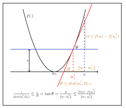
Figure 1: A geometric illustration of the inequality (13), where $dist(w^{\dagger}_{\epsilon},\Omega_{*})=|w^{\dagger}_{\epsilon}-w^{*}_{\epsilon}|$.

Proof  Given any $\mathbf{u}\in\mathcal{L}_{\epsilon}$, let $\mathbf{g}_{\mathbf{u}}$ be any subgradient in $\partial f(\mathbf{u})$ and $\mathbf{v}_{\mathbf{u}}$ be any vector in $\mathcal{N}_{\Omega}(\mathbf{u})$. By the convexity of $f(\cdot)$ and the definition of normal cone, we have

$$f(\mathbf{u}^{*})-f(\mathbf{u})\geq(\mathbf{u}^{*}-\mathbf{u})^{\top}\mathbf{g}_{\mathbf{u}}\geq(\mathbf{u}^{*}-\mathbf{u})^{\top}\left(\mathbf{g}_{\mathbf{u}}+\mathbf{v}_{\mathbf{u}}\right),$$

where $\mathbf{u}^{*}$ is the closest point in $\Omega_{*}$ to $\mathbf{u}$. This inequality further implies

$$\|\mathbf{u}^{*}-\mathbf{u}\|_{2} \|\mathbf{g}_{\mathbf{u}}+\mathbf{v}_{\mathbf{u}}\|_{2}\geq f(\mathbf{u})-f(\mathbf{u}^{*})=\epsilon,\quad\forall\mathbf{g}_{\mathbf{u}}\in\partial f(\mathbf{u})\text{ and }\mathbf{v}_{\mathbf{u}}\in\mathcal{N}_{\Omega}(\mathbf{u})$$ (14)

where the equality is because $\mathbf{u}\in\mathcal{L}_{\epsilon}$. By (14) and the definition of $B_{\epsilon}$, we obtain

$$B_{\epsilon}\|\mathbf{g}_{\mathbf{u}}+\mathbf{v}_{\mathbf{u}}\|_{2}\geq\epsilon\Longrightarrow\|\mathbf{g}_{\mathbf{u}}+\mathbf{v}_{\mathbf{u}}\|_{2}\geq\epsilon/B_{\epsilon}.$$

Since $\mathbf{g}_{\mathbf{u}}+\mathbf{v}_{\mathbf{u}}$ can be any element in $\partial f(\mathbf{u})+\mathcal{N}_{\Omega}(\mathbf{u})$, we have $\rho_{\epsilon}\geq\frac{\epsilon}{B_{\epsilon}}$ by the definition (6).

To prove (13), we assume $\mathbf{w}\in\Omega\backslash\mathcal{S}_{\epsilon}$ and thus $\mathbf{w}^{\dagger}_{\epsilon}\in\mathcal{L}_{\epsilon}$; otherwise it is trivial. In the proof of Lemma 1, we have shown that (see (9)) there exists $\mathbf{g}\in\partial f(\mathbf{w}_{\epsilon}^{\dagger})$ and $\mathbf{v}\in\mathcal{N}_{\Omega}(\mathbf{w}^{\dagger}_{\epsilon})$ such that $f(\mathbf{w})-f(\mathbf{w}^{\dagger}_{\epsilon})\geq\|\mathbf{w}-\mathbf{w}^{\dagger}_{\epsilon}\|_{2}\|\mathbf{g}+\mathbf{v}/\zeta\|_{2}$, which, according to (14) with $\mathbf{u}=\mathbf{w}^{\dagger}_{\epsilon}$, $\mathbf{g}_{\mathbf{u}}=\mathbf{g}$ and $\mathbf{v}_{\mathbf{u}}=\mathbf{v}/\zeta$, leads to (13).  
A geometric explanation of the inequality (13) in one dimension is shown in Figure 1. With Lemma 4, the iteration complexity of RSG can be stated in terms of $B_{\epsilon}$ in the following corollary of Theorem 3.

Corollary 5

Suppose Assumption 1 holds. The iteration complexity of RSG for obtaining an $2\epsilon$-optimal solution is $O(\frac{\alpha^{2}G^{2}B_{\epsilon}^{2}}{\epsilon^{2}}\lceil\log_{\alpha}(\frac{\epsilon_{0}}{\epsilon})\rceil)$ provided $t=\frac{\alpha^{2}G^{2}B_{\epsilon}^{2}}{\epsilon^{2}}$ and $K=\lceil\log_{\alpha}(\frac{\epsilon_{0}}{\epsilon})\rceil$.

We will compare this result with SG in Section 7. Compared to the standard SG, the above improved result of RSG does require knowing strong knolwedge about $f$. In particular, one issue is that the above improved complexity is obtained by choosing $t=\frac{\alpha^{2}G^{2}B_{\epsilon}^{2}}{\epsilon^{2}}$, which requires knowing the order of magnitude of $B_{\epsilon}$, if not its exact value. To address the issue of unknown $B_{\epsilon}$ for general problems, in the next section, we consider different families of problems that admit a local error bound condition and show that the requirement of knowing $B_{\epsilon}$ is relaxed to knowing some particular parameters related to the local error bound.

5 RSG for Some Classes of Non-smooth Non-strongly Convex Optimization

In this section, we consider a particular family of problems that admit local error bounds and show the improved iteration complexities of RSG compared to standard SG method.

5.1 Complexity for the Problems with Local Error Bounds

We first define local error bound of the objective function.

Definition 6

We say $f(\cdot)$ admits a local error bound on the $\epsilon$-sublevel set $\mathcal{S}_{\epsilon}$ if

$$\|\mathbf{w}-\mathbf{w}^{*}\|_{2}\leq c(f(\mathbf{w})-f_{*})^{\theta},\quad\forall\mathbf{w}\in\mathcal{S}_{\epsilon},$$ (15)

where $\mathbf{w}^{*}$ is the closet point in $\Omega_{*}$ to $\mathbf{w}$, $\theta\in(0,1]$ and $0<c<\infty$ are constants.

Because $\mathcal{S}_{\epsilon_{2}}\subset\mathcal{S}_{\epsilon_{1}}$ for $\epsilon_{2}\leq\epsilon_{1}$, if (15) holds for some $\epsilon$, it will always hold when $\epsilon$ decreases to zero with the same $\theta$ and $c$. Indeed, a smaller $\epsilon$ may induce a smaller value of $c$. It is notable that the local error bound condition has been extensively studied in the community of optimization, mathematical programming and variational analysis (Yang, 2009; Li, 2010, 2013; Artacho and Geoffroy, 2008; Kruger, 2015; Drusvyatskiy et al., 2014; Li and Mordukhovich, 2012; Hou et al., 2013; Zhou and So, 2017; Zhou et al., 2015), to name just a few of them. The value of $\theta$ has been exhibited for many problems. For certain problems, the value of $c$ is also computable (c.f. examples in Bolte et al. (2017)).

If the problem admits a local error bound like (15), RSG can achieve a better iteration complexity than $O(1/\epsilon^{2})$. In particular, the property (15) implies

$$B_{\epsilon}\leq c\epsilon^{\theta}.$$ (16)

Replacing $B_{\epsilon}$ in Corollary 5 by this upper bound and choosing $t=\frac{\alpha^{2}G^{2}c^{2}}{\epsilon^{2(1-\theta)}}$ in RSG if $c$ and $\theta$ are known, we obtain the following complexity of RSG.

Corollary 7

Suppose Assumption 1 holds and $f(\cdot)$ admits a local error bound on $\mathcal{S}_{\epsilon}$. The iteration complexity of RSG for obtaining an $2\epsilon$-optimal solution is $O\left(\frac{\alpha^{2}G^{2}c^{2}}{\epsilon^{2(1-\theta)}}\log_{\alpha}\left(\frac{\epsilon_{0}}{\epsilon}\right)\right)$ provided $t=\frac{\alpha^{2}G^{2}c^{2}}{\epsilon^{2(1-\theta)}}$ and $K=\lceil\log_{\alpha}(\frac{\epsilon_{0}}{\epsilon})\rceil$.

Remark: If $t=\Theta(\frac{\alpha^{2}G^{2}}{\epsilon^{2(1-\theta)}})>\frac{\alpha^{2}G^{2}c^{2}}{\epsilon^{2(1-\theta)}}$, then the same order of iteration complexity remains. If one aims to find a point $\mathbf{w}$ such that $\|\mathbf{w}-\mathbf{w}^{*}\|_{2}\leq\epsilon$, we can apply RSG to find a solution $\mathbf{w}$ such that $f(\mathbf{w})-f_{*}\leq(\epsilon/c)^{1/\theta}\leq\epsilon$ (where the last inequality is due to $\theta\leq 1$ and assuming $c\geq 1$ without loss of generality). Then under the local error bound condition, we have $\|\mathbf{w}-\mathbf{w}^{*}\|_{2}\leq c(f(\mathbf{w})-f_{*})^{\theta}\leq\epsilon$. For finding a solution $\mathbf{w}$ such that $f(\mathbf{w})-f_{*}\leq(\epsilon/c)^{1/\theta}\leq\epsilon$, RSG requires an iteration complexity of $\widetilde{O}(\frac{1}{\epsilon^{2(1-\theta)/\theta}})$. Therefore, in order to find a solution $\mathbf{w}$ such that $\|\mathbf{w}-\mathbf{w}^{*}\|_{2}\leq\epsilon$, the iteration complexity of RSG is $\widetilde{O}(\frac{1}{\epsilon^{2(1-\theta)/\theta}})$.

Next, we will consider different convex optimization problems that admit a local error bound on $\mathcal{S}_{\epsilon}$ with different $\theta$ and show the faster convergence of RSG when applied to these problems.

5.2 Linear Convergence for Polyhedral Convex Optimization

In this subsection, we consider a special family of non-smooth and non-strongly convex problems where the epigraph of $f(\cdot)$ over $\Omega$ is a polyhedron. In this case, we call (1) a polyhedral convex minimization problem. We show that, in polyhedral convex minimization problem, $f(\cdot)$ has a linear growth property and admits a local error bound with $\theta=1$ so that $B_{\epsilon}\leq c\epsilon$ for a constant $c<\infty$.

Lemma 8 (Polyhedral Error Bound Condition)

Suppose $\Omega$ is a polyhedron and the epigraph of $f(\cdot)$ is also polyhedron. There exists a constant $\kappa>0$ such that

$$\|\mathbf{w}-\mathbf{w}^{*}\|_{2}\leq\frac{f(\mathbf{w})-f_{*}}{\kappa},\quad\forall\mathbf{w}\in\Omega.$$

Thus, $f(\cdot)$ admits a local error bound on $\mathcal{S}_{\epsilon}$ with $\theta=1$ and $c=\frac{1}{\kappa}$  (so $B_{\epsilon}\leq\frac{\epsilon}{\kappa}$) for any $\epsilon>0$.

Remark: The above inequality is also known as weak sharp minimum condition in literature (Burke and Ferris., 1993; Studniarski and Ward, 1999; Ferris, 1991; Burke and Deng, 2002, 2005, 2009). A proof of Lemma 8 is given by Burke and Ferris. (1993). We also provide a proof in (Yang and Lin, 2016). We remark that the above result can be extended to any valid norm to measure the distance between $\mathbf{w}$ and $\mathbf{w}_{*}$. Lemma 8 generalizes Lemma 4 in (Gilpin et al., 2012), which requires $\Omega$ to be a bounded polyhedron, to a similar result where $\Omega$ can be an unbounded polyhedron. This generalization is simple but useful because it helps the development of efficient algorithms based on this error bound for unconstrained problems without artificially including a box constraint.

Lemma 8 provides the basis for RSG to achieve a linear convergence for the polyhedral convex minimization problems. In fact, the following linear convergence of RSG can be obtained if we plugin the values of $\theta=1$ and $c=\frac{1}{\kappa}$ into Corollary 7.

Corollary 9

Suppose Assumption 1 holds and (1) is a polyhedral convex minimization problem. The iteration complexity of RSG for obtaining an $\epsilon$-optimal solution is $O(\frac{\alpha^{2}G^{2}}{\kappa^{2}}\lceil\log_{\alpha}(\frac{\epsilon_{0}}{\epsilon})\rceil)$ provided $t=\frac{\alpha^{2}G^{2}}{\kappa^{2}}$ and $K=\lceil\log_{\alpha}(\frac{\epsilon_{0}}{\epsilon})\rceil$.

We want to point out that Corollary 9 can be proved directly by replacing $\mathbf{w}^{\dagger}_{k-1,\epsilon}$ by $\mathbf{w}^{*}_{k-1}$ and replacing $\rho_{\epsilon}$ by $\kappa$ in the proof of Theorem 3. Here, we derive it as a corollary of a more general result. We also want to mention that, as shown by Renegar (2015), the linear convergence rate in Corollary 9 can be also obtained by a SG method for the historically best solution, provided $f_{*}$ is known.

Examples.

Many non-smooth and non-strongly convex machine learning problems satisfy the assumptions of Corollary 9, for example, $\ell_{1}$ or $\ell_{\infty}$ constrained or regularized piecewise linear loss minimization. In many machine learning tasks (e.g., classification and regression), there exists a set of data $\{(\mathbf{x}_{i},y_{i})\}_{i=1,2,\dots,n}$ and one often needs to solve the following empirical risk minimization problem

$$\min_{\mathbf{w}\in\mathbb{R}^{d}}f(\mathbf{w})\triangleq\frac{1}{n}\sum_{i=1}^{n}\ell(\mathbf{w}^{\top}\mathbf{x}_{i},y_{i})+R(\mathbf{w}),$$

where $R(\mathbf{w})$ is a regularization term and $\ell(z,y)$ denotes a loss function. We consider a special case where (a) $R(\mathbf{w})$ is a $\ell_{1}$ regularizer, $\ell_{\infty}$ regularizer or an indicator function of a $\ell_{1}$/$\ell_{\infty}$ ball centered at zero; and (b) $\ell(z,y)$ is any piecewise linear loss function, including hinge loss $\ell(z,y)=\max(0,1-yz)$, absolute loss $\ell(z,y)=|z-y|$, $\epsilon$-insensitive loss $\ell(z,y)=\max(|z-y|-\epsilon,0)$, and etc (Yang et al., 2014). It is easy to show that the epigraph of $f(\mathbf{w})$ is a polyhedron if $f(\mathbf{w})$ is defined as a sum of any of these regularization terms and any of these loss functions. In fact, a piecewise linear loss functions can be generally written as

$$\ell(\mathbf{w}^{\top}\mathbf{x},y)=\max_{1\leq j\leq m}a_{j}\mathbf{w}^{\top}\mathbf{x}+b_{j},$$ (17)

where $(a_{j},b_{j})$ for $j=1,2,\dots,m$ are finitely many pairs of scalars. The formulation (17) indicates that $\ell(\mathbf{w}^{\top}\mathbf{x},y)$ is a piecewise affine function so that its epigraph is a polyhedron. In addition, the $\ell_{1}$ or $\ell_{\infty}$ norm is also a polyhedral function because we can represent them as

$$\|\mathbf{w}\|_{1}=\sum_{i=1}^{d}\max(w_{i},-w_{i}),\quad\|\mathbf{w}\|_{\infty}=\max_{1\leq i\leq d}|w_{i}|=\max_{1\leq i\leq d}\max(w_{i},-w_{i}).$$

Since the sum of finitely many polyhedral functions is also a polyhedral function, the epigraph of $f(\mathbf{w})$ is a polyhedron.

Another important family of problems whose objective function has a polyhedral epigraph is submodular function minimization. Let $V=\{1,\ldots,d\}$ be a set and $2^{V}$ denote its power set. A submodular function $F(A):2^{V}\rightarrow\mathbb{R}$ is a set function such that $F(A)+F(B)\geq F(A\cup B)+F(A\cap B)$ for all subsets $A,B\subseteq V$ and $F(\emptyset)=0$. A submodular function minimization can be cast into a non-smooth convex optimization using the Lovász extension (Bach, 2013). In particular, let the base polyhedron $B(F)$ be defined as

$$B(F)=\{\mathbf{s}\in\mathbb{R}^{d},\mathbf{s}(V)=F(V),\forall A\subseteq V,\mathbf{s}(A)\leq F(A)\},$$

where $\mathbf{s}(A)=\sum_{i\in A}s_{i}$. Then the Lovász extension of $F(A)$ is $f(\mathbf{w})=\max_{\mathbf{s}\in B(F)}\mathbf{w}^{\top}\mathbf{s}$, and $\min_{A\subseteq V}F(A)=\min_{\mathbf{w}\in[0,1]^{d}}f(\mathbf{w})$. As a result, a submodular function minimization is essentially a non-smooth and non-strongly convex optimization with a polyhedral epigraph.

5.3 Improved Convergence for Locally Semi-Strongly Convex Problems

First, we give a definition of local semi-strong convexity.

Definition 10

A function $f(\mathbf{w})$ is semi-strongly convex on the $\epsilon$-sublevel set $\mathcal{S}_{\epsilon}$ if there exists $\lambda>0$ such that

$$\frac{\lambda}{2}\|\mathbf{w}-\mathbf{w}^{*}\|_{2}^{2}\leq f(\mathbf{w})-f(\mathbf{w}^{*}),\quad\forall\mathbf{w}\in\mathcal{S}_{\epsilon}$$ (18)

where $\mathbf{w}^{*}$ is the closest point to $\mathbf{w}$ in the optimal set.

We refer to the property (18) as local semi-strong convexity when $\mathcal{S}_{\epsilon}\neq\Omega$. The two papers (Gong and Ye, 2014; Necoara et al., 2015) have explored the semi-strong convexity on the whole domain $\Omega$ to prove linear convergence of smooth optimization problems. In (Necoara et al., 2015), the inequality (18) is also called second-order growth property. They have also shown that a class of problems satisfy (18) (see examples given below). The inequality (18) indicates that $f(\cdot)$ admits a local error bound on $\mathcal{S}_{\epsilon}$ with $\theta=\frac{1}{2}$ and $c=\sqrt{\frac{2}{\lambda}}$, which leads to the following the corollary about the iteration complexity of RSG for locally semi-strongly convex problems.

Corollary 11

Suppose Assumption 1 holds and $f(\mathbf{w})$ is semi-strongly convex on $\mathcal{S}_{\epsilon}$. Then $B_{\epsilon}\leq\sqrt{\frac{2\epsilon}{\lambda}}$ and the iteration complexity of RSG for obtaining an $2\epsilon$-optimal solution is $O(\frac{2\alpha^{2}G^{2}}{\lambda\epsilon}\lceil\log_{\alpha}(\frac{\epsilon_{0}}{\epsilon})\rceil)$ provided $t=\frac{2\alpha^{2}G^{2}}{\lambda\epsilon}$ and $K=\lceil\log_{\alpha}(\frac{\epsilon_{0}}{\epsilon})\rceil$.

Remark: Here, we obtain an $\widetilde{O}(1/\epsilon)$ iteration complexity ($\widetilde{O}(\cdot)$ suppresses constants and logarithmic terms) only with local semi-strong convexity. It is obvious that strong convexity implies local semi-strong convexity (Hazan and Kale, 2011) but not vice versa.

Examples

Consider a family of functions in the form of $f(\mathbf{w})=h(X\mathbf{w})+r(\mathbf{w})$, where $X\in\mathbb{R}^{n\times d}$, $h(\cdot)$ is strongly convex on any compact set and $r(\cdot)$ has a polyhedral epigraph. According to (Gong and Ye, 2014; Necoara et al., 2015), such a function $f(\mathbf{w})$ satisfies (18) for any $\epsilon\leq\epsilon_{0}$ with a constant value for $\lambda$. Although smoothness is assumed for $h(\cdot)$ in (Gong and Ye, 2014; Necoara et al., 2015), we find that it is not necessary for proving (18). We state this result as the lemma below.

Lemma 12

Suppose Assumption 1 holds, $\Omega=\{\mathbf{w}\in\mathbb{R}^{d}|C\mathbf{w}\leq\mathbf{b}\}$ with $C\in\mathbb{R}^{k\times d}$ and $\mathbf{b}\in\mathbb{R}^{k}$, and $f(\mathbf{w})=h(X\mathbf{w})+r(\mathbf{w})$ where $h:\mathbb{R}^{n}\rightarrow\mathbb{R}$ satisfies $\text{dom}(h)=\mathbb{R}^{k}$ and is a strongly convex function on any compact set in $\mathbb{R}^{n}$, and $r(\mathbf{w})$ has a polyhedral epigraph. Then, $f(w)$ satisfies (18) for any $\epsilon\leq\epsilon_{0}$.

The proof of this lemma can be found in (Gong and Ye, 2014; Necoara et al., 2015; Necoara and Clipici, 2016). For example, it is almost identical to the proof of Lemma 1 in (Gong and Ye, 2014) which assumes $h(\cdot)$ is smooth). However, a similar result holds without the smoothness of $h(\cdot)$.

The function of this type covers some commonly used loss functions and regularization terms in machine learning and statistics. For example, we can consider robust regression with/without $\ell_{1}$ regularizer (Xu et al., 2010; Bertsimas and Copenhaver, 2014):

$$\min_{\mathbf{w}\in\Omega}\frac{1}{n}\sum\limits_{i=1}^{n}|\mathbf{x}_{i}^{\top}\mathbf{w}-y_{i}|^{p}+\lambda\|\mathbf{w}\|_{1},$$ (19)

where $p\in(1,2)$, $\mathbf{x}_{i}\in\mathbb{R}^{d}$ denotes the feature vector and $y_{i}$ is the target output. The objective function is in the form of $h(X\mathbf{w})+r(\mathbf{w})$ where $X$ is a $n\times d$ matrix with $\mathbf{x}_{1},\mathbf{x}_{2},\dots,\mathbf{x}_{n}$ being its rows and $h(\mathbf{u}):=\sum_{i=1}^{n}|u_{i}-y_{i}|^{p}$. According to (Goebel and Rockafellar, 2007), $h(\mathbf{u})$ is a strongly convex function on any compact set so that the objective function above is semi-strongly convex on $\mathcal{S}_{\epsilon}$ for any $\epsilon\leq\epsilon_{0}$.

5.4 Improved Convergence for Convex Problems with KL property

Lastly, we consider a family of non-smooth functions with a local Kurdyka-Łojasiewicz (KL) property. The definition of KL property is given below.

Definition 13

The function $f(\mathbf{w})$ has the Kurdyka - Łojasiewicz (KL) property at $\bar{\mathbf{w}}$ if there exist $\eta\in(0,\infty]$, a neighborhood $U_{\bar{\mathbf{w}}}$ of $\bar{\mathbf{w}}$ and a continuous concave function $\varphi:[0,\eta)\rightarrow\mathbb{R}_{+}$ such that (i) $\varphi(0)=0$; (ii) $\varphi$ is continuous on $(0,\eta)$; (iii) for all $s\in(0,\eta)$, $\varphi^{\prime}(s)>0$; (iv) and for all $\mathbf{w}\in U_{\bar{\mathbf{w}}}\cap\{\mathbf{w}:f(\bar{\mathbf{w}})<f(\mathbf{w})<f(\bar{\mathbf{w}})+\eta\}$, the Kurdyka - Łojasiewicz (KL) inequality holds

$$\varphi^{\prime}(f(\mathbf{w})-f(\bar{\mathbf{w}}))\|\partial f(\mathbf{w})\|_{2}\geq 1,$$ (20)

where $\|\partial f(\mathbf{w})\|_{2}:=\min_{\mathbf{g}\in\partial f(\mathbf{w})}\|\mathbf{g}\|_{2}$.

The function $\varphi$ is called the desingularizing function of $f$ at $\bar{\mathbf{w}}$, which sharpens the function $f(\mathbf{w})$ by reparameterization. An important desingularizing function is in the form of $\varphi(s)=cs^{1-\beta}$ for some $c>0$ and $\beta\in[0,1)$, by which, (20) gives the KL inequality

$$\|\partial f(\mathbf{w})\|_{2}\geq\frac{1}{c(1-\beta)}(f(\mathbf{w})-f(\bar{\mathbf{w}}))^{\beta}.$$

Note that all semi-algebraic functions satisfy the KL property at any point (Bolte et al., 2014). Indeed, all the concrete examples given before satisfy the Kurdyka - Łojasiewicz property. For more discussions about the KL property, we refer readers to (Bolte et al., 2014, 2007; Schneider and Uschmajew, 2015; Attouch et al., 2013; Bolte et al., 2006). The following corollary states the iteration complexity of RSG for unconstrained problems that have the KL property at each $\bar{\mathbf{w}}\in\Omega_{*}$ .

Corollary 14

Suppose Assumption 1 holds, $f(\mathbf{w})$ satisfies a (uniform) Kurdyka - Łojasiewicz property at any $\bar{\mathbf{w}}\in\Omega_{*}$ with the same desingularizing function $\varphi$ and constant $\eta$, and

$$\mathcal{S}_{\epsilon}\subset\cup_{\bar{\mathbf{w}}\in\Omega_{*}}\left[U_{\bar{\mathbf{w}}}\cap\{\mathbf{w}:f(\bar{\mathbf{w}})<f(\mathbf{w})<f(\bar{\mathbf{w}})+\eta\}\right].$$ (21)

RSG has an iteration complexity of $O\left(\alpha^{2}G^{2}(\frac{\varphi(\epsilon)}{\epsilon})^{2}\lceil\log_{\alpha}(\frac{\epsilon_{0}}{\epsilon})\rceil\right)$ for obtaining an $2\epsilon$-optimal solution provided $t=\alpha^{2}G^{2}(\varphi(\epsilon)/\epsilon)^{2}$. In addition, if $\varphi(s)=cs^{1-\beta}$ for some $c>0$ and $\beta\in[0,1)$, the iteration complexity of RSG is $O(\frac{\alpha^{2}G^{2}c^{2}(1-\beta)^{2}}{\epsilon^{2\beta}}\lceil\log_{\alpha}(\frac{\epsilon_{0}}{\epsilon})\rceil)$ provided $t=\frac{\alpha^{2}G^{2}c^{2}}{\epsilon^{2\beta}}$ and $K=\lceil\log_{\alpha}(\frac{\epsilon_{0}}{\epsilon})\rceil$.

Proof  We can prove the above corollary following a result in (Bolte et al., 2017) as presented in Proposition 1 in the appendix. According to Proposition 1, if $f(\cdot)$ satisfies the KL property at $\bar{\mathbf{w}}$, then for all $\mathbf{w}\in U_{\bar{\mathbf{w}}}\cap\{\mathbf{w}:f(\bar{\mathbf{w}})<f(\mathbf{w})<f(\bar{\mathbf{w}})+\eta\}$ it holds that $\|\mathbf{w}-\mathbf{w}^{*}\|_{2}\leq\varphi(f(\mathbf{w})-f(\bar{\mathbf{w}}))$. It then, under the uniform condition in (21), implies that, for any $\mathbf{w}\in\mathcal{S}_{\epsilon}$

$$\|\mathbf{w}-\mathbf{w}^{*}\|_{2}\leq\varphi(f(\mathbf{w})-f_{*})\leq\varphi(\epsilon),$$

where we use the monotonic property of $\varphi$. Then the first conclusion follows similarly as Corollary 5 by noting $B_{\epsilon}\leq\varphi(\epsilon)$. The second conclusion immediately follows by setting $\varphi(s)=cs^{1-\beta}$ in the first conclusion. Please note that the above inequality implies the local error bound condition with $\theta=1-\beta$ for $\varphi(s)=cs^{1-\beta}$.  

While the conclusion in Corollary 14 hinges on a condition in (21), in practice many convex functions (e.g., continuous semi-algebraic or subanalytic functions) satisfy the KL property with $U=\mathbb{R}^{d}$ and any finite $\eta<\infty$ (Attouch et al., 2010; Bolte et al., 2017; Li, 2010).

It is worth mentioning that to our best knowledge, the present work is the first to leverage the KL property for developing improved subgradient methods, though it has been explored in non-convex and convex optimization for deterministic descent methods for smooth optimization (Bolte et al., 2017, 2014; Attouch et al., 2010; Karimi et al., 2016). For example, Bolte et al. (2017) studied the convergence of subgradient descent sequence for minimizing a convex function under an error bound condition. A sequence $\{\mathbf{x}_{k}\}$ is called a subgradient descent sequence if there exist $a>0,b>0$ it satisfies two conditions, namely sufficient decrease condition $f(\mathbf{x}_{k})+a\|\mathbf{x}_{k}-\mathbf{x}_{k-1}\|_{2}^{2}\leq f(\mathbf{x}_{k-1})$, and relative error condition, i.e., there exists $\omega_{k}\in\partial f(\mathbf{x}_{k})$ such that $\|\omega_{k}\|_{2}\leq b\|\mathbf{x}_{k}-\mathbf{x}_{k-1}\|_{2}$. However, for a general non-smooth function $f(\mathbf{x})$, the sequence generated by subgradient method, i.e., $\mathbf{x}_{k}=\mathbf{x}_{k-1}-\eta_{k}\partial\nabla f(\mathbf{x}_{k-1})$ do not necessarily satisfy the above two conditions. Instead, Bolte et al. (2017) considered proximal gradient method that only applies to a smaller family of functions consisting of a smooth component and a non-smooth component by assuming the proximal mapping for the non-smooth component can be efficiently computed. In contrast, our algorithm and analysis are developed for much general non-smooth functions.

6 Variants of RSG without knowing the constant $c$ and the exponent $\theta$ in the local error bound

In Section 5, we have discussed the local error bound and presented several classes of problems to reveal the magnitude of $B_{\epsilon}$, i.e., $B_{\epsilon}=c\epsilon^{\theta}$. For some problems, the value of $\theta$ is exhibited. However, the value of the constant $c$ could be still difficult to estimate, which renders it challenging to set the appropriate value $t=\frac{\alpha^{2}c^{2}G^{2}}{\epsilon^{2(1-\theta)}}$ for inner iterations of RSG. In practice, one might use a sufficiently large $c$ to set up the value of $t$. However, such an approach might be vulnerable to both over-estimation and under-estimation of $t$. Over-estimating the value of $t$ leads to a waste of iterations while under-estimation leads to an less accurate solution that might not reach to the target accuracy level. In addition, for some problems the value of $\theta$ is still an open problem. One interesting family of objective functions in machine learning is the sum of piecewise linear loss over training data and a nuclear norm regularizer or an overlapped or non-overlapped group lasso regularizer. In this section, we present variants of RSG that can be implemented without knowing the value of $c$ in the local error bound condition and even the value of exponent $\theta$, and prove their improved convergence over the SG method.

6.1 RSG without knowing $c$

The key idea is to use an increasing sequence of $t$ and another level of restarting for RSG. The detailed steps are presented in Algorithm 3, to which we refer as R²SG. With large enough $t_{1}$ in R²SG, the complexity of R²SG for finding an $\epsilon$ solution is given by the theorem below.

Theorem 15

Suppose $\epsilon\leq\epsilon_{0}/4$ and $K=\lceil\log_{\alpha}(\epsilon_{0}/\epsilon)\rceil$. Let $t_{1}$ in Algorithm 3 be large enough so that there exists $\hat{\epsilon}_{1}\in(\epsilon,\epsilon_{0}/2)$, with which $f(\cdot)$ satisfies a local error bound condition on $\mathcal{S}_{\hat{\epsilon}_{1}}$ with $\theta\in(0,1)$ and the constant $\hat{c}$, and $t_{1}=\frac{\alpha^{2}\hat{c}^{2}G^{2}}{\hat{\epsilon}_{1}^{2(1-\theta)}}$. Then, with at most $S=\lceil\log_{2}(\hat{\epsilon}_{1}/\epsilon)\rceil+1$ calls of RSG in Algorithm 3, we find a solution $\mathbf{w}^{S}$ such that $f(\mathbf{w}^{S})-f_{*}\leq 2\epsilon$. The total number of iterations of R²SG for obtaining $2\epsilon$-optimal solution is upper bounded by $T_{S}=O\left(\frac{\hat{c}^{2}G^{2}}{\epsilon^{2(1-\theta)}}\lceil\log_{\alpha}(\frac{\epsilon_{0}}{\epsilon})\rceil\right)$.

Proof  Since $K=\lceil\log_{\alpha}(\epsilon_{0}/\epsilon)\rceil\geq\lceil\log_{\alpha}(\epsilon_{0}/\hat{\epsilon}_{1})\rceil$ and $t_{1}=\frac{\alpha^{2}\hat{c}^{2}G^{2}}{\hat{\epsilon}_{1}^{2(1-\theta)}}$, we can apply Corollary 7 with $\epsilon=\hat{\epsilon}_{1}$ to the first call of RSG in Algorithm 3 so that the output $\mathbf{w}^{1}$ satisfies

$$f(\mathbf{w}^{1})-f_{*}\leq 2\hat{\epsilon}_{1}.$$ (22)

Then, we consider the second call of RSG with the initial solution $\mathbf{w}^{1}$ satisfying (22). By the setup $K=\lceil\log_{\alpha}(\epsilon_{0}/\epsilon)\rceil\geq\lceil\log_{\alpha}(2\hat{\epsilon}_{1}/(\hat{\epsilon}_{1}/2))\rceil$ and $t_{2}=t_{1}2^{2(1-\theta)}=\frac{\hat{c}^{2}G^{2}}{(\hat{\epsilon}_{1}/2)^{2(1-\theta)}}$, we can apply Corollary 7 with $\epsilon=\hat{\epsilon}_{1}/2$ and $\epsilon_{0}=2\hat{\epsilon}_{1}$ so that the output $\mathbf{w}^{2}$ of the second call satisfies $f(\mathbf{w}^{2})-f_{*}\leq\hat{\epsilon}_{1}$. By repeating this argument for all the subsequent calls of RSG, with at most $S=\lceil\log_{2}(\hat{\epsilon}_{1}/\epsilon)\rceil+1$ calls, Algorithm 3 ensures that

$$f(\mathbf{w}^{S})-f_{*}\leq 2\hat{\epsilon}_{1}/2^{S-1}\leq 2\epsilon$$

The total number of iterations during the $S$ calls of RSG is bounded by

$$T_{S} =K\sum_{s=1}^{S}t_{s}=K\sum_{s=1}^{S}t_{1}2^{2(s-1)(1-\theta)}=Kt_{1}2^{2(S-1)(1-\theta)}\sum_{s=1}^{S}\left(\frac{1}{2^{2(1-\theta)}}\right)^{S-s}$$

$$\leq\frac{Kt_{1}2^{2(S-1)(1-\theta)}}{1-1/2^{2(1-\theta)}}\leq O\left(Kt_{1}\left(\frac{\hat{\epsilon}_{1}}{\epsilon}\right)^{2(1-\theta)}\right)=O\left(\frac{\hat{c}^{2}G^{2}}{\epsilon^{2(1-\theta)}}\lceil\log_{\alpha}(\frac{\epsilon_{0}}{\epsilon})\rceil\right).$$

 

Algorithm 3 RSG with restarting: R²SG

1:  Input: the number of iterations $t_{1}$ in each stage of the first call of RSG and the number of stages $K$ in each call of RSG

2:  Initialization: $\mathbf{w}^{0}\in\Omega$;

3:  for $s=1,2\ldots,S$ do

4:     Let $\mathbf{w}^{s}=\text{RSG}(\mathbf{w}^{s-1},K,t_{s},\alpha)$

5:     Let $t_{s+1}=t_{s}2^{2(1-\theta)}$

6:  end for

Remark: We make several remarks about Algorithm 3 and Theorem 15: (i) Theorem 15 applies only when $\theta\in(0,1)$. If $\theta=1$, in order to have an increasing sequence of $t_{s}$, we can set $\theta$ in Algorithm 3 to a little smaller value than $1$ in practical implementation, and the iteration complexity in Theorem 15 implies that R²SG can enjoy a convergence rate close to linear convergence for problems satisfying the weak sharp minimum condition. (ii) the $\epsilon_{0}$ in the implementation of RSG (Algorthm 2) can be re-calibrated for $s\geq 2$ to improve the performance (e.g., one can use the relationship $f(\mathbf{w}_{s-1})-f_{*}=f(\mathbf{w}_{s-2})-f_{*}+f(\mathbf{w}_{s-1})-f(\mathbf{w}_{s-2})$ to do re-calibration); (iii) as a tradeoff, the exiting criterion of R²SG is not as automatic as RSG. In fact, the total number of calls $S$ of RSG for obtaining an $2\epsilon$-optimal solution depends on an unknown parameter (namely $\hat{\epsilon}_{1}$). In practice, one could use other stopping criteria to terminate the algorithm. For example, in machine learning applications one can monitor the performance on the validation data set to terminate the algorithm. (vi) The quantities $\hat{\epsilon}_{1}$, $S$ in the proof above are implicitly determined by $t_{1}$ and one does not need to compute $\hat{\epsilon}_{1}$ and $S$ in order to apply Algorithm 3. Finally, we note that when a local strong convexity condition holds on $\mathcal{S}_{\hat{\epsilon}_{1}}$ with $\hat{\epsilon}_{1}\geq\epsilon$ one might derive an iteration complexity of $O(1/\epsilon)$ for SG by first showing that SG converges to $\mathcal{S}_{\hat{\epsilon}_{1}}$ with a number of iterations independent of $\epsilon$, then showing that the iterates stay within $\mathcal{S}_{\hat{\epsilon}_{1}}$ and converge to an $\epsilon$-level set with an iteration complexity of $O(1/\epsilon)$ following existing analysis of SG for strongly convex functions (e.g., Lacoste-Julien et al. (2012)). However, it still needs to know the value of the local strong convexity parameter unlike our result in Theorem 15 that does not need to known the local strong convexity parameter.

6.2 RSG for unknown $\theta$ and $c$

Without knowing $\theta\in(0,1]$ and $c$ to get a sharper local error bound, we can simply let $\theta=0$ and $c=B_{\epsilon^{\prime}}$ with $\epsilon^{\prime}\geq\epsilon$, which still render the inequaity (15) hold (c.f. Definition 6). Then we can employ the same trick to increase the values of $t$. In particular, we start with a sufficiently large value of $t$ and run RSG with $K=\lceil\log_{\alpha}(\epsilon_{0}/\epsilon)\rceil$ stages, and then increase the value of $t$ by a factor of $4$ and repeat the process.

Theorem 16

Let $\theta=0$ in Algorithm 3 and suppose $\epsilon\leq\epsilon_{0}/4$ and $K=\lceil\log_{\alpha}(\epsilon_{0}/\epsilon)\rceil$. Assume $t_{1}$ in Algorithm 3 is large enough so that there exists $\hat{\epsilon}_{1}\in(\epsilon,\epsilon_{0}/2]$ giving $t_{1}=\frac{\alpha^{2}B_{\hat{\epsilon}_{1}}^{2}G^{2}}{\hat{\epsilon}_{1}^{2}}$. Then, with at most $S=\lceil\log_{2}(\hat{\epsilon}_{1}/\epsilon)\rceil+1$ calls of RSG in Algorithm 3, we find a solution $\mathbf{w}^{S}$ such that $f(\mathbf{w}^{S})-f_{*}\leq 2\epsilon$. The total number of iterations of R²SG for obtaining $2\epsilon$-optimal solution is upper bounded by $T_{S}=O\left(\frac{B_{\hat{\epsilon}_{1}}^{2}G^{2}}{\epsilon^{2}}\lceil\log_{\alpha}(\frac{\epsilon_{0}}{\epsilon})\rceil\right)$.

Remark: Since $B_{\epsilon}/\epsilon$ is a monotonically decreasing function in $\epsilon$ (Xu et al., 2017, Lemma 7), such a $t_{1}$ in Theorem 16 exists. Note that if the problem satisfies a KL property as in Corollary 14 and the value of $\beta$ is unknown, the above theorem still holds.

Proof  The proof is similar to that of Theorem 15 except that we let $c=B_{\hat{\epsilon}_{1}}$ and $\theta=0$. Since $K=\lceil\log_{\alpha}(\epsilon_{0}/\epsilon)\rceil\geq\lceil\log_{\alpha}(\epsilon_{0}/\hat{\epsilon}_{1})\rceil$ and $t_{1}=\frac{\alpha^{2}B_{\hat{\epsilon}_{1}}^{2}G^{2}}{\hat{\epsilon}_{1}^{2}}$, we can apply Corollary 5 with $\epsilon=\hat{\epsilon}_{1}$ to the first call of RSG in Algorithm 3 so that the output $\mathbf{w}^{1}$ satisfies

$$f(\mathbf{w}^{1})-f_{*}\leq 2\hat{\epsilon}_{1}.$$ (23)

Then, we consider the second call of RSG with the initial solution $\mathbf{w}^{1}$ satisfying (23). By the setup $K=\lceil\log_{\alpha}(\epsilon_{0}/\epsilon)\rceil\geq\lceil\log_{\alpha}(2\hat{\epsilon}_{1}/(\hat{\epsilon}_{1}/2))\rceil$ and $t_{2}=t_{1}2^{2}=\frac{B_{\hat{\epsilon}_{1}}^{2}G^{2}}{(\hat{\epsilon}_{1}/2)^{2}}$, we can apply Corollary 5 with $\epsilon=\hat{\epsilon}_{1}/2$ and $\epsilon_{0}=2\hat{\epsilon}_{1}$ (noting that $B_{\hat{\epsilon}_{1}}>B_{\hat{\epsilon}_{1}/2}$) so that the output $\mathbf{w}^{2}$ of the second call satisfies $f(\mathbf{w}^{2})-f_{*}\leq\hat{\epsilon}_{1}$. By repeating this argument for all the subsequent calls of RSG, with at most $S=\lceil\log_{2}(\hat{\epsilon}_{1}/\epsilon)\rceil+1$ calls, Algorithm 3 ensures that

$$f(\mathbf{w}^{S})-f_{*}\leq 2\hat{\epsilon}_{1}/2^{S-1}\leq 2\epsilon.$$

The total number of iterations during the $S$ calls of RSG is bounded by

$$T_{S} =K\sum_{s=1}^{S}t_{s}=K\sum_{s=1}^{S}t_{1}2^{2(s-1)}=Kt_{1}2^{2(S-1)}\sum_{s=1}^{S}\left(\frac{1}{2^{2}}\right)^{S-s}$$

$$\leq\frac{Kt_{1}2^{2(S-1)}}{1-1/2^{2}}\leq O\left(Kt_{1}\left(\frac{\hat{\epsilon}_{1}}{\epsilon}\right)^{2}\right)=O\left(\frac{B_{\hat{\epsilon}_{1}}^{2}G^{2}}{\epsilon^{2}}\lceil\log_{\alpha}(\frac{\epsilon_{0}}{\epsilon})\rceil\right).$$

 

7 Discussions and Comparisons

In this section, we further discuss the obtained results and compare them with existing results.

Comparison with the standard SG

The standard SG’s iteration complexity is known as $O(\frac{G^{2}\|\mathbf{w}_{0}-\mathbf{w}^{*}_{0}\|_{2}^{2}}{\epsilon^{2}})$ for achieving an $2\epsilon$-optimal solution. By assuming $t$ is appropriately set in RSG according to Corollary 5, its iteration complexity is $O(\frac{G^{2}B_{\epsilon}^{2}}{\epsilon^{2}}\log(\epsilon_{0}/\epsilon))$, which depends on $B_{\epsilon}^{2}$ instead of $\|\mathbf{w}_{0}-\mathbf{w}_{0}^{*}\|_{2}^{2}$ and only has a logarithmic dependence on $\epsilon_{0}$, the upper bound of $f(\mathbf{w}_{0})-f_{*}$. When the initial solution is far from the optimal set so that $B_{\epsilon}^{2}\ll\|\mathbf{w}_{0}-\mathbf{w}_{0}^{*}\|_{2}^{2}$, RSG could have a lower worst-case complexity. Even if $t$ is not appropriately set up to be larger than $\alpha^{2}G^{2}B_{\epsilon}^{2}/\epsilon^{2}$, Theorem 16 guarantees that the proposed R²SG could still has a lower iteration complexity than that of SG as long as $t_{1}$ is sufficiently large. In some special cases, e.g., when $f$ satisfies the local error bound condition (15) with $\theta\in(0,1]$, RSG only needs $O\left(\frac{1}{\epsilon^{2(1-\theta)}}\log\left(\frac{1}{\epsilon}\right)\right)$ iterations (see Corollary 7 and Theorem 15), which has a better dependency on $\epsilon$ than the complexity of standard SG method.

Comparison with the SG method in (Freund and Lu, 2017)

Freund and Lu (2017) introduced a similar but different growth condition:

$$\|\mathbf{w}-\mathbf{w}^{*}\|_{2}\leq\mathcal{G}\cdot(f(\mathbf{w})-f_{slb}),\quad\forall\mathbf{w}\in\Omega,$$ (24)

where $f_{slb}$ is a strict lower bound of $f_{*}$, by Freund and Lu (2017). The main differences from our key condition (7) are: the left-hand side is the distance of $\mathbf{w}$ to the optimal set in (24) while it is the distance of $\mathbf{w}$ to the $\epsilon$-sublevel set in (7); the right-hand side is the objective gap with respect to $f_{slb}$ in (24) and it is the objective gap with respect to $f_{*}$ in (7); the growth constant $\mathcal{G}$ in (24) varies with $f_{slb}$ and $\rho_{\epsilon}$ in (7) may depend on $\epsilon$ in general.

Freund and Lu’s SG method has an iteration complexity of $O(G^{2}\mathcal{G}^{2}(\frac{\log H}{\epsilon^{\prime}}+\frac{1}{\epsilon^{\prime 2}}))$ for finding a solution $\hat{\mathbf{w}}$ such that $f(\hat{\mathbf{w}})-f_{*}\leq\epsilon^{\prime}(f_{*}-f_{slb})$, where $f_{slb}$ and $\mathcal{G}$ are defined in (24) and $H=\frac{f(\mathbf{w}_{0})-f_{slb}}{f_{*}-f_{slb}}$. In comparison, our RSG can be better if $f_{*}-f_{slb}$ is large. To see this, we represent the complexity in (Freund and Lu, 2017) in terms of the absolute error $\epsilon$ with $\epsilon=\epsilon^{\prime}(f_{*}-f_{slb})$ and obtain $O(G^{2}\mathcal{G}^{2}(\frac{(f_{*}-f_{slb})\log H}{\epsilon}+\frac{(f_{*}-f_{slb})^{2}}{\epsilon^{2}}))$. If the gap $f_{*}-f_{slb}$ is large, e.g., $O(f(\mathbf{w}_{0})-f_{slb})$, the second term is dominating, which is at least $\Omega(\frac{G^{2}\|\mathbf{w}_{0}-\mathbf{w}^{*}_{0}\|_{2}^{2}}{\epsilon^{2}})$ due to the definition of $\mathcal{G}$ in $\eqref{eqn:FreundCond}$. This complexity has the same order of magnitude as the standard SG method so that RSG can be better due to the reasoning in last paragraph. More generally, the iteration complexity of Freund and Lu’s SG method can be reduced to $O(\frac{G^{2}B^{2}_{f_{*}-f{slb}}}{\epsilon^{2}})$ by choosing the best $\mathcal{G}$ in the proof of Theorem 1.1 in (Freund and Lu, 2017), which depends on $f_{*}-f_{slb}$. In comparison, RSG could have a lower complexity if $f_{*}-f_{slb}$ is larger than $\epsilon$ as in Corollary 5 or $\hat{\epsilon}_{1}$ as in Theorem 15. Our experiments in subsection 8.4 also corroborate this point. In addition, RSG can leverage the local error bound condition to enjoy a lower iteration complexity than $O(1/\epsilon^{2})$.

Comparison with (Juditsky and Nesterov, 2014) for uniformly convex function

Juditsky and Nesterov (2014) considered primal-dual subgradient methods for solving the problem (1) with $f$ being uniformly convex, namely,

$$f(\alpha\mathbf{w}+(1-\alpha)\mathbf{v})\leq\alpha f(\mathbf{w})+(1-\alpha)f(\mathbf{v})-\frac{1}{2}\mu\alpha(1-\alpha)[\alpha^{\rho-1}+(1-\alpha)^{\rho-1}]\|\mathbf{w}-\mathbf{v}\|_{2}^{\rho}$$

for any $\mathbf{w}$ and $\mathbf{v}$ in $\Omega$ and any $\alpha\in[0,1]$, where $\rho\in[2,+\infty]$ and $\mu\geq 0$. In this case, the method by (Juditsky and Nesterov, 2014) has an iteration complexity of $O\left(\frac{G^{2}}{\mu^{2/\rho}\epsilon^{2(\rho-1)/\rho}}\right)$. The uniform convexity of $f$ further implies $f(\mathbf{w})-f_{*}\geq\frac{1}{2}\mu\|\mathbf{w}-\mathbf{w}^{*}\|_{2}^{\rho}$ for any $\mathbf{w}\in\Omega$ so that $f(\cdot)$ admits a local error bound on the $\epsilon$-sublevel set $\mathcal{S}_{\epsilon}$ with $c=\left(\frac{2}{\mu}\right)^{\frac{1}{\rho}}$ and $\theta=\frac{1}{\rho}$. Therefore, our RSG has a complexity of $O\left(\frac{G^{2}}{\mu^{2/\rho}\epsilon^{2(\rho-1)/\rho}}\log(\frac{\epsilon_{0}}{\epsilon})\right)$ according to Corollary 7. Compared to (Juditsky and Nesterov, 2014), our complexity is higher by a logarithmic factor. However, we only require the local error bound property of $f$ that is weaker than uniform convexity and also covers much broader family of functions. Note that the above comparison is fair, since for achieving a target $\epsilon$-optimal solution the algorithms presented in (Juditsky and Nesterov, 2014) do need the knowledge of uniform convexity parameter $\rho$ and the parameter $\mu$. It is worth mentioning that Juditsky and Nesterov (2014) also presented algorithms with a fixed number of iterations $T$ as input that achieve adaptive rates without knowledge of $\rho$ and $\mu$. However, they only considered the case when $\rho>=2$, which correponds to $\theta\leq 1/2$ in our notations, while our methods can be applied also when $\theta>1/2$.

8 Experiments

In this section, we present some experiments to demonstrate the effectiveness of RSG. We first consider several applications in machine learning, in particular regression, classification and matrix completion, and focus on the comparison between RSG and SG. Then we make comparison between RSG with Freund & Lu’s SG variant for solving regression problems. In experiments, all compared algorithms use the same initial solution unless otherwise specified.

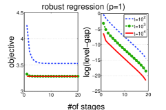
(a) different $t$

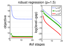
(b) different $t$

(c) different algorithms

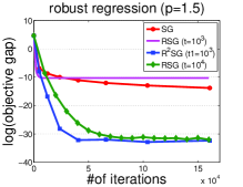
(d) different algorithms

Figure 2: Comparison of RSG with different $t$ and of different algorithms on the housing data. One iteration means one subgradient update in all algorithms. (t1 for R²SG represents the initial value of $t$ in the first call of RSG.)

8.1 Robust Regression

The regression problem is to predict an output $y$ based on a feature vector $\mathbf{x}\in\mathbb{R}^{d}$. Given a set of training examples $(\mathbf{x}_{i},y_{i}),i=1,\ldots,n$, a linear regression model can be found by solving the optimization problem in (19).

We solve two instances of the problem with $p=1$ and $p=1.5$ and $\lambda=0$. We conduct experiments on two data sets from libsvm website , namely housing ($n=506$ and $d=13$) and space-ga ($n=3107$ and $d=6$). We first examine the convergence behavior of RSG with different values for the number of iterations per-stage $t=10^{2}$, $10^{3}$, and $10^{4}$. The value of $\alpha$ is set to $2$ in all experiments. The initial step size of RSG is set to be proportional to $\epsilon_{0}/2$ with the same scaling parameter for different variants. We plot the results on housing data in Figure 2 (a,b) and on space-ga data in Figure 3 (a,b). In each figure, we plot the objective value vs number of stages and the log difference between the objective value and the converged value (to which we refer as level gap). We can clearly see that with different values of $t$ RSG converges to an $\epsilon$-level set and the convergence rate is linear in terms of the number of stages, which is consistent with our theory.

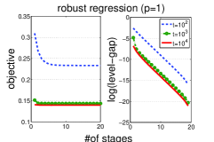
(a) different $t$

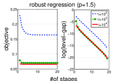
(b) different $t$

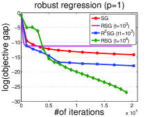
(c) different algorithms

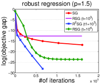
(d) different algorithms

Figure 3: Comparison of RSG with different $t$ and of different algorithms on the space-ga data. One iteration means one subgradient update in all algorithms.

Secondly, we compare with SG to verify the effectiveness of RSG. The baseline SG is implemented with a decreasing step size proportional to $1/\sqrt{\tau}$, where $\tau$ is the iteration index. The initial step size of SG is tuned in a wide range to give the fastest convergence. The initial step size of RSG is also tuned around the best initial step size of SG. The results are shown in Figure 2(c,d) and Figure 3(c,d), where we show RSG with two different values of $t$ and also R²SG with an increasing sequence of $t$. In implementing R²SG, we restart RSG for every $5$ stages, and increase the number of iterations by a certain factor. In particular,we increase $t$ by a factor of $1.15$ and $1.5$ respectively for $p=1$ and $p=1.5$. From the results, we can see that (i) RSG with a smaller value of $t=10^{3}$ can quickly converge to an $\epsilon$-level, which is less accurate than SG after running a sufficiently large number of iterations; (ii) RSG with a relatively large value $t=10^{4}$ can converge to a much more accurate solution; (iv) R²SG converges much faster than SG and can bridge the gap between RSG-$t=10^{3}$ and RSG-$t=10^{4}$.

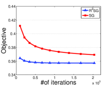
(a) comparison between different algorithms

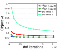
(b) sensitivity to initial solutions

Figure 4: Results for solving SVM classification with GFlassso regularizer. In (b), the objective values of the two initial solutions are $1$ and $70.35$. One iteration means one subgradient update in all algorithms.

8.2 SVM Classification with a graph-guided fused lasso

The classification problem is to predict a binary class label $y\in\{1,-1\}$ based on a feature vector $\mathbf{x}\in\mathbb{R}^{d}$. Given a set of training examples $(\mathbf{x}_{i},y_{i}),i=1,\ldots,n$, the problem of training a linear classification model can be cast into

$$\min_{\mathbf{w}\in\mathbb{R}^{d}}F(\mathbf{w}):=\frac{1}{n}\sum_{i=1}^{n}\ell(\mathbf{w}^{\top}\mathbf{x}_{i},y_{i})+R(\mathbf{w}).$$

Here we consider the hinge loss $\ell(z,y)=\max(0,1-yz)$ as in support vector machine (SVM) and a graph-guided fused lasso (GFlasso) regularizer $R(\mathbf{w})=\lambda\|F\mathbf{w}\|_{1}$ (Kim et al., 2009), where $F=[F_{ij}]_{m\times d}\in\mathbb{R}^{m\times d}$ encodes the edge information between variables. Suppose there is a graph $\mathcal{G}=\{\mathcal{V},\mathcal{E}\}$ where nodes $\mathcal{V}$ are the attributes and each edge is assigned a weight $s_{ij}$ that represents some kind of similarity between attribute $i$ and attribute $j$. Let $\mathcal{E}=\{e_{1},\ldots,e_{m}\}$ denote a set of $m$ edges, where an edge $e_{\tau}=(i_{\tau},j_{\tau})$ consists of a tuple of two attributes. Then the $\tau$-th row of $F$ matrix can be formed by setting $F_{\tau,i_{\tau}}=s_{i_{\tau},j_{\tau}}$ and $F_{\tau,j_{\tau}}=-s_{i_{\tau},j_{\tau}}$ for $(i_{\tau},j_{\tau})\in\mathcal{E}$, and zeros for other entries. Then the GFlasso becomes $R(\mathbf{w})=\lambda\sum_{(i,j)\in\mathcal{E}}s_{ij}|w_{i}-w_{j}|$. Previous studies have found that a carefully designed GFlasso regularization helps in reducing the risk of over-fitting. In this experiment, we follow (Ouyang et al., 2013) to generate a dependency graph by sparse inverse covariance selection (Friedman et al., 2008). To this end, we first generate a sparse inverse covariance matrix using the method in (Friedman et al., 2008) and then assign an equal weight $s_{ij}=1$ to all edges that have non-zero entries in the resulting inverse covariance matrix. We conduct the experiment on the dna data ($n=2000$ and $d=180$) from the libsvm website, which has three class labels. We solve the above problem to classify class 3 versus the rest. The comparison between different algorithms starting from an initial solution with all zero entries for solving the above problem with $\lambda=0.1$ is presented in Figure 4(a). For R²SG, we start from $t_{1}=10^{3}$ and restart it every $10$ stages with $t$ increased by a factor of $1.15$. The initial step sizes for all algorithms are tuned.

We also compare the dependence of R²SG’s convergence on the initial solution with that of SG. We use two different initial solutions (the first initial solution $\mathbf{w}_{0}=0$ and the second initial solution $\mathbf{w}_{0}$ is generated once from a normal Gaussian distribution). The convergence curves of the two algorithms from the two different initial solutions are plotted in Figure 4(b). Note that the initial step sizes of SG and R²SG are separately tuned for each initial solution. We can see that R²SG is much less sensitive to a bad initial solution than SG consistent with our theory.

8.3 Matrix Completion for Collaborative Filtering

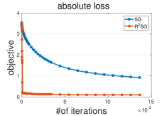
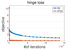
Figure 5: Results for solving low rank matrix completion with different loss functions.

In this subsection, we consider low rank matrix completion problems to demonstrate the effectiveness of R²SG without having the knowledge of $c$ and $\theta$ in the local error bound condition. We consider a movie recommendation data set, namely MovieLens 100k data , which contains $100,000$ ratings from $m=943$ users on $n=1682$ movies. We formulate the problem as a task of recovering a full user-movie rating matrix $X$ from the partially observed matrix $Y$. The objective is composed of a loss function measuring the difference between $X$ and $Y$ on the observed entries and a nuclear norm regularizer on $X$ for enforcing a low rank, i.e.,

$$\min_{X\in\mathbb{R}^{m\times n}}\frac{1}{N}\sum_{(i,j)\in\Sigma}\ell(X_{ij},Y_{ij})+\lambda\|X\|_{*}$$ (25)

where $\Sigma$ is a set of user-movie pairs that denote the observed entries, $\ell(\cdot,\cdot)$ denote a loss function, $\|X\|_{*}$ denotes the nuclear norm, $N=|\Sigma|$ and $\lambda>0$ is a regularization parameter. We consider two loss functions, i.e, the hinge loss and the absolute loss. For absolute loss, we set $\ell(a,b)=|a-b|$. For hinge loss, we follow that in (Rennie and Srebro, 2005) by introducing four thresholds $\theta_{1,2,3,4}$ due to there are five distinct ratings in $\{1,2,3,4,5\}$ that can be assigned to each movie, and defining $\ell(a,b)=\sum_{r=1}^{4}\max(0,1-T^{r}_{i,j}(\theta_{r}-X_{ij}))$, where $T^{r}_{ij}=\left\{\begin{array}[]{cc}1&\text{ if }r\geq Y_{ij}\\ 0&\text{ otherwise}\end{array}\right.$. In our experiment, we set $\theta_{1,2,3,4}=(0,3,6,9)$ and $\lambda=10^{-5}$ following (Yang et al., 2014). Since the loss function and the nuclear norm are both semi-algebraic functions (Yang et al., 2016; Bolte et al., 2014), then the problem (25) satisfies an error bound condition on any compact set (Bolte et al., 2017). However, it remains an open problem what are the proper values of $c$ and $\theta$ to make local error bound condition hold. Hence, we run R²SG by setting $\theta=0$. To compare with SG, we simply set $t_{1}=10$ - the number of iterations of each stage of the first call of RSG. The baseline SG is implemented in the same way as before. The results of the objective values vs the number of iterations are plotted in Figure 5. We can see that R²SG converges much faster than SG, verifying the effectiveness of R²SG predicted by Theorem 16.

8.4 Comparison with Freund & Lu’s SG

In this subsection, we compare the proposed RSG with Freund & Lu’ SG algorithm empirically. The later algorithm is designed with a fixed relative accuracy $\epsilon^{\prime}$ such that $\frac{f(\mathbf{x}_{t})-f_{*}}{f_{*}-f_{slb}}\leq\epsilon^{\prime}$, where $f_{slb}$ is a strict lower bound of $f_{*}$, and requires to maintain the best solution in terms of the objective value during the optimization. For fair comparison, we run RSG with a fixed $t$ and then vary $\epsilon^{\prime}$ for Freund & Lu’s SG algorithm that is an input parameter, and then plot the objective values versus the running time and the number of iterations for both algorithms. The experiments are conducted on the two classification data sets as used in subsection 8.1, namely the housing data and the space-ga data, for solving robust regression problems (19) with $p=1$ and $p=1.5$. The strict lower bound $f_{slb}$ in Freund & Lu’s algorithm is set to $0$. The results are shown in Figure 7 and Figure 7, where SGR refers to Freund & Lu’s SG algorithm with a specified relative accuracy. For each problem instance (a data set and a particular value of $p$), we report two results comparing the objective values vs. running time and the number of iterations. We can see that RSG is very competitive in performance in terms of running time and converge faster than Freund & Lu’s algorithm with a small $\epsilon^{\prime}=10^{-4}$ for achieving the same accurate solution (e.g., with objective gap less than $10^{-10}$).

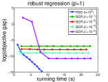
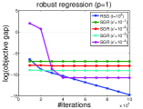
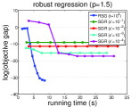
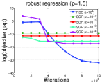
Figure 6: Comparison of RSG with Freund & Lu’s SG algorithm (SGR) on the housing data.

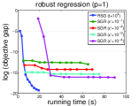
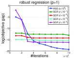
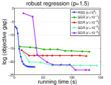
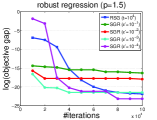
Figure 7: Comparison of RSG with Freund & Lu’s SG algorithm (SGR) on the space-ga data.

9 Conclusion

In this work, we have proposed a novel restarted subgradient method for non-smooth and/or non-strongly convex optimization for obtaining an $\epsilon$-optimal solution. By leveraging the lower bound of the first-order optimality residual, we establish a generic complexity of RSG that improves over standard subgradient method. We have also considered several classes of non-smooth and non-strongly convex problems that admit a local error bound condition and derived the improved order of iteration complexities for RSG. Several extensions have been made to design a parameter-free variant of RSG without requiring the knowledge of the constants in the local error bound condition. Experimental results on several machine learning tasks have demonstrated the effectiveness of the proposed algorithms in comparison to the subgradient method.

Acknolwedgements

We would like to sincerely thank anonymous reviewers for their very helpful comments. We thank James Renegar for pointing out the connection to his work and for his valuable comments on the difference between the two work. We also thank to Nghia T.A. Tran for pointing out the connection between the local error bound and metric subregularity of subdifferentials. Thanks to Mingrui Liu for spotting an error in the formulation of the $F$ matrix for GFlasso in earlier versions. T. Yang is supported by NSF (1463988, 1545995).

A A proposition needed to prove Corollary 14

The proof of Corollary 14 leverages the following result from (Bolte et al., 2017).

Proposition 1

(Bolte et al., 2017, Theorem 5) Let $f(x)$ be an extended-valued, proper, convex and lower semicontinuous function that satisfies the KL inequality (20) at $x_{*}\in\arg\min f(\cdot)$ for all $x\in U\cap\{x:f(x_{*})<f(x)<f(x_{*})+\eta\}$, where $U$ is a neighborhood of $x_{*}$, then $dist(x,\arg\min f(\cdot))\leq\varphi(f(x)-f(x_{*}))$ for all $x\in U\cap\{x:f(x_{*})<f(x)<f(x_{*})+\eta\}$.

References

- Artacho and Geoffroy [2008] Francisco J Arag n Artacho and Michel H Geoffroy. Characterization of metric regularity of subdifferentials. Journal of Convex Analysis, 15:365–380, 2008.
- Attouch et al. [2010] Hédy Attouch, Jérôme Bolte, Patrick Redont, and Antoine Soubeyran. Proximal alternating minimization and projection methods for nonconvex problems: An approach based on the kurdyka-lojasiewicz inequality. Math. Oper. Res., 35:438–457, 2010.
- Attouch et al. [2013] Hedy Attouch, J r me Bolte, and Benar Fux Svaiter. Convergence of descent methods for semi-algebraic and tame problems: proximal algorithms, forward-backward splitting, and regularized gauss-seidel methods. Math. Program., 137(1-2):91–129, 2013.
- Bach [2013] Francis R. Bach. Learning with submodular functions: A convex optimization perspective. Foundations and Trends in Machine Learning, 6(2-3):145–373, 2013.
- Bach and Moulines [2013] Francis R. Bach and Eric Moulines. Non-strongly-convex smooth stochastic approximation with convergence rate o(1/n). In Advances in Neural Information Processing Systems (NIPS), pages 773–781, 2013.
- Bertsimas and Copenhaver [2014] Dimitris Bertsimas and Martin S. Copenhaver. Characterization of the equivalence of robustification and regularization in linear, median, and matrix regression. arXiv, 2014.
- Bolte et al. [2006] Jérôme Bolte, Aris Daniilidis, and Adrian Lewis. The łojasiewicz inequality for nonsmooth subanalytic functions with applications to subgradient dynamical systems. SIAM J. on Optimization, 17:1205–1223, 2006.
- Bolte et al. [2007] Jérôme Bolte, Aris Daniilidis, Adrian S. Lewis, and Masahiro Shiota. Clarke subgradients of stratifiable functions. SIAM Journal on Optimization, 18:556–572, 2007.
- Bolte et al. [2014] Jérôme Bolte, Shoham Sabach, and Marc Teboulle. Proximal alternating linearized minimization for nonconvex and nonsmooth problems. Mathematical Programming, 146:459–494, 2014.
- Bolte et al. [2017] Jérôme Bolte, Trong Phong Nguyen, Juan Peypouquet, and Bruce W. Suter. From error bounds to the complexity of first-order descent methods for convex functions. Mathematical Programming, 165(2):471–507, Oct 2017. doi: 10.1007/s10107-016-1091-6.
- Burke and Deng [2002] James V. Burke and Sien Deng. Weak sharp minima revisited part i: Basic theory. Control and Cybernetics, 31:439?469, 2002.
- Burke and Deng [2005] James V. Burke and Sien Deng. Weak sharp minima revisited, part II: application to linear regularity and error bounds. Math. Program., 104(2-3):235–261, 2005.
- Burke and Deng [2009] James V. Burke and Sien Deng. Weak sharp minima revisited, part III: error bounds for differentiable convex inclusions. Math. Program., 116(1-2):37–56, 2009.
- Burke and Ferris. [1993] James V. Burke and Michael C. Ferris. Weak sharp minima in mathematical programming. SIAM Journal on Control and Optimization, 31(5):1340–1359, 1993. doi: 10.1137/0331063.
- Chen et al. [2012] Xi Chen, Qihang Lin, and Javier Pena. Optimal regularized dual averaging methods for stochastic optimization. In Advances in Neural Information Processing Systems (NIPS), pages 395–403. 2012.
- Drusvyatskiy and Kempton [2016] Dmitriy Drusvyatskiy and Courtney Kempton. An accelerated algorithm for minimizing convex compositions. arXiv:1605.00125, 2016.
- Drusvyatskiy and Lewis [2018] Dmitriy Drusvyatskiy and Adrian S. Lewis. Error bounds, quadratic growth, and linear convergence of proximal methods. Mathematics of Operations Research, 2018.
- Drusvyatskiy et al. [2014] Dmitriy Drusvyatskiy, Boris Mordukhovich, and Nghia T.A. Tran. Second-order growth, tilt stability, and metric regularity of the subdifferential. Journal of Convex Analysis, 21:1165–1192, 2014.
- Eremin [1965] I. I. Eremin. The relaxation method of solving systems of inequalities with convex functions on the left-hand side. Dokl. Akad. Nauk SSSR, 160:994 – 996, 1965.
- Ferris [1991] Michael C. Ferris. Finite termination of the proximal point algorithm. Mathematical Programming, 50(1):359–366, Mar 1991.
- Freund and Lu [2017] Robert M. Freund and Haihao Lu. New computational guarantees for solving convex optimization problems with first order methods, via a function growth condition measure. Mathematical Programming, 2017.
- Friedman et al. [2008] Jerome Friedman, Trevor Hastie, and Robert Tibshirani. Sparse inverse covariance estimation with the graphical lasso. Biostatistics, 9, 2008.
- Ghadimi and Lan [2013] Saeed Ghadimi and Guanghui Lan. Optimal stochastic approximation algorithms for strongly convex stochastic composite optimization, II: shrinking procedures and optimal algorithms. SIAM Journal on Optimization, 23(4):2061–2089, 2013.
- Gilpin et al. [2012] Andrew Gilpin, Javier Peña, and Tuomas Sandholm. First-order algorithm with log(1/epsilon) convergence for epsilon-equilibrium in two-person zero-sum games. Math. Program., 133(1-2):279–298, 2012.
- Goebel and Rockafellar [2007] R. Goebel and R. T. Rockafellar. Local strong convexity and local lipschitz continuity of the gradient of convex functions. Journal of Convex Analysis, 2007.
- Gong and Ye [2014] Pinghua Gong and Jieping Ye. Linear convergence of variance-reduced projected stochastic gradient without strong convexity. CoRR, abs/1406.1102, 2014.
- Hazan and Kale [2011] Elad Hazan and Satyen Kale. Beyond the regret minimization barrier: an optimal algorithm for stochastic strongly-convex optimization. In Proceedings of the 24th Annual Conference on Learning Theory (COLT), pages 421–436, 2011.
- Hou et al. [2013] Ke Hou, Zirui Zhou, Anthony Man-Cho So, and Zhi-Quan Luo. On the linear convergence of the proximal gradient method for trace norm regularization. In Advances in Neural Information Processing Systems (NIPS), pages 710–718, 2013.