Nonlinear Bound States in a Schödinger-Poisson System with External Potential

Abstract.

We consider radial solutions to the Schrödinger-Poisson system in three dimensions with an external smooth potential with Coulomb-like decay. Such a system can be viewed as a model for the interaction of dark matter with a bright matter background in the non-relativistic limit. We find that there are infinitely many critical points of the Hamiltonian, subject to fixed mass, and that these bifurcate from solutions to the associated linear problem at zero mass. As a result, each branch has a different topological character defined by the number of zeros of the radial states. We construct numerical approximations to these nonlinear states along the first several branches. The solution branches can be continued, numerically, to large mass values, where they become asymptotic, under a rescaling, to those of the Schrödinger-Poisson problem with no external potential. Our numerical computations indicate that the ground state is orbitally stable, while the excited states are linearly unstable for sufficiently large mass.

1. Introduction

We consider the existence and stability of stationary solutions to the radial, focusing nonlinear Schrödinger-Poisson equation in $\mathbf{R}^{3}$ with focusing, Coulomb-like potential,

(1.1) $$i\partial_{t}\phi-\Delta\phi+V(|x|)\phi-{\mathcal{N}}(\phi)=0.$$

Under the ansatz $\phi(x,t)=e^{-iEt}u(x)$, the stationary solution, $u$, satisfies a nonlinear elliptic equation with nonlocal nonlinearity and long range potential function. The time independent problem takes the form:

(1.2) $$-\Delta u+V(|x|)u-{\mathcal{N}}(u)=-Eu.$$

Throughout, the external potential $V$ will be the solution of

(1.3) $$\Delta V=\rho(|x|)$$

for $\rho>0$, $\|\rho\|_{L^{1}}=Z$. The techniques developed here, analytically and numerically, can be modified to include the case $\rho=Z\delta(x)$, corresponding to the classic Coulomb potential, $-Z/|x|$. Nonlinear Schrödinger equations, like (1.1), with other external attractive, singular, potentials have also been considered in quantum mechanical applications. For instance, a $-r^{-2}$ potential, together with a harmonic trapping potential and a repulsive nonlinearity, was examined under spherical and cylindrical symmetry in [25, 24]. While similar methods to those applied here could be implemented in such cases, due to our interest in the application to general relativity we have focused on $r^{-1}$-type potentials. We will take an attractive nonlinearity ${\mathcal{N}}(u)$ to be of Schrödinger-Poisson type, given by

(1.4) $$\mathcal{N}(u)=(|x|^{-1}*|u|^{2})u=[(-\Delta)^{-1}|u|^{2}]u,$$

where $(|x|^{-1}*|u|^{2})$ corresponds to the convolution of $|u|^{2}$ with the standard Green’s function in $\mathbf{R}^{3}$. This nonlinearity is sub-critical with respect to the $L^{2}$ scaling and nonlocal. In this case, (1.2) is the Euler-Lagrange equation for the energy functional

(1.5) $$\mathcal{H}(u)=\int|\nabla u|^{2}dx+\int V|u|^{2}dx-\frac{1}{2}\int\frac{|u|^{2}(x)|u|^{2}(y)}{|x-y|}dxdy,$$

subject to fixed mass

(1.6) $$\mathcal{M}(u)=\int|u|^{2}dx,$$

and $E$ plays the role of the Lagrange multiplier.

The nonlocal nonlinearity, (1.4), arises in the non-relativistic limit of an Einstein-Klein-Gordon system, which can serve as a model for Dark Matter, [3]. Following an idea of Bray, this potential allows us to model the trapping of Dark Matter by “bright matter.” The potential is itself a solution to $\Delta V=\rho$ for mass density $\rho$. In a general relativistic model proposed by Bray and others, stable excited states of the Einstein-Klein-Gordon system including a background matter potential representing the “bright matter” have been sought, [4, 5]. This is modeled by adding a mass density to the Einstein-Klein-Gordon equations, which plays the role of the potential, $V$, in the Schrödinger-Poisson model studied here.

Many of our results are applicable to other potentials and nonlinearities, but we focus on Coulomb and Schrödinger-Poisson. For instance, we might also study both super-critical and sub-critical local nonlinearities, including the classical cubic nonlinearity,

(1.7) $$\mathcal{N}(u)=|u|^{2}u,$$

and a nonlinearity popular in density functional theory, representing a Dirac exchange term,

(1.8) $$\mathcal{N}(u)=|u|^{\frac{2}{3}}u.$$

See [1] for how such an attractive nonlinearity arises in the LDA functional in density functional theory. In all cases we consider, the nonlinearities are assumed to be focusing and the external potentials are assumed to be attractive. The most significant differences amongst the cases will appear in the large $E$ asymptotics. Additional care in the analysis will also be required for potentials which are not smooth, as in the pure Coulomb potential for instance, along with non-smooth nonlinearities, such as (1.8).

Here, we prove the existence of branches of radially symmetric solutions to our system. Each branch, as a function of the mass, corresponds to solutions with a particular number of zero crossings in the radial coordinate, and this number is invariant along the branch. At mass zero, the branches terminate in the eigenstates associated with the linear operator $-\Delta+V$. Continuing the branches requires a spectral assumption. Specifically, we assume that

Assumption 1.

The kernel of the linearization of (1.2), about a given solution, restricted to radial functions, is trivial.

In our numerical computations, we found that the discretized operator did not have a kernel.

We are able to show that, at the very least, none of the branches intersect. In addition, we explore the high energy limit ($E\to\infty$), showing that these branches, should they continue all the way to $E\to\infty$, connect to solutions of (1.2) with $V=0$. We also examine the stability of the bound states, both through a numerical examination of the spectrum, and through time dependent simulations. We find the ground state to be orbitally stable, while the excited states, of sufficiently large $E$, are linearly unstable.

Our work is organized as follows. In Section 2, we review properties of the spectrum with Coulomb potentials and establish the properties needed for a bifurcation analysis. Next, in Section 3, we use a Lyapunov-Schmidt reduction to construct a branch of bound states emanating from each linear eigenvalue involving projection onto all the other discrete spectral modes. We then discuss how such branches behave as the nonlinear eigenvalue $E\to\infty$, in Section 4. In Section 5, we review orbital stability and relate it to our problem. Then, in Section 6, we describe the numerical methods we have used and present the results from various time-dependent simulations and spectral stability calculations. In Section 7, we discuss our calculations and simulations, along with open problems. Some additional bounds on unstable eigenvalues are given in Appendix A

2. Review of Linear Spectral Theory

In this section, we review some key results from linear spectral theory for operators of the form of $H=-\Delta+V$.

2.1. The Hydrogen Atom

Recall that $V=-Z/|x|$ corresponds to the well known model of the hydrogen atom, for which the eigenvalues and eigenfunctions are entirely explicit; see [11]. The solutions to

(2.1) $$-\Delta\psi_{E}-\frac{Z}{|x|}\psi_{E}=-E\psi_{E}$$

can be obtained by power series methods, with eigenvalues

(2.2) $$E=E_{n}\equiv\frac{Z^{2}}{2n^{2}},\ \ n\in\mathbf{N},$$

and corresponding radial eigenfunctions

(2.3) $$\psi_{n}(x)=e^{-\frac{Z|x|}{n}}P_{n-1}(\tfrac{Z|x|}{n}).$$

Here, the $P_{n}(s)$ are the Laguerre polynomials $L_{n}^{1}(s)$. Each $P_{n}$ has precisely $n$ positive zeros, hence $\psi_{n}$ has the corresponding number of roots.

2.2. Potentials with Coulomb like Decay at Infinity

We will use variational methods to obtain the existence of infinitely many radial excited states, with a sequence of eigenvalues approaching zero from below. For more on this type of analysis, see [23, 17].

Proposition 2.1.

Assume that $V(x)$ is spherically symmetric and in $C^{\infty}$, and assume that $\exists Z\in\mathbf{R}^{+}$ such that

(2.4) $$\lim_{|x|\to\infty}|x|V(x)=-Z.$$

Then $L=-\Delta+V(x)$, interpreted as a linear operator with form domain $H^{1}_{\operatorname{rad}}(\mathbf{R}^{3})$, has an increasing infinite sequence of negative eigenvalues that approaches zero from below.

Proof.

Let $L_{0}=-\Delta$. We apply the Rayleigh-Ritz technique, as in Section XIII.2 of Reed-Simon, to find the claimed infinite set of eigenvalues.

Define

(2.5) $$\mu_{n}(L):=\sup_{\begin{subarray}{c}S\subset H,\\ \mathrm{dim}(S)=n-1\end{subarray}}\inf_{\begin{subarray}{c}\psi\in S^{\perp},\\ \|\psi\|=1\end{subarray}}\langle\psi,L\psi\rangle.$$

Note that $L$ is bounded from below because $V$ is bounded and $L_{0}$ is a nonnegative operator. Therefore, it follows that if $P$ is a projection onto any $n$-dimensional subspace of $H$, then $\mu_{n}$ is bounded from above by the $n$-th eigenvalue of $PLP$ on $S$. (Theorem XIII.3 of [23]). Define the Rollnik class of potentials, $\mathcal{R}$, by

(2.6) $$\mathcal{R}\equiv\left\{V:\mathbf{R}^{3}\to\mathbf{R}\mid\displaystyle\int\frac{|V(x)||V(y)|}{|x-y|^{2}}dxdy<\infty\right\}.$$

Also, define $(L^{\infty})_{\epsilon}$ to be the set of functions with $L^{\infty}$ norm bounded by $\epsilon$. As in Example $7$ on page $118$ of [23], if $V\in\mathcal{R}+(L^{\infty})_{\epsilon}$, $\forall\epsilon>0$, then $-\Delta+V$ is a form-compact perturbation of $L_{0}$ and therefore shares the same essential spectrum. Coulomb potentials belong to the Rollnik class when cut off on any compact set. Therefore, since the remainder is an arbitrarily small bounded perturbation, the Coulomb potential is in the class $\mathcal{R}+(L^{\infty})_{\epsilon}$. By standard Fourier analysis and a spectral perturbation argument, the essential spectrum of $L_{0}$ can be shown to be $[0,\infty)$. In particular, zero is the bottom of the essential spectrum.

By Theorem XIII.1 of [23], $\forall n\in\mathbf{N}$, $\mu_{n}$ is either the $n$-th eigenvalue of $L$ or $\mu_{n}=0$, the base of the essential spectrum. Provided we can show that $\mu_{n}<0\ \forall n\in\mathbf{N}$, we can conclude that $L$ has infinitely many eigenvalues. To do this, for each $n$ we will find appropriate $n$-dimensional spaces $H_{n}$ on which all eigenvalues are negative, and then apply the above described upper bound.

This argument appears in the proof of Theorem XIII.6 of [23]. Choose $\psi\in C_{0}^{\infty}(\mathbf{R}^{3})$ satisfying $\psi\geq 0$ and supp$(\psi)\subset\{x:1<|x|<2\}$, $\psi$ is radially symmetric and $\|\psi\|_{L^{2}}=1$. Define $\psi_{R}(x)=R^{-\frac{3}{2}}\psi(\frac{x}{R}).$ Then supp$(\psi_{R})\subset\{x:R<|x|<2R\}$ and $\psi_{R}$ satisfies the other conditions above. For $R$ sufficiently large,

$$\langle\psi_{R},L\psi_{R}\rangle =\langle\psi_{R},-\Delta\psi_{R}\rangle-\langle\psi_{R},V(x)\psi_{R}\rangle\leq\langle\psi_{R},-\Delta\psi_{R}\rangle-\langle k\psi_{R},{|x|^{-1}}\psi_{R}\rangle$$

$$\quad\leq R^{-2}\langle\psi,-\Delta\psi\rangle-kR^{-1}\langle\psi,\psi\rangle<0.$$

Fix $R_{0}$ sufficiently large so that this is true whenever $R>R_{0}$ Now let $\phi_{m}=\psi_{2^{m}R_{0}}$ for $m=1\ldots n$. It follows that, on $H_{n}=\mathrm{span}\{\phi_{1},\ldots,\phi_{n}\}$, all eigenvalues of $PLP$ are negative, because these functions have disjoint support. Hence $L$ has an infinite sequence of negative eigenvalues approaching zero from below. ∎

2.2.1. Sturm-Liouville Theory

Let $(-E_{n},\psi_{n})$ be the eigenpairs for $L$ on $H$, ordered so that $-E_{n}$ increases as $n$ increases. We would like to know that, if $-E_{m}>-E_{n}$, then $\psi_{m}$ has more zero crossings than $\psi_{n}$. This requires a Sturm-Liouville-type argument on the radial equation satisfied by the eigenfunctions. We first need a preliminary lemma about the decay rate of our eigenfunctions:

Lemma 2.1.

For each $n$, $\psi_{n}$ has exponential decay as $r$ tends to infinity.

Proof.

To see this, first let $\phi=r\psi_{n}$. Then $\phi$ satisfies

$$-\phi^{\prime\prime}+V\phi=-E_{n}\phi.$$

The proof follows directly from the asymptotic analysis of second order linear systems in [6], Chapter $3$, Theorem $8.6$. In particular, this linear system can be seen to have two solutions as $r\to\infty$, one of which is exponentially decaying and one of which is exponentially growing and converging to the rate of decay . As a result, since an eigenfunction has decay, we observe that for a sufficiently large $R>0$ that

$$\lim_{r\to\infty}\phi(r)e^{\int_{R}^{r}\sqrt{E_{n}+V(s)}}ds=c$$

for some constant $c$. ∎

Now, define $N_{n}$ to be the number of zeroes of $\psi_{n}$. We will now prove the following:

Proposition 2.2.

Under the same assumptions as above, whenever $-E_{m}>-E_{n}$, $N_{m}\geq N_{n}+1$.

Proof.

After the transformation in the proof of Lemma 2.1 this is a consequence of standard Sturm-Liouville theory in dimension one, see for instance the treatment in [6]. ∎

Finally, we would like to confirm that each of these eigenvalues is simple within $H^{1}_{\operatorname{rad}}$.

Proposition 2.3.

Each eigenvalue $E_{n}$ of the operator $H=-\Delta+V$, $\Delta V=\rho(|x|)$ with $\|\rho\|_{L^{1}}=Z$ in the class of radial functions, $H^{1}_{\operatorname{rad}}$, is simple.

Proof.

Again, this follows from Sturm-Liouville Theory once the transformation in the proof of Lemma 2.1 is used. ∎

3. Existence of Nonlinear Bound States

We now prove the existence of nonlinear solutions bifurcating from zero mass off of each discrete linear eigenvalue. We will follow the argument in Kirr-Kevrekidis-Schlizerman-Weinstein [15] to obtain such bifurcation curves. First let us construct the individual bifurcation branches.

Theorem 1.

For a given $n\in\mathbf{N}$, let $(-E_{n},\psi_{n})$ be a simple eigenpair of $L:=-\Delta+V(x)$ in $H^{1}_{\operatorname{rad}}$, let $P$ be the projection onto the eigenspace, i.e. $Pu=\langle u,\psi\rangle\psi$, and let $Q=I-P$ be the spectral projection onto the rest of the spectrum of $L$. Define $\delta=\frac{1}{2}\min\{|\mu-E_{n}|:\mu\in\sigma(L)\},$ and let $E$ be such that $0<E-E_{n}<\delta$. Then, there exists a solution $u_{E}\in H^{1}_{\operatorname{rad}}$ to (1.2) with the same number of zero crossings as $\psi$.

Proof.

We seek nontrivial radial solutions $u$ to (1.2), where $\|u\|_{L^{2}}$ is small, and therefore we expect that $u\sim c_{0}\psi_{n}$ and $E-E_{n}\sim 0$ for $c_{0}$ also small. For brevity, we write $\psi$ for $\psi_{n}$ in what follows. In order to find $u$, we make the ansatz $u=c_{0}\psi+\eta$ with $Q\eta=\eta$. Substituting into (1.2), we obtain

$$-\Delta(c_{0}\psi+\eta)+V(r)(c_{0}\psi+\eta)-\left(\frac{1}{r}\ast|(c_{0}\psi+\eta)|^{2}\right)(c_{0}\psi+\eta)=E(c_{0}\psi+\eta).$$

Using the fact that $-\Delta\psi+V(r)\psi=-E_{n}\psi$ and that

$$Q(-\Delta+V(x)+E)\psi=Q(E-E_{n})\psi=0,$$

we obtain

$$c_{0}(E-E_{n})\psi-P{\mathcal{N}}(c_{0}\psi+\eta) =0$$

$$(-\Delta+V(x)+E)\eta-Q{\mathcal{N}}(c_{0}\psi+\eta) =0$$

where ${\mathcal{N}}(f)=(\frac{1}{r}*|f|^{2})f$. Note that $\|{\mathcal{N}}(f)\|_{L^{2}}\leq k\|f\|_{H^{2}}^{3}$ for some $k>0$, and that ${\mathcal{N}}$ is a real analytic function in each argument. We will choose parameters $\nu,\rho$ later and we require that $|c_{0}|<\nu$, $\|u\|_{H^{2}}<\rho$, and $|E-E_{n}|<\delta$. Within this open set, $(L-E_{n})^{-1}Q$ is an analytic map from $L^{2}$ to $H^{2}$ with norm controlled by $\delta$, and hence it follows that

$$\|(L-E_{n})^{-1}Q{\mathcal{N}}(c_{0}\psi+\eta)\|_{H}^{2}\leq C(\delta)\|c_{0}\psi+\eta\|_{H^{2}}^{3},$$

and the map

$$F:=(c_{0},E_{n},\eta)\mapsto(L-E_{n})^{-1}Q{\mathcal{N}}(c_{0}\psi+\eta)$$

is real analytic. Note that $F(0,E_{n},0)=0$ and $DF(0,E_{n},0)=I$. Hence, by the implicit function theorem there exist $\nu$ and $\rho$ so that on the open set described above, there is an analytic solution $\eta(c_{0},E_{n})$ to $\eta-(L-E_{n})^{-1}Q{\mathcal{N}}(c_{0}\psi+\eta)=0$. Note that

$$Q(L-E_{n})^{-1}Q{\mathcal{N}}(c_{0}\psi+\eta)=Q(0)=0,$$

so

$$Q\eta=(H-E_{n})^{-1}Q{\mathcal{N}}=\eta.$$

So $\eta$ lies in the orthogonal projection away from $\psi$ as desired.

Finally, by substituting back into the first equation, we obtain

$$c_{0}(E-E_{n})\psi-P{\mathcal{N}}(c_{0}\psi_{\eta}(c_{0},E_{n}))=0$$

with the condition $|c_{0}|^{2}+\|\eta(c_{0},E_{n})\|_{L^{2}}^{2}=\epsilon$ for small fixed $\epsilon$. Projecting onto $\psi$, we have that

$$E-E_{n}-|c_{0}|^{2}a-\frac{1}{c_{0}}\langle\psi,{\mathcal{N}}(c_{0}\psi+\eta)-{\mathcal{N}}(c_{0}\psi)\rangle=0$$

where $a=\langle\psi,{\mathcal{N}}(\psi)\rangle$. By the implicit function theorem again, we obtain that there is a differentiable function $h$ so that $E=h(c_{0})$ in the allowed open interval. We may conclude that the desired solution $u_{E}$ exists for $E$ on this curve. Note that $h^{\prime}(0)>0$, so that $E>E_{n}$ in this regime. ∎

It follows that there is a bifurcation branch from each eigenvalue of the linear problem. As the spectral gap, measured by the number $\delta$ in the above result, decreases, the range of $E$ for which the theorem holds will be reduced.

We are also interested in the continuation of our branches away from the zero mass limit, where we know they exist. In particular, we would like to know that they continue as $E\to+\infty$, and that the branches do not intersect.

First, consider the matter of large values of $E$. Define $(\psi_{j},E_{j})$ to be the radial, normalized Coulomb eigenpairs of the linear operator. From Theorem 1 we have a $j$-th branch for $E>E_{j}$, branching from $\psi_{j}$ at the zero mass limit. For each branch, we follow [14], where smooth potentials are treated in dimension one, and use the regularity of bound states with Coulomb potentials from [18]. Then, the Euler-Lagrange equations can be seen as a map on $H^{2}$ functions given by

(3.1) $$F(Z,E;u)=-\Delta u+Eu+V(|x|)u-(|x|^{-1}*|u|^{2})u=0.$$

Consequently, away from mass zero (or for values of $E>E_{j}$), we can apply the implicit function theorem directly to $F$ at $(E,u_{E})$ to construct a $C^{1}$ family of solutions $u_{E}\in H^{2}$ space under the assumption that the linearization of the equation about solution $u_{E}$,

$$L_{+}=-\Delta+V(|x|)+E-(|x|^{-1}*|u_{E}|^{2})-2(|x|^{-1}*(u_{E}\bullet))u_{E},$$

has no kernel. This is Assumption 1 from the introduction. See the work [17] for a general treatment of this problem with $V=0$, where it is proven in their Proposition $2$ that for the ground state Hartree soliton, the kernel of $L_{+}$ is trivial in the space of radial functions. We observe numerically below (see Figure 6) that each of our branches can be continued. Using the same techniques as in Section 6, we found, numerically, that the discretized $L_{+}$ operator lacks a kernel.

Moreover, the branches cannot cross. Indeed, if two branches crossed, then there would be a transition from a family of solutions with more zeroes to one of fewer zeroes. As a result, if this were to occur at some point $r\geq 0$ along the curve, there would be a nonlinear bound state with both value and derivative being $0$. By ODE uniqueness theory, this would be a trivial solution. Thus, we conclude that if we were unable to continue a given branch in $E$, it would not be due to branches crossing.

We note that, by the arguments for the proof of Theorem $1$ of [19], for each $E>E_{0}$, there are an infinite number of radial solutions with increasing energy. As a result, we in the next Section analytically and numerically consider the behavior of solutions as $E\to\infty$, so long as our spectral assumption is met and such branches can be continued.

4. Limiting Behavior as $E\to\infty$

Following in the spirit of Section $4$ of [14], in this section we consider the case $E\to\infty$ provided the lowest energy solution branch can be uniquely continued. The analytic results here will apply to large $E$ behavior of the ground state branch, for the generalized Coulomb-like equation

(4.1) $$-\Delta u+Eu+V(|x|)u-(|x|^{-1}*|u|^{2})u=0,\ \ \Delta V=\rho,\ \ \int\rho dx=Z,$$

but with appropriate modifications a similar approach will apply to

(4.2) $$-\Delta u+Eu-\frac{Z}{|x|}u-(|x|^{-1}*|u|^{2})u=0.$$

For the excited states, we lack a rigorous result on the kernel of the linearized operator in the large $E$ limit. Conditional on this having trivial kernel, we can apply the same argument as in the case of the ground state.

Without the external potential, the problem

(4.3) $$-\Delta\phi+E\phi-(|x|^{-1}*|\phi|^{2})\phi=0$$

is solved by the $\phi_{E}=E\phi_{1}(\sqrt{E}x)$ where

(4.4) $$-\Delta\phi_{1}+\phi_{1}-(|x|^{-1}*|\phi_{1}|^{2})\phi_{1}=0.$$

Substituting the scaling $u=E\tilde{u}(\sqrt{E}x)$ into our problem, we obtain

(4.5) $$-\Delta\tilde{u}+\tilde{u}+\frac{1}{E}V\left(\frac{x}{\sqrt{E}}\right)\tilde{u}-(|x|^{-1}*|\tilde{u}|^{2})\tilde{u}=0.$$

Note that in the pure Coulomb case we have $V\left(x/{\sqrt{E}}\right)/E=-Z/(\sqrt{E}|x|)$, meaning that away from zero, the potential is tending to zero, pointwise. We wish to show that $\tilde{u}$ is close to $\phi_{1}$ as $E\to\infty$ by using the fact that the rescaled, smoothed Coulomb potential vanishes pointwise.

Making the ansatz $\tilde{u}=\phi_{1}+w$,

(4.6) $$\begin{split}\tilde{L}w&=\mathcal{L}_{+}w+\frac{1}{E}V\left(\frac{x}{\sqrt{E}}\right)w\\ &=-\frac{1}{E}V\left(\frac{x}{\sqrt{E}}\right)\phi_{1}+{\mathcal{N}}(\phi_{1},w),\quad{\mathcal{N}}=O(\phi_{1}w^{2})+O(w^{3}),\end{split}$$

where

(4.7) $$\mathcal{L}_{+}w=-\Delta w+w-\left(\int\frac{|\phi_{1}|^{2}(y)}{|x-y|}dy\right)w-2\left(\int\frac{\phi_{1}w}{|x-y|}dy\right)\phi_{1}.$$

By results found in [17, Proposition $2$, Appendix $A$], there is a unique radial ground state $\phi_{1}$, which is positive and exponentially decaying everywhere. Furthermore, $\mathcal{L}_{+}$ is self-adjoint and non-degenerate with trivial kernel in the space of radial functions.

For the class of bounded Coulomb potentials under consideration, since $V\in L^{\infty}$, the multiplication operator $w\mapsto\frac{V(\frac{x}{\sqrt{E}})}{E}w$ is compact on $H^{1}$, with norm at most $\frac{\|V\|_{L^{\infty}}}{E}$. We also have that $V\in L^{2}+(L^{\infty})_{\epsilon}$, therefore, $\tilde{L}$ is a relatively compact perturbation of the operator $\mathcal{L}_{+}$; see Example $6$ on page $117$ of [23].

We have that $\tilde{L}$ is invertible on $H^{1}$ for sufficiently large $E$ with an operator norm that is a perturbation of that of $\mathcal{L}^{+}$. Since $\tilde{L}^{-1}:H^{1}\to H^{1}$ is bounded, we have that $\|\tilde{L}^{-1}\mathcal{N}(\phi_{1},w)\|_{H^{1}}\leq C(\left\|w\right\|_{H^{1}}^{2}+\left\|w\right\|_{H^{1}}^{3})$, while

$$\left\|\tilde{L}^{-1}\left(\tfrac{1}{E}V\left(\tfrac{x}{\sqrt{E}}\right)\phi_{1}\right)\right\|_{H^{1}}\leq\tfrac{C}{E}.$$

We therefore have that

$$\left\|\tilde{L}^{-1}\left(-\tfrac{1}{E}V\left(\tfrac{x}{\sqrt{E}}\right)\phi_{1}+{\mathcal{N}}(\phi_{1},w)\right)\right\|_{H^{1}}\leq C(E^{-1}+\left\|w\right\|_{H^{1}}^{2}+\left\|w\right\|_{H^{1}}^{3}).$$

At the same time,

$$\begin{split}&\left\|\tilde{L}^{-1}\left({\mathcal{N}}(\phi_{1},w_{1})-{\mathcal{N}}(\phi_{1},w_{2})\right)\right\|_{H^{1}}\\ &\leq C(\left\|w_{1}\right\|_{H^{1}}+\left\|w_{1}\right\|_{H^{1}}^{2}+\left\|w_{2}\right\|_{H^{1}}+\left\|w_{2}\right\|_{H^{1}}^{2})\|w_{1}-w_{2}\|_{H^{1}}.\end{split}$$

Now assume that $w$ is small, for instance, $\operatorname{O}(E^{-1/2})$. Then, by a standard iteration argument, a solution $w$ will be found in $B_{R}(0)\subset H^{1}$, with $R\sim E^{-1/2}$ as $E$ becomes large. To conclude, we can construct solutions along our ground state branch such that $w\to 0$ as $E\to\infty$ and the profile of our solutions approaches $\phi_{1}$ for large $E$ as claimed. See Figure 1 for numerical exploration of this scaling limit, which confirm the desired scaling as $E$ becomes large.

As a side note, one could prove that solutions to (4.1) for a given $E$ have an $L^{2}$ norm indicated by the scalings used above, then as in [14] for the $1d$ case with smooth potential, concentration compactness tools could be used to give a simpler proof of the convergence explored for the ground state branch. However, as the nonlinearity has such nice algebraic properties, we have taken the approach of using elliptic estimates directly.

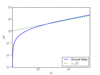
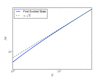
Figure 1. Plots of $E$ vs. mass for large $E$ for the first branch (left) and a zoom in on for large $E$ on the second branch (right). Note, the slope approaches $\tfrac{1}{2}$ on the $\log-\log$ scale.

Remark.

A dividend of this examination of the large $E$ limit is that it provides a strategy for computing excited state solutions for (4.3). While, in practice, one would not solve for $E=\infty$, one could solve Schrödinger-Poisson for large values of $E$, to get, after rescaling, an approximation of the solution to the $V=0$ problem. This preconditioned guess could then be fed to a Newton solver. See [21] for a discussion on computing excited states along with an alternative strategy for obtaining states with a given number of zero crossings.

5. Stability

In the context of the stability works of Grillakis-Shatah-Strauss [10], also known as the Vakhitov-Kolokolov criterion, we consider the problem of orbital stability, restricted to radial functions, of our solution. By orbital stability, we mean that for any $\epsilon>0$, there exists a $\delta$ such that if $\left\|u_{0}-\phi\right\|_{H^{1}}\leq\delta$, then for all $t\geq 0$,

$$\inf_{\theta}\left\|u(t)-e^{i\theta}\phi\right\|\leq\epsilon.$$

Orbital stability makes no claim as to any particular asymptotic behavior.

To proceed, recall that we can write the linearized evolution operator, in terms of real and imaginary parts, as

(5.1) $$H=JL=\begin{pmatrix}0&1\\ -1&0\end{pmatrix}\begin{pmatrix}L_{+}&0\\ 0&L_{-}\end{pmatrix}=\begin{pmatrix}0&L_{-}\\ -L_{+}&0\end{pmatrix},$$

where

(5.2a) $$L_{-} =-\Delta+E+V(x)-(|x|^{-1}|u_{E}|^{2}),{\mbox{ and }}$$

(5.2b) $$L_{+} =-\Delta+E+V(x)-(|x|^{-1}\ast|u_{E}|^{2})-2(|x|^{-1}\ast(u_{E}\bullet))u_{E}.$$

Also, define the scalar function

(5.3) $$d(E)=\mathcal{H}(u_{E})+E\mathcal{M}(u_{E}).$$

Recall then, the results of [10] (see, also, [30, 29, 8, 9, 16]), adapted to this problem. Let $p(d^{\prime\prime}(E))=1$ if $d^{\prime\prime}(E)>0$ and let $p(d^{\prime\prime}(E))=0$ otherwise. Let $n(L)=n(L_{-})+n(L_{+})$ be the number of negative eigenvalues of the operators. Subject to some assumptions on well-posedness of the flow, the existence of the bound states, and the ability to decompose the spectrum of $L$, we have:

Theorem 2 (from [9]).

Assume $d^{\prime\prime}(E)\neq 0$, then

Stability:

If $n(L)=p(d^{\prime\prime})$, the bound state is orbitally stable,

Instability:

If $n(L)-p(d^{\prime\prime})$ is odd, then the soliton is orbitally unstable.

In some important cases, such as NLS with a power nonlinearity, these properties can be deduced analytically; this is the content of some of the formative works on soliton stability. For our problem, however, we must numerically compute the bound state of energy $E$, compute $d^{\prime\prime}(E)$, and then count the number of eigenvalues of the discretized operators $L_{\pm}$.

These computational tasks, detailed below, are readily addressed. Briefly, we find that the ground state soliton is orbitally stable, as is typical for subcritical problems. For the excited states, we find that $n(L)-p(d^{\prime\prime})$ is even in the cases we compute; this case is not addressed by the above theory. We thus perform both direct computation of the spectrum $JL$, as well as time dependent simulations of the excited states with finite perturbations. For sufficienlty large $E$, the excited states appear to be linearly unstable.

To simplify these computations, slightly, we recall from [8, 30] that, for nonlinear bound states in one parameter, an important identity can be obtained for $d^{\prime\prime}(E)$. Observe that, in general,

$$d^{\prime}(E)=\left(\frac{\delta\mathcal{H}}{\delta u},\partial_{E}u_{E}\right)+\mathcal{M}(u_{E})+E\left(\frac{\delta\mathcal{M}}{\delta u},\partial_{E}u_{E}\right).$$

Since the variations are evaluated at $u_{E}$, and $u_{E}$ satisfies the PDE,

(5.4) $$d^{\prime}(E)=\mathcal{M}(\phi_{E}).$$

Thus, $d^{\prime\prime}(E)>0$ if and only if $\mathcal{M}(u_{E})$ is a decreasing function in $E$ corresponding to the Vakhitov-Kolokolov criterion. In our computations, we find that, in all cases examined, $d^{\prime\prime}(E)>0$; $\mathcal{M}(u_{E})$ is an increasing function of $E$.

6. Numerical Computation of Bound States and Stability

Our approach to computing the nonlinear bound states to (1.2) is to start with a bound state with the desired number of zero crossings for the associated linear problem

(6.1) $$-\Delta u+V(|x|)u=-Eu,\quad\left\|u\right\|_{L^{2}}=1.$$

We then perform numerical continuation to obtain the desired nonlinear bound state. During the continuation, the number of zero crossings is invariant.

While it is convenient to think of the linear bound state as the zero mass limit of the nonlinear bound state, this is impractical for numerical continuation. Instead, we augment (1.2) with the artificial continuation parameter, $\gamma\in[0,1]$, to become

(6.2) $$-\Delta u+V(|x|)u-\gamma\mathcal{N}(u)=-Eu,\quad$$

Then, along a sequence of $\gamma$ values,

$$0=\gamma_{0}<\gamma_{1}<\ldots<\gamma_{n_{\gamma}-1}=1,$$

$(u^{(i)},E^{(i)})$ pairs are computed, all with $L^{2}$ norm of unity.

Once the value at $\gamma=1$ is obtained, the mass constraint is relaxed, and $E$ is varied to determine, for instance, $d^{\prime\prime}(E)$. At each value of $E$, the eigenvalues of matrix discretizations of $L_{\pm}$ are computed.

For concreteness, $V$ is the smooth radial function solving

(6.3) $$\Delta V=\frac{1}{2}e^{-r},\quad V(r)=\frac{1}{2}e^{-r}-\frac{1}{r}(1-e^{-r}).$$

6.1. Computation of the Linear States

To begin with, we compute the eigenvalues of (6.1) using its associated weak form and piecewise linear, radial finite elements. A Neumann condition is applied at the origin, and a “big box” homogeneous Dirichlet approximation is made at $r_{\max}$, assumed to be sufficiently large. For $\lambda>0$, the states will be exponentially localized, so this is a reasonable approximation. However, since the point spectra tend to zero, the decay rates at the $n$th eigenvalue of the order, $\propto r^{n}\exp(-\sqrt{\lambda}r)$ will demand ever larger values of $r_{\max}$ in order to be well approximated. For this reason, we will only consider the first few eigenstates.

For a fixed $r_{\max}$, the corresponding linear system is

(6.4) $$\underbrace{{\bf K}_{\rm Dir.}}_{\text{Stiffness Matrix}}+\underbrace{{\bf V}_{\rm Dir.}}_{\text{Potential Matrix}}=-\lambda\underbrace{{\bf M}_{\rm Dir.}}_{\text{Mass Matrix}}.$$

Recall that since our basis is the set of hat functions, $\{\varphi_{i}\}$, on $[0,r_{\max})$,

$$({{\bf K}_{\rm Dir.}})_{ij}=\int_{0}^{r_{\max}}\varphi_{i}^{\prime}(r)\varphi_{j}^{\prime}(r)r^{2}dr,\quad({{\bf V}_{\rm Dir.}})_{ij}=\int_{0}^{r_{\max}}V(r)\varphi_{i}(r)\varphi_{j}(r)r^{2}dr,$$

$$\quad({{\bf M}_{\rm Dir.}})_{ij}=\int_{0}^{r_{\max}}\varphi_{i}(r)\varphi_{j}(r)r^{2}dr.$$

${\bf V}_{\rm Dir.}$ is computed using numerical quadrature. The eigenstates are then computed, as illustrated in Figure 2. Since the states are highly localized, we use a nonuniform mesh, given by

(6.5) $$r_{j}=\sinh(\xi_{j}),\quad\xi_{j}=j\delta\xi,\quad\delta\xi=\frac{\operatorname{arcsinh}{r_{\max}}}{N},\quad j=0,\ldots,n.$$

This spaces the nodes linearly near the origin and exponentially further apart as $j$ increases.

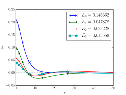
Figure 2. The ground state and the first few excited states of the associated linear problem, (6.1), with $V(r)$ given by (6.3). Computed using (6.4) on the mesh given by (6.5) with $n=4000$ and $r_{\max}=100$.

6.2. Computation of the Nonlinear States

Given the solution to the linear problem at $\gamma=0$, we must now use a nonlinear solver to obtain the desired solution at $\gamma=1$. This is performed using the Python implementation of [26] to solve (6.2). This software is available at https://pythonhosted.org/scikits.bvp_solver/.

6.2.1. First Order System

To use this software package, we must first reformulate our problem as a first order system, with associated boundary conditions. We first remove the nonlocality, by writing our problem as a system of constrained second order equations:

(6.6a) $$Eu-u^{\prime\prime}-\frac{2}{r}u^{\prime}+V(r)u-wu=0,$$

(6.6b) $$-w^{\prime\prime}-\frac{2}{r}w^{\prime}={|u|}^{2},$$

(6.6c) $$\int_{0}^{\infty}|u|^{2}r^{2}dr=1$$

This is then transformed into the aforementioned first order system, with $v=u^{\prime}$, $z=w^{\prime}$, and $m(r)$ being the accumulated mass in $[0,r]$.

(6.7) $$\frac{d}{dr}\begin{pmatrix}u\\ v\\ w\\ z\\ m\end{pmatrix}=\frac{1}{r}\begin{bmatrix}0&0&0&0&0\\ 0&-2&0&0&0\\ 0&0&0&0&0\\ 0&0&0&-2&0\\ 0&0&0&0&0\end{bmatrix}\begin{pmatrix}u\\ v\\ w\\ z\\ m\end{pmatrix}+\begin{pmatrix}v\\ V(r)u-\gamma wu+Eu\\ z\\ -|{u}|^{2}\\ u^{2}r^{2}\end{pmatrix}$$

In the above expressions, we will use $V(r)$ as given by (6.3).

6.2.2. Boundary Conditions

It is now necessary to specify boundary conditions for (6.7). First, we have the natural boundary conditions that $u$ and $w$ be radially symmetric functions. Furthermore, the mass density, $m(r)$, must be zero at the origin. This yields the following three boundary conditions:

(6.8) $$u^{\prime}(0)=v(0)=0,\quad w^{\prime}(0)=z(0)=0,\quad m(0)=0.$$

Next, since the computation is performed on a large, but finite, domain, suitable approximate boundary must be imposed at $r=r_{\max}$. First, we observe that, since $u$ is localized, we can enforce the fixed mass condition by approximating

(6.9) $$m(r_{\max})=\int_{0}^{r_{\max}}|u|^{2}r^{2}dr=1.$$

Next, we first write the equation for $w$ as

$$(w^{\prime}r^{2})^{\prime}=-r^{2}|u|^{2}\Rightarrow w^{\prime}(r)=-\frac{m(r)}{r^{2}}.$$

Since, for large $r$, $m(r)$ is approximately constant, we have

$$w(r)\approx\frac{m(r_{\max})}{r}.$$

This gives rise to our next approximate boundary condition,

(6.10) $$z(r_{\max})+\frac{1}{r_{\max}}w(r_{\max})=0.$$

Finally, at large $r$,

(6.11) $$0\approx Eu-u^{\prime\prime}-\frac{2}{r}u^{\prime}+Vu-wu\approx Eu-u^{\prime\prime}-\frac{2}{r}u^{\prime}-\frac{1}{r}u-\frac{m(r_{\max})}{r}u$$

and we arrive at the approximate Robin condition

(6.12) $$v(r_{\max})+\left(\frac{1}{r_{\max}}+\sqrt{E}-\frac{1+m(r_{\max})}{2r_{\max}\sqrt{E}}\right)u(r_{\max})=0$$

The reader may ask, why, in (6.10) and (6.12), we have not replaced $m(r_{\max})$ by one, as in (6.9). The reason is that, in the first stage of our computation, we will solve for $E$, as an unknown, at fixed $L^{2}$-mass. Subsequently, we will allow $E$ to be a specified parameter, and $L^{2}$ will be an unknown. When $E$ is specified, we discard (6.9), but continue to use (6.10) and (6.12), with $m(r_{\max})$ an unknown that is solved for.

6.2.3. Fixed Mass Profiles

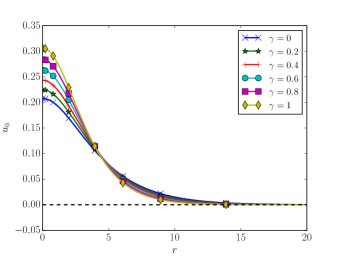
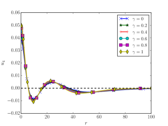
Figure 3. Some of the solutions computed during continuation of $\gamma$ from zero to one in (6.2). In all computed cases, the number of zero crossings was invariant during the continuation.

For mass fixed at one, our continuation strategy produces the sequence of solutions indicated in Figure 3 for the ground state and an excited state with four zero crossings. Note that if $u^{\gamma}$ solves (6.2), with mass one, then $U^{\gamma}=\sqrt{\gamma}u^{\gamma}$ solves

$$-\Delta U^{\gamma}+VU^{\gamma}-\mathcal{N}(U^{\gamma})=-EU^{\gamma},\quad\mathcal{M}[U^{\gamma}]=\gamma.$$

Thus, this figure can also be interpreted as the branching of $E$ off of the linear eigenvalues from the linear zero amplitude solutions. Several profiles at $\gamma=1$ are shown in Figure 4.

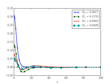
Figure 4. Profiles for the ground state and several excited states at $\gamma=1$. All have mass one.

6.2.4. Variable $E$ Profiles

Starting from the mass one profiles, we vary $E$ about the value computed above, and compute a collection of profiles for each of the nonlinear bound states. We plot the mass as a function of $E$ in Figure 5. Recall from the slope condition, (5.4), that since these appear to be strictly increasing in all cases, $p(d^{\prime\prime})=1$ in all of the cases we have computed. We speculate that this is true for all cases of this problem. The maximum value of $E$ at which we computed is, for each branch, twice the value of $E$ corresponding to the mass one problem. Each branch terminates at the corresponding eigenvalue of the associated linear problem.

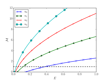
Figure 5. Mass as a function of $E$ for several branches of the problem. In all cases, the curves appear to be monotonically increasing.

6.2.5. Remarks

In our experience, this approach was highly robust. The continuation strategy from the linear problem to the nonlinear problem required a modest number of intermediate values of $\gamma$; $\delta\gamma=0.05$ was used in the above calculations. A slight difficulty occurs when considering states which branch from linear states with eigenvalues close to the origin. As mentioned earlier, while these will decay exponentially, the successively slower decay will require larger and larger domains.

6.3. Stability Calculations

To proceed with an analysis of the stability, we first need to discretize the operators, $L_{\pm}$, and then compute their eigenvalues.

6.3.1. Discretization of the Operators

To compute the spectrum of $L_{\pm}$, we continue to work within the FEM context. The one subtlety to this is how to represent the nonlocal linear operator, $(|x|^{-1}\ast(u\bullet))u$, in the weak form. Let $T$ denote this operator. We approximate it as follows. First note that the Galerkin weak form is

(6.13) $$\left\langle T\varphi_{i},\varphi_{j}\right\rangle=\langle u\underbrace{(|x|^{-1}\ast(u\varphi_{i}))}_{\equiv\psi^{(i)}},\varphi_{j}\rangle.$$

Observe that $\psi^{(i)}$ solves

(6.14) $$-\Delta\psi^{(i)}=u\varphi_{i},\quad\partial_{r}\psi^{(i)}(0)=0,\quad\lim_{r\to\infty}\psi^{(i)}(r)=0.$$

An artificial boundary condition is now needed to numerically solve this on our computational domain. First, we observe that since $\varphi_{i}$ have finite support and $u$ is highly localized, at large values of $r$, $-\varphi^{(i)}\approx 0$. Thus, we introduce the Robin condition at $r_{\max}$:

(6.15) $$\partial_{r}\psi^{(i)}(r_{\max})+\tfrac{1}{r_{\max}}\psi^{(i)}(r_{\max})=0.$$

The $\psi^{(i)}$ are then approximated in the space ${\rm span}(\varphi_{0},\ldots,\varphi_{n})$ by solving

(6.16) $$K_{\operatorname{Rob}}\boldsymbol{\psi}^{(i)}=U_{\operatorname{Mat}}\mathbf{e}_{i},$$

for $i=1,\ldots,n$. The matrix $U_{\operatorname{Mat}}$ is given by

(6.17) $$(U_{\operatorname{Mat}})_{ij}=\int u\varphi_{i}\varphi_{j}.$$

Note that $K_{\operatorname{Rob}}$ is an $n+1\times n+1$ matrix and $\boldsymbol{\psi}^{(i)}\in\mathbf{R}^{n+1}$. Here, we take $U_{\operatorname{Mat}}$ to be $n+1\times n+1$, with $i,j=0,\ldots,n$. Taking $\mathbf{e}_{i}\in\mathbf{R}^{n}$,

(6.18) $$\boldsymbol{\psi}^{(i)}=K_{\operatorname{Rob}}^{-1}U_{\operatorname{Mat}}I^{n+1,n}\mathbf{e}_{i},$$

where $I^{n+1,n}$ is an $n+1\times n$ matrix with ones along the main diagonal and zeros elsewhere. Thus,

(6.19) $$\begin{split}\left\langle T\varphi_{i},\varphi_{j}\right\rangle=\langle{u\psi^{(i)}}{\varphi_{j}}\rangle&\approx\sum_{k=0}^{n}\left\langle u\varphi_{k},\varphi_{j}\right\rangle(K_{\operatorname{Rob}}^{-1}U_{\operatorname{Mat}}I^{n+1,n}\mathbf{e}_{i})_{k}\\ &\quad=(U_{\operatorname{Mat}}K_{\operatorname{Rob}}^{-1}U_{\operatorname{Mat}}I^{n+1,n}\mathbf{e}_{i})_{j}\end{split}$$

Mapping back into the set of elements vanishing at $r_{\max}$, the weak form of $T$ corresponds to the matrix

(6.20) $$T_{\operatorname{Mat}}=I^{n,n+1}U_{\operatorname{Mat}}K_{\operatorname{Rob}}^{-1}U_{\operatorname{Mat}}I^{n+1,n}$$

Thus, the Galerkin FEM forms of the eigenvalue problems for $L_{\pm}$ are

(6.21a) $$L_{-}: (K_{\rm Dir}+EM_{\rm Dir}+U_{\operatorname{Mat}}){\bf v} =-\mu M_{\rm Dir}{\bf v},$$

(6.21b) $$L_{+}: (K_{\rm Dir}+EM_{\rm Dir}+U_{\operatorname{Mat}}-2T_{\operatorname{Mat}}){\bf v} =-\mu M_{\rm Dir}{\bf v}.$$

While it is intimidating to contend with the nonlocal operator, which, in discretized form, induces a dense matrix, we found that this was readily handled by SciPy, [13].

6.3.2. Eigenvalues of $L_{\pm}$

In Figure 6, we plot the numerically computed negative spectrum for the linearized operators. We note here that as described above for the full problem, the continuous spectrum for our linearized operators starts at $E>0$ and that infinitely many positive eigenvalues of the operators exist in between $0$ and $E$ due to the slow decay of the external potential. We note that under the assumptions that $L_{+}$ is invertible along the branch and using the nodal count for $L_{-}$ from the linear solutions, one can show that the number of negative eigenvalues for $L_{+}$ and $L_{-}$ does not change from that in the case of the linear problem, which is once again verified here numerically. We also see that the topological structure of the modes increases in a very similar fashion to that of the model Hydrogen atom problem. In the computed cases, for $E$ in excess of the zero mass limit, $L_{+}$ of $u_{j}$ has $j+1$ negative eigenvalues, while $L_{-}$ has $j$ eigenvalues. Thus, we always obtained $2j+1$ negative eigenvalues. This implies that the ground state is orbitally stable, since $n(L)=p(d^{\prime\prime})=1$. However, it is inconclusive for the excited states, since the difference between $n(L)$ and $p(d^{\prime\prime})=1$ is always a nonzero even number. These were computed using the mesh (6.5), with $r_{\max}=100$ and $n=2000$.

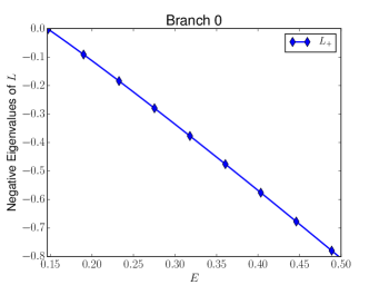
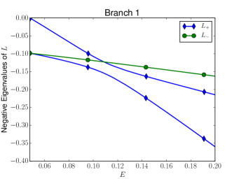
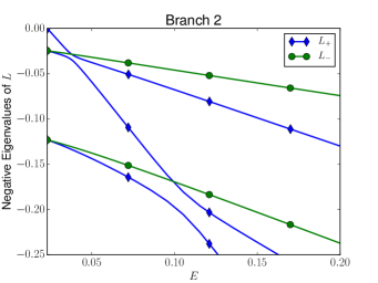
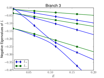
Figure 6. Numerically computed negative spectrum of $L_{\pm}$ for the ground state and the first three excited states. Notice the crossings of the spectral lines in amongst the excited states. These were computed on (6.5) with $r_{\max}=100$ and $n=2000$.

Remark.

Our key assumption is that the kernel of $L_{+}$ remains trivial along the branches we have constructed. This held in our numerical computations.

Since this is inconclusive, we instead discretize $JL$ directly, and examine its spectrum. For the first few states, this is plotted in Figure 7 for $E=1$ solutions. While the ground state has no linearly unstable states, each of the excited states has some number of linearly unstable modes, through the appearance of the quartets of point spectra. These were computed using the mesh (6.5), with $r_{\max}=100$ and $n=8000$. While we were able to use the automatically obtained mesh for computing the spectrum of just $L_{\pm}$, this resulted in spurious purely real eigenvalues which converged to the origin under mesh refinement. Indeed, in the case of the third branch, while not entirely visible, there is a pair of real eigenvalues with magnitude $\operatorname{O}(10^{-4})$. We believe these will tend to zero under further mesh refinement, which we were unable to do.

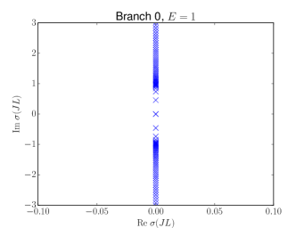
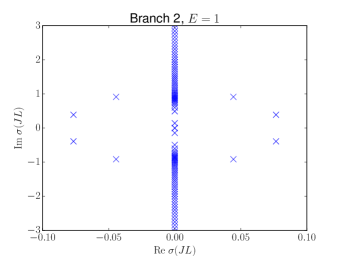
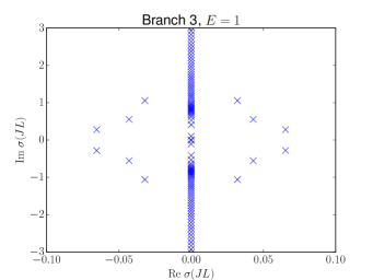
Figure 7. Numerically computed spectrum for $JL$ for the ground state and the first three excited states. Note the appearance of the quartets for the excited states implying linear instability. These were computed on (6.5) with $r_{\max}=100$ and $n=8000$.

6.3.3. Time-Dependent Simulations

To assess the stability of the nonlinear bound states, we resort to direct numerical simulation of

(6.22) $$i\partial_{t}\phi=-\Delta\phi+V(|x|)\phi-(-\Delta)^{-1}(\left|\phi\right|^{2})\phi$$

using perturbations of the solutions we computed in the previous section as initial conditions. Indeed, our data is of the form

(6.23) $$\phi_{0}=u_{j}(r)+\epsilon\exp\left\{-4(r-10)^{2}\right\}$$

with $\epsilon=10^{-4}$ and $u_{j}$ the $E=1$ solution of the $j$-th branch. We focus on the $E=1$ solutions, as these are highly localized, decaying $\propto e^{-r}$. Our results, pictured in Figure 8 show that while the ground state appears to be stable, the first excited state is unstable; this is consistent with our spectral computations. Throughout, we restrict to the radially symmetric problem, and solve the initial boundary value problem associated with (6.22) on $(0,r_{\max})$, with boundary conditions

(6.24) $$\partial_{r}\phi(0,t)=0,\quad\phi(r_{\max},t)=0.$$

We made use of the mesh (6.5).

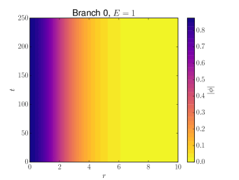
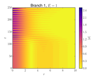
Figure 8. Time dependent simulations of the ground state and first excited state solutions with $E=1$, with perturbed initial condition (6.23).

Our algorithm is based on the Strang splitting method in [20]. We solve (6.22) through three successive problems. Given the solution at $t_{n}$, $\phi^{(n)}$,

(6.25) $$\phi^{\prime} =\exp\left\{\tfrac{i\Delta t}{2}(-\Delta)^{-1}|\phi^{{(n)}}|^{2}\right\}\phi^{{(n)}}$$

(6.26) $$\phi^{\prime\prime} =\left[I+\tfrac{i\Delta t}{2}(-\Delta+V)\right]^{-1}\left[I-\tfrac{i\Delta t}{2}(-\Delta+V)\right]\phi^{\prime}$$

(6.27) $$\phi^{(n+1)} =\exp\left\{\tfrac{i\Delta t}{2}(-\Delta)^{-1}|\phi^{\prime\prime}|^{2}\right\}\phi^{\prime\prime}$$

Problem (6.25) is accomplished by first solving

(6.28) $$-\Delta w=|\phi^{{(n)}}|^{2},\quad w^{\prime}(0)=0,\quad\lim_{r\to\infty}w(r)=0$$

on $(0,r_{\max})$ with radial piecewise linear finite elements and the Robin condition

$$w^{\prime}(r_{\max})+\tfrac{1}{r_{\max}}w(r_{\max})=0.$$

The FEM solution can be represented as

$${\bf w}=I^{n,n+1}K_{\operatorname{Rob}}^{-1}MI^{n+1,}|\boldsymbol{\phi}^{(n)}|^{2},$$

since $K_{\operatorname{Rob}}$ is an $n+1\times n+1$ matrix, due to the Robin condition, but our solution must satisfy the Dirichlet condition at $r_{\max}$. As before, $M$ is the mass matrix, and $K_{\operatorname{Rob}}$ is the stiffness matrix with Robin conditions. The nonlinearity is interpreted as an element-wise operation at the nodes. Once we have computed ${\bf w}$, we have

$$\boldsymbol{\phi}^{\prime}=\exp\left\{\tfrac{i\Delta t}{2}{\bf w}\right\}\boldsymbol{\phi}^{(n)},$$

where, again, the operation is element-wise on the nodes. Then, (6.26) is obtained from

(6.29) $$\boldsymbol{\phi}^{\prime\prime}=\left[M+\tfrac{i\Delta t}{2}K_{\operatorname{Dir}}+U_{\operatorname{Mat}}\right]^{-1}\left[M-\tfrac{i\Delta t}{2}K_{\operatorname{Dir}}+U_{\operatorname{Mat}}\right]\boldsymbol{\phi}^{\prime}.$$

Finally (6.27) is computed in the same way as (6.25). This method is efficient, as only sparse linear algebra operations are required, and accurate. The results shown in Figure 8 were obtained on the nonuniform mesh (6.5) with $r_{\max}=4000$, $\Delta t=0.00125$ and $n=64000$. They were stable to mesh refinement and other diagnostics.

To assess the accuracy of our simulations, we first examined the conservation of the invariants, numerically approximated by

(6.30) $$\mathcal{M}(\boldsymbol{\phi}) =\boldsymbol{\phi}^{T}M\boldsymbol{\phi},$$

(6.31) $$\mathcal{H}(\boldsymbol{\phi}) =\boldsymbol{\phi}^{T}(K_{\operatorname{Dir}}+U_{\operatorname{Mat}})\boldsymbol{\phi}-\tfrac{1}{2}(M|\boldsymbol{\phi}|^{2})^{T}K_{\operatorname{Rob}}^{-1}(M|\boldsymbol{\phi}|^{2}).$$

The results for the simulations corresponding to Figure 8 are shown in Figure 9. While the conservation of the ground state is excellent, there is a somewhat larger discrepancy with the first excited state, although the relative error over the lifetime of the simulation is still $\operatorname{O}(10^{-6})$. To verify that there was no error, we performed convergence testing, shown in Figure 10, indicating that the algorithm is converging under mesh refinement, and further accuracy could be gained with a reduction in $\Delta t$.

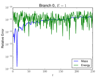
(a) Ground State

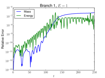
(b) First Excited State

Figure 9. Conservation of the numerical invariants under during the simulations. These are representative of our results and correspond to Figure 8.

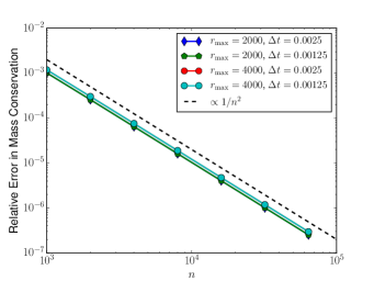
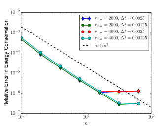
Figure 10. Convergence of the invariants for the time dependent simulations of the perturbed first excited state.

The only other comment we make on our methodology is that $r_{\max}$ must be sufficiently large to allow for the homogeneous Dirichlet condition at $r_{\max}$ in (6.24). While we used $r_{\max}=100$ to compute the nonlinear bound states, for the time-dependent problems we took $r_{\max}=2000$ and $r_{\max}=4000$. We thus matched the computed $u$ on $[0,100]$ to the far field asymptotics,

(6.32) $$u\sim Ke^{-\sqrt{E}r}r^{-1+\frac{1+m(100)}{2\sqrt{E}}},$$

to generate an initial condition.

In the time dependent simulations, the solution was typically smaller than $\operatorname{O}(10^{-8})$ at the boundary throughout the simulation when $r_{\max}=2000$ and smaller than $\operatorname{O}(10^{-15})$ when $r_{\max}=4000$. This, together with other convergence testing in time step, domain size, and mesh spacing leads us to believe that the stability and instability results we have observed are genuine and not numerical. They are also consistent with simulations appearing in [12], where the authors examined (1.1) in the setting $V=0$. There, they found the ground state to be stable and the first excited state to be unstable, agreeing with our simulations at $E=1$.

6.4. Transitions to Instability

While for $E=1$, the $JL$ spectral computations and time dependent simulations reveal linear instabilities of the excited state branches, the stability question for general $E$ remains unresolved. As Figure 11 shows, there may be some stable excited state solutions. In the figure, we have plotted the maximum of the real part of the $JL$ spectrum for a series of branch 1 excited states. These were computed using the nonuniform mesh with $r_{\max}=100$ and $n=2000$. Examining the figure, there appears to be a secondary bifurcation near $E=0.13$, where a linearly unstable eigenvalue first appears. Beneath that value, no such linear instability is present. With regard to bounds on unstable eigenvalues, we calculate in Appendix A that

(6.33) $$\sup\left|\mathrm{Re}\sigma(JL)\right|\leq C\|u_{E}\|_{L^{2}}^{2}\sqrt{\frac{1}{3}E+\frac{1}{3}\|V\|_{L^{\infty}}+\frac{2}{3}\|x\nabla V\|_{L^{\infty}}},$$

ensuring that unstable eigenvalues must vanish in the zero mass limit.

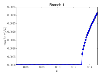
Figure 11. Numerically computed spectrum for $JL$ for the first excited state over a range of $E$ values, from the mass zero bifurcation value up to 0.15. Note the secondary bifurcation near $E=0.13$, where unstable eigenvalues appear. These correspond to quartets. when plotted in the complex plane. Computed on (6.5) with $r_{\max}=100$ and $n=2000$.

7. Discussion

We have analytically and numerically explored radial nonlinear bound state solutions of the Schrödinger-Poisson equation with an attractive Coulomb like potential. These states were shown to branch off of the discrete modes of the associated linear problem. Subject to a spectral assumption, these can be continued to have arbitrarily large mass and large $E$ parameter.

Our numerical methods for computing the solutions, first computing the linear modes, and then performing continuation in an artificial parameter, was robust. Subsequent time dependent simulations, using a FEM discretization and a splitting scheme, also proved themselves to be robust, showing excellent conservation of the invariants.

While our work implies the stability of the ground state at all values of $E$, we are unable to make any broad conclusions about the excited states. Our spectral and time dependent computations for the $E=1$ solutions imply they are linearly unstable. At the same time, in our examination of the $JL$ spectrum near the zero mass limit for branch 1, we see a subsequent bifurcation with the emergence of linearly unstable modes. Further investigation is necessary to explore the other states, and a spectral approach, such as the one used in [12] for $V=0$, may be of use. We also note the recent work [7], in which it is shown that the spectrally stable excited states can still be nonlinearly unstable through radiation damping and the Fermi Golden Rule, which require dispersive decay that is not understood for long range, Coulomb-style potentials.

In most applications, excited states can be both linearly unstable, as observed here for large enough $E$, as well as orbitally unstable due to radiation damping. For long range potentials of the case studied here, it is unknown how to quantify radiation effects. See, for instance, the work [28] for a discussion of resonant interactions and [14, 15, 22] in the setting of bifurcation theory for the excited state of a localized double well potential.

The promise of stable excited states in our setting is relevant given the observations in [3], that excess energy contained in a dwarf spheroidal galaxy corresponds to larger essential support of the dark matter field. By essential support here, we mean the volume of space on which the solution has non-trivial mass. This is contradictory to the nature of scaling of the ground state, which contracts its effective support as mass is increased in our model. Our numerics imply that for sufficiently large $E$, excited state branches are unstable. More refined numerical analysis and theory is required to determine if the conjecture of [3] about stability of excited state branches holds neared the bifurcation points. This merits future analytical and computational study.

Appendix A Bounds on Unstable Eigenvalues

To bound the positive real part of the eigenvalues of $JL$, we follow the results from [27] and [12, Appendix A]. First, we express the eigenvlaue problem as

(A.1) $$L_{-}v =\lambda u,$$

(A.2) $$L_{+}u =-\lambda v,$$

with

(A.3) $$L_{+}=L_{-}-2|x|^{-1}\ast(u_{E}\bullet)u_{E}.$$

Therefore

(A.4) $$\int\bar{u}L_{-}v-\int vL_{+}\bar{u}=\int\lambda|u|^{2}+\int\bar{\lambda}\bar{|v|^{2}}$$

Writing $\lambda=\sigma+i\tau$, and using the self adjointness of $L_{-}$,

(A.5) $$\sigma(\|u\|_{L^{2}}^{2}+\|v\|_{L^{2}}^{2})+i\tau(\|u\|_{L^{2}}^{2}-\|v\|_{L^{2}}^{2})=\int 2|x|^{-1}(u_{E}\bar{u})u_{E}v$$

Therefore, taking real parts and then absolute values,

(A.6) $$\begin{split}|\sigma|(\|u\|_{L^{2}}^{2}+\|v\|_{L^{2}}^{2})&=2\left|\mathrm{Re}\int|x|^{-1}(u_{E}\bar{u})u_{E}v\right|\\ &\leq 2\left|\int|x|^{-1}(u_{E}\bar{u})u_{E}v\right|\end{split}$$

By Hardy-Littlewood-Sobolev,

(A.7) $$\left|\int|x|^{-1}(u_{E}\bar{u})u_{E}v\right|\leq C_{\rm HLS}\|u_{E}u\|_{L^{6/5}}\|u_{E}v\|_{L^{6/5}}$$

By Hölder,

(A.8) $$\|u_{E}u\|_{L^{6/5}}\leq\|u_{E}\|_{L^{3}}\|u\|_{L^{2}}$$

Therefore,

(A.9) $$|\sigma|(\|u\|_{L^{2}}^{2}+\|v\|_{L^{2}}^{2})\leq 2C_{\rm HLS}\|u_{E}\|_{L^{3}}^{2}\|u\|_{L^{2}}\|v\|_{L^{2}}\leq C_{\rm HLS}\|u_{E}\|_{L^{3}}^{2}(\|u\|_{L^{2}}^{2}+\|v\|_{L^{2}}^{2})$$

Which gives our first bound:

(A.10) $$|\sigma|\leq C_{\rm HLS}\|u_{E}\|_{L^{3}}^{2}$$

We would like to have that as $E$ tends to the bifurcation value, $\|u_{E}\|_{L^{3}}$ tends to zero. By Hölder again, and Gagliardo-Nirenberg,

(A.11) $$\|u_{E}\|_{L^{3}}\leq\sqrt{\|u_{E}\|_{L^{6}}\|u_{E}\|_{L^{2}}}\leq\sqrt{C_{\rm GN}\|\nabla u_{E}\|_{L^{2}}\|u_{E}\|_{L^{2}}}$$

Therefore,

(A.12) $$|\sigma|\leq C_{\rm HLS}C_{\rm GN}\|\nabla u_{E}\|_{L^{2}}\|u_{E}\|_{L^{2}}$$

A bit more refinement can be done. To get further control in terms of $L^{2}$ norm alone, one can modify the energy-momentum tensor tensor techniques as applied in [27] and [12, Appendix A], to prove

(A.13) $$\int|\nabla u_{E}|^{2}dx=\frac{1}{3}E\int|u_{E}|^{2}dx-\frac{1}{3}\int V|u_{E}|^{2}+\frac{2}{3}\int x\cdot\nabla V|u_{E}|^{2}dx.$$

As a result, we have

(A.14) $$|\sigma|\leq C_{\rm HLS}C_{\rm GN}\|u_{E}\|_{L^{2}}^{2}\sqrt{\frac{1}{3}E+\frac{1}{3}\|V\|_{L^{\infty}}+\frac{2}{3}\|x\nabla V\|_{L^{\infty}}}$$

Thus we obtain a bound entirely in terms of $E$ and $\|u_{E}\|_{L^{2}}$.

To prove estimate (A.13), recall the energy-momentum tensor as applied in [27],

$$T_{ij} =\partial_{i}u_{E}\partial_{j}(\bar{u}_{E})+\partial_{j}u_{E}\partial_{i}(\bar{u}_{E})+\partial_{i}(|x|^{-1}*|u_{E}|^{2})\partial_{j}(|x|^{-1}*|u_{E}|^{2})$$

$$-\delta_{ij}\left(\sum_{k=1}^{3}(\partial_{k}u_{E}\partial_{k}(\bar{u}_{E})+\frac{1}{2}\partial_{k}(|x|^{-1}*|u_{E}|^{2})\partial_{k}(|x|^{-1}*|u_{E}|^{2}))\right.$$

$$\left.+\int V|u_{E}|^{2}dx-(|x|^{-1}*|u_{E}|^{2})|u_{E}|^{2}+E|u_{E}|^{2}\right).$$

This is identical up to the stress-energy tensor from [12, Appendix A] modulo terms with $V$. We claim that for $i=1,2,3$,

$$T_{ij,j}=\sum_{j=1}^{3}\partial_{j}(T_{ij})=-(\partial_{i}V).|u_{E}|^{2}$$

To see this, observe that

$$\frac{1}{2}\partial_{1}(|\partial_{1}u_{E}|^{2}-|\partial_{2}u_{E}|^{2}-|\partial_{3}u_{E}|^{2})+\partial_{2}(\partial_{1}u_{E}\partial_{2}\bar{u}_{E})+\partial_{3}(\partial_{1}u_{E}\partial_{3}\bar{u}_{E})$$

$$\hskip 56.9055pt=(\Delta\bar{u}_{E})\partial_{1}u_{E}.$$

For convenience, let us set $\phi=(x^{-1}\ast|u_{E}|^{2})$, the we have

$$T_{1j,j} =(\Delta\bar{u}_{E})\partial_{1}u_{E}+(\Delta u_{E})\partial_{1}\bar{u}_{E}+(\partial_{1}\phi)\Delta\phi-\partial_{1}(V|u_{E}|^{2}-\phi|u_{E}|^{2}+E|u_{E}|^{2})$$

$$=(V\bar{u}_{E}-\phi\bar{u}_{E}+E\bar{u}_{E})\partial_{1}u_{E}+(Vu_{E}-\phi u_{E}+Eu_{E})\partial_{1}\bar{u}_{E}-(\partial_{1}\phi)|u_{E}|^{2}$$

$$-\partial_{1}(V|u_{E}|^{2}-\phi|u_{E}|^{2}+E|u_{E}|^{2})$$

$$=-(\partial_{1}V)|u_{E}|^{2},$$

where we have used that $-\Delta\phi=|u_{E}|^{2}$. A similar calculation for $i=2,3$. Then,

$$\sum_{i=1}^{3}\sum_{j=1}^{3}\partial_{i}(T_{ij}x_{j})=\sum_{i=1}^{3}T_{ii}-(x\cdot\nabla V)|u_{E}|^{2}.$$

This implies

$$\int\sum_{i=1}^{3}T_{ii}dx-\int(x\cdot\nabla V)|u_{E}|^{2}dx=0,$$

and hence

$$0=\int\big{(}-|\nabla u_{E}|^{2}-\frac{1}{2}|\nabla\phi|^{2}+3\phi|u_{E}|^{2}-3V|u_{E}|^{2}$$

$$\hskip 56.9055pt-3E|u_{E}|^{2}-x\cdot\nabla V|u_{E}|^{2}\big{)}dx.$$

Recognizing that

$$\int|\nabla\phi|^{2}dx=-\int\Delta\phi\phi=-\int\phi|u_{E}|^{2}dx$$

and using that

$$-E\int|u_{E}|^{2}dx=\int|\nabla u_{E}|^{2}dx+\int V|u_{E}|^{2}dx-\int\phi|u_{E}|^{2}dx,$$

we arrive at (A.13).

References

- [1] Arnaud Anantharaman and Eric Cancès. Existence of minimizers for Kohn–Sham models in quantum chemistry. Annales de l’Institut Henri Poincare (C) Non Linear Analysis, 26(6):2425–2455, 2009.
- [2] R. Benguria, H. Brézis, and E. H. Lieb. The Thomas-Fermi-von Weizsäcker theory of atoms and molecules. Communications in Mathematical Physics, 79(2):167–180, 1981.
- [3] H.L. Bray. On dark matter, spiral galaxies, and the axioms of general relativity. Geometric Analysis, Mathematical Relativity, and Nonlinear Partial Differential Equations, 599:1–64, 2010.
- [4] H.L. Bray and A.S. Goetz. Wave Dark Matter and the Tully-Fisher Relation. arXiv:1409.7347, 2014.
- [5] H.L Bray and A.R. Parry. Modeling wave dark matter in dwarf spheroidal galaxies. In Journal of Physics: Conference Series, volume 615, page 012001. IOP Publishing, 2015.
- [6] Earl A Coddington and Norman Levinson. Theory of ordinary differential equations. Tata McGraw-Hill Education, 1955.
- [7] Scipio Cuccagna and Masaya Maeda. On orbital instability of spectrally stable vortices of the NLS in the plane. arXiv preprint arXiv:1508.03146, 2015.
- [8] M. Grillakis. Linearized instability for nonlinear schrödinger and Klein-Gordon equations. Communications on pure and applied mathematics, 41(6):747–774, 1988.
- [9] M. Grillakis. Analysis of the linearization around a critical point of an infinite dimensional Hamiltonian system. Communications on Pure and Applied Mathematics, 43(3):299–333, 1990.
- [10] M. Grillakis, J. Shatah, and W. Strauss. Stability theory of solitary waves in the presence of symmetry, i. Journal of Functional Analysis, 74(1):160–197, 1987.
- [11] S.J. Gustafson and I.M. Sigal. Mathematical concepts of quantum mechanics. Springer Science & Business Media, 2011.
- [12] Richard Harrison, Irene Moroz, and KP Tod. A numerical study of the Schrödinger–Newton equations. Nonlinearity, 16(1):101, 2002.
- [13] Eric Jones, Travis Oliphant, Pearu Peterson, et al. SciPy: Open source scientific tools for Python, 2001–. [Online; accessed 2016-04-20].
- [14] E. Kirr, P.G. Kevrekidis, and D.E. Pelinovsky. Symmetry-breaking bifurcation in the nonlinear Schrödinger equation with symmetric potentials. Communications in mathematical physics, 308(3):795–844, 2011.
- [15] E.W. Kirr, P.G. Kevrekidis, E. Shlizerman, and M.I. Weinstein. Symmetry-breaking bifurcation in nonlinear Schrödinger/Gross-Pitaevskii equations. SIAM Journal on Mathematical Analysis, 40(2):566–604, 2008.
- [16] R. Kollár and P.D. Miller. Graphical Krein Signature Theory and Evans–Krein Functions. SIAM Review, 56(1):73–123, 2014.
- [17] E. Lenzmann. Uniqueness of ground states for pseudorelativistic Hartree equations. Analysis & PDE, 2(1):1–27, 2009.
- [18] E.H. Lieb and B. Simon. The Hartree-Fock theory for Coulomb systems. Communications in Mathematical Physics, 53(3):185–194, 1977.
- [19] PL Lions. The choquard equation and related questions. Nonlinear Analysis: Theory, Methods & Applications, 4(6):1063–1072, 1980.
- [20] C. Lubich. On splitting methods for Schrödinger-Poisson and cubic nonlinear Schrödinger equations. Mathematics Of Computation, 77(264):2141–2153, 2008.
- [21] D. Olson, S. Shukla, G. Simpson, and D. Spirn. Petviashvilli’s Method for the Dirichlet Problem. Journal of Scientific Computing, pages 1–25, 2014.
- [22] DE Pelinovsky and TV Phan. Normal form for the symmetry-breaking bifurcation in the nonlinear schrödinger equation. Journal of Differential Equations, 253(10):2796–2824, 2012.
- [23] M. Reed and B. Simon. Analysis of Operators, Vol. IV of Methods of Modern Mathematical Physics. New York, Academic Press, 1978.
- [24] Hidetsugu Sakaguchi and Boris A Malomed. Suppression of quantum collapse in an anisotropic gas of dipolar bosons. Physical Review A, 84(3):033616, 2011.
- [25] Hidetsugu Sakaguchi and Boris A Malomed. Suppression of the quantum-mechanical collapse by repulsive interactions in a quantum gas. Physical Review A, 83(1):013607, 2011.
- [26] L.F. Shampine, P.H. Muir, and H. Xu. A User-Friendly Fortran BVP Solver. JNAIAM, 1(2):201–217, 2006.
- [27] KP Tod. The ground state energy of the Schrödinger–Newton equation. Physics Letters A, 280(4):173–176, 2001.
- [28] Tai-Peng Tsai and Horng-Tzer Yau. Relaxation of excited states in nonlinear schrödinger equations. International Mathematics Research Notices, 2002(31):1629–1673, 2002.
- [29] M.I. Weinstein. Modulational stability of ground states of nonlinear schrödinger equations. SIAM journal on mathematical analysis, 16(3):472–491, 1985.
- [30] M.I. Weinstein. Lyapunov stability of ground states of nonlinear dispersive evolution equations. Communications on Pure and Applied Mathematics, 39(1):51–67, 1986.