Recent progress in some exclusive and semi-exclusive processes in proton-proton collisions

Abstract

We present the main results of our recent analyses of exclusive production of vector charmonia ($J/\psi$ and $\psi^{\prime}$) in $k_{t}$-factorization approach and for $\gamma\gamma$ production of charged dilepton pairs in exclusive and semiinclusive processes in a new approach, similar in spirit to $k_{t}$-factorization.

The results for charmonia are compared with recent results of the LHCb collaboration. We include some helicity flip contributions and quantify the effect of absorption correction. The effect of $c\bar{c}$ wave function is illustrated.

We present uncertainties related to $F_{2}$ structure function which are the main ingredient of the approach. Our results are compared with recent CMS data for dilepton production with lepton isolation cuts imposed.

1 Introduction

Here we briefly summarize our recent results for exclusive production of $J/\psi$ mesons obtained in SS2007 ; CSS2015 and for photon-photon production of charged dileptons obtained in SFPSS2015 ; LSS2015 .

2 Exclusive production of vector charmonia

The Born diagrams for the exclusive production of $J/\psi$ mesons are shown in Fig.1. In actual calculations in SS2007 ; CSS2015 we include also absorption effects due to soft proton-proton interactions.

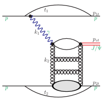
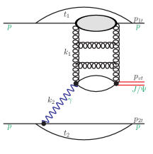
Figure 1: Born diagrams for exclusive production of $J/\psi$ mesons.

All details of the formalism can be found in Refs.SS2007 and CSS2015 . Here we only sketch the main points.

Imaginary part of the forward $\gamma p\to J/\psi p$ amplitude

$$\Im m\,{\cal M}_{T}(W,\Delta^{2}=0,Q^{2}=0)=W^{2}\frac{c_{v}\sqrt{4\pi\alpha_{em}}}{4\pi^{2}}\,2\,\int_{0}^{1}\frac{dz}{z(1-z)}\int_{0}^{\infty}\pi dk^{2}\psi_{V}(z,k^{2})$$

$$\int_{0}^{\infty}{\pi d\kappa^{2}\over\kappa^{4}}\alpha_{S}(q^{2}){\cal{F}}(x_{\rm eff},\kappa^{2})\Big{(}A_{0}(z,k^{2})\;W_{0}(k^{2},\kappa^{2})+A_{1}(z,k^{2})\;W_{1}(k^{2},\kappa^{2})\Big{)}\,.$$ (1)

The full amplitude, at finite momentum transfer is parametrized as:

$${\cal M}(W,\Delta^{2})=(i+\rho)\,\Im m{\cal M}(W,\Delta^{2}=0,Q^{2}=0)\,\exp(-B(W)\Delta^{2}/2)\,,$$ (2)

Then the amplitude for the $pp\to ppJ/\psi$ can be written somewhat formally as:

$${\cal M}_{h_{1}h_{2}\to h_{1}h_{2}V}^{\lambda_{1}\lambda_{2}\to\lambda^{\prime}_{1}\lambda^{\prime}_{2}\lambda_{V}}(s,s_{1},s_{2},t_{1},t_{2})={\cal M}_{\gamma{\bf I\!P}}+{\cal M}_{{\bf I\!P}\gamma}$$

$$=\langle{p_{1}^{\prime},\lambda_{1}^{\prime}}|J_{\mu}|{p_{1},\lambda_{1}}\rangle\epsilon_{\mu}^{*}(q_{1},\lambda_{V}){\sqrt{4\pi\alpha_{em}}\over t_{1}}{\cal M}_{\gamma^{*}h_{2}\to Vh_{2}}^{\lambda_{\gamma^{*}}\lambda_{2}\to\lambda_{V}\lambda_{2}}(s_{2},t_{2},Q_{1}^{2})$$

$$+\langle{p_{2}^{\prime},\lambda_{2}^{\prime}}|J_{\mu}|{p_{2},\lambda_{2}}\rangle\epsilon_{\mu}^{*}(q_{2},\lambda_{V}){\sqrt{4\pi\alpha_{em}}\over t_{2}}{\cal M}_{\gamma^{*}h_{1}\to Vh_{1}}^{\lambda_{\gamma^{*}}\lambda_{1}\to\lambda_{V}\lambda_{1}}(s_{1},t_{1},Q_{2}^{2})\,.$$ (3)

The auxiliary amplitude in Eq. (3) for the emission of a photon of transverse polarization $\lambda_{V}$, and transverse momentum $\mbox{\boldmath$q$}_{1}=-\mbox{\boldmath$p$}_{1}$ can be written as:

$$\langle{p_{1}^{\prime},\lambda_{1}^{\prime}}|J_{\mu}|{p_{1},\lambda_{1}}\rangle\epsilon_{\mu}^{*}(q_{1},\lambda_{V})={(\mbox{\boldmath$e$}^{*(\lambda_{V})}\mbox{\boldmath$q$}_{1})\over\sqrt{1-z_{1}}}\,{2\over z_{1}}\,\chi^{\dagger}_{\lambda^{\prime}}\Big{\{}F_{1}(Q_{1}^{2})-{i\kappa_{p}F_{2}(Q_{1}^{2})\over 2m_{p}}(\mbox{\boldmath$\sigma$}_{1}\cdot[\mbox{\boldmath$q$}_{1},\mbox{\boldmath$n$}])\Big{\}}\chi_{\lambda}\,.$$ (4)

Above $F_{1}$ and $F_{2}$ are Dirac and Pauli electromagnetic form factors, respectively. In Ref.CSS2015 we have included the Pauli form factors for a first time.

3 Selected results for vector quarkonia

Rapidity distributions of $J/\psi$ mesons are show in Fig.2. In this calculation Gaussian wave functions were used. Only results with UGDFs that include nonlinear effects describe the LHCb experimental distributions LHCb . In our opinion it is too preliminary to conclude that we observe nonlinear effects or onset of gluon saturation. In Ref.CSS2015 we obtained similar distributions for $\psi^{\prime}$ CSS2015 .

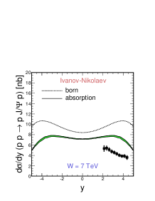
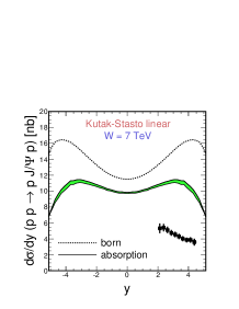
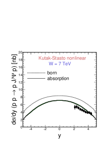
Figure 2: Rapidity distributions for three different unintegrated gluon distributions. The upper curves were obtained in the Born approximation and the lower band includes absorption effects.

Very interesting quantity is the ratio of the cross sections for $\psi^{\prime}$ and $J/\psi$ production. As shown in Fig.3 such a ratio is very sensitive to the functional form of the $c\bar{c}$ light-cone wave function. We conclude that the Gauss $c\bar{c}$ wave function much better describes the LHCb data LHCb than Coulomb WF. In some calculation in the literature the wave functions are not included explicitly and only point-like coupling is used Ryskin-Martin .

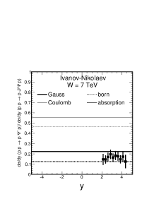
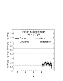
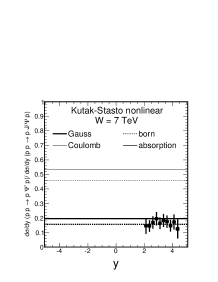
Figure 3: The ratio of the cross section for $\psi^{\prime}$ and $J/\psi$.

4 $\gamma\gamma$ production of dileptons

The $\gamma\gamma$ processes can be categorize according to the final state (see Fig.4). All the processes were discussed in SFPSS2015 ; LSS2015 .

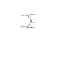
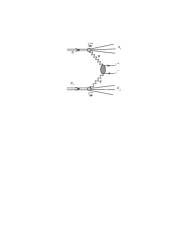
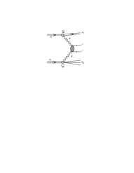
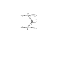
Figure 4: The different categories of $\gamma\gamma$ processes.

Two different approaches were discussed in the context of $\gamma\gamma$ production of dileptons.

In the collinear approach the corresponding cross sections are calculated respectively as:

$$\frac{d\sigma^{(k,l)}}{dy_{1}dy_{2}d^{2}p_{t}} = \frac{1}{16\pi^{2}{\hat{s}}^{2}}x_{1}\gamma_{k}(x_{1},\mu^{2})\;x_{2}\gamma_{l}(x_{2},\mu^{2})\;\overline{|{\cal M}_{\gamma\gamma\to l^{+}l^{-}}|^{2}}\,,$$ (5)

where $k,l\in\{\rm{el},\rm{in}\}$ stand for the processes with intact ($\rm{el}$) or dissociated $\rm{in}$ proton at the photon vertex. The $\gamma_{k}(x,\mu^{2})$ are the corresponding photon distributions in a proton, with or without the condition of breakup. The elastic photon distributions are calculated with the help of the nucleon electromagnetic form factors, while the inelastic distributions can be obtained by using a combined QCD/QED evolution QED-PDF .

In the $k_{t}$-factorization, proposed recently in SFPSS2015 ; LSS2015 , the fully unintegrated photon flux can be written as (below incoming particles are denoted as $A,B$):

$${d{\cal{F}}_{\gamma^{*}\leftarrow A}(z,\mbox{\boldmath$q$},M_{X}^{2})\over dM_{X}^{2}}={\alpha_{\rm{em}}\over\pi}\,(1-z)\,\Big{(}{\mbox{\boldmath$q$}^{2}\over\mbox{\boldmath$q$}^{2}+z(M_{X}^{2}-m_{A}^{2})+z^{2}m_{A}^{2}}\Big{)}^{2}\,\cdot{p_{B}^{\mu}p_{B}^{\nu}\over s^{2}}\,W_{\mu\nu}(M_{X}^{2},Q^{2})\,.$$ (6)

Information on the virtual photon-proton interaction is contained in the hadronic tensor, which is obtained in terms of the electromagnetic currents as:

$$W_{\mu\nu}(M_{X}^{2},Q^{2})=\overline{\sum_{X}}(2\pi)^{3}\,\delta^{(4)}(p_{X}-p_{A}-q)\,\langle{p}|J_{\mu}|{X}\rangle\langle{X}|J_{\nu}^{\dagger}|{p}\rangle\,d\Phi_{X}\,,$$ (7)

The virtual photoabsorption cross sections are related to hadronic tensors as:

$$\sigma_{T}(\gamma^{*}p)={4\pi\alpha_{em}\over 4\sqrt{X}}\,\Big{(}-{\delta^{\perp}_{\mu\nu}\over 2}\Big{)}2\pi W^{\mu\nu}(M_{X}^{2},Q^{2})\,,\,\sigma_{L}(\gamma^{*}p)={4\pi\alpha_{em}\over 4\sqrt{X}}\,e^{0}_{\mu}e^{0}_{\nu}\,2\pi W^{\mu\nu}(M_{X}^{2},Q^{2})\,.$$ (8)

It is customary to introduce dimensionless structure function $F_{i}(x_{\rm Bj},Q^{2}),i=T,L$ as

$$\sigma_{T,L}(\gamma^{*}p)={4\pi^{2}\alpha_{em}\over Q^{2}}\,{1\over\sqrt{1+{4x^{2}_{\rm Bj}m_{A}^{2}\over Q^{2}}}}\,F_{T,L}(x_{\rm Bj},Q^{2})\,,$$ (9)

At high energies, in the calculation of photon fluxes, the contribution of the structure function

$$F_{2}(x_{\rm Bj},Q^{2}) = {F_{T}(x_{\rm Bj},Q^{2})+F_{L}(x_{\rm Bj},Q^{2})\over 1+{4x^{2}_{\rm Bj}m_{A}^{2}\over Q^{2}}}$$ (10)

dominates.

The unintegrated fluxes enter the cross section for dilepton production as

$${d\sigma^{(i,j)}\over dy_{1}dy_{2}d^{2}\mbox{\boldmath$p$}_{1}d^{2}\mbox{\boldmath$p$}_{2}} =\int{d^{2}\mbox{\boldmath$q$}_{1}\over\pi\mbox{\boldmath$q$}_{1}^{2}}{d^{2}\mbox{\boldmath$q$}_{2}\over\pi\mbox{\boldmath$q$}_{2}^{2}}{\cal{F}}^{(i)}_{\gamma^{*}/A}(x_{1},\mbox{\boldmath$q$}_{1})\,{\cal{F}}^{(j)}_{\gamma^{*}/B}(x_{2},\mbox{\boldmath$q$}_{2}){d\sigma^{*}(p_{1},p_{2};\mbox{\boldmath$q$}_{1},\mbox{\boldmath$q$}_{2})\over dy_{1}dy_{2}d^{2}\mbox{\boldmath$p$}_{1}d^{2}\mbox{\boldmath$p$}_{2}}\,,$$ (11)

where $i,j\in\{\rm{el},\rm{in}\}$ again refer to elastic and inelastic processes on the proton sides. For brevity we integrated over invariant masses of the possible dissociated system.

The longitudinal momentum fractions carried by photons can be obtained from rapidities and transverse momenta of the charged leptons as:

$$x_{1}=\sqrt{{\mbox{\boldmath$p$}_{1}^{2}+m_{l}^{2}\over s}}e^{y_{1}}+\sqrt{{\mbox{\boldmath$p$}_{2}^{2}+m_{l}^{2}\over s}}e^{y_{2}}\;,x_{2}=\sqrt{{\mbox{\boldmath$p$}_{1}^{2}+m_{l}^{2}\over s}}e^{-y_{1}}+\sqrt{{\mbox{\boldmath$p$}_{2}^{2}+m_{l}^{2}\over s}}e^{-y_{2}}\,.$$ (12)

5 Selected results for $l^{+}l^{-}$ production

As an example in Fig.5 we show invariant mass distributions for double dissociative processes (both protons undergo electromagnetic dissociation). The calculations have been performed for different experimental conditions specified in the figure legend. We show results for different proton structure functions from the literature. The different structure functions lead to quite different results. The presented results strongly depend on the kinematical regions of longitudinal momentum fraction and photon virtuality ($x$,$Q^{2}$) which were not sufficiently well studied experimentally and theoretically in which an interplay of perturbative and nonperturbative effects takes place. We observe that the $\gamma\gamma$ contribution constitutes only a small fraction of the cross section compared to the experimental data and Drell-Yan contribution (not shown explicitly here). Similar results for elastic-inelastic channel were shown in LSS2015 .

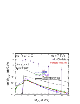
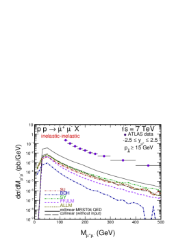
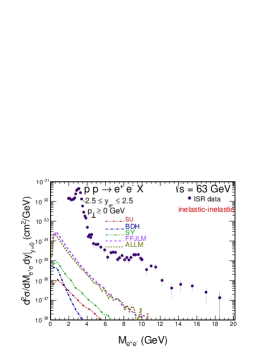
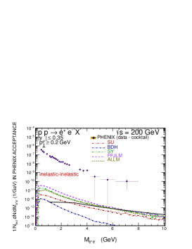
Figure 5: Dilepton invariant mass distributions for different experimental conditions (see the four panels) and for different structure functions (see different lines).

Now we wish to show results which can be directly compared to experimental data CMS . The data were obtained by imposing a kinematical constraint on lepton isolation. The results are shown in Figs.6,7, 8. A relatively good agreement has been achieved. A better quality results are expected from Run II at the LHC.

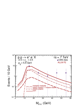
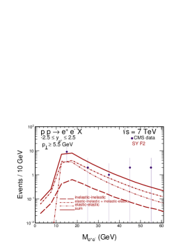
Figure 6: Dilepton invariant mass distributions for two (best) structure functions. The CMS data points are shown for comparison.

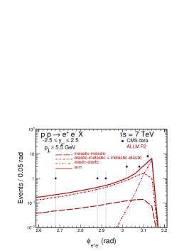
Figure 7: Distribution in relative azimuthal angle between leptons for two (best) structure functions. The CMS data points are shown for comparison.

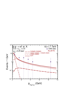
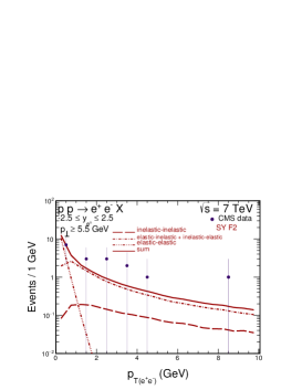
Figure 8: Distribution in transverse momentum of the pair of leptons for two (best) structure functions. The CMS data points are shown for comparison.

6 Conclusions

Our results and open problems for charmonia production can be summarized as follows. We have found some model dependent indication of presence of nonlinear effects in the small-$x$ gluon distribution of a proton. It is important to remember, that the present experiments are not fully exclusive and rather semi-inclusive processes have to be studied. Experimentally so far proton dissociation has been "extracted" in a model dependent way assuming some functional form in $p_{t}$. From HERA we have some limited knowledge only about diffractive dissociation. Compared to exclusive production of $J/\psi$ at HERA, in $pp$ collisions there is also electromagnetic dissociation. Interference effects due to the two diagrams in Fig. 1 were predicted. It would be nice to see a modulation in $\phi_{pp}$ due to interference effects between the two diagrams. In the future, the CMS+TOTEM and ATLAS+ALFA experiments could measure purely exclusive reaction and study dependence on many more variables.

Our results for photon-photon induced processes can be summarized as: We discussed two different approaches for $\gamma\gamma$ processes – collinear and $k_{t}$-factorization, they are not completely equivalent. We have found strong dependence on the structure function input to the photon fluxes in the $k_{t}$-factorization approach. Semi-exclusive contributions with dissociation are large which is an interesting lesson for $pp\to ppJ/\psi$. The photon-photon contributions are, however, rather small compared to the Drell-Yan contribution. A reasonable description of the CMS data with isolated electrons was obtained (recently also the ATLAS collaboration obtained similar results). So far only the collinear approach has been applied e.g. to the $pp\to(\gamma\gamma)\to W^{+}W^{-}XY$ processes. Such a reaction is important in searches for Beyond Standard Model effects. A large cross section was found LSR2015 . A calculation in $k_{t}$-factorization approach would be very valuable.

References

• (1) W. Schäfer and A. Szczurek, Phys. Rev. D76 (2007) 094014.
• (2) A. Cisek, W. Schäfer and A. Szczurek, JHEP 1504 (2015) 159,
• (3) R. Aaij et al. [LHCb Collaboration], J. Phys. G 40 (2013) 045001 [arXiv:1301.7084 [hep-ex]]; R. Aaij et al. [LHCb Collaboration], J. Phys. G 41 (2014) 055002 [arXiv:1401.3288 [hep-ex]].
• (4) S. P. Jones, A. D. Martin, M. G. Ryskin and T. Teubner, JHEP 1311 (2013) 085 [arXiv:1307.7099].
• (5) M. Łuszczak, W. Schäfer and A. Szczurek, arXiv:1510.00294,
• (6) G. Gil da Silveira, L. Forthomme, K. Piotrzkowski, W. Schäfer, A. Szczurek, JHEP 1502 (2015) 159,
• (7) A. D. Martin, R. G. Roberts, W. J. Stirling and R. S. Thorne, Eur. Phys. J. C 39, 155 (2005) [hep-ph/0411040].
• (8) S. Chatrchyan et al. [CMS Collaboration], JHEP 1211, 080 (2012) [arXiv:1209.1666 [hep-ex]].
• (9) M. Łuszczak, A. Szczurek and C. Royon, JHEP 1502 (2015) 098 [arXiv:1409.1803 [hep-ph]].