Singularities of solutions to quadratic vector equations on complex upper half-plane

Abstract

Let $S$ be a positivity preserving symmetric linear operator acting on bounded functions. The nonlinear equation $-\frac{1}{m}=z+Sm$ with a parameter $z$ in the complex upper half-plane $\mathbb{H}$ has a unique solution $m$ with values in $\mathbb{H}$. We show that the $z$-dependence of this solution can be represented as the Stieltjes transforms of a family of probability measures $v$ on $\mathbb{R}$. Under suitable conditions on $S$, we show that $v$ has a real analytic density apart from finitely many algebraic singularities of degree at most three.

Our motivation comes from large random matrices. The solution $m$ determines the density of eigenvalues of two prominent matrix ensembles; (i) matrices with centered independent entries whose variances are given by $S$ and (ii) matrices with correlated entries with a translation invariant correlation structure. Our analysis shows that the limiting eigenvalue density has only square root singularities or a cubic root cusps; no other singularities occur.

Keywords: Stieltjes-transform, Algebraic singularity, Density of states, Cubic cusp
AMS Subject Classification (2010): 45Gxx, 46Txx, 60B20, 15B52.

1 Introduction

Given a symmetric $N\times N$-matrix $S=(s_{ij})_{i,j=1}^{N}$ with non-negative entries and a complex number $z$ in the upper half-plane $\mathbb{H}:=\{z\in\mathbb{C}:\,\mathrm{Im}\,z\,>\,0\}$, we consider the system of $N$ non-linear equations

$$-\,\frac{1}{m_{i}\!}\;=\;z\,+\,\sum_{j=1}^{N}s_{ij}\mspace{1.0mu}m_{j}\,,\qquad i=1,\dots,N\,,$$ (1.1)

for $N$ unknowns $m_{1},\dots,m_{N}\in\mathbb{H}$. This is one of the simplest nonlinear systems of equations involving a general linear part. We will consider a general version of this problem, where $S$ is replaced by a linear operator acting on the Banach space of $\mathbb{H}$-valued bounded functions $m$ on some measure space that replaces the underlying discrete space of $N$ elements in (1.1).

In this paper we give a detailed analysis of the singularities of the solution of (1.1) as a function of the parameter $z$. In particular, we show that $m(z)$ is analytic in $z$ down to the real axis, apart from a few singular points. Our main result, Theorem 2.6, asserts that, under some natural conditions on $S$, these singularities are algebraic and they can be of degree two or three only. In fact, the components of $m(z)$ are the Stieltjes transforms of a family of densities on $\mathbb{R}$ with a common support consisting of finitely many compact intervals. The singularities of $m(z)$ originate from the behavior of these densities at the points where they vanish. We show that the densities are real analytic whenever they are positive and that they can only have square root singularities at the boundary (edges) of their support and cubic root cusps inside the interior.

Looking at (1.1) directly, the solutions of this system of $N$ quadratic equations in $N$ variables are algebraic functions of large degree in $z$. Thus, algebraic singularities of very high order are theoretically possible and in case of an infinite dimensional Banach space apparently even non-algebraic singularities might emerge. Our result excludes these scenarios and precisely classifies the possible singularities.

The system of equations (1.1) naturally appears in the spectral analysis of large random matrices and other related problems. It has been analysed in this context by many authors; e.g. Berezin [10], Wegner [40], Girko [23], Khorunzhy and Pastur [28], see also the more recent papers [7, 24, 37]. We mention two prominent examples in this direction.

The first example is a Wigner-type matrix with a general variance structure (Section 3.1). Let $H=(h_{ij})_{i,j=1}^{N}$ be an $N\times N$ real symmetric or complex hermitian matrix with centered entries and variance matrix $S$, i.e., $\mathbb{E}\,h_{ij}=0$, $\mathbb{E}\mspace{2.0mu}|h_{ij}|^{2}=s_{ij}$. The matrix elements are independent up to the symmetry constraint, $h_{ji}=\overline{h}_{ij}$. Let $G(z)=(H-z)^{-1}$ be the resolvent of $H$ with a spectral parameter $z\in\mathbb{H}$ and matrix elements $g_{ij}=g_{ij}(z)$. Second order perturbation theory indicates that

$$-\frac{1}{g_{ii}\!}\,\approx\,z+\sum_{j=1}^{N}s_{ij}\mspace{1.0mu}g_{j\mspace{-1.0mu}j}\,,$$ (1.2)

(see [19] in the special case when the sums $\sum_{j}s_{ij}$ are independent of $i$). In particular, if (1.1) is stable under small perturbations, then $g_{ii}$ is close to $m_{i}$ and the average $N^{-1}\sum_{i}m_{i}$ approximates the normalized trace of the resolvent, $N^{-1}\mathrm{Tr}\,G$. Being determined by $N^{-1}\mathrm{Im}\,\mathrm{Tr}\,G$, as $\mathrm{Im}\,z\to 0$, the empirical spectral measure of $H$ approaches the non-random measure with density

$$\rho(\tau)\,:=\,\lim_{\eta\mspace{1.0mu}\downarrow\mspace{1.0mu}0}\frac{1}{\pi\mspace{1.0mu}N}\sum_{i=1}^{N}\mathrm{Im}\,m_{i}(\tau+\mathrm{i}\mspace{1.0mu}\eta)\,,\qquad\tau\in\mathbb{R}\,,$$ (1.3)

as $N$ goes to infinity, see [8, 24, 37].

In the second example, we consider a random matrix of the form ${H}={X}+{X}^{*}$ where ${X}$ has correlated entries with a translation invariant correlation structure. As the dimension of ${H}$ grows, its empirical spectral measure approaches [3, 9, 15, 28, 35] a non-random measure with density $\rho$ defined through (1.3). In this setup $m_{i}$ solves (1.1) with $s_{ij}$ given by the Fourier transform of the correlation matrix (see Section 3.3).

Apart from a few specific cases, solving (1.1) and then computing $\rho(\tau)$ via (1.3) is the only known effective way to determine the spectral density of these large random matrices. Similarly, the limiting density, as $N\to\infty$, is computed by solving a continuous (integral) version of (1.1). Since much numerical and theoretical research [25, 36, 38] focuses on the density, it is somewhat surprising that no detailed analytical study of (1.1) has been initiated so far which goes beyond establishing existence, uniqueness, and regularity in the regime where the parameter $z$ is away from the real axis [1, 23, 26, 35]. Typically, the limiting density is compactly supported on a few disjoint intervals. Numerical studies [14, 20, 29, 31, 36] indicate that generically the limiting density exhibits square root singularities at the edges of these intervals. However, prior to the current work this finding has never been rigorously confirmed apart from a few explicitly computable cases [25, 36, 38]. Even less has been known about the possible formation of other singularities [36]. In a special Gaussian model the cubic singularity has been shown to emerge [13] as a gap in the support of the density closes. For random matrices with translation invariant correlation structure Theorem 2.4 of [7] shows that also the Stieltjes transform $m(z)$ of the limiting density satisfies a polynomial equation of the form $P(\mspace{1.0mu}z\mspace{1.0mu},m(z))=0$, but the degree of $P$ is unspecified. Our result applies to the setup of [7] and limits the algebraic singularities to degrees two or three (Section 3.4).

We remark that for invariant random matrix ensembles with a real analytic potential the singularities of the density have been classified [16, 30, 34]. In the generic case the singularities at the edges of the support of the density are also of square root type. For specific potentials the density may vanish at half-integer powers at the edges and any even power in the interior of the support but, in contrast to our result, cubic root cusp singularities do not occur for these ensembles.

So far we discussed qualitative properties of the spectral density on the macroscopic scale but the significance of (1.1) goes well beyond that. First, the algebraic order of the singularity of the limiting density at the edges predicts the typical scale of fluctuation of the extreme eigenvalues. Second, the recent proofs of the Wigner-Dyson-Mehta conjecture on the universality of local eigenvalue statistics heavily rely on understanding the spectral density on very small scales (see [18] for a complete history). One key ingredient to obtain such a local law is a very accurate stability analysis of the equation that determines the spectral density, here (1.1). The stability deteriorates near the singularities and extracting the necessary information requires a thorough quantitative analysis of $m$ at these points.

Our project has three main parts. In the current paper we present general qualitative results on the singularities of (1.1). We believe that this analysis is of interest in its own right since (1.1) appears in other contexts as well, even beyond random matrices [12, 27, 40]. The quantitative description of the singularities together with the stability analysis, tailored to the specific needs to prove the local law, will be presented in details in [4]. Finally, the local law and spectral universality for the corresponding random matrices will be proved in [5] with a separate discussion of the correlated case in [3]. The current paper is self-contained and random matrices will not appear here; they were mentioned only to motivate the problem.

2 Main result

For a measurable space $\mathfrak{A}$ and a subset $\mathbb{D}\subseteq{\mathbb{C}}$ of the complex numbers, we denote by $\mathcal{B}(\mathfrak{A},\mathbb{D})$ the space of bounded measurable functions on $\mathfrak{A}$ with values in $\mathbb{D}$. Let $(\mathfrak{X},\pi(\mathrm{d}x))$ be a measure space with bounded positive (non-zero) measure $\pi$. Suppose we are given a real valued function $a\in\mathcal{B}(\mathfrak{X},\mathbb{R})$ and a non-negative, symmetric, $s_{xy}=s_{yx}$, function $s\in\mathcal{B}(\mathfrak{X}^{2},\mathbb{R}_{0}^{+})$. Then we consider the quadratic vector equation (QVE),

$$-\frac{1}{m(z)}\,=\,z+a+Sm(z)\,,\qquad z\in\mathbb{H}\,,$$ (2.1)

for a function $m:\mathbb{H}\to\mathcal{B}(\mathfrak{X},\mathbb{H}),\,z\mapsto m(z)$, where $S:\mathcal{B}(\mathfrak{X},{\mathbb{C}})\to\mathcal{B}(\mathfrak{X},{\mathbb{C}})$ is the integral operator with kernel $s$,

$$(Sw)_{x}\,:=\,\int s_{xy}\mspace{1.0mu}w_{y}\mspace{1.0mu}\pi(\mathrm{d}y)\,,\qquad x\in\mathfrak{X}\,,\;w\in\mathcal{B}(\mathfrak{X},{\mathbb{C}})\,.$$

We equip the space $\mathcal{B}(\mathfrak{X},{\mathbb{C}})$ with its natural norm,

$$\lVert w\rVert\,:=\,\sup_{x\mspace{1.0mu}\in\mspace{1.0mu}\mathfrak{X}}\mspace{2.0mu}\lvert w_{x}\rvert\,,\qquad w\in\mathcal{B}(\mathfrak{X},{\mathbb{C}})\,.$$

With this norm $\mathcal{B}(\mathfrak{X},{\mathbb{C}})$ is a Banach space. For an operator $T$ on $\mathcal{B}(\mathfrak{X},{\mathbb{C}})$ we write $\lVert T\rVert$ for the induced operator norm.

The following result is considered folklore in the literature (see e.g. [8, 23, 26, 27, 28]). For completeness we include its proof, adjusted to our setup, in the Appendix A.

Proposition 2.1 (Existence and uniqueness).

The QVE has a unique solution $m$. For each $x\in\mathfrak{X}$ there exists a unique probability measure $v_{x}(\mathrm{d}\tau)$ on $\mathbb{R}$ such that

$$m_{x}(z)\,=\,\int_{\mathbb{R}}\frac{\mspace{1.0mu}v_{x}(\mathrm{d}\tau)\!}{\tau\mspace{1.0mu}-\mspace{1.0mu}z}\,,\qquad z\in\mathbb{H}\,.$$ (2.2)

All these measures have support in the compact interval $[-\kappa,\kappa]$ with

$$\kappa\,:=\,\lVert a\rVert+2\mspace{1.0mu}\lVert S\rVert^{1/2}.$$ (2.3)

The family $(v_{x})_{x\in\mathfrak{X}}$ constitutes a measurable function $v:\mathfrak{X}\to\mathcal{M}(\mathbb{R}),\;x\mapsto v_{x}$, where $\mathcal{M}(\mathbb{R})$ denotes the space of probability measures on $\mathbb{R}$ equipped with the weak topology.

Since by (2.2) the measure $v_{x}$ determines the component $m_{x}$ of the solution to the QVE, we consider this measure as a fundamental quantity and often express properties of $m$ in terms of properties of $v$.

Definition 2.2 (Generating measure).

The family of probability measures $v=(v_{x})_{x\in\mathfrak{X}}$, uniquely defined by the relation (2.2), is called the generating measure of the QVE. In case all measures $v_{x}$ admit a bounded Lebesgue-density, $v_{x}(\mathrm{d}\tau)=v_{x}(\tau)\mathrm{d}\tau$, the (almost everywhere defined) function $v:\mathbb{R}\to\mathcal{B}(\mathfrak{X},\mathbb{R}_{0}^{+}),\,\tau\mapsto v(\tau)$ is called the generating density of the QVE.

By a trivial rescaling we may from now on assume that $\pi$ is a probability measure, $\pi(\mathbb{R})=1$. We introduce a short notation for the average of a function on $\mathfrak{X}$ with respect to this measure

$$\langle\mspace{1.0mu}w\mspace{1.0mu}\rangle\,:=\,\int w_{x}\mspace{1.0mu}\pi(\mathrm{d}x)\,,\qquad w\in\mathcal{B}(\mathfrak{X},{\mathbb{C}})\,.$$

We need three assumptions on the data $a$ and $s$ of the QVE.

1. Diagonal positivity: There exists a symmetric, $r_{yx}=r_{xy}$, function $r\in\mathcal{B}(\mathfrak{X}^{2},\mathbb{R}_{0}^{+})$ such that

   $$s_{xy}\,\geq\,\int r_{xu}\mspace{1.0mu}r_{uy}\mspace{1.0mu}\pi(\mathrm{d}u)\,,\qquad x,y\in\mathfrak{X}\,,$$ (2.4)

   and $\inf_{x\in\mathfrak{X}}\int r_{xy}\mspace{1.0mu}\pi(\mathrm{d}y)>0$.

2. Uniform primitivity: There is some $K\in{\mathbb{N}}$ such that

   $$\inf_{x,y\in\mathfrak{X}}s^{(K)}_{xy}\,>\,0\,,$$ (2.5)

   where $s^{(K)}\in\mathcal{B}(\mathfrak{X}^{2},\mathbb{R}_{0}^{+})$ is the integral kernel of the $K$-th power $S^{\mspace{1.0mu}K}$ of the operator $S$.

3. Component regularity: There are no outlier components in the sense that

   $$\lim_{\varepsilon\downarrow 0}\inf_{x\in\mathfrak{X}}\int\frac{\pi(\mathrm{d}y)}{\varepsilon+(a_{x}-a_{y})^{2}+\langle\mspace{1.0mu}(S_{x}-S_{y})^{2}\rangle}\,=\,\infty\,,$$ (2.6)

   where $S_{x}:=(y\mapsto s_{xy})\in\mathcal{B}(\mathfrak{X},\mathbb{R}_{0}^{+})$ for each $x\in\mathfrak{X}$ denotes the $x$-th component of $S$.

In the following remarks we mention a few examples that illustrate the meaning of the assumptions (A), (B) and (C). The statements of these remarks are easy to check.

Remark 2.3.

If $\mathfrak{X}$ is equipped with a metric $d_{\mathfrak{X}}$ and $s$ has a positive strip along the diagonal in the sense that

$$s_{xy}\,\geq\,c\mspace{1.0mu}\mathbbm{1}(d_{\mathfrak{X}}(x,y)\leq\varepsilon)\,,\qquad x,y\in\mathfrak{X}\,,$$

for some positive constants $c$ and $\varepsilon$, then (2.4) is satisfied with the choice

$$r_{xy}\,:=\,c^{1/2}\mathbbm{1}(d_{\mathfrak{X}}(x,y)\leq\varepsilon/2)\,,\qquad x,y\in\mathfrak{X}\,.$$

Remark 2.4.

If $\mathfrak{X}$ admits a finite measurable partition, $\mathfrak{I}_{1},\dots,\mathfrak{I}_{n}$, such that each $\mathfrak{I}_{i}$ has positive measure and there is a primitive matrix $P=(p_{ij})_{i,j=1}^{n}\in\mathbb{R}^{n\times n}$ such that $s$ satisfies

$$s_{xy}\,\geq\,\sum_{i,j=1}^{n}p_{ij}\mathbbm{1}(x\in\mathfrak{I}_{i}\mspace{1.0mu},\mspace{2.0mu}y\in\mathfrak{I}_{j})\,,\qquad x,y\in\mathfrak{X}\,,$$

then (B) holds. Recall that a matrix $P$ is called primitive, if it has non-negative entries and there exists $k\in{\mathbb{N}}$ such that all entries of $P^{k}$ are strictly positive. If, additionally, the matrix $P$ has a positive diagonal, $p_{ii}>0$, then assumption (A) is satisfied as well.

Remark 2.5.

Assumption (C) is trivially satisfied if $\mathfrak{X}$ is finite and every $x\in\mathfrak{X}$ has positive measure. The integral in (2.6) provides a way to measure the regularity of $s$ and $a$ as the following example indicates. Consider the setup $(\mathfrak{X},\pi(\mathrm{d}x))=([0,1],\mathrm{d}x)$ and let $I_{1},\dots,I_{n}$ be a partition of $[0,1]$ into finitely many non-trivial intervals. Suppose $a$ and $s$ are piecewise $1/2$-Hölder continuous,

$$\sup_{x,\mspace{1.0mu}y\mspace{1.0mu}\in\mspace{1.0mu}I_{i}}\frac{\lvert a_{x}-a_{y}\rvert}{\mspace{10.0mu}\lvert x-y\rvert^{1/2}\mspace{-5.0mu}}\,<\,\infty\,,\quad\sup_{\genfrac{}{}{0.0pt}{1}{x_{1},\mspace{2.0mu}x_{2}\in I_{i}}{y_{1},\mspace{2.0mu}y_{2}\in I_{j}}}\frac{\lvert s_{x_{1}y_{1}}-s_{x_{2}y_{2}}\rvert}{\lvert x_{1}-x_{2}\rvert^{1/2}+\lvert y_{1}-y_{2}\rvert^{1/2}}\,<\,\infty\,,$$ (2.7)

for all $i,j=1,\dots,n$. Then (C) is satisfied.

Now we state our main theorem.

Theorem 2.6 (Regularity and singularities of the generating density).

Suppose $s$ and $a$ satisfy the assumptions (A), (B) and (C). Then the generating measure has a Lebegue-density $v_{x}(\mathrm{d}\tau)=v_{x}(\tau)\mathrm{d}\tau$ and this density is uniformly $1/3$-Hölder continuous

$$\sup_{x\in\mathfrak{X}}\sup_{\tau_{1}\neq\tau_{2}}\frac{\lvert\mspace{1.0mu}v_{x}(\tau_{1})-v_{x}(\tau_{2})\rvert}{\lvert\tau_{1}-\tau_{2}\rvert^{1/3}}\,<\,\infty\,.$$

The set on which the $x$-th component of the generating density is positive is independent of $x$ (and therefore the component is not indicated),

$$\mathfrak{S}\,:=\,\bigl{\{}\tau\in\mathbb{R}:\;v_{x}(\tau)\mspace{1.0mu}>\mspace{1.0mu}0\mspace{1.0mu}\bigr{\}}\,.$$ (2.8)

It is a union of finitely many open intervals. The restriction of the generating density $v:\mathbb{R}\backslash\partial\mathfrak{S}\to\mathcal{B}(\mathfrak{X},\mathbb{R}_{0}^{+}),\tau\mapsto v(\tau)$ is analytic in $\tau$. At the points $\tau_{0}\in\partial\mathfrak{S}$ the generating density has one of the following two behaviors:

Cusp

If $\tau_{0}$ is in the intersection of the closure of two connected components of $\mathfrak{S}$, then $v$ has a cubic root singularity at $\tau_{0}$, i.e., there is some $c\in\mathcal{B}(\mathfrak{X},\mathbb{R})$ with $\inf_{x\in\mathfrak{X}}c_{x}>0$ such that uniformly in $x\in\mathfrak{X}$,

$$v_{x}(\tau_{0}+\omega)\,=\,c_{x}\mspace{2.0mu}\lvert\omega\rvert^{1/3}+\mathcal{O}(\lvert\omega\rvert^{2/3})\,,\quad\omega\to 0\,.$$ (2.9)

Edge

If $\tau_{0}\in\partial\mathfrak{S}$ is not a cusp, then it is the left or right endpoint of a connected component of $\mathfrak{S}$ and $v$ has a square root singularity at $\tau_{0}$, i.e., there is some $c\in\mathcal{B}(\mathfrak{X},\mathbb{R})$ with $\inf_{x\in\mathfrak{X}}c_{x}>0$ such that uniformly in $x\in\mathfrak{X}$,

$$v_{x}(\tau_{0}\pm\omega)\,=\,c_{x}\mspace{2.0mu}\omega^{1/2}+\mathcal{O}(\omega)\,,\quad\omega\downarrow 0\,,$$ (2.10)

where $\pm$ is taken depending on whether $\tau_{0}$ is a left or a right endpoint.

Let us denote the extended upper half plane by $\overline{\mathbb{H}}:=\mathbb{H}\cup\mathbb{R}$.

Corollary 2.7 (Hölder-regularity of the solution).

Assume that $s$ and $a$ satisfy (A), (B) and (C). Then the solution $m_{x}(z)$ of the QVE can be uniquely extended to a function $m\in\mathcal{B}(\mathfrak{X}\times\overline{\mathbb{H}},\overline{\mathbb{H}})$ that is uniformly $1/3$-Hölder continuous in its second argument, $z\in\overline{\mathbb{H}}$,

$$\sup_{x\in\mathfrak{X}}\sup_{z_{1}\neq z_{2}}\frac{\lvert\mspace{1.0mu}m_{x}(z_{1})-m_{x}(z_{2})\rvert}{\lvert z_{1}-z_{2}\rvert^{1/3}}\,<\,\infty\,.$$ (2.11)

Theorem 2.8 (Single interval support).

Assume (A), (B) and (C). Furthermore, suppose that the components $a_{x}$ and $S_{x}=(y\mapsto s_{xy})\in\mathcal{B}(\mathfrak{X},\mathbb{R}_{0}^{+})$ form a connected set in the sense that

$$\sup_{\emptyset\neq\mspace{1.0mu}\mathfrak{A}\subsetneq\mathfrak{X}}\inf_{\genfrac{}{}{0.0pt}{1}{x\in\mathfrak{A}}{y\not\in\mathfrak{A}}}\;\bigl{(}{\mspace{2.0mu}\lvert a_{x}-a_{y}\rvert+\langle\mspace{1.0mu}\lvert S_{x}-S_{y}\rvert\mspace{1.0mu}\rangle}\bigr{)}\,=\,0\,.$$ (2.12)

Then the set $\mathfrak{S}$, defined in (2.8), is a single interval. In particular, there are no cusp singularities in the sense of (2.9).

Remark 2.9.

Condition (2.12) is for example satisfied in the special case when $\mathfrak{X}=[0,1]$ and the kernel $s$ as well as $a$ are continuous. More generally, we may consider the piecewise Hölder continuous setting. We conjecture that in this case with $a=0$ the number of connected components of $\mathfrak{S}$ is at most $2n-1$, where $n$ is the size of the partition $I_{1},\dots,I_{n}$ used to define the piecewise Hölder continuity in (2.7).

3 Applications

In this section we discuss four applications in random matrix theory. We denote by $H=H^{(N)}$ for $N\in{\mathbb{N}}$, a sequence of self-adjoint random matrices with entries $h_{ij}=h_{ij}^{(N)}$ on some probability space with expectation $\mathbb{E}$. We define the induced normalized empirical spectral measures by

$$\rho^{(N)}\mspace{-2.0mu}(B)\,:=\,\frac{\lvert\mspace{1.0mu}\mathrm{Spec}(\mspace{1.0mu}H^{(N)})\cap\,B\mspace{1.0mu}\rvert}{N}\,,$$

for Borel sets $B$ of $\mathbb{R}$. We denote by $\rho_{S\mspace{-1.0mu},a}(\mathrm{d}\tau)$ the average generating measure for the QVE with operator $S$ and function $a$, i.e.,

$$\rho_{S\mspace{-1.0mu},a}(\mathrm{d}\tau)\,:=\,\int_{\mathfrak{X}}v_{x}(\mathrm{d}\tau)\mspace{2.0mu}\pi(\mathrm{d}x)\,.$$

3.1 Wigner type matrices

A natural extension of Wigner matrices, which have i.i.d. entries up to symmetry constraints, are what was called Wigner type matrices in [5]. These matrices $H$ are self-adjoint, centered, $\mathbb{E}\mspace{2.0mu}h_{ij}=0$, and have independent entries up to the symmetry constraints, i.e., $h_{ij}$ are independent for $i\leq j$. Furthermore, let $N\,\lvert h_{ij}\rvert^{2}$ be uniformly integrable. Suppose for the sake of simplicity that the variances of the entries of $H$ converge to a piecewise $1/2$-Hölder continuous (cf. (2.7)), symmetric, $q(x,y)=q(y,x)$, profile function $q:[0,1]^{2}\to\mathbb{R}^{+}_{0}$ with a non-vanishing diagonal, $\inf_{\lvert x-y\rvert\leq\varepsilon}q(x,y)>0$ for some $\varepsilon>0$, i.e.,

$$\mathbb{E}\mspace{2.0mu}\lvert\mspace{1.0mu}h_{ij}\rvert^{2}\,=\,\frac{1}{N}\,q\Big{(}\frac{i}{N},\frac{j}{N}\Big{)}\,.$$

Then the empirical spectral measures of the matrices $H^{(N)}$ converge, as $N\to\infty$, to a non-random limit,

$$\rho^{(N)}(\mathrm{d}\tau)\,\to\,\rho_{S}(\mathrm{d}\tau)\,,\qquad\text{weakly, in probability}\,.$$ (3.1)

Here, the asymptotic spectral measure $\rho_{S}=\rho_{S,0}$ is obtained from the solution of the QVE in the setup $(\mathfrak{X},\pi(\mathrm{d}x))=([0,1],\mathrm{d}x)$, where $a=0$, and the integral kernel of $S$ is given by the asymptotic variance profile $s_{xy}:=q(x,y)$. For a proof of (3.1) see [24, 37] (in the Gaussian setting), [8] (with the additional condition that the fourth moments have a profile), and [5] (with bounded higher moments). Bounded moment conditions can be relaxed using a standard cut-off argument (cf. Theorem 2.1.21 in [6]).

Using Theorem 2.6, we can say more about the limiting eigenvalue distribution $\rho_{S}$. In fact, $\rho_{S}(\mathrm{d}\tau)=\rho_{S}(\tau)\mspace{1.0mu}\mathrm{d}\tau$ has a Hölder-continuous density with singularities of degree at most three in the sense of (2.9) and (2.10). Moreover, if $q$ is $1/2$-Hölder continuous (not just piecewise Hölder continuous), then by Theorem 2.8 the limiting spectral density $\rho_{S}$ is supported on a single interval $[-\tau_{0},\tau_{0}]$ and has square root singularities at the edges $-\tau_{0}$ and $\tau_{0}$.

In general, cusps may appear already in the simplest non-trivial examples. This is illustrated by the $2\times 2$-block profile

$$q\;:=\;\alpha\mspace{1.0mu}\mathbbm{1}_{I\times I}+\beta\mspace{2.0mu}(\mathbbm{1}_{I\times I^{c}}+\mathbbm{1}_{I^{c}\times I})+\gamma\mspace{2.0mu}\mathbbm{1}_{I^{c}\times I^{c}}\,,$$ (3.2)

where $\alpha,\beta,\gamma$ are positive constants, $I=[0,\delta]$ and $I^{c}=(\delta,1]$ for some $\delta\in(0,1/2]$. For example, in the special case $\beta=1$ and $\gamma=1/\alpha$ the choice $\delta=\delta_{c}(\alpha)$ with $\alpha>2$ leads to a density $\rho_{S}$ with a cusp singularity (cf. Fig. 3.1), where

$$\delta_{c}(\alpha)\,:=\,\frac{(\alpha-2)^{3}}{9\mspace{1.0mu}(\alpha^{3}-2\alpha^{2}+2\alpha-1)}\,.$$

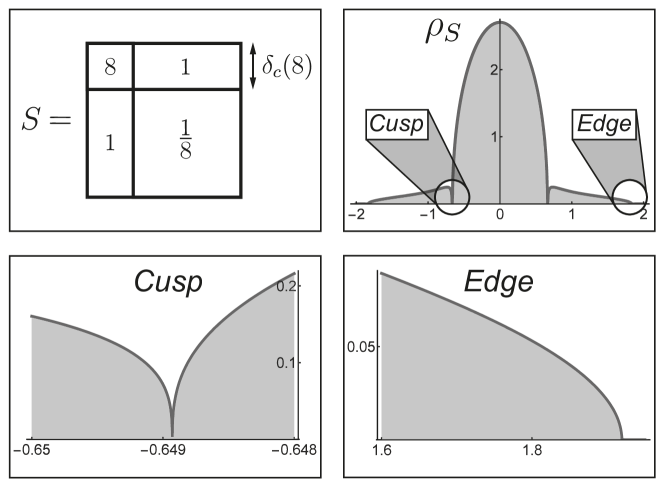
Figure 3.1: $2\times 2$ - block profile whose density has a cusp singularity.

We remark that the solution $m$ of the QVE corresponding to the $2\times 2$-profile (3.2) through $s_{xy}=q(x,y)$ is of the form $m(z)=\mu(z)\mspace{2.0mu}\mathbbm{1}_{I}+\nu(z)\mspace{2.0mu}\mathbbm{1}_{I^{c}}$, for some component functions $\mu,\nu:\mathbb{H}\to\mathbb{H}$. With this ansatz the original QVE reduces to a two dimensional system for the components $(\mu,\nu)$. Already in this simple case solving the QVE for general $\alpha,\beta,\gamma$ already requires solving a quartic polynomial. Nevertheless, Theorem 2.6 shows that a quartic singularity of $\rho_{S}$ never appears.

3.2 Deformed Wigner matrices

Another class of well studied self-adjoint random matrix models are the deformed Wigner matrices of the form

$$H\,=\,A+\lambda V\,,$$

where $A$ is a deterministic diagonal matrix and $V$ is a Wigner matrix, i.e., $V$ has centered i.i.d. entries, up to the symmetry constraints. In the corresponding QVE (2.1), we have $\mathfrak{X}=[0,1]$ with uniform measure, $s_{xy}\equiv\lambda$ and $a_{x}$ the smooth limiting profile of the diagonal entries of $A$. The average generating density $\rho_{S,a}$ equals the asymptotic density of the eigenvalues as the dimension of $H$ approaches infinity [33]. In particular, Theorem 2.6 restricts the possible singularities of the limiting eigenvalue density to at most third order.

The cubic root cusp has been observed in this context in [13] in the case when $V$ is a Gaussian unitarily invariant matrix (GUE) and $A$ has a spectrum symmetric to the origin with a gap around zero. As the coupling constant $\lambda>0$ increases from zero, at a critical value the gap closes in the support of the density and a cubic singularity emerges. The argument in [13], however, did not use the QVE. Since the randomness is generated by a GUE matrix, all local correlation functions can be explicitly computed via the Itzykson-Zuber formula. The cubic root cusp can then be easily recovered from (3.22) in [13]. We remark that in this case the type of singularity also determines the local statistics. Analogously to the Wigner-Dyson statistics in the bulk and the Tracy-Widom statistics at regular edges with a square root behavior, the cubic root singularity gives rise to a determinantal process described by the Pearcey kernel, see e.g. [2, 11, 39].

3.3 Translation invariant correlations

Let $\underline{\xi}=(\xi_{ij}:i,j\in\mathbb{Z})$ be a family of i.i.d. random variables indexed by $\mathbb{Z}^{2}$. Let $\theta_{pq}$, $p,q\in\mathbb{Z}$, denote a shift of $\underline{\xi}$, such that the $(i,j)$-th component of $\theta_{pq}\underline{\xi}$ is $\xi_{i+p,j+q}$. Given a measurable function $\Phi:\mathbb{R}^{\mathbb{Z}^{2}}\to\mathbb{R}$, such that

$$\mathbb{E}\,\Phi(\underline{\xi})=0\,,\qquad\mathbb{E}\,\Phi(\underline{\xi})^{2}<\infty\,,\quad\text{and}\quad\sum_{p,\mspace{1.0mu}q\in\mathbb{Z}}\big{\lvert}\mspace{2.0mu}\mathbb{E}\,\Phi(\theta_{pq}\underline{\xi})\mspace{1.0mu}\Phi(\underline{\xi})\mspace{1.0mu}\big{\rvert}\,<\,\infty\,,$$

we define a sequence of translation invariant random matrices $H=H^{(N)}$ through

$$h_{ij}:=\frac{\Phi(\theta_{ij}\underline{\xi})\mspace{1.0mu}+\mspace{2.0mu}\Phi(\theta_{ji}\underline{\xi})}{\!\sqrt{N\mspace{2.0mu}}}\,.$$

Then their empirical spectral measures converge weakly in probability to a non-random measure with a density $\rho_{S}=\rho_{S\mspace{-1.0mu},0}:\mathbb{R}\to[0,\infty)$. The limiting density $\rho_{S}$ is determined by the solution $m$ of the QVE in the setup $(\mathfrak{X},\pi(\mathrm{d}x))=([0,1],\mathrm{d}x)$, where $S$ has the integral kernel $s:[\mspace{1.0mu}0,1\mspace{1.0mu}]^{2}\to[\mspace{1.0mu}0,\infty)$,

$$s_{xy}\,:=\,4\sum_{p,\mspace{1.0mu}q\in\mathbb{Z}}\mathrm{e}^{-\mspace{1.0mu}\mathrm{i}\mspace{1.0mu}2\mspace{1.0mu}\pi\mspace{1.0mu}(p\mspace{1.0mu}x\mspace{2.0mu}-\mspace{2.0mu}q\mspace{1.0mu}y)}\,\mathbb{E}\,\Phi(\theta_{pq}\underline{\xi})\mspace{1.0mu}\Phi(\underline{\xi})\,,$$

and $a=0$. This convergence has been established in the Gaussian setup in [3, 28, 35]. In [9] it was extended by a comparison argument to the general setting we presented here.

3.4 The color equation

In [7] the authors show that the empirical distributions of the eigenvalues of a class of random matrices with dependent entries converge to a probability measure $\mu$ on $\mathbb{R}$ as the dimension of the matrices becomes large. The measure $\mu$ is determined through the so-called color equations (cf. equation (3.9) on p. 1135):

$$\int_{C}\frac{s(c,c^{\prime})P(\mathrm{d}c^{\prime})}{\lambda-\Psi(c^{\prime},\lambda)}\,=\,\Psi(c,\lambda)\,,\qquad\int_{\mathbb{R}}\frac{\mu(\mathrm{d}\tau)}{\lambda-\tau}=\int_{C}\!\frac{P(\mathrm{d}c)}{\lambda-\Psi(c,\lambda)}\,,$$

where $\lambda\in{\mathbb{C}}$ and the color space is $C=[0,1]\times\mathbb{S}^{1}$, with $\mathbb{S}^{1}$ denoting the unit circle on the complex plane. Identifying $\mathfrak{X}=C$, $x=c$, $y=c^{\prime}$, $\pi(\mathrm{d}x):=P(\mathrm{d}c)$, $z=\lambda$, we see that the color equation is equivalent to the QVE (2.1). Indeed, we have the correspondence

$$s_{xy}=s(c,c^{\prime})\,,\qquad m_{x}(z)=\frac{\!-1\,}{\lambda-\Psi(c,\lambda)}\,,$$

so that from (2.2) we see that $\rho_{S,0}(\mathrm{d}\tau)=\mu(\mathrm{d}\tau)$. Hence our results cover the asymptotic spectral statistics of this large class of random matrices with non-translation invariant correlations as well.

4 Boundedness of the solution

Recall the existence and uniqueness of the solution $m$ to the QVE, as well as the Stieltjes transform representation (cf. Proposition 2.1). In this section we show that $m$ is uniformly bounded, and that the imaginary part of $m$ has mutually comparable components. First we introduce a few notations and conventions that will be used throughout this paper.

Notation (Comparison relation).

For brevity we introduce the concept of comparison relations: If $\varphi=\varphi(u)$ and $\psi=\psi(u)$ are non-negative functions on some set $U$, then the notation $\varphi\lesssim\psi$, or equivalently, $\psi\gtrsim\varphi$, means that there exists a constant $0<C<\infty$, depending only on the data input $s$ and $a$ of the QVE, such that $\varphi(u)\leq C\mspace{1.0mu}\psi(u)$ for all $u\in U$. If $\psi\lesssim\varphi\lesssim\psi$ then we write $\varphi\sim\psi$, and say that $\varphi$ and $\psi$ are comparable. Furthermore, we use $\psi=\varphi+\mathcal{O}(\xi)$ as a shorthand for $\lvert\psi-\phi\rvert\lesssim\xi$, where $\psi$ and $\varphi$ do not have to be non-negative.

Many quantities in the following depend on the spectral parameter $z$, but for brevity we will often drop this dependence from our notation whenever the spectral parameter is considered fixed, e.g., we denote $m=m(z)$.

Proposition 2.1 shows that the component $m_{x}$ of the solution to the QVE is determined by the component $v_{x}(\mathrm{d}\tau)$ of the generating measure with support in $[-\kappa,\kappa]$. The Stieltjes transform representation (2.2) also implies that $v_{x}(\mathrm{d}\tau)$ can be viewed as the weak limit $\lim_{\eta\downarrow 0}\frac{1}{\pi}\operatorname{Im}m_{x}(\tau+\mathrm{i}\mspace{1.0mu}\eta)\mathrm{d}\tau$. We may therefore restrict our analysis of $m$ to spectral parameters $z$ with $\lvert z\rvert\leq 2\kappa$. The following Proposition is the main result of this section.

Proposition 4.1 (Uniform bound).

Let $s$ and $a$ satisfy assumptions (A), (B) and (C). Then the solution $m_{x}(z)$ of the QVE is uniformly bounded and bounded away from zero,

$$\lvert m(z)\rvert\,\sim\,1\,,\qquad\lvert z\rvert\mspace{1.0mu}\leq\mspace{1.0mu}2\kappa\,.$$ (4.1)

Moreover, the components of the imaginary part of $m$ are all comparable in size,

$$\operatorname{Im}m_{x}(z)\,\sim\,\operatorname{Im}m_{y}(z)\,,\qquad x,y\in\mathfrak{X}\,,\;\lvert z\rvert\mspace{1.0mu}\leq\mspace{1.0mu}2\kappa\,.$$ (4.2)

In the following definition we introduce a $z$-dependent operator $F(z)$ that depends on the value $m(z)$ of the solution at $z$. This operator will play a fundamental role in the upcoming analysis and in the proof of Proposition 4.1 in particular.

Definition 4.2 (Operator $F$).

Let $m$ be the solution of the QVE and $z\in\mathbb{H}$. Then we define the operator $F(z)$ on $\mathcal{B}(\mathfrak{X},{\mathbb{C}})$ by

$$(F(z)\mspace{1.0mu}w)_{x}\,:=\,|\mspace{1.0mu}m_{x}(z)|\int s_{xy}\mspace{1.0mu}|\mspace{1.0mu}m_{y}(z)|\mspace{1.0mu}w_{y}\mspace{1.0mu}\pi(\mathrm{d}y)\,,\qquad w\in\mathcal{B}(\mathfrak{X},{\mathbb{C}})\,.$$ (4.3)

We denote by $\lVert\mspace{2.0mu}\cdot\mspace{2.0mu}\rVert_{2}$ the standard norm on $L^{2}(\mathfrak{X})=L^{2}(\mathfrak{X},\pi)$ and by $\lVert T\rVert_{2}$ the induced operator norm of some operator $T$ on $L^{2}(\mathfrak{X})$. We will now see that the diagonal rescaling by $\lvert m\rvert$ in the definition of $F$ implies that the spectral radius of this operator will always be bounded by $1$.

Lemma 4.3 (Spectral radius of $F$).

Let $z\in\mathbb{H}$ and the operator $F(z)$ be as in (4.3). Then the spectral radius $\lVert F(z)\rVert_{2}$ is an eigenvalue of $F(z)$ and there exists at least one corresponding non-negative eigenfunction $f(z)\in\mathcal{B}(\mathfrak{X},\mathbb{R}_{0}^{+})$. Any such eigenfunction satisfies the relation

$$\lVert F(z)\rVert_{2}\,=\,1-\frac{\langle f(z)\mspace{1.0mu}|m(z)|\rangle\operatorname{Im}z}{\langle f(z)|m(z)|^{-1}\operatorname{Im}m(z)\rangle}\,.$$ (4.4)

Proof.

Since the kernel $s$ is bounded and the solution of the QVE satisfies the trivial bound (A.10), the kernel of the integral operator $F$ is bounded as well. This implies that $F$ is compact when it is considered as an operator on $L^{p}(\mathfrak{X})$ with $p\in(1,\infty)$. By the Krein-Rutman theorem the spectral radius $\lVert F\rVert_{2}$ is an eigenvalue of $F$ with a corresponding non-negative eigenfunction $f\in L^{p}(\mathfrak{X})$. From the eigenvalue equation, $Ff=\lVert F\rVert_{2}\mspace{1.0mu}f$, and the boundedness of the kernel of $F$ we read off that $f$ is bounded, i.e., up to modification on a set of measure zero it is an eigenfunction of $F$ as an operator on $\mathcal{B}(\mathfrak{X},{\mathbb{C}})$.

We will now show (4.4). We take the imaginary part on both sides of (2.1) and multiply with $\lvert m\rvert$:

$$|m|^{-1}\operatorname{Im}m\,=\,|m|\mspace{1.0mu}\operatorname{Im}z+F(|m|^{-1}\operatorname{Im}m)\,.$$ (4.5)

Let $f\in\mathcal{B}(\mathfrak{X},\mathbb{R}_{0}^{+})$ be an arbitrary eigenfunction of $F$ corresponding to the eigenvalue $\lVert F\rVert_{2}$. We multiply both sides of (4.5) with $f$ and take the average. Since the kernel of $F$ is symmetric we end up with

$$\langle\mspace{1.0mu}f\mspace{1.0mu}|m|^{-1}\operatorname{Im}m\mspace{1.0mu}\rangle\,=\,\langle\mspace{1.0mu}f\mspace{1.0mu}|m|\mspace{1.0mu}\rangle\mspace{1.0mu}\operatorname{Im}z\,+\mspace{2.0mu}\lVert F\rVert_{2}\mspace{1.0mu}\langle\mspace{1.0mu}f\mspace{1.0mu}|m|^{-1}\operatorname{Im}m\mspace{1.0mu}\rangle\,.$$

This is equivalent to (4.4) and Lemma 4.3 is proven. ∎

Proof of Proposition 4.1.

First we show the uniform upper bound in (4.1). The uniform lower bound will be shown along the way as well. We fix $z\in\mathbb{H}$ with $\lvert z\rvert\leq 2\mspace{1.0mu}\kappa$. We start by establishing boundedness in $L^{2}(\mathfrak{X})$, i.e.,

$$\lVert m\rVert_{2}\,\lesssim\,1\,.$$ (4.6)

Once we have shown (4.6), the uniform bound follows from the following lemma, whose proof is postponed until the end of this section.

Lemma 4.4.

Let $z\in\mathbb{H}$, $\Phi\in\mathbb{R}^{+}$ and $\Gamma_{\!\Phi}:\mathbb{R}^{+}\to\mathbb{R}^{+}$ be the strictly monotonically increasing function defined by

$$\Gamma_{\!\Phi}(\tau):=\inf_{x\mspace{1.0mu}\in\mspace{1.0mu}\mathfrak{X}}\int_{\mathfrak{X}}\!\frac{\,\pi(\mathrm{d}y)}{(\mspace{2.0mu}\tau^{-1}\!+|a_{x}-a_{y}|+\lVert S_{x}-S_{y}\rVert_{2}\mspace{2.0mu}\Phi\mspace{2.0mu})^{\mspace{1.0mu}2}\!}\;.$$ (4.7)

If $\lVert m(z)\rVert_{2}\leq\Phi$ and $\lim_{\tau\to\infty}\Gamma_{\Phi}(\mspace{1.0mu}\tau\mspace{1.0mu})>\Phi^{2}$, then

$$\lVert\mspace{1.0mu}m(z)\rVert\;\leq\;(\mspace{1.0mu}\Gamma_{\Phi})^{-1}\mspace{-1.0mu}(\Phi^{2})\,.$$ (4.8)

In fact, in our setting we have $\Gamma_{\!\Phi}(\mathbb{R}^{+})=\mathbb{R}^{+}$ for all $\Phi$ because of the assumption (C) and therefore Lemma 4.4 always provides a uniform upper bound, given that the solution is bounded in $L^{2}(\mathfrak{X})$.

The proof of (4.6) starts by establishing a bound in $L^{1}(\mathfrak{X})$ first. For this we use that the quadratic form corresponding to $F$, evaluated on the constant function $1$, is bounded by $\lVert F\rVert_{2}$. This spectral norm in turn can be estimated by $\lVert F\rVert_{2}\leq 1$, which is a consequence of (4.4). We therefore find the chain of inequalities,

$$1\,\geq\,\lVert F\rVert_{2}\,\geq\,\langle\mspace{1.0mu}\lvert m\rvert\mspace{2.0mu}S\mspace{1.0mu}\lvert m\rvert\mspace{1.0mu}\rangle\,\geq\,\langle(R\mspace{1.0mu}|m|)^{2}\rangle\,\geq\,\langle\mspace{1.0mu}R\mspace{1.0mu}|m|\mspace{1.0mu}\rangle^{2}\,\geq\,\langle|m|\rangle^{2}\inf_{x\in\mathfrak{X}}(R1)^{2}_{x}.$$

In the third inequality we employed (A), where $R$ has $r_{xy}$ as its kernel, and in the second to last step Jensen’s inequality was used. Thus, $\langle|m|\rangle\lesssim 1$.

This $L^{1}(\mathfrak{X})$-bound is now used to infer that $m$ is bounded away from zero. Indeed, taking absolute value on both sides of the QVE implies

$$\frac{1}{|m|}\,\leq\,|z|+\lVert a\rVert+\langle\mspace{1.0mu}|m|\mspace{1.0mu}\rangle\!\sup_{x,y\mspace{1.0mu}\in\mspace{1.0mu}\mathfrak{X}}s_{xy}\,.$$

In particular, we have $\lvert m\rvert\gtrsim 1$ because $\lvert z\rvert\leq 2\mspace{1.0mu}\kappa$, which proves the uniform lower bound in (4.1).

From this lower bound on the absolute value of the solution, (4.6) follows by using that the $L^{2}(\mathfrak{X})$-norm of $F$ applied to the constant function $1$ is bounded by the spectral radius of $F$,

$$1\,\geq\,\lVert F\rVert_{2}^{2}\,\geq\,\langle(\lvert m\rvert S\lvert m\rvert)^{2}\rangle\,\geq\,\langle\mspace{1.0mu}|m|^{2}\rangle\inf_{x\in\mathfrak{X}}(S|m|)_{x}^{2}\,.$$ (4.9)

The lower bound on $\lvert m\rvert$ indeed yields

$$\inf_{x\mspace{1.0mu}\in\mspace{1.0mu}\mathfrak{X}}(S|m|)_{x}\,\geq\,\inf_{x\mspace{1.0mu}\in\mspace{1.0mu}\mathfrak{X}}(R^{2}|m|)_{x}\,\gtrsim\inf_{x\mspace{1.0mu}\in\mspace{1.0mu}\mathfrak{X}}\Bigl{(}{\int r_{xy}\mspace{1.0mu}\pi(\mathrm{d}y)}\Bigr{)}^{2}>\mspace{2.0mu}0\,,$$

where we used assumption (A) in the first and last inequality. Thus, (4.9) implies (4.6) and hence the uniform bound (4.1).

Now we show (4.2). In fact, we will see that the components of $\operatorname{Im}m$ are comparable to their average, $\operatorname{Im}m_{x}\sim\langle\mspace{1.0mu}\operatorname{Im}m\mspace{1.0mu}\rangle$. We take the imaginary part on both sides of (2.1) and use (4.1) to see that

$$\operatorname{Im}m\,\sim\,\operatorname{Im}z+S\operatorname{Im}m\,.$$ (4.10)

Since $\operatorname{Im}z\geq 0$, we have $\operatorname{Im}m\gtrsim S\operatorname{Im}m$. We iterate this inequality $K$ times and find

$$\operatorname{Im}m\,\gtrsim\,S^{K}\operatorname{Im}m\,\gtrsim\,\langle\mspace{1.0mu}\operatorname{Im}m\mspace{1.0mu}\rangle\,,$$

using assumption (B).

On the other hand, since $\operatorname{Im}m\geq 0$, by averaging on both sides of (4.10) we get $\langle\operatorname{Im}m\rangle\gtrsim\operatorname{Im}z$. Therefore, (4.10) also implies

$$\operatorname{Im}m\,\lesssim\,\langle\mspace{1.0mu}\operatorname{Im}m\mspace{1.0mu}\rangle+S\operatorname{Im}m\,\leq\,\langle\mspace{1.0mu}\operatorname{Im}m\mspace{1.0mu}\rangle+\langle\mspace{1.0mu}\operatorname{Im}m\mspace{1.0mu}\rangle\sup_{x,y\in\mathfrak{X}}s_{xy}\,.$$

This finishes the proof of Proposition 4.1. ∎

Proof of Lemma 4.4.

By adding and subtracting $m_{x}^{-1}$ and using the QVE we obtain

$$\frac{1}{\lvert m_{y}\rvert}\,=\,\bigg{\lvert}\frac{1}{m_{x}\!}+a_{x}-a_{y}+\big{\langle}S_{x}-S_{y},m\big{\rangle}\bigg{\rvert}\,\leq\,\Big{\lvert}\frac{1}{m_{x}\!}\Big{\rvert}+|a_{x}-a_{y}|+\lVert S_{x}-S_{y}\rVert_{2}\lVert m\rVert_{2}\,,$$

for any $y\in\mathfrak{X}$. Applying $t\mapsto t^{-2}$ on both sides, integrating over $y$, and using $\lVert m\rVert_{2}\leq\Phi$, we find

$$\Phi^{2}\geq\!\int_{\mathfrak{X}}\Big{\lvert}\frac{1}{\mspace{2.0mu}m_{y}}\!\Big{\rvert}^{-2}\mspace{-7.0mu}\pi(\mathrm{d}y)\geq\!\int_{\mathfrak{X}}\Big{(}\frac{1}{\lvert\mspace{1.0mu}m_{x}\rvert\!}+|a_{x}-a_{y}|+\lVert S_{x}-S_{y}\rVert_{2}\mspace{2.0mu}\Phi\Big{)}^{\!-2}\mspace{-5.0mu}\pi(\mathrm{d}y)\,\geq\,\Gamma_{\Phi}\big{(}\lvert m_{x}\rvert\big{)}\,,$$

for any $x\in\mathfrak{X}$. This is equivalent to (4.8) since the strictly monotonous function $\Gamma_{\!\Phi}$ is invertible on $\Phi^{2}$ by assumption. ∎

5 Regularity of the solution

From here on we will always assume that $s$ and $a$ satisfy assumptions (A), (B) and (C). In this section we will analyze the regularity of $\operatorname{Im}m(z)$ as a function of $z$. Since the generating density is the limit of $\frac{1}{\pi}\operatorname{Im}m(\tau+\mathrm{i}\eta)$ as $\eta\downarrow 0$, this regularity will be inherited by $v$, provided it is established uniformly in $\eta$. In this spirit, we prove the following proposition.

Proposition 5.1 (Regularity of the generating density).

The generating density $v(\tau)\in\mathcal{B}(\mathfrak{X},\mathbb{R}_{0}^{+})$ exists and is uniformly $1/3$-Hölder continuous in $\tau$,

$$\sup_{\tau_{1}\neq\tau_{2}}\frac{\lVert\mspace{1.0mu}v(\tau_{1})-v(\tau_{2})\rVert}{|\tau_{1}-\tau_{2}|^{1/3}}\,<\,\infty\,.$$

Moreover, $v(\tau)$ is real analytic for $\tau\in\mathbb{R}\backslash\partial\mathfrak{S}$ .

From the comparability (4.2) of the components of $\operatorname{Im}m$ we infer that the components $v_{x}$ of the generating density are comparable as well. In particular, the set $\mathfrak{S}$ as defined in (2.8) does not depend on $x$

Proof of Proposition 5.1.

In order to show that the generating density exists and is $1/3$-Hölder continuous, we will prove that

$$\sup_{z_{1}\neq z_{2}}\frac{\lVert\mspace{1.0mu}\operatorname{Im}m(z_{1})-\operatorname{Im}m(z_{2})\rVert}{|z_{1}-z_{2}|^{1/3}}\,<\,\infty\,,$$ (5.1)

where the supremum is taken over $z_{1},z_{2}\in\mathbb{H}$. In particular, the imaginary part of $m$ can be extended to the real line as a $1/3$-Hölder continuous function on the extended upper half plane $\operatorname{Im}m:\overline{\mathbb{H}}\to\mathcal{B}(\mathfrak{X},\mathbb{R}^{+}_{0})$. Due to the Stieltjes transform representation (2.2), this extension coincides with the generating density on the real line up to a factor of $\pi$, i.e.,

$$v(\tau)\,=\,\pi^{-1}\operatorname{Im}m(\tau)\,,\qquad\tau\in\mathbb{R}\,.$$

If the supremum in (5.1) is taken over $z_{1}$ away from the support of the generating measure, $\lvert z_{1}\rvert\geq 2\mspace{1.0mu}\kappa$, then the finiteness follows from (2.2), the boundedness of $\operatorname{Im}m$ (cf. (4.1)) and $\mathrm{supp}\mspace{2.0mu}v_{x}\subseteq[-\kappa,\kappa\mspace{1.0mu}]$. By symmetry, the same argument is made for $\lvert z_{2}\rvert\geq 2\mspace{1.0mu}\kappa$.

To prove (5.1) with the supremum taken over $z_{1},z_{2}\in\mathbb{H}$ with $\lvert z_{1}\rvert,\lvert z_{2}\rvert\leq 2\kappa$ we differentiate both sides of (2.1) with respect to $z$, multiply by $m^{2}$ and collect the terms involving $\partial_{z}m$ on the left hand side,

$$(1-m(z)^{2}S\mspace{1.0mu})\partial_{z}m(z)\,=\,m(z)^{2}.$$ (5.2)

By the following lemma we can invert the operator $1-m(z)^{2}S$.

Lemma 5.2 (Bulk stability).

Let $z\in\mathbb{H}$ with $\lvert z\rvert\leq 2\kappa$. Then

$$\lVert(\mspace{1.0mu}1-m(z)^{2}S\mspace{1.0mu})^{-1}\rVert\,\lesssim\,\langle\mspace{2.0mu}\operatorname{Im}m(z)\rangle^{-2}.$$ (5.3)

The proof of Lemma 5.2 is provided at the end of this section. We apply the lemma to (5.2) and find $\lVert\partial_{z}m(z)\rVert\lesssim\langle\operatorname{Im}m(z)\rangle^{-2}$ for spectral parameters $\lvert z\rvert\leq 2\mspace{1.0mu}\kappa$. Since $z\mapsto m(z)$ is analytic the Cauchy-Riemann equations yield $2\mspace{1.0mu}\mathrm{i}\partial_{z}\operatorname{Im}m=\partial_{z}m$. We infer that

$$\lvert\partial_{z}\operatorname{Im}m\mspace{1.0mu}\rvert\,\lesssim\,\langle\mspace{1.0mu}\operatorname{Im}m\mspace{1.0mu}\rangle^{-2}\,\lesssim\,(\operatorname{Im}m)^{-2},$$ (5.4)

where we used (4.2) in the last inequality. The differential inequality (5.4) directly implies (5.1).

It remains to show that $v$ is analytic on $\mathfrak{S}$. We fix $\tau_{0}$, with $\langle v(\tau_{0})\rangle>0$, and consider the complex ODE,

$$\begin{split}\partial_{z}w\,&=\,(1-w^{2}S)^{-1}w^{2}\,,\quad w(\tau_{0})\mspace{2.0mu}=\mspace{2.0mu}w_{0}\,,\end{split}$$ (5.5)

for an analytic function $w:\mathbb{D}_{\varepsilon}(\tau_{0})\to\mathcal{B}(\mathfrak{X},{\mathbb{C}})$ on the disc of radius $\varepsilon>0$ around $\tau_{0}$. As initial value we choose $w_{0}:=m(\tau_{0})$. The right hand side of the ODE is an analytic function on a neighborhood of $w_{0}$ in $\mathcal{B}(\mathfrak{X},{\mathbb{C}})$ because $\lVert(1-w_{0}^{2}S)^{-1}\rVert\lesssim\langle v(\tau_{0})\rangle^{-2}$ initially by Lemma 5.2. By standard methods the ODE locally has a unique analytic solution that coincides with the solution $m$ of the QVE on $\mathbb{D}_{\varepsilon}(\tau_{0})\cap\overline{\mathbb{H}}$, provided $\varepsilon$ is sufficiently small. ∎

Proof of Corollary 2.7.

The Stieltjes transform of a Hölder continuous function is again Hölder continuous with the same exponent. This is formally expressed by the following lemma. We refer to, e.g. [32], Sec. 22, for details. ∎

Lemma 5.3.

Let $\mu$ be a uniformly $\alpha$-Hölder continuous function on $\mathbb{R}$ with $\alpha\in(0,1)$. Then its Stietjes-transform,

$$(M\mu)(z)\,=\,\int_{\mathbb{R}}\frac{\mu(\tau)\mathrm{d}\tau}{\tau\mspace{2.0mu}-\mspace{2.0mu}z}\,,\qquad z\in\mathbb{H}\,,$$

is uniformly $\alpha$-Hölder continuous on $\mathbb{H}$. In particular, $M\mu$ can be extended to a uniformly $\alpha$-Hölder continuous function on $\overline{\mathbb{H}}$.

For the proof of Lemma 5.2 we will need more spectral information about the operator $F$ than the simple formula (4.4) for its spectral radius. In particular, we need a uniform spectral gap, whose formal definition is as follows.

Definition 5.4 (Spectral gap).

Let $T:L^{2}(\mathfrak{X})\to L^{2}(\mathfrak{X})$ be a compact self-adjoint operator. The spectral gap $\mathrm{Gap}(T)\geq 0$ is the difference between the two largest eigenvalues of $\lvert T\rvert$ (defined by spectral calculus). If $\lVert T\rVert_{2}$ is a degenerate eigenvalue of $\lvert T\rvert$, then $\mathrm{Gap}(T)=0$.

Lemma 5.5 (Spectral gap of $F\mspace{2.0mu}$).

Let $F(z)$ be as in (4.3) for $\lvert z\rvert\leq 2\kappa$. Then the spectral radius $\lVert F(z)\rVert_{2}\sim 1$ is a non-degenerate eigenvalue with corresponding $\lVert\mspace{2.0mu}\cdot\mspace{2.0mu}\rVert_{2}$-normalized non-negative eigenfunction $f(z)\in\mathcal{B}(\mathfrak{X},\mathbb{R}_{0}^{+})$ satisfying

$$f(z)\,\sim\,1\,.$$ (5.6)

The operator $F(z)$ has a uniform spectral gap

$$\mathrm{Gap}(F(z))\,\sim\,1\,.$$ (5.7)

Proof.

Since $\lvert m\rvert\sim 1$ the operator $F$ has the property (B) in place of $S$. Therefore, $T:=F^{K}/\lVert F^{K}\rVert_{2}$ has a symmetric non-negative kernel $t_{xy}\sim 1$. In particular, $T$ is compact, when viewed as an operator on $L^{2}(\mathfrak{X})$, and by the Krein-Rutman theorem its spectral radius $\lVert T\rVert_{2}=1$ is a non-degenerate eigenvalue with corresponding normalized non-negative eigenfunction $h\in L^{2}(\mathfrak{X})$. By the pointwise boundedness of the kernel of $T$ from both above and below, the eigenvalue equation $h=Th$ implies that $h\sim 1$. The result follows from Lemma 5.6 below, noticing that $f=h$. ∎

Lemma 5.6 (Spectral gap for operators with positive kernel).

Let $T$ be a symmetric compact integral operator on $L^{2}(\mathfrak{X})$ with a non-negative integral kernel $t_{xy}=t_{yx}\geq 0$. Then

$$\mathrm{Gap}(T)\,\geq\,\biggl{(}\!\frac{\,\lVert h\rVert_{2}\!}{\lVert h\rVert}\!\biggr{)}^{2}\!\inf_{x,y\in\mathfrak{X}}t_{xy}\,,$$

where $h$ is an eigenfunction with $Th=\lVert T\rVert_{2}\mspace{1.0mu}h$.

For the convenience of the reader we provide the proof of this standard result in the appendix.

Definition 5.7 (Eigenfunction $f\mspace{2.0mu}$).

Let $z\in\mathbb{H}$ and $F(z)$ be as in (4.3). Then by Lemma 5.5 the eigenvalue $\lVert F(z)\rVert_{2}$ is non-degenerate. We will always denote by $f(z)$ the corresponding $\lVert\mspace{2.0mu}\cdot\mspace{2.0mu}\rVert_{2}$-normalized non-negative eigenfunction.

Proof of Lemma 5.2.

We fix $z\in\mathbb{H}$ with $\lvert z\rvert\leq 2\kappa$ and introduce the notation

$$B\,:=\,m^{-2}\lvert m\rvert^{2}-F\,.$$

First we notice that it suffices to estimate the norm of $B^{-1}$ as an operator on $L^{2}(\mathfrak{X})$ from above, because

$$\lVert\mspace{1.0mu}(\mspace{1.0mu}1-m^{2}S\mspace{1.0mu})^{-1}\rVert\,\lesssim\,\lVert B^{-1}\rVert\,\lesssim\,1+\lVert B^{-1}\rVert_{2}\,.$$ (5.8)

Indeed, the first inequality follows from (4.1) and

$$(\mspace{1.0mu}1-m^{2}S\mspace{1.0mu})w\,=\,\lvert m\rvert^{-1}m^{2}B(\lvert m\rvert^{-1}w)\,,\qquad w\in\mathcal{B}(\mathfrak{X},{\mathbb{C}})\,.$$

For the second inequality in (5.8) we use the following argument.

Suppose $B^{-1}$ exists and is bounded on $L^{2}(\mathfrak{X})$ and let $h\in\mathcal{B}(\mathfrak{X},{\mathbb{C}})$. Then there is some $w\in L^{2}(\mathfrak{X})$ such that $Bw=h$. In particular, by the definition of $B$ we have

$$\lVert w\rVert\,\leq\,\lVert h\rVert+\lVert Fw\rVert\,\leq\,\lVert h\rVert+\lVert m\rVert^{2}\langle\lvert w\rvert\rangle\sup_{x,\mspace{1.0mu}y\mspace{1.0mu}\in\mspace{1.0mu}\mathfrak{X}}s_{xy}\,\lesssim\,\lVert h\rVert+\lVert w\rVert_{2}\,=\,\lVert h\rVert+\lVert B^{-1}h\rVert_{2}\,.$$

Now we use the boundedness of $B^{-1}$ on $L^{2}(\mathfrak{X})$, i.e., $\lVert B^{-1}h\rVert_{2}\,\leq\,\lVert B^{-1}\rVert_{2}\lVert h\rVert$, and (5.8) follows.

It remains to show that $\lVert B^{-1}\rVert_{2}\lesssim\langle\mspace{1.0mu}\operatorname{Im}m\mspace{1.0mu}\rangle^{-2}$. We apply the following lemma, which is proven in the appendix.

Lemma 5.8.

Let $T$ be a compact self-adjoint and $U$ a unitary operator on $L^{2}(\mathfrak{X})$. Suppose that $\mathrm{Gap}(T)>0$ and $\lVert T\rVert_{2}\leq 1$. Then there exists a universal positive constant $C$ such that

$$\lVert(\mspace{1.0mu}U-T\mspace{1.0mu})^{-1}\rVert_{2}\,\leq\,\frac{C}{\mathrm{Gap}(T)\,\lvert\mspace{1.0mu}1-\lVert T\rVert_{2}\langle\mspace{1.0mu}h,Uh\rangle\mspace{1.0mu}\rvert}\,,$$ (5.9)

where $h$ is the normalized eigenvector, corresponding to the non-degenerate eigenvalue $\lVert T\rVert_{2}$ of $T$ and $\langle{\mspace{2.0mu}\cdot\mspace{2.0mu}}\mspace{2.0mu},{\mspace{2.0mu}\cdot\mspace{2.0mu}}\rangle$ denotes the standard scalar product on $L^{2}(\mathfrak{X})$.

With the choice $T:=F$, the unitary multiplication operator $U:=m^{-2}\lvert m\rvert^{2}$ and $\lVert F\rVert_{2}\leq 1$ by (4.4), the lemma implies

$$\lVert B^{-1}\rVert_{2}\,\leq\,\frac{C}{\mathrm{Gap}(F)\mspace{2.0mu}\lvert\mspace{2.0mu}1-\lVert\mspace{1.0mu}F\mspace{1.0mu}\rVert_{2}\langle\mspace{1.0mu}m^{-2}\lvert m\rvert^{2}f^{\mspace{1.0mu}2}\mspace{1.0mu}\rangle\rvert\mspace{2.0mu}}\,\lesssim\,\frac{1}{\operatorname{Re}\bigl{[}\mspace{1.0mu}1-\langle\mspace{1.0mu}\lvert m\rvert^{-2}m^{2}f^{\mspace{1.0mu}2}\mspace{1.0mu}\rangle\mspace{1.0mu}\bigr{]}}\,,$$ (5.10)

where we used $\mathrm{Gap}(F)\sim 1$ from Lemma 5.5 for the second inequality. Since we also have (5.6), (4.1) and (4.2) at our disposal, we can estimate further,

$$\operatorname{Re}\bigl{[}\mspace{2.0mu}1-\langle\mspace{1.0mu}\lvert m\rvert^{-2}m^{2}f^{\mspace{1.0mu}2}\rangle\bigr{]}\,=\,2\mspace{1.0mu}\big{\langle}\mspace{1.0mu}\lvert m\rvert^{-2}(\mspace{1.0mu}\operatorname{Im}m)^{2}f^{\mspace{1.0mu}2}\mspace{1.0mu}\big{\rangle}\,\gtrsim\,\langle\mspace{1.0mu}\operatorname{Im}m\mspace{1.0mu}\rangle^{2}.$$ (5.11)

∎

6 Singularities

In this section we will prove our main result, Theorem 2.6. Its proof relies on a careful analysis of how $m(z)$ changes in $z$ in a neighborhood of a singular point $\tau\in\partial\mathfrak{S}$. This change will be described in leading order by a complex valued scalar function $\Theta$ which satisfies a cubic equation. As a solution to this cubic equation, $\Theta$ can only give rise to square root or cubic root singularities of the generating density at $\tau$.

Definition 6.1 (Extensions to the real line).

Under the assumptions (A), (B) and (C) (which are always assumed here) we extend the solution $m$ of the QVE and all its derived quantities, such as $F$, $f$, etc., to $\overline{\mathbb{H}}$ according to Corollary 2.7. We denote these extensions with the same symbols.

Proposition 6.2 (Cubic equation).

For any given $\tau\in\partial\mathfrak{S}$, the complex valued function

$$\Theta(\omega;\tau)\,:=\,\Big{\langle}f(\tau)\,\frac{m(\tau+\omega)-m(\tau)}{|\mspace{1.0mu}m(\tau)|}\Big{\rangle}\,,\qquad\omega\in[-\kappa,\kappa]\,,$$ (6.1)

describes the change of $m$ around $\tau$ to leading order,

$$m(\tau+\omega)-m(\tau)\;=\;\Theta(\omega;\tau)\mspace{2.0mu}|\mspace{1.0mu}m(\tau)|\mspace{2.0mu}f(\tau)+\mathcal{O}\bigl{(}{\lvert\Theta\rvert^{2}+|\omega|}\bigr{)}.$$ (6.2)

The function $\Theta$ solves the approximate cubic equation,

$$\psi(\tau)\mspace{2.0mu}\Theta(\omega;\tau)^{3}+\sigma(\tau)\mspace{1.0mu}\Theta(\omega;\tau)^{2}+\langle|m(\tau)|f(\tau)\rangle\omega\;=\>e(\omega;\tau)\,,$$ (6.3)

where the error term $e(\omega;\tau)$ satisfies

$$\lvert\mspace{1.0mu}e(\omega;\tau)\rvert\, \lesssim\,|\omega|\lvert\Theta(\omega;\tau)\rvert+|\omega|^{2},$$ (6.4a)

$$\lvert\mspace{1.0mu}\operatorname{Im}e(\omega;\tau)\rvert\, \lesssim\,|\omega|\operatorname{Im}\Theta(\omega;\tau)\,.$$ (6.4b)

The real valued coefficients $\sigma$ and $\psi$ are defined as

$$\sigma(\tau)\,:=\,\big{\langle}\mspace{1.0mu}f(\tau)^{3}\mspace{1.0mu}\mathrm{sign}\mspace{2.0mu}m(\tau)\mspace{1.0mu}\big{\rangle}\,,\qquad\psi(\tau)\,:=\,\mathcal{D}_{\tau}({f(\tau)^{2}\mathrm{sign}\mspace{2.0mu}m(\tau)})\,,$$ (6.5)

where the non-negative quadratic form $\mathcal{D}_{\tau}$ is given by

$$\mathcal{D}_{\tau}(w)\,:=\,\Big{\langle}w\mspace{2.0mu}Q(\tau)\frac{1+F(\tau)}{1-F(\tau)}\mspace{1.0mu}Q(\tau)w\Big{\rangle}\,,\qquad Q(\tau)w\,:=\,w-\langle f(\tau)w\rangle f(\tau)\,,$$ (6.6)

for any $w\in\mathcal{B}(\mathfrak{X},{\mathbb{C}})$. The cubic equation for $\Theta$ is stable in the sense that

$$\psi(\tau)+\sigma(\tau)^{2}\,\sim\,1\,,\qquad\tau\in[-\kappa,\kappa\mspace{2.0mu}]\,.$$ (6.7)

Proof of Proposition 6.2.

We fix $\tau\in\partial\mathfrak{S}$. In particular, $\operatorname{Im}m(\tau)=0$. We will often neglect the dependence of various quantities on $\tau$ in our notation, e.g. $m=m(\tau)$, $Q=Q(\tau)$, $\Theta(\omega)=\Theta(\omega;\tau)$, etc. We start the proof by showing that

$$\lVert F(\tau)\rVert_{2}\,=\,1\,.$$ (6.8)

Since $\tau\mapsto\lVert F(\tau)\rVert_{2}$ is a continuous function, it suffices to show $\lVert F(\widetilde{\tau})\rVert_{2}=1$ for $\widetilde{\tau}\in\mathfrak{S}$. The relation (4.4) extends to $\widetilde{\tau}$ since the denominator on the right hand side is positive when evaluated at that point. In particular, the right hand side of this relation equals $1$ at $\widetilde{\tau}$ since $\operatorname{Im}m(\widetilde{\tau})>0$.

We introduce the scaled difference between the solution of the QVE evaluated at $\tau+\omega$ and at $\tau$,

$$u(\omega)\,:=\,\frac{m(\tau+\omega)-m(\tau)}{\lvert m(\tau)\rvert}\,.$$

Using that $m(\tau)=(\mathrm{sign}\mspace{2.0mu}m(\tau))\lvert m(\tau)\rvert$, the definition of the operator $F$ from (4.3) and the QVE with spectral parameters $z=\tau$ and $z=\tau+\omega$, it is easy to verify that $u$ satisfies the quadratic equation

$$(1-F)u(\omega)\,=\,p\mspace{1.0mu}u(\omega)Fu(\omega)+\omega\lvert m\rvert+\omega p\mspace{1.0mu}\lvert m\rvert u(\omega)\,,\quad p\,:=\,\mathrm{sign}\mspace{2.0mu}m\,.$$ (6.9)

We treat the direction $f$, which constitutes the kernel of $1-F$, separately. Recall that $Q=1-\langle f\,\cdot\,\rangle f$ is the projection onto the orthogonal complement of $f$. We decompose $u$ according to

$$u(\omega)\,=\,\Theta(\omega)\mspace{1.0mu}f+Qu(\omega)\,,\qquad\Theta(\omega)\,=\,\langle f\mspace{1.0mu}u(\omega)\rangle\,.$$ (6.10)

The Hölder continuity of $m$ from Corollary 2.7 leads to the a priori estimate

$$\lvert\Theta(\omega)\rvert+\lVert Qu(\omega)\rVert\,\lesssim\,\lvert\omega\rvert^{1/3}.$$ (6.11)

We will now derive an improved bound for $Qu$. To this end we insert the decomposition (6.10) into (6.9), use the eigenvalue equation $Ff=f$ and project with $Q$ on both sides. A short calculation shows that

$$(1-F)Qu(\omega)\,=\,\Theta(\omega)^{2}\mspace{1.0mu}Q[p\mspace{1.0mu}f^{2}]+e_{1}(\omega)\,,$$ (6.12)

where the error function $e_{1}(\omega)\in\mathcal{B}(\mathfrak{X},{\mathbb{C}})$ satisfies the two bounds

$$\lVert e_{1}(\omega)\rVert\, \lesssim\,\lvert\omega\rvert^{1/3}\lVert Qu(\omega)\rVert+\lvert\omega\rvert\,,$$ (6.13a)

$$\lVert\operatorname{Im}e_{1}(\omega)\rVert\, \lesssim\,\lvert\omega\rvert^{1/3}\lVert\operatorname{Im}Qu(\omega)\rVert+(\mspace{1.0mu}\lVert Qu(\omega)\rVert+\lvert\omega\rvert\mspace{1.0mu})\mspace{2.0mu}\operatorname{Im}\Theta(\omega)\,.$$ (6.13b)

Here we have used (6.11).

Inverting $1-F$ on the orthogonal complement of $f$ in (6.12) and using (6.13a) and (6.13b), respectively, yields the improved bounds

$$\lVert Qu(\omega)\rVert\, \lesssim\,\lvert\Theta(\omega)\rvert^{2}+\lvert\omega\rvert\,,$$ (6.14a)

$$\lVert\operatorname{Im}Qu(\omega)\rVert\, \lesssim\,(\mspace{1.0mu}\lvert\Theta(\omega)\rvert+\lvert\omega\rvert\mspace{1.0mu})\mspace{1.0mu}\operatorname{Im}\Theta(\omega)\,.$$ (6.14b)

For both inequalities, (6.13a) and (6.13b), we have used that $1-F$ is invertible on its image with bounded inverse,

$$\lVert(1-F)^{-1}Q\mspace{1.0mu}\rVert\,\lesssim\;1+\lVert(1-F)^{-1}Q\mspace{1.0mu}\rVert_{2}\,\lesssim\;1\,.$$ (6.15)

The first inequality in (6.15) follows from the same argument as the second inequality in (5.8), while the second inequality is a consequence of the uniform spectral gap estimate (5.7) for $F$. Additionally, for (6.14a) we have used (6.13a) and for (6.14b) we have used (6.13b) in conjunction with (6.14a). In particular, the improved bound (6.14a) on the norm of $Qu$ together with (6.10) shows the validity of (6.2).

Now we will derive the cubic equation (6.3) for $\Theta$. We start by plugging the decomposition (6.10) into (6.9), using $Ff=f$ and projecting on both sides with the linear functional $w\mapsto\langle f\mspace{1.0mu}w\rangle$ onto the $f$-direction,

$$0\,=\,\Theta(\omega)^{2}\langle pf^{3}\rangle+\Theta(\omega)\langle p\mspace{1.0mu}f^{2}(1+F)Qu(\omega)\rangle+\omega\langle f\lvert m\rvert\rangle+e_{2}(\omega)\,.$$ (6.16)

Here, the error term $e_{2}$ satisfies

$$\lvert e_{2}(\omega)\rvert\, \lesssim\,\lVert Qu(\omega)\rVert^{2}+\lvert\omega\rvert\lvert\Theta(\omega)\rvert+\lvert\omega\rvert\lVert Qu(\omega)\rVert\,,$$ (6.17a)

$$\lvert\operatorname{Im}e_{2}(\omega)\rvert\, \lesssim\,\lVert Qu(\omega)\rVert\lVert\operatorname{Im}Qu(\omega)\rVert+\lvert\omega\rvert\lvert\operatorname{Im}\Theta(\omega)\rvert+\lvert\omega\rvert\lVert\operatorname{Im}Qu(\omega)\rVert\,.$$ (6.17b)

Solving for $Qu$ in (6.12) and plugging the resulting expression into (6.16) yields (6.3) with the coefficients $\sigma$ and $\psi$ defined as in (6.5) and the error term $e(\omega)=e_{\tau}(\omega)$ given by

$$e(\omega)\,:=\,-\mspace{1.0mu}e_{2}(\omega)\,-\,\Theta(\omega)\big{\langle}p\mspace{1.0mu}f^{2}(1+F)(1-F)^{-1}e_{1}(\omega)\big{\rangle}\,.$$ (6.18)

It remains to verify the error bounds (6.4) and show the stability of the cubic (6.7). We start with the error bounds by estimating the absolute value,

$$\lvert e(\omega)\rvert\,\lesssim\,\lvert e_{2}(\omega)\rvert+\lvert\Theta(\omega)\rvert\lVert e_{1}(\omega)\rVert\,\lesssim\,\lvert\omega\rvert\lvert\Theta(\omega)\rvert+\lvert\omega\rvert^{2},$$

where in the second inequality we used (6.17a), (6.13a), (6.14a) and (6.11) in that order.

Now we estimate the imaginary part of $e(\omega)$. From its definition (6.18) we read off the first inequality in

$$\lvert\mspace{1.0mu}\operatorname{Im}e(\omega)\rvert\,\lesssim\,\lvert\mspace{1.0mu}\operatorname{Im}e_{2}(\omega)\rvert+\lVert e_{1}(\omega)\rVert\mspace{2.0mu}\operatorname{Im}\Theta(\omega)+\lvert\Theta(\omega)\rvert\lVert\mspace{1.0mu}\operatorname{Im}e_{1}(\omega)\rVert\,\lesssim\,\lvert\omega\rvert\operatorname{Im}\Theta(\omega)\,.$$

For the second estimate we used (6.17b), (6.13a), (6.13b), (6.14a), (6.14b) and (6.11) one after the other.

Finally, we show (6.7). Only the lower bound requires a proof. First we observe that, by Definition 5.4 of the spectral gap, and by $\lVert F\rVert_{2}\leq 1$, the quadratic form $\mathcal{D}$, defined in (6.6), satisfies the lower bound

$$\mathcal{D}(w)\,\geq\,\frac{\mathrm{Gap}(F)}{2}\,\lVert Qw\rVert_{2}^{2}\,,\qquad w\in\mathcal{B}(\mathfrak{X},{\mathbb{C}})\,.$$

With the choice $w:=pf^{2}$ we conclude that

$$\psi+\sigma^{2}\,=\,\mathcal{D}(w)+\langle f\mspace{1.0mu}w\rangle^{2}\,\geq\,\frac{\mathrm{Gap}(F)}{2}\lVert Qw\rVert_{2}^{2}+\lVert(1-Q)w\rVert_{2}^{2}\,\gtrsim\,\lVert w\rVert^{2}_{2}\,\geq\,1\,,$$

where we used (5.7) in the second to last estimate and the normalization of $f$ together with Jensen’s inequality in the last step. This finishes the proof of Proposition 6.2. ∎

We are now ready to prove Theorem 2.6. Proposition 6.2 reveals that the difference $m(\tau+\omega)-m(\tau)$ at a singular point $\tau\in\partial\mathfrak{S}$ is mainly determined by $\Theta(\omega)$. The cubic equation (6.3) for this quantity is stable in the sense that the second and third order coefficient cannot vanish at the same time (cf. (6.7)). We therefore expect $\Theta$ to only allow for algebraic singularities of order not higher than three. This expectation is supported by the $1/3$-Hölder regularity, established in Corollary 2.7. In fact, since all solutions of (6.7) can be found to leading order explicitly, most of the proof of Theorem 2.6 is concerned with selecting the correct solution branch of (6.3).

Proof of Theorem 2.6.

Taking into account the statements of Propositions 4.1 and 5.1, it remains to show the behavior (2.9) and (2.10) as the value of the generating density approaches zero and that $\mathfrak{S}$ consists of only finitely many intervals. The latter will be shown at the very end of the proof.

Let us fix $\tau\in\partial\mathfrak{S}$. We start by considering the case where $\sigma(\tau)=0$, with $\sigma$ given by (6.5). Within the proof we will see that this characterizes the cusp singularities.

Cusp: Let $\sigma(\tau)=0$. We apply Proposition 6.2. The cubic equation (6.3) takes the simplified form

$$\psi\mspace{2.0mu}\Theta(\omega)^{3}+\langle|m|f\mspace{1.0mu}\rangle\mspace{1.0mu}\omega\,=\,e(\omega)\,,$$ (6.19)

where $e(\omega)$ satisfies (6.4) and $\psi\sim 1$ according to (6.7). Since $\lvert m\rvert,f\sim 1$ and $m(z)$ is uniformly $1/3$-Hölder continuous in $z$ (cf. (2.11)), the function $\Theta(\omega)$ inherits the regularity of $m$ by its definition in (6.1). In particular, $\lvert\Theta(\omega)\rvert\lesssim\lvert\omega\rvert^{1/3}$ and (6.4a) implies

$$e(\omega)\,=\,\mathcal{O}(\lvert\omega\rvert^{4/3})\,.$$

A simple perturbative calculation of the solution of (6.19) shows that $\Theta$ has the form

$$\Theta(\omega)\;=\;\widehat{\Theta}_{p}(\omega)\mathbbm{1}(\omega<0)\mspace{2.0mu}+\,\widehat{\Theta}_{q}(\omega)\mathbbm{1}(\omega\geq 0)\,+\,\mathcal{O}(\lvert\omega\rvert^{2/3})\,,$$ (6.20)

where $\widehat{\Theta}_{\#}$ is the solution of (6.19) if the error term on the right hand side is set equal to zero, i.e.,

$$\widehat{\Theta}_{\#}(\omega)\,:=\,-\mspace{2.0mu}\zeta_{\#}\;(\mathrm{sign}\,\omega)\biggl{(}{\!\frac{\langle|m|f\rangle}{\psi}\,\lvert\omega\rvert}\biggr{)}^{\!1/3},\qquad\#=0,\pm\,.$$ (6.21)

Here, $\zeta_{0}=1$ and $\zeta_{\pm}=(-1\pm\mathrm{i}\sqrt{3})/2$ are the cubic roots of unity. We will now show that $p=+$ and $q=-$ for the indices in (6.20).

First we rule out the choice $p=-$, as well as the choice $q=+$. Indeed, in both cases the imaginary part of the corresponding $\Theta(\omega)$ would have negative values for $\omega<0$ and $\omega>0$, respectively. This is contradictory to the definition of $\Theta$ in (6.1) and to the fact that $\operatorname{Im}m(\tau)=0$ and $\operatorname{Im}m(\tau+\omega)\geq 0$.

Suppose now that $p=0$ or $q=0$. Then from the explicit form (6.21) of the leading order term to $\Theta$ we read off that there is a positive constant $c_{1}\sim 1$ such that

$$\lvert\mspace{1.0mu}\operatorname{Re}\Theta(\omega)\rvert\,\sim\,\lvert\omega\rvert^{1/3},\qquad\operatorname{Im}\Theta(\omega)\,\lesssim\,\lvert\omega\rvert^{2/3},$$ (6.22)

on the corresponding side of $\omega=0$, i.e., for $\omega\in[-c_{1},0\mspace{1.0mu}]$ or $\omega\in[\mspace{1.0mu}0,c_{1}]$, respectively. Taking the imaginary part on both sides of the cubic (6.19) this implies that

$$\lvert\omega\rvert^{2/3}\operatorname{Im}\Theta(\omega)\,\lesssim\,(\operatorname{Im}\Theta(\omega))^{3}+\lvert\omega\rvert\operatorname{Im}\Theta(\omega)\,\lesssim\,\lvert\omega\rvert\operatorname{Im}\Theta(\omega)\,,$$ (6.23)

where we used the estimate (6.4b) on the error term $e(\omega)$ to get the first estimate. For the second inequality we have used (6.22) to bound $\operatorname{Im}\Theta$. From (6.23) we conclude that there is a positive constant $c_{2}\sim 1$ such that

$$\operatorname{Im}\Theta(\omega)\,=\,0\qquad\text{ for }\quad\begin{cases}\omega\in[-c_{2},0\mspace{1.0mu}]&\text{ if }\;p\mspace{2.0mu}=\mspace{2.0mu}0\,,\\ \omega\in[\mspace{1.0mu}0,c_{2}]&\text{ if }\;q\mspace{2.0mu}=\mspace{2.0mu}0\,.\end{cases}$$ (6.24)

In particular, the generating density vanishes in either case on the corresponding interval by the definition of $\Theta$ and $\operatorname{Im}m(\tau)=0$. On the other hand, from the formula (6.21) for the leading order term $\widehat{\Theta}_{0}$ to $\Theta$ in (6.20) we see that the real valued $\Theta$ is decreasing somewhere inside these gaps in the support of the generating density, because

$$\Theta(\omega)\,=\,\widehat{\Theta}_{0}(\omega)\mspace{1.0mu}(\mspace{1.0mu}1+\mathcal{O}(\lvert\omega\rvert^{1/3}))\,=\,-\mspace{2.0mu}C_{1}\mspace{2.0mu}\mathrm{sign}(\omega)\mspace{1.0mu}\lvert\omega\rvert^{1/3}(\mspace{1.0mu}1+\mathcal{O}(\lvert\omega\rvert^{1/3}))\,,$$

with a positive constant $C_{1}>0$. Using (6.2) to write

$$m(\tau+\omega)-m(\tau)\,=\,|\mspace{1.0mu}m(\tau)|\mspace{2.0mu}f(\tau)\mspace{2.0mu}\Theta(\omega;\tau)\mspace{1.0mu}(\mspace{1.0mu}1+\mathcal{O}(\lvert\omega\rvert^{1/3}))\,,$$

we see that correspondingly $m$ would have to decrease as well. This contradicts the Stieltjes transform representation (2.2) of $m$, because the Stieltjes transform of a positive measure is monotonically increasing away from the support of that measure, when evaluated on the real line. Having ruled out the choices $p=-$ and $q=+$ earlier, we conclude that $p=+$ and $q=-$.

By (6.2) the function $\Theta$ describes the leading order of the difference between $m(\tau)$ to $m(\tau+\omega)$. Considering only the imaginary part and using the identity $\operatorname{Im}m(\tau+\omega)=\pi\mspace{2.0mu}v(\tau+\omega)$ we find

$$v(\tau+\omega)\,=\,|m(\tau)|\mspace{2.0mu}f(\tau)\operatorname{Im}\Theta(\omega;\tau)+\mathcal{O}(\lvert\omega\rvert^{2/3})\,.$$ (6.25)

From this (2.9) follows if we define $c\in\mathcal{B}(\mathfrak{X},\mathbb{R}^{+})$ by

$$c_{x}\,:=\,\frac{\!\sqrt{3\mspace{2.0mu}}}{2\pi}\biggl{(}{\frac{\langle\mspace{1.0mu}|\mspace{1.0mu}m(\tau)|\mspace{2.0mu}f(\tau)\mspace{1.0mu}\rangle}{\psi(\tau)}}\biggr{)}^{1/3}\!|\mspace{1.0mu}m_{x}(\tau)|\mspace{2.0mu}f_{x}(\tau)\,.$$

The behavior (6.25) of the generating density around $\tau$ with $\sigma(\tau)=0$ shows that such a $\tau\in\partial\mathfrak{S}$ belongs to the intersection of the closure of two connected component of $\mathfrak{S}$, i.e., $\tau$ is a cusp in the sense of the statement of Theorem 2.6. It also verifies (2.9) at such an expansion point $\tau$.

Edge: Let $\sigma=\sigma(\tau)\neq 0$. We will show that $\tau$ is not a cusp. More precisely, we will show that with $\theta:=\mathrm{sign}\mspace{2.0mu}\sigma$ the generating density satisfies

$$v(\tau+\theta\omega)\,=\,\begin{cases}c\mspace{1.0mu}\lvert\omega\rvert^{1/2}+\mathcal{O}(\lvert\omega/\sigma^{2}\rvert)&\text{ if }\;\theta\omega\in[\mspace{1.0mu}0,c_{3}\lvert\sigma\rvert^{3}]\,,\\ 0&\text{ if }\;\theta\omega\in[-c_{3}\lvert\sigma\rvert^{3},\mspace{1.0mu}0\mspace{1.0mu}]\,,\end{cases}$$ (6.26)

for some $c\in\mathcal{B}(\mathfrak{X},\mathbb{R}^{+})$ and some constant $c_{3}\sim 1$.

We will again make use of Proposition 6.2. We write the corresponding cubic equation (6.3) in the form

$$\sigma\mspace{1.0mu}\Theta(\omega)^{2}+\langle|m|f\rangle\mspace{1.0mu}\omega\,=\,e_{3}(\omega)\,,$$ (6.27)

where the cubic term in $\Theta$ is considered part of the error,

$$e_{3}(\omega)\,:=\,e(\omega)-\psi\mspace{1.0mu}\Theta(\omega)^{3}.$$

With the bound (6.4) on $\lvert e(\omega)\rvert$ and the a priori estimate $\lvert\Theta(\omega)\rvert\lesssim\lvert\omega\rvert^{1/3}$ (cf. (6.11)) we see from (6.27) that $\Theta$ satisfies for some positive constant $c_{4}\sim 1$ the bound

$$\lvert\Theta(\omega)\rvert\,\lesssim\,\lvert\omega/\sigma\rvert^{1/2},\qquad\omega\in[-c_{4}\lvert\sigma\rvert^{3},c_{4}\lvert\sigma\rvert^{3}]\,.$$

In particular, $\lvert e_{3}(\omega)\rvert\lesssim\lvert\omega/\sigma\rvert^{3/2}$. We conclude that as a continuous solution of (6.27) the function $\Theta$ has the form

$$\Theta(\omega)\,=\,\widehat{\Theta}_{p}(\omega)\mathbbm{1}(\theta\omega<0)+\widehat{\Theta}_{q}(\omega)\mathbbm{1}(\theta\omega\geq 0)+\mathcal{O}(\lvert\omega/\sigma^{2}\rvert)\,,$$ (6.28)

with $p,q\in\{+,-\}$. Here, $\widehat{\Theta}_{\#}$ denotes the solution of (6.27) with vanishing error term,

$$\widehat{\Theta}_{\pm}(\omega)\,:=\,\biggl{(}{\!\frac{\langle\mspace{1.0mu}|m|\mspace{1.0mu}f\mspace{1.0mu}\rangle}{\lvert\sigma\rvert}\!}\biggr{)}^{\!1/2}\mspace{-7.0mu}\times\begin{cases}\pm\mathrm{i}\lvert\omega\rvert^{1/2},&\;\theta\omega\geq 0\,,\\ \pm\lvert\omega\rvert^{1/2},&\;\theta\omega<0\,.\end{cases}$$ (6.29)

First we notice that for the indices in (6.28) the choice $q=-$ is impossible, because it violates $\operatorname{Im}\Theta\geq 0$, as can be seen from

$$\operatorname{Im}\Theta(\omega)\,=\,\operatorname{Im}\widehat{\Theta}_{b}(\omega)\bigl{(}{\mspace{1.0mu}1+\mathcal{O}\bigl{(}{\lvert\omega/\sigma^{3}\rvert^{1/2}}\bigr{)}}\bigr{)}\,,$$

for $\theta\omega\geq 0$. Thus, the behavior (6.26) of the generating density is proven for $\theta\omega\geq 0$ by taking the imaginary part of (6.2) and defining

$$c_{x}\,:=\,\frac{1}{\pi}\biggl{(}{\frac{\langle|m(\tau)|f(\tau)\rangle}{\lvert\sigma(\tau)\rvert}}\biggr{)}^{1/2}\!|\mspace{1.0mu}m_{x}(\tau)|\mspace{2.0mu}f_{x}(\tau)\,.$$

Now we show that there is a gap in the support of the generating density for $\theta\omega\in[-c_{3}\lvert\sigma\rvert^{3},0]$, i.e., we show that $\operatorname{Im}\Theta(\omega)$ vanishes for these values of $\omega$. The explicit form of $\widehat{\Theta}_{\pm}$ in (6.29) and (6.28) reveal that

$$\lvert\mspace{1.0mu}\operatorname{Re}{\Theta(\omega)}\rvert\,\sim\,\lvert\omega/\sigma\rvert^{1/2},\qquad\operatorname{Im}\Theta(\omega)\,\lesssim\,\lvert\omega/\sigma^{2}\rvert\,,$$ (6.30)

as long as $\theta\omega\in[-c_{5}\lvert\sigma\rvert^{3},0]$ for some constant $c_{5}\sim 1$. Knowing the size of $\operatorname{Re}\Theta$ from (6.30) we take the imaginary part of the quadratic equation (6.27) and find

$$\lvert\sigma\omega\rvert^{1/2}\operatorname{Im}\Theta\,\lesssim\,\lvert\mspace{1.0mu}\operatorname{Im}(\Theta^{3})\rvert+\lvert\omega\rvert\operatorname{Im}\Theta\,\lesssim\,\lvert\omega/\sigma\rvert\operatorname{Im}\Theta\,.$$ (6.31)

Here, (6.4) was used in the first, and (6.30) as well as $\lvert\omega\rvert\lesssim\lvert\sigma\rvert^{3}$ in the second inequality. From (6.31) we conclude that $\operatorname{Im}\Theta(\omega)=0$ for $\theta\omega\in[-c_{3}\lvert\sigma\rvert^{3},0]$ for some positive constant $c_{3}\sim 1$.

This finishes the proof of (6.26). In particular, we see that $\tau$ is not a cusp in the sense of the statement of Theorem 2.6. We also conclude that (2.10) holds true at such an expansion point $\tau$, apart from the fact that the function $\lvert\omega/\sigma\rvert$ inside the $\mathcal{O}$-notation in (6.26) still depends on the uncontrolled quantity $\lvert\sigma\rvert$. This will be remedied by the fact that there can only be finitely many such points, because $\partial\mathfrak{S}$ is a finite set, as we will show below. We may then estimate the quantity $\lvert\sigma\rvert$ inside the error terms by the constant $\min\{\lvert\sigma(\tau)\rvert:\tau\in\partial\mathfrak{S},\,\sigma(\tau)\neq 0\}>0$.

In order to show that $\partial\mathfrak{S}$ is finite we derive a contradiction by assuming the contrary. Since $\mathfrak{S}$ is bounded (Proposition 2.1) it follows that the closed infinite set $\partial\mathfrak{S}$ contains an accumulation point $\tau_{\ast}\in\partial\mathfrak{S}$. If $\sigma(\tau_{\ast})=0$, then $v(\tau_{\ast}+\omega)>0$ for every $\lvert\omega\rvert\in(0,\varepsilon)$, and some $\varepsilon>0$, by the already proven expansion (2.9) for such points $\tau_{\ast}$. This contradicts $\tau_{\ast}\in\partial\mathfrak{S}$, because the generating density vanishes at every point of $\partial\mathfrak{S}$. Thus, we have $\sigma(\tau_{\ast})\neq 0$. Using the expansion (6.26) at $\tau=\tau_{\ast}$ we see that $\tau_{\ast}$ is isolated from other elements of $\partial\mathfrak{S}$ by a distance $c_{3}\mspace{1.0mu}\lvert\sigma(\tau_{\ast})\rvert^{3}>0$. This contradicts $\tau_{\ast}$ being an accumulation point of $\partial\mathfrak{S}$ as well. Hence, we arrive at the conclusion that $\partial\mathfrak{S}$ is finite. This finishes the proof of our main result, Theorem 2.6. ∎

Proof of Theorem 2.8.

Suppose $\tau_{0}\in\partial\mathfrak{S}$. In particular, $m(\tau_{0})$ is real. We will first show that under the assumption (2.12) on $S$ and $a$ the solution $m$ has a definite sign at $\tau_{0}$. More precisely, we show that there exists $\theta=\theta(\tau_{0})\in\{\pm 1\}$ such that

$$\mathrm{sign}\,m_{x}(\tau_{0})=\theta\,,\qquad\forall\mspace{1.0mu}x\in\mathfrak{X}\,.$$ (6.32)

For the proof, we use the QVE to obtain

$$m_{x}(\tau)-m_{y}(\tau)\,=\,m_{x}(\tau)\mspace{2.0mu}m_{y}(\tau)\mspace{2.0mu}\bigl{(}{\,a_{x}-a_{y}+\langle\mspace{1.0mu}m\,(S_{x}-S_{y})\rangle\,}\bigr{)}\,,$$ (6.33)

for every $x,y\in\mathfrak{X}$ and $\tau\in\mathbb{R}$. Suppose now that (6.32) is not true, so that the set

$$\mathfrak{A}\,:=\,\bigl{\{}x\in\mathfrak{X}:\;m_{x}(\tau_{0})>0\bigr{\}}\,.$$

is not trivial. Choosing $x\in\mathfrak{A}$, $y\notin\mathfrak{A}$ and $\tau=\tau_{0}$ in (6.33) yields

$$1\,\lesssim\,m_{x}(\tau_{0})-m_{y}(\tau_{0})\,\lesssim\,\lvert a_{x}-a_{y}\rvert+\langle\mspace{1.0mu}\lvert S_{x}-S_{y}\rvert\mspace{1.0mu}\rangle\,,$$

where in the first estimate we used the lower bound $\lvert m\rvert\gtrsim 1$ and in the second estimate the upper bound $\lvert m\rvert\lesssim 1$ from (4.1). Taking the infimum over $x\in\mathfrak{A}$ and $y\not\in\mathfrak{A}$ contradicts the assumption (2.12). Hence, we conclude that either $\mathfrak{A}=\emptyset$ or $\mathfrak{A}=\mathfrak{X}$, which is equivalent to (6.32).

We will now show that $\tau_{0}$ is either the very right or the very left edge of $\mathfrak{S}$, i.e., we prove that either the generating density vanishes on $[\tau_{0},\infty)$ or on $(-\infty,\tau_{0}]$. Thus, $\partial\mathfrak{S}$ consists of only two points and $\mathfrak{S}$ is a single interval.

First we rule out the possibility that $\tau_{0}$ is a cusp. Using (6.32) in the definition (6.5) of $\sigma$ we conclude that $\sigma(\tau_{0})\neq 0$ and $\mathrm{sign}\,\sigma(\tau_{0})=\theta$. From (6.26), in the proof of Theorem 2.6, we see that $\tau_{0}$ is not a cusp, and that there is a non-trivial connected component $I$ of $\mathbb{R}\backslash\mathfrak{S}$ containing $\tau_{0}$. The expansion (6.26) also implies that $I$ continues in the direction $-\theta$ from $\tau_{0}$. From here on we restrict the discussion to $\theta=-1$. The case $\theta=+1$ is treated analogously.

We will now finish the proof by showing that $I=[\tau_{0},\infty)$. By the continuity of $m(\tau)$ in $\tau$ and the lower bound $\lvert m\rvert\gtrsim 1$ from (4.1) the sign of $m$ stays constant on the interval $I\cap[\tau_{0},2\kappa]$. For $\tau>2\kappa$ we have $m(\tau)<0$ by (2.2). Therefore, (6.32) extends to

$$\mathrm{sign}\,m(\tau)=-1\,,\qquad\forall\,\tau\in I\,.$$ (6.34)

All the components $\tau\mapsto m_{x}(\tau)$ are strictly increasing functions on $I$. This is a consequence of $m_{x}$ being the Stieltjes transform (cf. (2.2)) of the non-negative density $v_{x}$ which vanishes on $I$. Combining this with (6.34) we deduce that $\tau\mapsto\lvert\mspace{1.0mu}m_{x}(\tau)\rvert$ is strictly decreasing for all $x\in\mathfrak{X}$. Decreasing $\lvert m\rvert$ also decreases the spectral radius of the operator $F$, defined in (4.3). In particular, $\lVert F(\tau)\rVert_{2}$ decreases strictly as $\tau\in I$ is moved away from $\tau_{0}$. In particular,

$$\lVert F(\tau_{0})\rVert_{2}\,>\,\lVert F(\tau)\rVert_{2}\,,\qquad\forall\,\tau\in I\backslash\{\tau_{0}\}\,.$$ (6.35)

Since from (6.8) we know that $\lVert F(\tau)\rVert_{2}=1$ for any $\tau\in\partial\mathfrak{S}$, (6.35) implies that $I$ does not contain an element of $\partial\mathfrak{S}$ other than $\tau_{0}$. This completes the proof of Theorem 2.8. ∎

Appendix A Existence and uniqueness

Existence and uniqueness of (2.1) is established by interpreting the QVE as a fixed point equation for a holomorphic map in an appropriately chosen function space. The choice of the correct metric on this space follows naturally from the general theory by Earle and Hamilton [17]. The same line of reasoning has appeared before in a context close to ours in [21, 26, 27].

Proof of Proposition 2.1.

We will set up the fixed point problem on the set of functions defined on the domain

$$\mathbb{H}_{\eta}\,:=\,\bigl{\{}z\in\mathbb{H}\,:\;\operatorname{Im}z\mspace{2.0mu}\geq\mspace{2.0mu}\eta\,,\;\lvert z\rvert\mspace{2.0mu}\leq\mspace{2.0mu}\eta^{-1}\bigr{\}}\,.$$

More precisely, for any $\eta\in(0,\min\{1,\lVert a\rVert^{-1}\})$ we consider the function space

$$\!\mathfrak{B}_{\mspace{-1.0mu}\eta}:=\biggl{\{}\mathfrak{u}:\mathbb{H}_{\mspace{1.0mu}\eta}\to\mathcal{B}(\mathfrak{X},\mathbb{H}):\inf_{z\in\mathbb{H}_{\eta}}\!\operatorname{Im}\mathfrak{u}(z)\geq\frac{\eta^{3}}{(2+\lVert S\rVert)^{2}},\,\sup_{z\in\mathbb{H}_{\mspace{1.0mu}\eta}}\lVert\mathfrak{u}(z)\rVert\leq\frac{1}{\eta}\biggr{\}},$$ (A.1)

equipped with the metric

$$d_{\mathfrak{B}}(\mathfrak{u},\mathfrak{w})\,:=\,\sup_{z\in\mathbb{H}_{\mspace{1.0mu}\eta}}\sup_{x\in\mathfrak{X}}d_{\mathbb{H}}(\mathfrak{u}_{x}(z),\mathfrak{w}_{x}(z))\,,\qquad\mathfrak{u},\mathfrak{w}\in\mathfrak{B}_{\mspace{-1.0mu}\eta}\,,$$

where $d_{\mathbb{H}}$ denotes the standard hyperbolic metric on $\mathbb{H}$. The metric function space $(\mathfrak{B}_{\mspace{-1.0mu}\eta},d_{\mathfrak{B}})$ is complete. In this setting the QVE takes the form

$$\mathfrak{u}\,=\,\Phi(\mathfrak{u})\,,$$ (A.2)

where the function $\Phi$ is defined as

$$\Phi(\mathfrak{u})(z)\,:=\,-\mspace{2.0mu}\frac{1}{z+a+S\mspace{1.0mu}\mathfrak{u}(z)}\,,\qquad\mathfrak{u}\in\mathfrak{B}_{\mspace{-2.0mu}\eta}\,,\;z\in\mathbb{H}_{\mspace{1.0mu}\eta}\,.$$ (A.3)

We will now verify that $\Phi$ is well defined as a map from $\mathfrak{B}_{\mspace{-1.0mu}\eta}$ to itself. In fact, $\Phi$, defined as in (A.3), maps all functions $\mathfrak{u}:\mathbb{H}\to\mathcal{B}(\mathfrak{X},\mathbb{H})$ to functions with the upper bound

$$\lvert\mspace{1.0mu}\Phi(\mathfrak{u})(z)\rvert\,=\,\frac{1}{\lvert z+a+S\mspace{1.0mu}\mathfrak{u}(z)\rvert}\,\leq\,\frac{1}{\operatorname{Im}(z+a+S\mspace{1.0mu}\mathfrak{u}(z))}\,\leq\,\frac{1}{\operatorname{Im}\mspace{1.0mu}z}\,,$$ (A.4)

where we used that $S$ has a non-negative kernel and therefore $\operatorname{Im}S\mspace{1.0mu}\mathfrak{u}(z)\geq 0$. Taking the supremum over all $z\in\mathbb{H}_{\mspace{1.0mu}\eta}$ in (A.4) reveals that $\sup_{z\in\mathbb{H}_{\eta}}\lVert\Phi(\mathfrak{u})(z)\rVert\leq\eta^{-1}$, which is the upper bound in the definition (A.1) of $\mathfrak{B}_{\mspace{-1.0mu}\eta}$.

On the other hand, for every function $\mathfrak{u}:\mathbb{H}_{\mspace{1.0mu}\eta}\to\mathcal{B}(\mathfrak{X},\mathbb{H})$ that satisfies the upper bound $\sup_{z\in\mathbb{H}_{\mspace{1.0mu}\eta}}\lVert\mathfrak{u}(z)\rVert\mspace{2.0mu}\leq\mspace{2.0mu}\eta^{-1}$, we find a lower bound on the imaginary part of $\Phi(\mathfrak{u})$,

$$\operatorname{Im}\Phi(\mathfrak{u})(z)=\frac{\operatorname{Im}(z+a+S\mspace{1.0mu}\mathfrak{u}(z))}{\lvert z+a+S\mspace{1.0mu}\mathfrak{u}(z)\rvert^{2}}\geq\frac{\operatorname{Im}z}{(\lvert z\rvert+\lVert a\rVert+\lVert S\rVert\eta^{-1})^{2}}\geq\frac{\eta^{3}}{(2+\lVert S\rVert)^{2}}\,,$$ (A.5)

for every $z\in\mathbb{H}_{\mspace{1.0mu}\eta}$. Thus, $\Phi:\mathfrak{B}_{\mspace{-1.0mu}\eta}\to\mathfrak{B}_{\mspace{-1.0mu}\eta}$ is well defined.

The two computations in (A.4) and (A.5) also show that the restriction $m|_{\mathbb{H}_{\eta}}$ of any solution to the QVE automatically belongs to $\mathfrak{B}_{\mspace{-1.0mu}\eta}$. In particular, showing existence and uniqueness of the solution $\mathfrak{u}$ to the fixed point equation (A.2) on $\mathfrak{B}_{\mspace{-1.0mu}\eta}$ for every positive $\eta<\min\{1,\lVert a\rVert^{-1}\}$ is equivalent to showing existence and uniqueness of the solution $m:\mathbb{H}\to\mathcal{B}(\mathfrak{X},\mathbb{H})$ to the QVE.

We will now establish a certain contraction property of the map $\Phi$. This property is expressed in terms of the function

$$D(\zeta,\omega)\,:=\,\frac{\lvert\mspace{1.0mu}\zeta-\omega\rvert^{2}}{(\operatorname{Im}\,\zeta)(\operatorname{Im}\,\omega)}\,,\qquad\zeta,\,\omega\in\mathbb{H}\,,$$ (A.6)

which is related to the standard hyperbolic metric $d_{\mathbb{H}}$ by

$$D(\zeta,\omega)\,=\,2\mspace{2.0mu}(\cosh d_{\mathbb{H}}(\zeta,\omega)-1)\,.$$ (A.7)

Lemma A.1 (Contraction property of $\Phi$).

For any $\mathfrak{u},\mathfrak{w}\in\mathfrak{B}_{\mspace{-1.0mu}\eta}$ the map $\Phi:\mathfrak{B}_{\mspace{-1.0mu}\eta}\to\mathfrak{B}_{\mspace{-1.0mu}\eta}$ has the contraction property

$$\sup_{z\in\mathbb{H}_{\eta}}\sup_{x\in\mathfrak{X}}D(\Phi(\mathfrak{u})_{x}(z),\Phi(\mathfrak{w})_{x}(z))\,\leq\,\bigg{(}1+\frac{\,\eta^{2}}{\lVert S\rVert}\bigg{)}^{-2}\mspace{-5.0mu}\sup_{z\in\mathbb{H}_{\eta}}\sup_{x\in\mathfrak{X}}D(\mathfrak{u}_{x}(z),\mathfrak{w}_{x}(z))\,.$$ (A.8)

In particular, the fixed point equation (A.2) has a unique solution $\mathfrak{u}\in\mathfrak{B}_{\mspace{-1.0mu}\eta}$.

We postpone the proof of (A.8), and with it the proof of Lemma A.1, until after the end of the proof of Proposition 2.1. The contraction property (A.8) shows that for any initial value $\mathfrak{u}^{(0)}\in\mathfrak{B}_{\mspace{-1.0mu}\eta}$, the sequence of iterates $\mathfrak{u}^{(k)}:=\Phi^{k}(\mathfrak{u}^{(0)})$ is a Cauchy-sequence in $\mathfrak{B}_{\mspace{-1.0mu}\eta}$. Therefore, $\mathfrak{u}^{(k)}$ converges to the unique fixed point of $\Phi$ and thus to the restriction $m|_{\mathfrak{B}_{\eta}}$ of the unique solution $m$ to the QVE.

If we start the iteration $\Phi^{k}(\mathfrak{u}^{(0)})$ with a choice of $\mathfrak{u}^{(0)}$ that is continuous in $z$ and holomorphic in the interior of $\mathbb{H}_{\eta}$ (e.g. $\mathfrak{u}^{(0)}_{\mspace{2.0mu}x}(z):=\mathrm{i}$), then every iterate has this property. Since the space of such functions is a closed subspace of $\mathfrak{B}_{\mspace{-1.0mu}\eta}$, the limit $m|_{\mathfrak{B}_{\eta}}$ is holomorphic in the interior of $\mathbb{H}_{\eta}$. Since $\eta$ was arbitrary, we conclude that the unique solution $m(z)$ of the QVE is a holomorphic function of the spectral parameter $z\in\mathbb{H}$ on the entire complex upper half plane.

Now we show the representation (2.2) for $m(z)$. We use that a holomorphic function on the complex upper half plane $\phi:\leavevmode\nobreak\ \mathbb{H}\leavevmode\nobreak\ \to\leavevmode\nobreak\ \mathbb{H}$ is a Stieltjes transform of a probability measure on the real line if and only if $\lvert\mathrm{i}\eta\phi(\mathrm{i}\eta)+1\rvert\to 0$ as $\eta\to\infty$ (cf. Theorem 3.5 in [22], for example). In order to see that

$$\lim_{\eta\to\infty}\sup_{x\in\mathfrak{X}}\,\big{\lvert}\mathrm{i}\eta\mspace{1.0mu}m_{x}(\mathrm{i}\eta)+1\big{\rvert}\,=\,0\,,$$ (A.9)

we write the QVE in the quadratic form

$$z\mspace{2.0mu}m(z)+1\,=\,-a\mspace{2.0mu}m(z)-m(z)\mspace{1.0mu}Sm(z)\,.$$

From this we obtain

$$\lvert z\mspace{2.0mu}m(z)+1\rvert\,\leq\,\lVert a\rVert\lVert m(z)\rVert+\lVert S\rVert\lVert m(z)\rVert^{2}\,.$$

The right hand side is bounded by using (A.4) with $\mathfrak{u}:=m$:

$$\lvert m(z)\rvert\,\leq\,\frac{1}{\operatorname{Im}z}\,,\qquad z\in\mathbb{H}\,.$$ (A.10)

Choosing $z=\mathrm{i}\eta$, we get $\lvert\mathrm{i}\eta\mspace{1.0mu}m(\mathrm{i}\eta)+1\rvert\leq\lVert a\rVert\eta^{-1}+\lVert S\rVert\eta^{-2}$, and hence (A.9) holds true. This completes the proof of the Stieltjes transform representation (2.2).

To finish the proof of Proposition 2.1 we show that the support of the $x$-th component $v_{x}$ of the generating measure lies for all $x$ in the common compact interval $[-\kappa,\kappa]$ with $\kappa$ defined in (2.3). In fact, from the Stieltjes transform representation (2.2) it suffices to show that $\operatorname{Im}m_{x}(\tau+\mathrm{i}\eta)$ converges to zero locally uniformly for $\lvert\tau\rvert>\kappa$ as $\eta\downarrow 0$.

From the QVE we read off that for any $z\in\mathbb{H}$ with $\lvert z\rvert>\kappa$ the following implication holds:

$$\text{If }\;\lVert m(z)\rVert\,<\,\frac{\lvert z\rvert-\lVert a\rVert}{2\mspace{1.0mu}\lVert S\rVert}\,,\;\text{ then }\;\lVert m(z)\rVert\,<\,\frac{1}{\lvert z\rvert-\lVert a\rVert-\lVert S\rVert\lVert m(z)\rVert}\,\leq\,\frac{2}{\lvert z\rvert-\lVert a\rVert}\,.$$

In particular, we see that there is a gap in the values that $\lVert m\rVert$ can take,

$$\lVert m(z)\rVert\not\in\Bigl{[}{\frac{2}{\lvert z\rvert-\lVert a\rVert},\frac{\lvert z\rvert-\lVert a\rVert}{2\mspace{1.0mu}\lVert S\rVert}}\Bigr{]}\,,\qquad\lvert z\rvert>\kappa\,.$$

Since $z\mapsto\lVert m(z)\rVert$ is a continuous function and by (A.10) the value of $\lVert m(z)\rVert$ lies below this gap for large values of $\operatorname{Im}z$, we conclude that

$$\lVert m(z)\rVert\,\leq\,\frac{2}{\lvert z\rvert-\lVert a\rVert}\,,\qquad\lvert z\rvert>\kappa\,.$$ (A.11)

Now we consider the imaginary part of the QVE,

$$\frac{\operatorname{Im}m(z)}{\,\lvert m(z)\rvert^{2}\!}\,=\,-\operatorname{Im}\frac{1}{m(z)}\,=\,\operatorname{Im}z+S\operatorname{Im}m(z)\,.$$

We take the norm on both sides of this equation and use the bound (A.11) to see that

$$\lVert\operatorname{Im}m(z)\rVert\,\leq\,4\,\frac{\operatorname{Im}z+\lVert S\rVert\lVert\operatorname{Im}m(z)\rVert}{(\lvert z\rvert-\lVert a\rVert)^{2}}\,,\qquad\lvert z\rvert>\kappa\,.$$

By the definition (2.3) of $\kappa$ the coefficient in front of $\lVert\operatorname{Im}m\rVert$ on the right hand side is smaller than $1$. Thus we end up with an upper bound on the imaginary part of the solution,

$$\lVert\operatorname{Im}m(z)\rVert\,\leq\,\frac{4\mspace{2.0mu}\operatorname{Im}z}{(\lvert z\rvert-\lVert a\rVert)^{2}-4\lVert S\rVert}\,,\qquad\lvert z\rvert>\kappa\,.$$

In particular, this bound shows that

$$\lim_{\eta\downarrow 0}\sup_{\lvert\tau\rvert\mspace{1.0mu}\geq\mspace{1.0mu}\kappa+\varepsilon}\!\lVert\mspace{1.0mu}\operatorname{Im}m(\tau+\mathrm{i}\eta)\rVert\,=\,0\,,$$

for any $\varepsilon>0$. This finishes the proof of Proposition 2.1. ∎

Proof of Lemma A.1.

We show that, more generally than (A.8), for all functions $\mathfrak{u},\mathfrak{w}:\mathbb{H}\to\mathcal{B}(\mathfrak{X},\mathbb{H})$ and all $z\in\mathbb{H}$ we have

$$D(\Phi(\mathfrak{u})_{x}(z),\Phi(\mathfrak{w})_{x}(z))\,\leq\,\bigg{(}1+\frac{(\operatorname{Im}z)^{2}}{\lVert S\rVert}\bigg{)}^{-2}\mspace{-5.0mu}\sup_{y\mspace{1.0mu}\in\mspace{1.0mu}\mathfrak{X}}D(\mathfrak{u}_{\mspace{1.0mu}y}(z),\mathfrak{w}_{y}(z))\,.$$ (A.12)

To see this we need the following properties of the function $D$.

Lemma A.2 (Properties of hyperbolic metric).

The following three properties hold for $D$:

1. Isometries: If $\psi:\mathbb{H}\to\mathbb{H}$, is a Möbius transform, of the form

   $$\psi(\zeta)\,=\,\frac{\alpha\mspace{1.0mu}\zeta+\beta}{\gamma\mspace{1.0mu}\zeta+\delta}\,,\qquad\left(\begin{array}[]{cc}\alpha&\beta\\ \gamma&\delta\end{array}\right)\in\mathrm{SL}_{2}(\mathbb{R})\,,$$

   then

   $$D\big{(}\psi(\zeta),\psi(\omega)\big{)}\,=\,D(\zeta,\omega)\,.$$

2. Contraction: If $\zeta$, $\omega\in\mathbb{H}$ are shifted in the positive imaginary direction by $\eta>0$ then

   $$D(\mspace{1.0mu}\mathrm{i}\eta+\zeta,\mathrm{i}\eta+\omega)\,=\,\Big{(}1+\frac{\eta}{\operatorname{Im}\,\zeta}\Big{)}^{-1}\Big{(}1+\frac{\eta}{\operatorname{Im}\,\omega}\Big{)}^{-1}D(\zeta,\omega)\,.$$

3. Convexity: Let $\phi\neq 0$ be a non-negative bounded linear functional on $\mathcal{B}(\mathfrak{X},{\mathbb{C}})$, i.e., $\phi(w)\geq 0$ for all $w\geq 0$. Then

   $$D(\phi(w),\phi(u))\,\leq\,\sup_{x\in\mathfrak{X}}\,D(w_{x},u_{x})\,,$$

   for all $w,u\in\mathcal{B}(\mathfrak{X},\mathbb{H})$ with $\inf_{x\in\mathfrak{X}}\operatorname{Im}w_{x}>0$ and $\inf_{x\in\mathfrak{X}}\operatorname{Im}u_{x}>0$.

The properties (1) and (2) are clear from the connection (A.7) of $D$ to the hyperbolic metric and the definition of $D$ in (A.6), respectively. For a short proof of the property (3) in the setup where $\mathfrak{X}$ is finite, we refer to Lemma 5 in [27]. Since that argument can easily be adapted to the case of general $\mathfrak{X}$, we will omit the proof.

In case $S_{x}\neq 0$ we use Lemma A.2 and the definition of $\Phi$ in (A.3) to estimate

$$\begin{split}D(\Phi(\mathfrak{u})_{x}(z),\Phi(\mathfrak{w})_{x}(z))\,&=\,D\bigl{(}\mspace{2.0mu}z+\langle S_{x}\mspace{2.0mu}\mathfrak{u}(z)\rangle\mspace{2.0mu},\,z+\langle S_{x}\mspace{2.0mu}\mathfrak{w}(z)\rangle\bigr{)}\\ \,&\leq\,(1+(\operatorname{Im}z)^{2}/\lVert S\rVert)^{-2}\,D\bigl{(}\mspace{1.0mu}\operatorname{Re}z+\langle\mspace{1.0mu}S_{x}\mspace{2.0mu}\mathfrak{u}(z)\rangle,\,\operatorname{Re}z+\langle\mspace{1.0mu}S_{x}\mspace{2.0mu}\mathfrak{w}(z)\rangle\bigr{)}\\ \,&=\,(1+(\operatorname{Im}z)^{2}/\lVert S\rVert)^{-2}\,D\bigl{(}\langle\mspace{1.0mu}S_{x}\mspace{2.0mu}\mathfrak{u}(z)\rangle,\langle\mspace{1.0mu}S_{x}\mspace{2.0mu}\mathfrak{w}(z)\rangle\bigr{)}\\ \,&\leq\,(1+(\operatorname{Im}z)^{2}/\lVert S\rVert)^{-2}\,\sup_{y\in\mathfrak{X}}\,D(\mathfrak{u}_{\mspace{1.0mu}y}(z),\mathfrak{w}_{y}(z))\,.\end{split}$$

For the equalities we applied property (1). In the first inequality property (2) and in the second inequality property (3) was used. On the other hand, if $S_{x}=0$ then the claim is trivial.

This finishes the proof of Lemma A.1. The existence and uniqueness for the fixed point problem (A.2) follows as explained after the statement of the lemma. ∎

Appendix B Auxiliary results

Proof of Lemma 5.6.

In case $\inf_{x,y\in\mathfrak{X}}t_{xy}=0$, there is nothing to show. Thus, we assume $\varepsilon:=\inf_{x,y\in\mathfrak{X}}t_{xy}>0$. Without loss of generality we may assume that $\lVert T\rVert_{2}=1$ and that $h$ is the unique eigenfunction satisfying $\lVert h\rVert_{2}=1$ and $h\geq 0$. First we note that

$$h\,=\,Th\,\geq\,\varepsilon\int h_{x}\mspace{2.0mu}\pi(\mathrm{d}x)\,>\,0\,.$$

Since the kernel of $T$ is real, we work on the space of real valued functions in $L^{2}(\mathfrak{X})$. Evaluating the quadratic form of $1\pm T$ at some $u$ that is orthogonal to $h$ yields

$$\begin{split}\big{\langle}u,(1\pm\mspace{1.0mu}T)u\big{\rangle}\;&=\;\frac{1}{2}\iint t_{xy}\,\biggl{(}u_{x}\,\sqrt{\frac{h_{y}}{h_{x}}}\,\pm\,u_{y}\,\sqrt{\frac{h_{x}}{h_{y}}}\;\biggr{)}^{\!2}\pi(\mathrm{d}y)\,\pi(\mathrm{d}x)\\ &\geq\;\frac{\varepsilon}{2\mspace{1.0mu}\lVert h\rVert^{2}\!}\iint h_{x}\,h_{y}\biggl{(}u_{x}^{2}\;\frac{h_{y}}{h_{x}}\,+\,u_{y}^{2}\;\frac{h_{x}}{h_{y}}\,\pm\,2\,u_{x}\,u_{y}\biggr{)}\,\pi(\mathrm{d}y)\,\pi(\mathrm{d}x)\\ &=\;\frac{\varepsilon}{\lVert h\rVert^{2}\!}\int u_{x}^{2}\,\pi(\mathrm{d}x)\;,\end{split}$$

where in the inequality we used $t_{xy}\geq\varepsilon\geq\varepsilon\mspace{2.0mu}h_{x}h_{y}/\lVert h\rVert^{2}$ for almost all $x,y\in\mathfrak{X}$. Now we read off that

$$-\,\Bigl{(}1-\frac{\varepsilon}{\lVert h\rVert^{2}\!}\,\Bigr{)}\lVert u\rVert_{2}^{2}\,\leq\,\langle{\mspace{1.0mu}u}\mspace{2.0mu},{Tu\mspace{1.0mu}}\rangle\,\leq\,\Bigl{(}\mspace{1.0mu}1-\frac{\varepsilon}{\lVert h\rVert^{2}\!}\,\Bigr{)}\,\lVert u\rVert_{2}^{2}\,.$$

This shows the gap in the spectrum of the operator $T$. ∎

Proof of Lemma 5.8.

Proving the claim (5.9) is equivalent to proving that

$$\lVert(U-T)w\rVert_{2}\,\geq\,c\,\alpha\mspace{2.0mu}\mathrm{Gap}(T)\lVert w\rVert_{2}\,,\qquad\alpha\mspace{2.0mu}:=\mspace{2.0mu}\lvert\mspace{1.0mu}1-\lVert T\rVert_{2}\langle{\mspace{1.0mu}h}\mspace{2.0mu},{Uh\mspace{1.0mu}}\rangle\rvert\,,$$ (B.1)

for all $w\in L^{2}(\mathfrak{X})$ and for some numerical constant $c>0$. To this end, let us fix $w$ with $\lVert w\rVert_{2}=1$. We decompose $w$ according to the spectral projections of $T$,

$$w\,=\,\langle{h}\mspace{2.0mu},{w}\rangle\mspace{2.0mu}h+Pw\,,$$ (B.2)

where $P$ is the projection onto the orthogonal complement of $t$. During this proof we will omit the lower index $2$ of all norms, since every calculation is in $L^{2}(\mathfrak{X})$. We will show the claim in three separate regimes:

• $16\mspace{2.0mu}\lVert Pw\rVert^{2}\mspace{2.0mu}\geq\mspace{2.0mu}\alpha$,

• $16\mspace{2.0mu}\lVert Pw\rVert^{2}\mspace{2.0mu}<\mspace{2.0mu}\alpha$ and $\alpha\mspace{2.0mu}\geq\mspace{2.0mu}\lVert PUh\rVert^{2}$,

• $16\mspace{2.0mu}\lVert Pw\rVert^{2}\mspace{2.0mu}<\mspace{2.0mu}\alpha$ and $\alpha\mspace{2.0mu}<\mspace{2.0mu}\lVert PUh\rVert^{2}$.

In the regime (i) the triangle inequality yields

$$\lVert(U-T)w\rVert\,\geq\,\lVert w\rVert-\lVert Tw\rVert\,=\,1-\big{(}\lvert\langle{h}\mspace{2.0mu},{w}\rangle\rvert^{2}\mspace{2.0mu}\lVert T\rVert^{2}+\lVert TPw\rVert^{2}\big{)}^{1/2}.$$

We use the simple inequality, $1-\sqrt{1-\tau\mspace{2.0mu}}\geq\tau/2$, valid for every $\tau\in[0,1]$, and find

$$\begin{split}2\mspace{2.0mu}\lVert(U-T)w\rVert\,&\geq\,1-\lvert\langle{h}\mspace{2.0mu},{w}\rangle\rvert^{2}\mspace{1.0mu}\lVert T\rVert^{2}-\lVert TP\mspace{1.0mu}w\rVert^{2}\\ &\geq\,1\,-\lvert\langle{h}\mspace{2.0mu},{w}\rangle\rvert^{2}\mspace{1.0mu}\lVert T\rVert^{2}\,-\,(\mspace{1.0mu}\lVert T\rVert-\mathrm{Gap}(T))^{2}\lVert Pw\rVert^{2}\\ &=\,\,1\,-\lVert T\rVert^{2}\,+\,(2\mspace{1.0mu}\lVert T\rVert-\mathrm{Gap}(T)\mspace{1.0mu})\mspace{2.0mu}\mathrm{Gap}(T)\mspace{2.0mu}\lVert Pw\rVert^{2}\,.\end{split}$$ (B.3)

The definition of the first regime implies the desired bound (B.1).

In the regime (ii) we project the left hand side of (B.1) onto the $h$-direction,

$$\lVert(U-T)w\rVert\,=\,\lVert(1-U^{*}T)w\rVert\,\geq\,|\langle{h}\mspace{2.0mu},{(1-U^{*}T)w}\rangle|\,.$$ (B.4)

Using the decomposition (B.2) of $w$ and the orthogonality of $h$ and $Pw$, we estimate further:

$$\begin{split}|\langle{h}\mspace{2.0mu},{(1-U^{*}T)w}\rangle|\,&\geq\,\lvert\langle{h}\mspace{2.0mu},{w}\rangle\rvert\lvert 1-\lVert T\rVert\langle{h}\mspace{2.0mu},{U^{*}t}\rangle\rvert-\lvert\langle{h}\mspace{2.0mu},{U^{*}TPw}\rangle\rvert\\ \,&\geq\,\lvert\langle{h}\mspace{2.0mu},{w}\rangle\rvert\alpha-\lVert PUh\rVert\lVert Pw\rVert\,.\end{split}$$ (B.5)

Since $\alpha\leq 2$ and by the definition of the regime (ii) we have $\lvert\langle{h}\mspace{2.0mu},{w}\rangle\rvert^{2}=1-\lVert Pw\rVert^{2}\geq 1-\alpha/16\geq 7/8$ and $\lVert PUh\rVert\lVert Pw\rVert\leq\alpha/4$. Thus, we can combine (B.4) and (B.5) to

$$\lVert(U-T)w\rVert\,\geq\,\alpha/2\,.$$

Finally, we treat the regime (iii). Here, we project the left hand side of (B.1) onto the orthogonal complement of $h$ and get

$$\lVert(U-T)w\rVert\,\geq\,\lVert P(U-T)w\rVert\,\geq\,\lvert\langle{h}\mspace{2.0mu},{w}\rangle\rvert\lVert PUh\rVert-\lVert P(U-T)Pw\rVert\,,$$ (B.6)

where we inserted the decomposition (B.2) again. In this regime we still have $\lvert\langle{h}\mspace{2.0mu},{w}\rangle\rvert^{2}\geq 7/8$, and we continue with

$$\lvert\langle{h}\mspace{2.0mu},{w}\rangle\rvert\lVert PUh\rVert-\lVert P(U-T)Pw\rVert\,\geq\,\frac{3}{4}\lVert PUh\rVert-2\lVert Pw\rVert\,\geq\,\frac{\alpha^{1/2}\!}{2}.$$ (B.7)

In the last inequality we used the definition of the regime (iii). Combining (B.6) with (B.7) yields

$$\lVert(U-T)w\rVert\,\geq\,\alpha/4\,,$$

after using $\lVert h\rVert=1$ in (B.1) to estimate $\alpha\leq 2$. ∎

References

• [1] Adlam, B.; Che, Z. Spectral Statistics of Sparse Random Graphs with a General Degree Distribution. arXiv:1509.03368 .
• [2] Adler, M.; van Moerbeke, P. PDEs for the Gaussian ensemble with external source and the Pearcey distribution. Comm. Pure Appl. Math. 60 (2007), no. 9, 1261–1292.
• [3] Ajanki, O.; Erdős, L.; Krüger, T. Local spectral statistics of Gaussian matrices with correlated entries. J. Stat. Phys. 163 (2016), no. 2, 280-302
• [4] Ajanki, O.; Erdős, L.; Krüger, T. Quadratic vector equations on the complex upper half plane. arXiv:1506.05095.
• [5] Ajanki, O.; Erdős, L.; Krüger, T. Universality for general Wigner-type matrices. arXiv:1506.05098.
• [6] Anderson, G.; Guionnet, A.; Zeitouni, O. An Introduction to Random Matrices, Cambridge Studies in Advanced Mathematics, vol. 118, Cambridge University Press, 2010.
• [7] Anderson, G.; Zeitouni, O. A Law of Large Numbers for Finite-Range Dependent Random Matrices. Comm. Pure Appl. Math. 61 (2008), no. 8, 1118–1154.
• [8] Anderson, G. W.; Zeitouni, O. A CLT for a band matrix model. Probab. Theory Related Fields 134 (2005), no. 2, 283–338.
• [9] Banna, M.; Merlevède, F.; Peligrad, M. On the limiting spectral distribution for a large class of random matrices with correlated entries. Stoch. Proc. Appl. 125 (2015), no. 7, 2700–2726.
• [10] Berezin, F. Some remarks on Wigner distribution. Theoret. Math. Phys. 3 (1973), no. 17, 1163–1175.
• [11] Bleher, P. M.; Kuijlaars, A. B. J. Large $n$ Limit of Gaussian Random Matrices with External Source, Part III: Double Scaling Limit. Comm. Math. Phys. 270 (2007), 481–517.
• [12] Bollé, D.; Metz, F. L.; Neri, I. On the spectra of large sparse graphs with cycles. in Spectral analysis, differential equations and mathematical physics: a festschrift in honor of Fritz Gesztesy’s 60th birthday, pp. 35–58, Amer. Math. Soc., Providence, RI, 2013.
• [13] Brézin, E.; Hikami, S. Universal singularity at the closure of a gap in a random matrix theory. Phys. Rev. E 57 (1998), no. 4, 4140–4149.
• [14] Burda, Z.; Jarosz, A.; Nowak, M. A.; Snarska, M. A random matrix approach to VARMA processes. New Journal of Physics 12 (2010), no. 7, 075 036.
• [15] Chakrabarty, A.; Hazra, R. S.; Sarkar, D. From random matrices to long range dependence. arXiv:1401.0780 .
• [16] Deift, P.; Kriecherbauer, T.; McLaughlin, K. T.-R. New Results on the Equilibrium Measure for Logarithmic Potentials in the Presence of an External Field. J. Approx. Theory 95 (1998), no. 3, 388–475.
• [17] Earle, C. J.; Hamilton, R. S. A Fixed Point Theorem for Holomorphic Mappings. Proc. Sympos. Pure Math. XVI (1970), 61–65.
• [18] Erdős, L.; Yau, H.-T. Universality of local Spectral statistics of random matrices. Bull. Amer. Math. Soc 49 (2012), 377–414.
• [19] Erdős, L.; Yau, H.-T.; Yin, J. Bulk universality for generalized Wigner matrices. Probab. Theory Related Fields 154 (2011), no. 1-2, 341–407.
• [20] Ergün, G.; Kühn, R. Spectra of modular random graphs. J. Phys. A 42 (2009), no. 39, 395 001–395 014.
• [21] Froese, R.; Hasler, D.; Spitzer, W. Absolutely Continuous Spectrum for the Anderson Model on a Tree: A Geometric Proof of Klein’s Theorem. Comm. Math. Phys. 269 (2007), no. 1, 239–257.
• [22] Garnett, J. Bounded Analytic Functions, Grad. Texts in Math., vol. 236, Springer, New York, 2007.
• [23] Girko, V. L. Theory of stochastic canonical equations. Vol. I, Mathematics and its Applications, vol. 535, Kluwer Academic Publishers, Dordrecht, 2001.
• [24] Guionnet, A. Large deviations upper bounds and central limit theorems for non-commutative functionals of Gaussian large random matrices. Annales de l’IHP Probabilités et statistiques 38 (2002), 341–384.
• [25] Hachem, W.; Hardy, A.; Najim, J. A survey on the eigenvalues local behaviour of large complex correlated Wishart matrices. ESAIM: Proceedings and Surveys 50 (2015), 150–174.
• [26] Helton, J. W.; Far, R. R.; Speicher, R. Operator-valued Semicircular Elements: Solving A Quadratic Matrix Equation with Positivity Constraints. Int. Math. Res. Notices 2007 (2007).
• [27] Keller, M.; Lenz, D.; Warzel, S. On the spectral theory of trees with finite cone type. Israel J. Math. 194 (2013), no. 1, 107–135.
• [28] Khorunzhy, A. M.; Pastur, L. A. On the eigenvalue distribution of the deformed Wigner ensemble of random matrices. in Spectral operator theory and related topics, pp. 97–127, Adv. Soviet Math., 19, Amer. Math. Soc., Providence, RI, 1994.
• [29] Kühn, R.; van Mourik, J. Spectra of modular and small-world matrices. J. Phys. A 44 (2011), no. 16, 165 205–165 218.
• [30] Kuijlaars, A. B. J.; McLaughlin, K. T.-R. Generic behavior of the density of states in random matrix theory and equilibrium problems in the presence of real analytic external fields. Comm. Pure Appl. Math. 53 (2000), no. 6, 736–785.
• [31] Menon, R.; Gerstoft, P.; Hodgkiss, W. S. Asymptotic Eigenvalue Density of Noise Covariance Matrices. IEEE Trans. Signal Process. 60 (2012), no. 7, 3415–3424.
• [32] Muskhelishvili, N. I. Singular Integral Equations: Boundary Problems of Function Theory and Their Application to Mathematical Physics, Courier Dover Publications, 2008.
• [33] Pastur, L. On the Spectrum of Random Matrices. Theor. Math. Phys. 10 (1972), no. 1, 67–74.
• [34] Pastur, L. A. Spectral and Probabilistic Aspects of Matrix Models. in Algebraic and geometric methods in mathematical physics, pp. 207–242, Math. Phys. Stud., 19, Kluwer Acad. Publ., Dordrecht, 1996.
• [35] Pastur, L. A.; Shcherbina, M. Eigenvalue Distribution of Large Random Matrices, Mathematical Surveys and Monographs, vol. 171, Amer. Math. Soc., 2011.
• [36] Rao, N. R.; Edelman, A. The Polynomial Method for Random Matrices. Found. Comput, Math. 8 (2007), no. 6, 649–702.
• [37] Shlyakhtenko, D. Random Gaussian band matrices and freeness with amalgamation. Int. Math. Res. Notices (1996), no. 20, 1013–1015.
• [38] Silverstein, J. W.; Choi, S. I. Analysis of the limiting spectral distribution of large dimensional random matrices. J. Multivar. Anal. 54 (1995), 295–309.
• [39] Tracy, C. A.; Widom, H. The Pearcey Process. Comm. Math. Phys. 263 (2006), 381–400.
• [40] Wegner, F. J. Disordered system with $n$ orbitals per site: $n=\infty$ limit. Phys. Rev. B 19 (1979).