The Laplacian of The Integral Of The Logarithmic Derivative of the Riemann-Siegel-Hardy Z-function

Abstract

The integral $R(t)=\pi^{-1}\int\frac{\mathrm{d}}{\mathrm{d}t}\operatorname{lnZ}(t)\mathrm{d}t=\pi^{-1}\left(\ln\zeta\left(\frac{1}{2}+it\right)+i\vartheta(t)\right)$ of the logarithmic derivative of the Hardy Z function $Z(t)=e^{i\vartheta(t)}\zeta\left(\frac{1}{2}+it\right)$, where $\vartheta(t)$ is the Riemann-Siegel theta function, and $\zeta(t)$ is the Riemann zeta function, is used as a basis for the construction of a pair of transcendental entire functions $\nu(t)=-\nu(1-t)=-\left(\Delta R\left(\frac{i}{2}-it\right)\right)^{-1}=-G\left(\frac{i}{2}-it\right)$ where $G=-(\Delta R(t))^{-1}$ is the derivative of the additive inverse of the reciprocal of the Laplacian $\Delta f(t)=\ddot{f}(t)$ of $R(t)$ and $\chi(t)=-\chi(1-t)=\dot{\nu}(t)=-iH\left(\frac{i}{2}-it\right)$ where $H(t)$=$\dot{G}(t)$ has roots at the local minima and maxima of $G(t)$. When $H(t)=0$ and $\dot{H}(t)=\ddot{G}(t)=\Delta G(t)>0$, the point $t$ marks a minimum of $G(t)$ where it coincides with a Riemann zero, i.e., $\zeta\left(\frac{1}{2}+it\right)=0$, otherwise when $H(t)=0$ and $\dot{H}(t)=\Delta G(t)<0$, the point $t$ marks a local maximum $G(t)$, marking midway points between consecutive minima. Considered as a sequence of distributions or wave functions, $\nu_{n}(t)=\nu(1+2n+2t)$ converges to $\nu_{\infty}(t)=\lim_{n\rightarrow\infty}\nu_{n}(t)=\sin^{2}(\pi t)$ and $\chi_{n}(t)=\chi(1+2n+2t)$ to  $\chi_{\infty}(t)=\lim_{n\rightarrow\infty}\chi_{n}(t)=-8\cos(\pi t)\sin(\pi t)$

1 Derivations

1.1 Standard Definitions

Let $\zeta(t)$ be the Riemann zeta function

$$\begin{array}[]{lll}\zeta(t)&=\sum_{n=1}^{\infty}n^{-s}&\forall\operatorname{Re}(s)>1\\ &=(1-2^{1-s})\sum_{n=1}^{\infty}n^{-s}(-1)^{n-1}&\forall\operatorname{Re}(s)>0\end{array}$$ (1)

and $\vartheta(t)$ be Riemann-Siegel vartheta function $\vartheta(t)$

$$\vartheta(t)=-\frac{i}{2}\left(\ln\Gamma\left(\frac{1}{4}+\frac{it}{2}\right)-\ln\Gamma\left(\frac{1}{4}-\frac{it}{2}\right)\right)-\frac{\ln(\pi)t}{2}$$ (2)

where $\arg(z)=\frac{\ln(z)-\ln(\bar{z})}{2i}$ and $\overline{\Gamma(z)}=\Gamma(\bar{z})$. The Hardy $Z$ function[Ivi13] can then be written as

$$Z(t)=e^{i\vartheta(t)}\zeta\left(\frac{1}{2}+it\right)$$ (3)

which can be mapped isometrically back to the $\zeta$ function

$$\zeta(t)=e^{-i\vartheta\left(\frac{i}{2}-it\right)}Z\left(\frac{i}{2}-it\right)$$ (4)

due to the isometry

$$t=\frac{1}{2}+i\left(\frac{i}{2}-it\right)$$ (5)

of the Mobius transforms $f(t)=\frac{at+b}{ct+d}=\left(\begin{array}[]{cc}a&b\\ c&d\end{array}\right)$ with

$$\left(\begin{array}[]{cc}-i&\frac{i}{2}\\ 0&1\end{array}\right)\operatorname{and}\operatorname{its}\operatorname{inverse}\left(\begin{array}[]{cc}i&\frac{1}{2}\\ 0&1\end{array}\right)$$ (6)

making possible the Riemann-Siegel-Hardy correspondence. Furthermore, let $S(t)$ be argument of $\zeta$ normalized by $\pi$ defined by

$$\begin{array}[]{ll}S(t)&=\pi^{-1}\arg\left(\zeta\left(\frac{1}{2}+it\right)\right)\\ &=-\frac{i}{2\pi}\left(\ln\zeta\left(\frac{1}{2}+it\right)-\ln\zeta\left(\frac{1}{2}-it\right)\right)\end{array}$$ (7)

The Bäcklund counting formula gives the exact number of zeros on the critical strip up to level $t$, not just on the criticial line,

$$N(t)=\operatorname{Im}(R(t))=\frac{\vartheta(t)}{\pi}+1+S(t)$$ (8)

The relationship between the functions $N(t)$, $S(t)$, and $Z(t)$ is demonstrated by

$$\ln\zeta\left(\frac{1}{2}+it\right)=\ln|Z(t)|+i\pi S(t)$$ (9)

These formulas are true independent of the Riemann hypothesis which posits that all complex zeros of $\zeta(s+it)$ have real part $s=\frac{1}{2}$. [Ivi13, Corrollary 1.8 p.13]

1.2 The Logarithmic Derivative of $Z(t)$ and its Integral

Let $Q(t)$ be the logarithmic derivative of $Z(t)$ given by

$$\begin{array}[]{ll}Q(t)&=\frac{\dot{\mathrm{Z}}(t)}{Z(t)}\\ &=\frac{\mathrm{d}}{\mathrm{d}t}\operatorname{lnZ}(t)\\ &=i\left(\frac{\dot{\zeta}\left(\frac{1}{2}+it\right)}{\zeta\left(\frac{1}{2}+it\right)}+\frac{\Psi\left(\frac{1}{4}-\frac{i}{2t}\right)+\Psi\left(\frac{1}{4}+\frac{i}{2t}\right)-2\ln(\pi)}{4}\right)\\ &=i\left(\frac{\dot{z}(t)}{z(t)}+\frac{g^{-}(t)+g^{+}(t)-2\ln(\pi)}{4}\right)\end{array}$$ (10)

where

$$\Psi(x)=\frac{\mathrm{d}}{\mathrm{d}x}\ln(\Gamma(x))=\frac{\frac{\mathrm{d}}{\mathrm{d}x}\Gamma(x)}{\Gamma(x)}$$ (11)

is the digamma function, the logarithmic derivative of the $\Gamma$ function and $z(t)$ and $g^{\pm}(t)$ have been introduced to simplify the expressions. The function $Q(t)$ has singularities at $\pm\frac{i}{2}(4n-3)$ with residues

$$\underset{t=\frac{i}{2}(4n-3)}{\operatorname{Res}(Q(t))}=\frac{-8\zeta(2-2n)n^{2}+4\zeta(2-2n)n}{16\zeta(2-2n)n^{2}-8\zeta(2-2n)n}=-\frac{1}{2}$$ (12)

and

$$\underset{t=-\frac{i}{2}(4n-3)}{\operatorname{Res}(Q(t))}=\frac{-2\zeta(2n-1)+4\zeta(2n-1)n}{8\zeta(2n-1)n-4\zeta(2n-1)}=\frac{1}{2}$$ (13)

Now, the integral of the logarithmic derivative of Z is defined by

$$\begin{array}[]{cl}R(t)&=\pi^{-1}\int Q(t)\mathrm{d}t\\ &=\pi^{-1}\int\frac{\dot{\mathrm{Z}}(t)}{Z(t)}\mathrm{d}t\\ &=\pi^{-1}\int\frac{\mathrm{d}}{\mathrm{d}t}\operatorname{lnZ}(t)\mathrm{d}t\\ &=\pi^{-1}\int i\left(\frac{\dot{z}(t)}{z(t)}+\frac{g^{-}(t)+g^{+}(t)-2\ln(\pi)}{4}\right)\mathrm{d}t\\ &=\pi^{-1}\int i\left(\frac{\dot{\zeta}\left(\frac{1}{2}+\operatorname{it}\right)}{\zeta\left(\frac{1}{2}+it\right)}+\frac{\Psi\left(\frac{1}{4}-\frac{i}{2t}\right)+\Psi\left(\frac{1}{4}+\frac{i}{2t}\right)-2\ln(\pi)}{4}\right)\mathrm{d}t\\ &=\pi^{-1}\left(\ln\zeta\left(\frac{1}{2}+it\right)+i\vartheta(t)\right)\\ &=\pi^{-1}\left(\ln\zeta\left(\frac{1}{2}+it\right)+\frac{i}{2}\left(i\left(\ln\Gamma\left(\frac{1}{4}-\frac{it}{2}\right)-\ln\Gamma\left(\frac{1}{4}+\frac{it}{2}\right)\right)-\ln(\pi)t\right)\right)\end{array}$$ (14)

1.3 The Laplacian

The Laplacian $=\nabla\cdot\nabla=\nabla^{2}$ is a differential operator which corresponds to the divergence of the gradient of a function $f(x)$ on a Euclidean space $x\in X\underline{\subset}\mathbbm{R}^{d}$ and is denoted by

$$f(x)=\sum_{i=1}^{d}\frac{\partial}{\partial x^{2}_{i}}f(x_{i})\forall x\in X\subseteq\mathbbm{R}^{d}$$ (15)

and is simply the second derivative of a function when $d=1$

$$f(x)=\ddot{f}(x)=\frac{\mathrm{d}}{\mathrm{d}x^{2}}f(x)\forall x\in X\subseteq\mathbbm{R}$$ (16)

Let $G(t)$ be the additive inverse of the reciprocal(also known as multiplicative inverse) of the Laplacian of $R(t)$ interpreted as a partition function

$$\begin{array}[]{ll}G(t)&=-\frac{1}{\Delta R(t)}\\ &=\frac{8z(t)^{2}\pi}{z(t)^{2}(\dot{g}^{-}(t)-\dot{g}^{+}(t))-8(z(t)\ddot{z}(t)+\dot{z}(t)^{2})}\end{array}$$ (17)

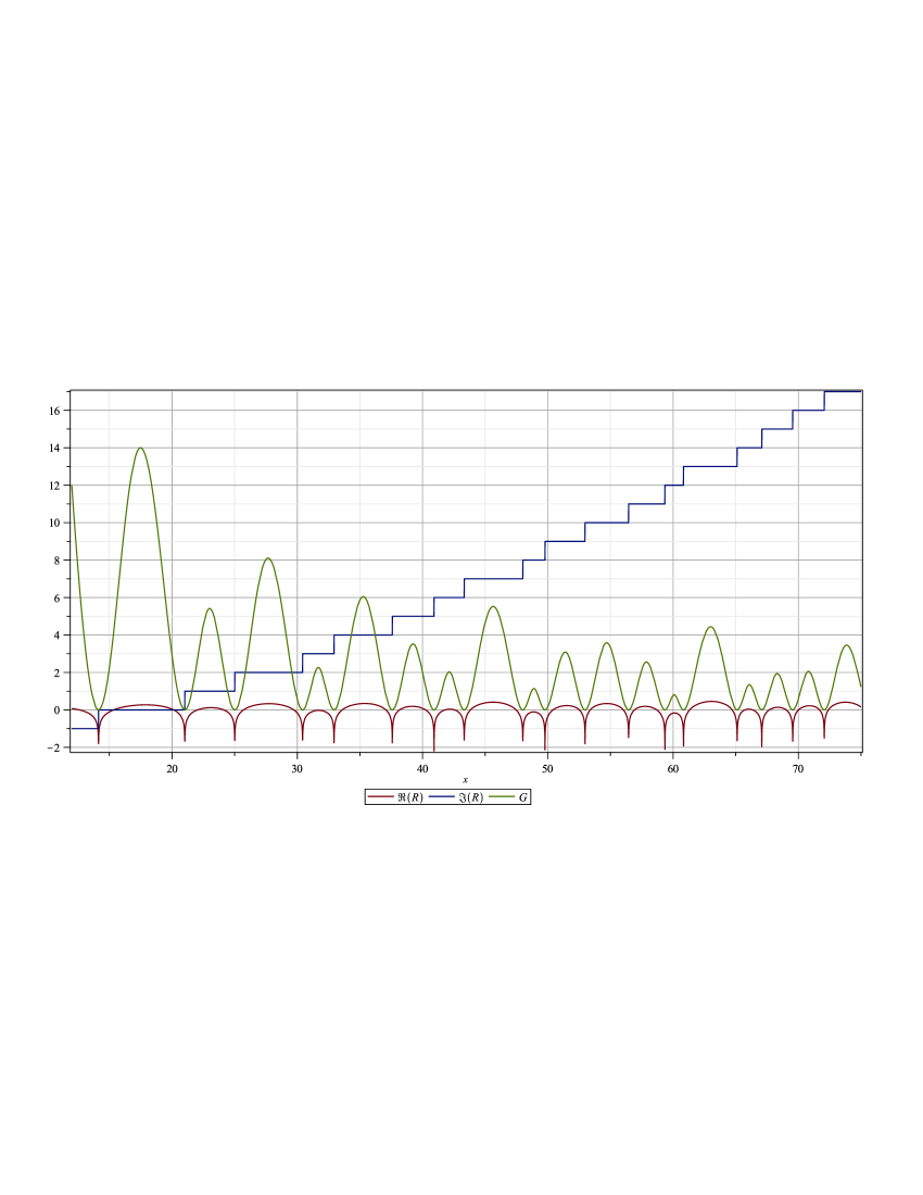
Figure 1: The Real and Imaginary Parts of $R(t)$ compared with $G(t)$

Now, let $H(t)$ be the derivative of $G(t)$ given by

$$\begin{array}[]{ll}H(t)&=\dot{G}(t)\\ &=\frac{\mathrm{d}}{\mathrm{d}t}\left(-\frac{1}{\Delta R(t)}\right)\\ &=-4i\pi z(t)\frac{z(t)^{3}\Delta g(t)+8(2z(t)^{2}\dddot{z}(t)-6z(t)\dot{z}(t)\ddot{z}(t)-4\dot{z}(t)^{3})}{(z(t)^{2}+8(z(t)\ddot{z}(t)-\dot{z}(t)^{2}))^{2}}\end{array}$$ (18)

When $H(t)=0$ and $\dot{H}(t)=\ddot{G}(t)=\Delta G(t)>0$, the point $t$ marks a minimum of $G(t)$ where it coincides with a Riemann zero, i.e., $\zeta\left(\frac{1}{2}+it\right)=0$, otherwise when $H(t)=0$ and $\dot{H}(t)=\Delta G(t)<0$, the point $t$ marks a local maximum $G(t)$, marking midway points between consecutive minima.

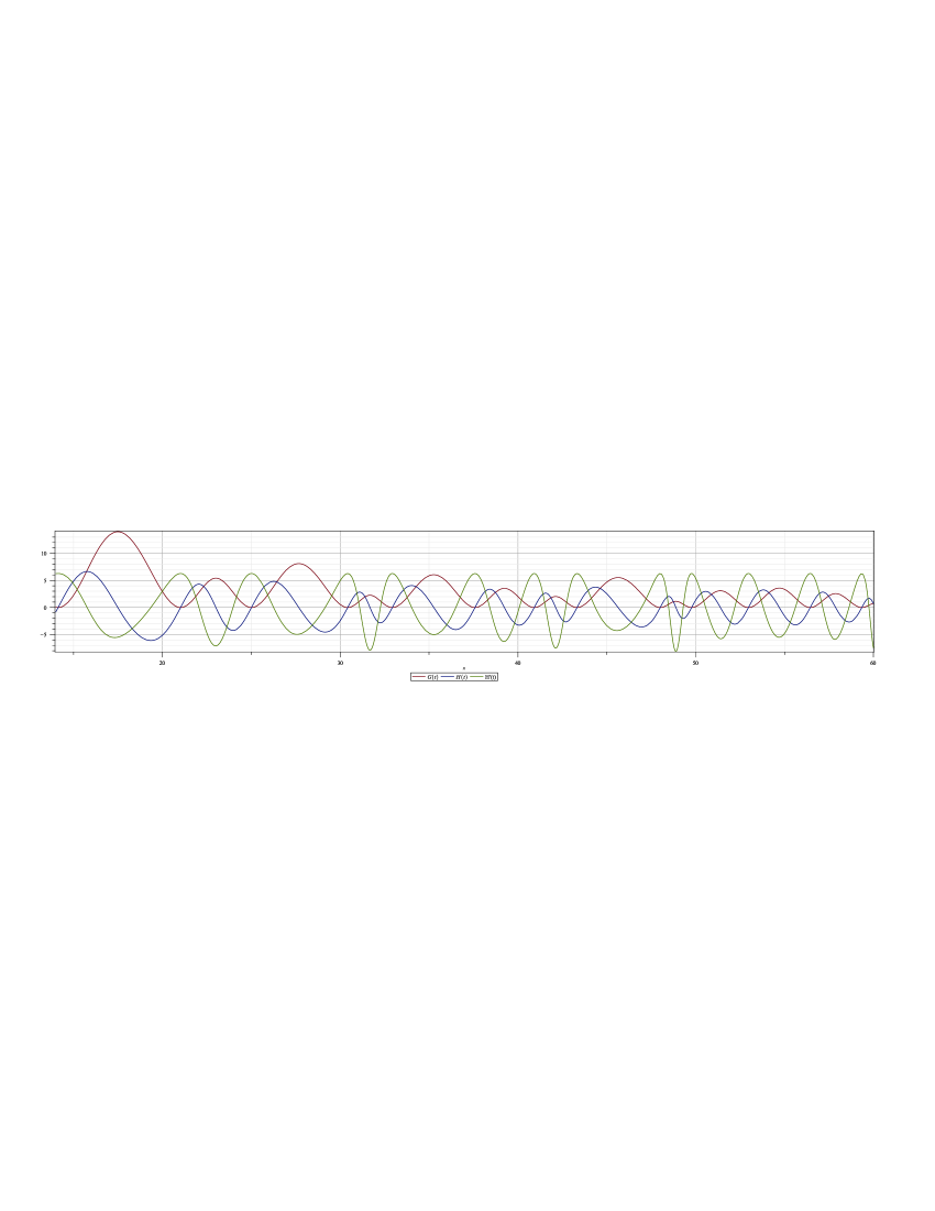
Figure 2: $G(t),H(t)\operatorname{and}\dot{H}(t)$

With the identity $t=\frac{1}{2}+i\left(\frac{i}{2}-it\right)$, define $\nu(t)$ as the Mobius transform of the partition function

$$\nu(t)=-\left(\Delta R\left(\frac{i}{2}-it\right)\right)^{-1}=-G\left(\frac{i}{2}-it\right)$$ (19)

then $\nu(t)$ has zeros at the positive odd integers, zero, and negative even integers. In the same way, let

$$\begin{array}[]{ll}\chi(t)&=\dot{\nu}(t)\\ &=-iH\left(\frac{i}{2}-it\right)\\ &=-4i\pi\zeta(t)\frac{\zeta(t)^{3}\left(\ddot{\Psi}\left(\frac{t}{2}\right)-\ddot{\Psi}\left(\frac{1}{2}-\frac{t}{2}\right)\right)-8(6\zeta(t)\dot{\zeta}(t)\ddot{\zeta}(t)+2\zeta(t)^{{}^{2}}\dddot{\zeta}(t)+4\dot{\zeta}(t)^{3})}{\zeta(t)^{2}\left(\left(\dot{\Psi}\left(\frac{t}{2}\right)-\dot{\Psi}\left(\frac{1}{2}-\frac{t}{2}\right)\right)+8(\zeta(t)\ddot{\zeta}(t)-\dot{\zeta}(t)^{2})\right)^{2}}\end{array}$$ (20)

which also has zeros on the real line at the positive odd integers, zero, and the negative even integers.

$$\begin{array}[]{rll}\lim_{t\rightarrow 2n-1}\nu(t)&=\lim_{t\rightarrow 2n-1}\chi(t)&=0\forall n>0\\ \lim_{t\rightarrow 0}\nu(t)&=\lim_{t\rightarrow 0}\chi(t)&=0\\ \lim_{t\rightarrow-2n}\nu(t)&=\lim_{t\rightarrow-2n}\chi(t)&=0\forall n<0\end{array}$$ (21)

Both $\nu(t)$ and $\chi(t)$ satisify similiar functional equations

$$\nu(t)=\nu(1-t)$$ (22)

and

$$\chi(t)=-\chi(1-t)$$ (23)

So the even $\mu(t)$ and odd $\psi(t)$ transcendental entire functions can be defined

$$\mu(t)=\nu\left(t+\frac{1}{2}\right)$$ (24)

$$\psi(t)=\chi\left(t+\frac{1}{2}\right)$$ (25)

which satisify the functional symmetries

$$\mu(t)=\mu(-t)$$ (26)

and

$$\psi(t)=-\psi(-t)$$ (27)

The function $\chi(t)$ has as a subset of its roots, the roots of the Rieman zeta function $\zeta(t)$, the converse is not true, since $\chi(t)$ is a function of $\zeta(t)$ and its first, second, and third derivatives.

$$\{t:\zeta(t)=0\}\subset\{t:\chi(t)=0\}$$ (28)

Let

$$\chi_{n}(t)=\chi(1+2n+2t)$$ (29)

and

$$\nu_{n}(t)=\nu(1+2n+2t)$$ (30)

which both satisify the symmetries

$$\chi_{-\frac{1}{2}}\left(\frac{t}{2}\right)=\chi(t)$$ (31)

$$\nu_{-\frac{1}{2}}\left(\frac{t}{2}\right)=\nu(t)$$ (32)

as well as

$$\chi_{n}\left(-\frac{1}{2}\right)=\chi(2n)$$ (33)

$$\nu_{{}_{n}}\left(-\frac{1}{2}\right)=\nu(2n)$$ (34)

The sequence of wave functions $\nu_{n}(t)$ converges, thanks to quantum ergodicity, to

$$\nu_{\infty}(t)=\lim_{n\rightarrow\infty}\nu_{n}(t)=\sin^{2}(\pi t)$$ (35)

which has a limiting maximum

$$\begin{array}[]{ll}\lim_{n\rightarrow\infty}\max_{0<t<1}\nu_{n}(t)&=\max_{0<t<1}\nu_{\infty}(t)\\ &=\lim_{n\rightarrow\infty}\nu(2n)\\ &=\frac{8}{\pi}\\ &\cong 2.546479089470\ldots\end{array}$$ (36)

and the associated differential is

$$\begin{array}[]{cl}\chi_{\infty}(t)&=\lim_{n\rightarrow\infty}\chi_{n}(t)\\ &=\frac{4}{\pi}\frac{\mathrm{d}}{\mathrm{d}t}\nu_{\infty}(t)\\ &=\frac{4}{\pi}\frac{\mathrm{d}}{\mathrm{d}t}\sin^{2}(\pi t)\\ &=-8\sin(\pi t)\cos(\pi t)\end{array}$$ (37)

It is worth mentioning that the pair-correlation function for the zeros of $\zeta(s)$ is

$$r_{2}(x)=1-\frac{\sin^{2}(\pi x)^{2}}{\pi^{2}x^{2}}$$

if the Riemann hypothesis is true. [11] The point $n=1$ is where $\chi_{n}\left(-\frac{1}{2}\right)$ and $\nu_{n}\left(-\frac{1}{2}\right)$ attain their greatest values among the integers.

$n$	$\nu_{n}\left(-\frac{1}{2}\right)$	$\chi_{n}\left(-\frac{1}{2}\right)$
$1$	117.43532857805377782	9447.7593604718560
$2$	003.03320654562255410	0000.2816402783351
$3$	002.77176105375846239	0000.0589526080385
$4$	002.69653220844944185	0000.0240373109008
5	002.66095375057354766	0000.0132398305603
$6$	002.63970550787458574	0000.0088555925215
$7$	002.62532107269483772	0000.0060558883634
…	$\ldots\ldots\ldots\ldots\ldots\ldots$	$\ldots\ldots\ldots\ldots\ldots\ldots\ldots$
$\infty$	$\frac{8}{\pi}$	0

Table 1: Even values of $\nu(n)$ and $\chi(n)$

This phenomena of having the first wave function having a much larger size than all of the remainders is mentioned in [Kna99, Theorem 22] The convergence of $\lim_{n\rightarrow\infty}\nu_{n}(t)\rightarrow\nu_{\infty}(t)$ and $\lim_{n\rightarrow\infty}\chi_{n}(t)\rightarrow\chi_{\infty}(t)$ might be interpreted as a manifestation of quantum ergodicity [11, C p.16]. There is an essential singularity[CB90, 54 p.169] at $s_{0}\cong 1.98757823\ldots$

$$\lim_{s\rightarrow s_{0}}\chi(s)=\infty$$ (38)

We also have the limits

$$\lim_{s\rightarrow\{0,1\}}\dot{\chi}(s)=4\pi$$ (39)

The integral over this sine-squared kernel is

$$\int_{0}^{1}\sin^{2}(\pi t)\mathrm{d}t=\frac{1}{2}$$ (40)

whereas

$$\frac{}{}\int_{0}^{1}\frac{\nu(t)}{\nu\left(\frac{1}{2}\right)}\mathrm{d}t\cong.46693755153559653755\ldots$$ (41)

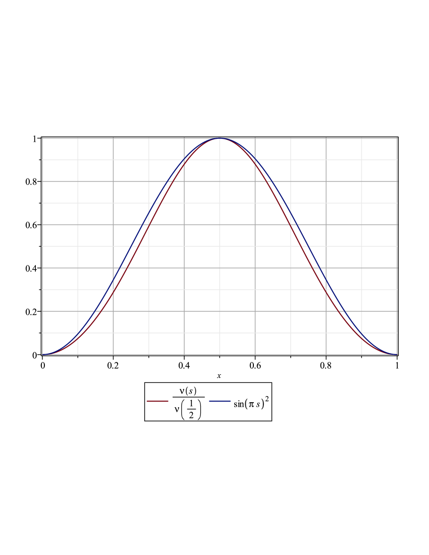
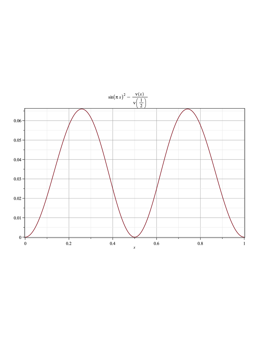
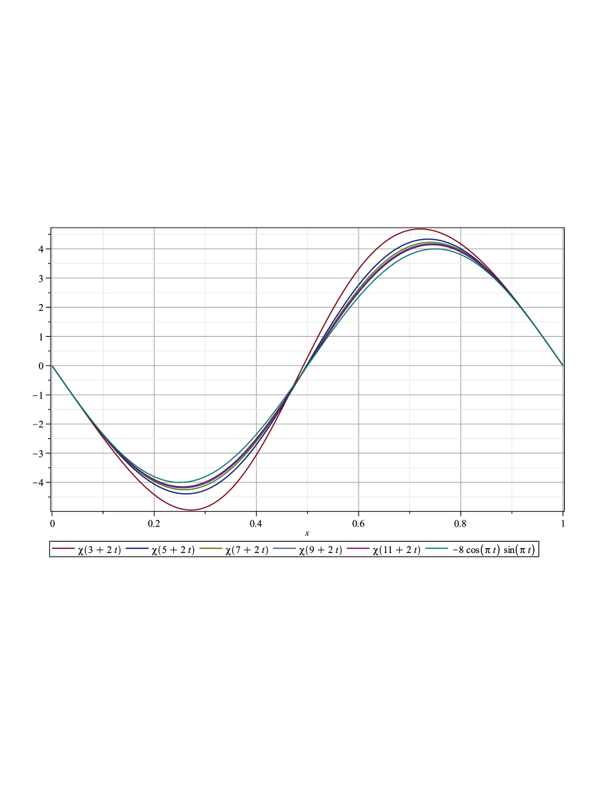
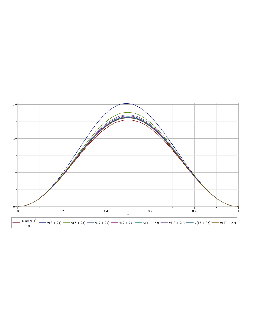
Figure 3: Top Left: The function $\nu(s)$ normalized by its maximum value on $[0,1]$ Top Right: The function $\nu(s)$ normalized by its maximum value and subtracted from $\sin^{2}(\pi x)$ Bottom Left: Convegence of $\chi_{n}(t)\rightarrow-8\cos(\pi t)\sin(\pi t)$  Bottom Right: Convegence of $\nu_{n}(t)\rightarrow\sin^{2}(\pi t)\frac{\pi}{8}$

2 Appendix

2.1 Wave Mechanics

2.2 The One-Dimensional Wave Equation

The one-dimensional wave equation is

$$-\frac{\hbar^{2}}{2m}\frac{\partial^{2}}{x^{2}}u(x,t)+V(x,t)u(t,x)=-\frac{\hbar}{i}\frac{\partial}{\partial t}u(x,t)$$ (42)

[Flü94, II.A.4 p.25][Gan06, 4.2.1 p.][Coo03, Ch. 8 p.147]

2.3 The Poisson Bracket and Lagrangian Mechanics

“The” Poisson bracket, expressed with Einstein summation convention (for the repeated index $i$)

$$\{A,B\}\equiv\frac{\partial A}{\partial p_{i}}\frac{\partial B}{\partial q_{i}}-\frac{\partial B}{\partial p_{i}}\frac{\partial A}{\partial q_{i}}$$ (43)

has the antisymmetry property

$$\{A,B\}=-\{B,A\}$$ (44)

and the so-called Jacobi identity

$$\{A,\{B,C\}\}-\{B,\{A,C\}\}+\{C,\{A,B\}\}=0$$ (45)

Two quantitities $A$ and $B$ are said to commute if their $\operatorname{Poisson}\operatorname{bracket}$ $\{A,B\}$ vanishes, that is, $\{A,B\}=0$. Hamilton’s equations of motion for the system

$$\dot{p}_{i}=-\frac{H}{q_{i}}$$ (46)

$$\dot{q}_{i}=\frac{\partial H}{\partial q_{i}}$$ (47)

where $H$ is a Legendre-transformed function of the Lagrangian called the Hamiltonian

$$H\equiv\frac{\partial L}{\partial\dot{q}_{i}}\dot{q}_{i}-L(q_{i},\dot{q}_{i},t)$$ (48)

whose value for any given time $t$ gives the energy

$$\mathcal{A}[q_{i}]=\int_{t_{a}}^{t_{b}}L(q_{i},\dot{q}_{i},t)\mathrm{d}t$$ (49)

of the system where $L(q_{i},\dot{q}_{i},t)$ is the Lagrangian of the system and

$$q_{i}(t)=q_{i}^{\operatorname{cl}}(t)+\delta q_{i}(t)$$ (50)

is an arbitrary path where $q_{i}^{\operatorname{cl}}(t)$ is the classical orbit or classical path of the system and

$$\delta q_{i}(t_{a})\equiv q_{i}(t)-q^{\operatorname{cl}}_{i}(t)$$ (51)

[Kle04, 1.1]

2.3.1 The Euler-Lagrange equation

The Euler-Lagrange equation

$$\frac{\mathrm{d}}{\mathrm{d}t}\left(\frac{\partial L}{\partial\dot{q}_{i}}\right)=\frac{\partial L}{\partial q_{i}}$$ (52)

indicates that the action $S$ given by

$$S=\int_{t_{1}}^{t_{2}}L(t)\mathrm{d}t$$ (53)

where

$$L(t)=T-V(x(t))$$ (54)

is the Lagrangian and

$$T(t)=\frac{1}{2}m\dot{x}(t)^{2}$$ (55)

is the kinetic energy  which is stationary for the physical solutions $q_{i}(t)$.[Gan06, 4.2.1]

2.3.2 Quantum Mechanics of General Lagrangian Systems

The coordinate transformation

$$x^{i}=x^{i}(q^{\mu})$$ (56)

implies the relation

$$\partial_{\mu}=\frac{\partial}{\partial q^{\mu}}=e^{i}_{\mu}(q)\partial_{i}$$ (57)

between the derivatives $\partial_{\mu}$ and

$$\partial_{i}\equiv\frac{\partial}{\partial x^{i}}$$ (58)

where

$$e^{i}_{\mu}(q)\equiv\partial_{\mu}x^{i}(q)$$ (59)

is a transformation matrix called the basis p-ad where $p$ is the prefix corresponding to $n$, the dimension of $x$, monad when $n=1$, dyad when $n=2$, triad when $n=$3, and so on. Let

$$e_{i}^{\mu}(q)=\frac{\partial q^{\mu}}{\partial x^{i}}$$ (60)

be the inverse matrix called the reciprocal p-ad. The $\operatorname{basis}p-\operatorname{ad}$ and its recpiprocal satisify the orthogonality and completeness relations

$$e^{i}_{\mu}e_{i}^{\nu}=\delta_{\mu}^{\nu}$$ (61)

and

$$e_{\mu}^{i}e_{j}^{\mu}=\delta_{j}^{i}$$ (62)

The inverse of $\partial_{\mu}$ is

$$\partial_{i}=e_{i}^{\mu}(q)\partial_{\mu}$$ (63)

which is related to the curvilinear transform of the Cartesian quantum-mechanical momentum operators by

$$\hat{p}_{i}=-i\hbar\partial_{i}=-i\hbar e_{i}^{\mu}(q)\partial_{\mu}$$ (64)

The Hamiltonian operator for free particles is defined by

$$\hat{H}_{0}=\hat{T}=\frac{1}{2M}\hat{p}^{2}=-\frac{\hbar^{2}}{2M}\Delta$$ (65)

where its metric tensor is given by

$$g^{\mu\nu}(q)\equiv e^{\mu}_{i}(q)e^{\nu}_{i}(q)$$ (66)

and its inverse by

$$g_{\mu\nu}(q)\equiv e^{i}_{\mu}(q)e^{i}_{\nu}(q)$$ (67)

The Laplacian of a metric tensor is then expressed

$$\begin{array}[]{ll}\Delta&=\partial_{i}^{2}\\ &=e^{i\mu}\partial_{\mu}e^{i\nu}\partial_{\nu}\\ &=e^{i\mu}e^{i\nu}\partial_{\mu}\partial_{\nu}+(e^{i\mu}\partial_{\mu}e^{i\nu})\partial_{\nu}\\ &=g^{\mu\nu}(q)\partial_{\mu}\partial_{\nu}-\Gamma_{\mu}^{\mu\nu}(q)\partial_{\nu}\end{array}$$ (68)

where

$$\Gamma_{\mu\nu}^{\lambda}(q)=-e^{i}_{v}(q)\partial_{\mu}e_{i}^{\lambda}(q)=e_{i}^{\lambda}(q)\partial_{u}e^{i}_{\nu}(q)$$ (69)

is the affine-connection [Kle04, 1.13][Pod28]

2.3.3 Noether’s Theorem and Lie Groups

From Noether’s theorem it is known that continuous symmetries have corresponding conservation laws.[Gan06, 4.2.1] Let

$$\alpha_{s}$$ (70)

be a continuous family of symmetries which is a $1$-parameter subgroup $s\mapsto\alpha_{s}$ in the Lie group of symmetries. A Lie group is a group whose operations are compatible with the smooth structure. A smooth structure on a manifold allows for an unambiguous notion of smooth function.

2.4 Schroedinger’s Time-Dependent Equation and Nonstationary Wave Motion

The function $\cos^{2}(t)=1-\sin^{2}(t)$ arises in the Dirac phase averaving method of calculating transition probabilities of non-stationary states in the time-dependent Schroedinger equation. [Gol61, 15.1] 3

2.4.1 Operators and Observables: Dirac’s Time-Dependent Theory

Let

$$y(x,t)=A\cos\left(\frac{2\pi px}{h}\right)\cos\left(\frac{2\pi\epsilon t}{h}\right)$$

where

$$\epsilon=hv$$ (71)

which relates the energies of a “matter wave” system, whatever that is, maybe a fermionic system, to the frequencies of quanta it emits or absorbs. There is always some arbitriness with choice of units. This wave function has the symmetry

$$\frac{\partial^{2}y(x,t)}{x^{2}}=-\left(\frac{2\pi}{h}\right)^{2}p^{2}y(x,t)$$ (72)

so that the kinetic energy of a particle is obtained from the wave function

$$-\frac{(2\pi)^{2}}{2m}\frac{\partial^{2}y(x,t)}{x^{2}}=\frac{p^{2}}{2m}y(x,t)$$ (73)

which means formally that

$$\frac{1}{2m}(p)^{2}y(x,t)=-\frac{1}{2m}\left(\frac{2\pi}{i}\frac{\partial}{\partial x}\right)^{2}$$ (74)

which suggests the identifiation of the Schroedinger momentum operator

$$\left(\frac{2\pi}{i}\frac{\partial}{\partial x}\right)\leftrightarrow p$$ (75)

The equation for “nonfree” particles is augmented by

$$\frac{m}{2}\left(\frac{2\pi}{i}\frac{\partial}{\partial x}\right)^{2}y(x,t)=[\epsilon-V(x)]y(x,t)$$ (76)

where $\epsilon$ is the total energy of the particle and $V(x)$ is its potential energy. The first Schroedinger equation is then expressed

$$\epsilon y(x,t)=\left[\frac{1}{2m}\left(\frac{2\pi}{i}\frac{\partial}{\partial x}\right)^{2}+V(x)\right]y(x,t)=\left[\frac{1}{2m}(p)^{2}+V(x)\right]y(x,t)$$ (77)

or

$$H_{y(x,t)}=\epsilon y(x,t)$$

where $H$ is the operator corresponding to the Hamiltonian of the (point) particle. [Gol61, 11.5] The time-dependent Schroedinger equation is written

$$\frac{\partial^{2}(x,t)}{\partial t^{2}}=-\frac{1}{(2\pi)^{2}}\epsilon^{2}y(x,t)=-\left(\frac{H}{2\pi}\right)^{2}y(x,t)$$ (78)

or equivalently as

$$0=\left((2\pi)^{2}\frac{\partial^{2}}{\partial t^{2}}+H^{2}\right)y(x,t)=\left(H+i2\pi\frac{\partial}{\partial t}\right)\left(H-i2\pi\frac{\partial}{\partial t}\right)y(x,t)$$ (79)

where

$$Hy(x,t)=i2\pi\frac{\partial}{\partial t}y(x,t)$$ (80)

It is also worth mentioning that in Dirac’s theory of the time-dependent Schroedinger there is a Hamiltonian of the form

$$H=H_{0}+\lambda H_{1}(t)$$ (81)

which has a transition probability per unit time of

$$w(p\rightarrow-p)=\frac{V_{0}^{2}\sin^{2}\left(2l\sqrt{\frac{2m\epsilon}{{}^{\hbar^{2}}}}\right)}{2\sqrt{8m}\epsilon^{\frac{3}{2}}L}$$

where $V_{0},\epsilon,h,\operatorname{and}L$ are suitable constants. [Gol61, 15.5]

2.4.2 The String Theoretic Partition Function

The string theoretic partition function is defined as

$$Z_{st}(\omega)=Z_{st,R}(\omega)=\operatorname{Tr}[e^{2\pi i\omega_{1}P-2\pi\omega_{2}H}]=(q\bar{q})^{-\frac{1}{24}}\operatorname{Tr}(q^{L_{0}^{+}}\bar{q}^{L^{-}_{0}})$$ (82)

where $L^{+}_{0}$ and $L^{-}_{0}$ are the Virasoro generators defined by

$$L_{0}^{\pm}=\frac{(p^{+})^{2}+(p^{-})^{2}}{2}+\sum_{n=1}^{\infty}\alpha_{-n}^{\pm}\alpha_{n}^{\pm}$$ (83)

and $\alpha_{-n}^{\pm}\alpha_{n}$ are related to something called a Fubini-Veneziano field and $p^{{}_{+}}$ is the left-momentum operator and $p^{-}$ is right-momentum operator. [Lap08, 2.2.1]

References

- [11] D. Schumayer and D. A. W. Hutchinson. Colloquium: Physics of the Riemann hypothesis. Reviews of Modern Physics, 83:307–330, apr 2011.
- [CB90] Ruel V. Churchill and James Ward Brown. Complex Variables and Applications. McGraw-Hill Publishing Company, 1990.
- [Coo03] David B. Cook. Probability and Schrodinger’s Mechanics. World Scientific Publishing Company, 2003.
- [Flü94] S. Flügge. Practical Quantum Mechanics. Classics in Mathematics. Springer Berlin Heidelberg, 1994.
- [Gan06] Terry Gannon. Moonshine Beyond the Monster: The Bridge Connecting Algebra, Modular Forms, and Physics. Cambridge University Press, Monographs on Mathematical Physics, 2006.
- [Gol61] Sydney Golden. An Introduction to Theoretical Physical Chemistry. Series In Chemistry. Addison-Wesley Publishing Company, Inc., 1961.
- [Ivi13] A. Ivić. The Theory of Hardy’s Z-Function. Cambridge Tracts in Mathematics. Cambridge University Press, 2013.
- [Kle04] H. Kleinert. Path Integrals in Quantum Mechanics, Statistics, Polymer Physics, and Financial Markets. World Scientific, 2004.
- [Kna99] Andreas Knauf. Number theory, dynamical systems and statistical mechanics. Reviews in Mathematical Physics, 11(08):1027–1060, 1999.
- [Lap08] Michel L. Lapidus. In search of the Riemann zeros: Strings, Fractal membranes and Noncommutative Spacetimes. American Mathematical Society, 2008.
- [Pod28] Boris Podolsky. Quantum-mechanically correct form of hamiltonian function for conservative systems. Phys. Rev., 32:812–816, Nov 1928.