Rôle of the pion electromagnetic form factor in the $\Delta(1232)\to\gamma^{\ast}N$
timelike transition

Abstract

The $\Delta(1232)\to\gamma^{\ast}N$ magnetic dipole form factor ($G_{M}^{\ast}$) is described here within a new covariant model that combines the valence quark core together with the pion cloud contributions. The pion cloud term is parameterized by two terms: one connected to the pion electromagnetic form factor, the other to the photon interaction with intermediate baryon states. The model can be used in studies of pp and heavy ion collisions. In the timelike region this new model improves the results obtained with a constant form factor model fixed at its value at zero momentum transfer. At the same time, and in contrast to the Iachello model, this new model predicts a peak for the transition form factor at the expected position, i.e. at the $\rho$ mass pole. We calculate the decay of the $\Delta\to\gamma N$ transition, the Dalitz decay ($\Delta\to e^{+}e^{-}N$), and the $\Delta$ mass distribution function. The impact of the model on dilepton spectra in pp collisions is also discussed.

I Introduction

To understand the structure of hadrons, baryons in particular, in terms of quarks and gluons at low energies, is theoretically challenging due to the intricate combination of confinement and spontaneous chiral symmetry breaking, and the non-perturbative character of QCD in that energy regime. Fortunately, experimentally electromagnetic and hadron beams in accelerator facilities are decisive tools to reveal that structure, and seem to indicate a picture where effective degrees of freedom as baryon quark cores dressed by clouds of mesons play an important role. For a review on these issues see NSTAR . Although different, experiments with electromagnetic and strong probes complement each other. In electron scattering, virtual photons disclose the region of momentum transfer $q^{2}<0$, and spacelike form factors are obtained NSTAR ; MesonBeams ; HADES14 . Scattering experiments of pions or nucleons with nucleon targets involving Dalitz decays of baryon resonances MesonBeams ; Timelike ; HADES14 ; Frohlich10 provide information on timelike form factors, defined in the $q^{2}>0$ region where the meson spectrum arises. The results of all these different measurements have to match at the photon point ($q^{2}=0$).

Among the several baryon resonances the $\Delta$ excitation and decays have a special role and are not yet fully understood. The electromagnetic transition between the nucleon and the $\Delta(1232)$, and in particular its dominant magnetic dipole form factor $G_{M}^{\ast}(q^{2})$, as function of $q^{2}$, is a prime example that discloses the complexity of the electromagnetic structure of the excited states of the nucleon and illustrates the limitations of taking into account only valence quark degrees of freedom for the description of the transition.

In the region of small momentum transfer $G_{M}^{\ast}(q^{2})$ is usually underestimated by valence quark contributions alone. Several models have been proposed in order to interpret this finding. Most of them are based on the interplay between valence quark degrees of freedom and the so-called meson cloud effects, in particular, the dominant pion cloud contribution NSTAR ; NDelta ; NDeltaD ; LatticeD ; Octet2Decuplet ; Octet2Decuplet2 ; DynamicalModels . Other recent works on the $\Delta\to\gamma^{\ast}N$ transition can be found in Refs. Braun06 ; Alexandrou11 ; Eichmann12 ; Segovia14 .

In this work we propose a hybrid model which combines the valence quark component, determined by a constituent quark model, constrained by lattice QCD and indirectly by experimental data, with a pion cloud component. The pion cloud component is written in terms of the pion electromagnetic form factor and therefore constrained by data.

The $\Delta\to\gamma^{\ast}N$ transition in the timelike region was studied using vector meson dominance (VMD) models Schafer94b ; deJong96 ; Krivoruchenko02 ; Faessler03 , the constant form factor model Zetenyi03 ; Frohlich10 , a two component model (model with valence quark and meson cloud decomposition), hereafter called the Iachello model Frohlich10 ; Iachello ; Iachello73 , and the covariant spectator quark model Timelike (which incidentally also assumes VMD for the quark electromagnetic current).

The Iachello model pioneered the timelike region studies of the $\Delta\to\gamma^{\ast}N$ transition. The model was successful in the description of the nucleon form factors Iachello73 but has been criticized for generating the pole associated with the $\rho$-meson pole near $q^{2}\simeq 0.3$ GeV², below $q^{2}=m_{\rho}^{2}\simeq 0.6\;\mathrm{GeV}^{2}$ Frohlich10 as it should. The constant form factor model is a good starting point very close to $q^{2}=0$ but, on the other hand, does not satisfactorily take into account the finite size of the baryons and their structure of non-pointlike particles.

In the covariant spectator quark model the contributions for the transition form factors can be separated into valence quark and meson cloud effects (dominated by the pion). The valence quark component is directly constrained by lattice QCD data, and has been seen to coincide with the valence quark core contributions obtained from an extensive data analysis of pion photo-production Lattice ; LatticeD ; EBAC . Its comparison to experimental data enables the extraction of information on the complementary meson cloud component in the spacelike region Timelike ; NDelta . However the extension to the timelike region of the meson cloud is problematic given the difficulty of a calculation that comprises also in a consistent way the whole meson spectrum. In Ref. Timelike the meson cloud was parameterized by a function $F_{\rho}$, taken from the Iachello model where it describes the dressing of the $\rho$-propagator by intermediate $\pi\pi$ states. As noted before, unfortunately, the function $F_{\rho}$ has a peak that is displaced relatively to the $\rho$-meson pole mass. Here, by directly using the pion form factor data we corrected for this deficiency.

Figure 1: Pion cloud contributions for the $\Delta\to\gamma^{\ast}N$ electromagnetic transition form factors. Between the initial and final state there are several possible intermediate octet baryon and/or decuplet baryon states: $B_{1}$ in diagram (a); $B_{2}$ and $B_{3}$ in diagram (b).

Moreover, in previous works Timelike ; NDelta ; NDeltaD ; LatticeD ; Octet2Decuplet we have assumed that the pion cloud contributions for the magnetic dipole form factor could be represented by a simple parameterization of one term only. But in the present work we introduce an alternative parameterization of the pion cloud which contains two terms. These two leading order contributions for the pion cloud correspond to the two diagrams of Fig. 1. We use then a parameterization of the pion cloud contributions for $G_{M}^{\ast}$ where diagram (a) is related to the pion electromagnetic form factor $F_{\pi}(q^{2})$, and is separated from diagram (b). Diagram (a), where the photon couples directly to the pion, is dominant according to chiral perturbation theory, which is valid in the limit of massless and structureless quarks. But the other contribution, from diagram (b), where the photon couples to intermediate (octet or decuplet) baryon states while the pion is exchanged between those states, becomes relevant in models with constituent quarks with dressed masses and non-zero anomalous magnetic moments. This was shown in Ref. Octet2Decuplet2 on the study of the meson cloud contributions to the magnetic dipole moments of the octet to decuplet transitions. The results obtained for the $\Delta\to\gamma^{\ast}N$ transition in particular, suggests that both diagrams contribute with almost an equal weight.

II Iachello model

In the Iachello model the dominant contribution to the $\Delta\to\gamma^{\ast}N$ magnetic dipole form factor is the meson cloud component (99.7%) Frohlich10 . The meson cloud contributions is estimated by VMD in terms of a function $F_{\rho}$ from the dressed $\rho$ propagator, which in the limit $q^{2}\gg 4m_{\pi}^{2}$, reads Timelike

$$\begin{split}F_{\rho}(q^{2})&=\frac{m_{\rho}^{2}}{m_{\rho}^{2}-q^{2}-\frac{1}{\pi}\frac{\Gamma_{\rho}^{0}}{m_{\pi}}q^{2}\log\frac{q^{2}}{m_{\pi}^{2}}+i\frac{\Gamma_{\rho}^{0}}{m_{\pi}}q^{2}},\\ &=\frac{m_{\rho}^{2}}{m_{\rho}^{2}+Q^{2}+\frac{1}{\pi}\frac{\Gamma_{\rho}^{0}}{m_{\pi}}Q^{2}\log\frac{Q^{2}}{m_{\pi}^{2}}}.\end{split}$$ (1)

In the previous equation $Q^{2}=-q^{2}$, $m_{\pi}$ is the pion mass, and $\Gamma_{\rho}^{0}$ is a parameter that can be fixed by the experimental $\rho$ decay width into $2\pi$, $\Gamma_{\rho}^{0}=0.149$ GeV or $\Gamma_{\rho}^{0}=0.112$ GeV depending on the specific model Timelike ; Iachello .

III Covariant spectator quark model

Within the covariant spectator quark model framework the nucleon and the $\Delta$ are dominated by the $S$-wave components of the quark-diquark configuration Nucleon ; NDelta ; Nucleon2 . In this case the only non-vanishing form factor of the $\Delta\to\gamma^{\ast}N$ transition is the magnetic dipole form factor, which anyway dominates in all circumstances.

One can then write NDelta ; NDeltaD ; LatticeD

$$G_{M}^{\ast}(q^{2},W)=G_{M}^{B}(q^{2},W)+G_{M}^{\pi}(q^{2}),$$ (2)

where $G_{M}^{B}$ is the contribution from the bare core and $G_{M}^{\pi}$ the contribution of the pion cloud. Here $W$ generalizes the $\Delta$ mass $M_{\Delta}$ to an arbitrary invariant mass $W$ in the intermediate states Timelike . We omitted the argument $W$ on $G_{M}^{\pi}$ since we take that function to be independent of $W$.

Following Refs. NDelta ; NDeltaD ; LatticeD ; Timelike we can write

$$G_{M}^{B}(q^{2},W)=\frac{8}{3\sqrt{3}}\frac{M}{M+W}f_{v}(q^{2}){\cal I}(q^{2},W),$$ (3)

where

$${\cal I}(q^{2},W)=\int_{k}\psi_{\Delta}(P_{+},k)\psi_{N}(P_{-},k),$$ (4)

is the overlap integral of the nucleon and the $\Delta$ radial wave functions which depend on the nucleon ($P_{-}$), the Delta ($P_{+}$) and the intermediate diquark ($k$) momenta. The integration symbol indicates the covariant integration over the diquark on-shell momentum. For details see Refs. NDelta ; Timelike .

As for $f_{v}(q^{2})$ it is given by

$$f_{v}(q^{2})=f_{1-}(q^{2})+\frac{W+M}{2M}f_{2-}(q^{2})$$ (5)

where $f_{i-}$ ($i=1,2$) are the quark isovector form factors that parameterize the electromagnetic photon-quark coupling. The form of this parameterization assumes VMD mechanism Nucleon ; NDelta ; Omega . See details in Appendix A.

In this work we write the pion cloud contribution as

$$G_{M}^{\pi}(q^{2})=3\frac{\lambda_{\pi}}{2}\left[F_{\pi}(q^{2})\left(\frac{\Lambda_{\pi}^{2}}{\Lambda_{\pi}^{2}-q^{2}}\right)^{2}+\tilde{G}_{D}^{2}(q^{2})\right],$$ (6)

where $\lambda_{\pi}$ is a parameter that define the strength of the pion cloud contributions, $F_{\pi}(q^{2})$ is a parameterization of the pion electromagnetic form factor and $\Lambda_{\pi}$ is the cutoff of the pion cloud component from diagram (a). The function $\tilde{G}_{D}^{2}$ on Eq. (6) simulates the contributions from the diagram (b), and therefore includes the contributions from several intermediate electromagnetic transitions between octet and/or decuplet baryon states.

From perturbative QCD arguments it is expected that the latter effects fall off with $1/Q^{8}$ Carlson . At high $Q^{2}$ a baryon-meson system can be interpreted as a system with $N=5$ constituents, which produces transition form factors dominated by the contributions of the order $1/(Q^{2})^{(N-1)}=1/Q^{8}$. This falloff power law motivates our choice for the form of $\tilde{G}_{D}^{2}$: the timelike generalization of a dipole form factor $G_{D}=\left(\frac{\Lambda_{D}^{2}}{\Lambda_{D}^{2}-q^{2}}\right)^{2}$, where $\Lambda_{D}$ is a cutoff parameter defining the mass scale of the intermediate baryons.

The equal relative weight of the two terms of Eq. (6), given by the factor $\frac{1}{2}\lambda_{\pi}$, was motivated by the results from Ref. Octet2Decuplet2 , where it was shown that the contribution from each diagram (a) and (b) for the total pion cloud in the $\Delta\to\gamma^{\ast}N$ transition is about 50%. The overall factor 3 was included for convenience, such that in the limit $q^{2}=0$ one has $G_{M}^{\pi}(0)=3\lambda_{\pi}$. Since $G_{M}^{\ast}(0)\simeq 3$, $\lambda_{\pi}$ represents the fraction of the pion cloud contribution to $G_{M}^{\ast}(0)$.

In the spacelike regime, in order to describe the valence quark behavior ($1/Q^{4}$) of the form factors associated with the nucleon and $\Delta$ baryons, the dipole form factor $G_{D}$ with a cutoff squared value $\Lambda_{D}^{2}=0.71\,\mathrm{GeV}^{2}$ had been used in previous works Nucleon ; NDelta . As we will show, a model with $\Lambda_{D}^{2}=0.71\,\mathrm{GeV}^{2}$ provides a very good description of the $\Delta\to\gamma^{\ast}N$ form factor data in the region $-2\,\mathrm{GeV}^{2}<q^{2}<0$. However, since in the present work we are focused on the timelike region, we investigate the possibility of using a larger value for $\Lambda_{D}^{2}$, such that the effects of heavier resonances ($\Lambda_{D}^{2}\approx 1\,\mathrm{GeV}^{2}$) can also be taken into account.

To generalize $G_{D}$ to the timelike region we define $\tilde{G}_{D}(q^{2})$

$$\tilde{G}_{D}(q^{2})=\frac{\Lambda_{D}^{4}}{(\Lambda_{D}^{2}-q^{2})^{2}+\Lambda_{D}^{2}\Gamma_{D}^{2}},$$ (7)

where $\Gamma_{D}(q^{2})$ is an effective width discussed in Appendix B, introduced to avoid the pole $q^{2}=\Lambda_{D}^{2}$. Since $\Gamma_{D}(0)=0$, in the limit $q^{2}=0$, we recover the spacelike limit $\tilde{G}_{D}(0)=G_{D}(0)=1$. We note that differently from the previous work Timelike $\tilde{G}_{D}$ is the absolute value of $G_{D}$, and not its real and imaginary parts together.

To summarize this Section: Eq. (6) modifies the expression of the pion cloud contribution from our previous works, by including an explicit term for diagram (b) of Fig. 1. Diagram (a) is calculated from the pion form factor experimental data. Diagram (b) concerns less known phenomenological input. The $q^{2}$ dependence of that component is modeled by a dipole function squared. Since $\lambda_{\pi}$ was fixed already by the low $q^{2}$ data, in the spacelike region, the pion cloud contribution is defined only by the two cutoff parameters $\Lambda_{\pi}$ and $\Lambda_{D}$.

Next we discuss the parameterization of the pion electromagnetic form factor $F_{\pi}(q^{2})$, which fixes the term for diagram (a) and is known experimentally.

IV Parameterization of $F_{\pi}(q^{2})$

The data associated with the pion electromagnetic form factor $F_{\pi}(q^{2})$ is taken from the $e^{+}e^{-}\to\pi^{+}\pi^{-}$ cross-section (the sign of $F_{\pi}(q^{2})$ is not determined).

The function $F_{\pi}(q^{2})$ is well described by a simple monopole form as $F_{\pi}(q^{2})=\frac{\alpha}{\alpha-q^{2}-i\beta}$, where $\alpha$ is a cutoff squared and $\beta$ is proportional to a constant width. An alternative expression for $F_{\pi}(q^{2})$, that replaces the Iachello form $F_{\rho}$ is,

$$F_{\pi}(q^{2})=\frac{\alpha}{\alpha-q^{2}-\frac{1}{\pi}\beta q^{2}\log\frac{q^{2}}{m_{\pi}^{2}}+i\beta q^{2}}.$$ (8)

Eq. (8) simulates the effect of the $\rho$ pole with an effective width regulated by the parameter $\beta$. Note that also Eq. (8) has a form similar to the function $F_{\rho}$ of the Iachello model given by Eq. (1). In particular, when $\alpha\to m_{\rho}^{2}$ and $\beta\to\frac{\Gamma_{\rho}^{0}}{m_{\pi}}$, we recover Eq. (1). The advantage of Eq. (8) over Eq. (1) is that $\alpha$ and $\beta$ can be adjusted independently to the $|F_{\pi}|^{2}$ data. The result for those parameters from the fit in both time- and spacelike regions gives

$$\alpha=0.696\;\mbox{GeV}^{2},\hskip 19.91684pt\beta=0.178.$$ (9)

In the Iachello model (1) one has $\beta\simeq 1.1$, a very different value. The fit is illustrated in Fig 2. The best fit selects $\alpha\simeq 0.7\,\mathrm{GeV}^{2}$, which is larger than $m_{\rho}^{2}\simeq 0.6\,\mathrm{GeV}^{2}$. However, in the best fit to the data, the value of $\alpha$ is corrected by the logarithmic counterterm in the denominator of Eq. (8), that pushes the maximum of $|F_{\pi}(q^{2})|^{2}$ to the correct position, $q^{2}\simeq 0.6$ GeV². In the Iachello model, since $\beta\simeq 1.1$, the correction is too strong, and the maximum moves to $q^{2}\simeq 0.3$ GeV², differing significantly from the $|F_{\pi}(q^{2})|^{2}$ data.

To describe the physics associated with the $\rho$-meson, we restricted the fit to $q^{2}<0.6\,\mathrm{GeV}^{2}$, which causes a less perfect description of $F_{\pi}$ at the right side of the peak. However increasing $q^{2}$ beyond that point slightly worsens the fit. This probably indicates that although the $\omega$ width is small, there may be some interference from the ${\omega}$ mass pole, and that the parameters $\alpha$ and $\beta$ account for these interference effects. Although the spacelike data was also included in the fit, the final result is insensitive to the spacelike constraints. We obtain also a good description of the spacelike region (examine the region $q^{2}<0$ GeV² in Fig 2). The full extension of the region where a good description is achieved is $-1\,\mathrm{GeV}^{2}<q^{2}<1\,\mathrm{GeV}^{2}$.

A similar quality of the fit is obtained with both a constant width or a $q^{2}$-dependent $\rho$-width. However a better fit can be obtained with a more complex $q^{2}$-dependence, which accounts better for the $\omega$-meson pole effect, as shown in previous works Connell97 ; Donges94 . Since this work is meant to probe the quality of the results that one can obtain for the transitions form factors, the simple analytic form of Eq. (8) suffices for $F_{\pi}(q^{2})$.

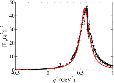
Figure 2: Fit to $|F_{\pi}(q^{2})|^{2}$ data using Eq. (8). The data are from Refs. PionFF_data_TL ; PionFF_data_SL .

In addition, the covariant spectator quark model built from this function describes well the $\Delta\to\gamma^{\ast}N$ form factor in the spacelike region as shown in Fig. 3. Using the best fit of $F_{\pi}$ given by the parameters (9) we can calculate the pion cloud contribution $G_{M}^{\pi}(q^{2})$ through Eq. (6), and consequently the result for $G_{M}^{\ast}(q^{2},M_{\Delta})$. For the parameters $\lambda_{\pi}$ and $\Lambda_{\pi}^{2}$ we use the results of the previous works $\lambda_{\pi}=0.441$ and $\Lambda_{\pi}^{2}=1.53\,\mathrm{GeV}^{2}$, obtained from the comparison of the constituent quark model to the lattice QCD data and experimental data NDeltaD ; LatticeD ; Timelike .

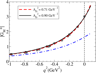
Figure 3: Results for $|G_{M}^{\ast}(q^{2})|$ for the covariant spectator quark model combined with the pion cloud contribution from Eq. (6). The data are from Refs. GM-Data . The dashed-dotted-line is the contribution from the core Timelike .

In Fig. 3 we present the result of our model for $|G_{M}^{\ast}(q^{2},W)|$ for the case $W=M_{\Delta}$. In that case the imaginary contribution (when $q^{2}>0$) is very small and the results can be compared with the spacelike data ($q^{2}<0$). In the figure the dashed-dotted-line indicate the result for $G_{M}^{B}(q^{2},M_{\Delta})$ discussed in a previous work Timelike .

In the same figure we show the sensitivity to the cutoff $\Lambda_{D}$ of the pion cloud model, by taking the cases $\Lambda_{D}^{2}=0.71\,\mathrm{GeV}^{2}$ and $\Lambda_{D}^{2}=0.90\,\mathrm{GeV}^{2}$. They are are consistent with the data, although the model with $\Lambda_{D}^{2}=0.71\,\mathrm{GeV}^{2}$ gives a slightly better description of the data. The two models are also numerically very similar to the results of Ref. Timelike for $W=M_{\Delta}$. For higher values of $W$ the results of the present model and the ones from Ref. Timelike will differ.

Although the model with $\Lambda_{D}^{2}=0.71\,\mathrm{GeV}^{2}$ gives a (slightly) better description of the spacelike data, for the generalization to the timelike region it is better to have a model with large effective cutoffs when compared with the scale of the $\rho$ meson pole (the $\rho$ mass $m_{\rho}$). This is important to separate the effects of the physical scales from the effective scales (adjusted cutoffs).

V Results

The results for $|G_{M}^{\ast}(q^{2})|$ from the covariant spectator quark model for the cases $W=1.232\,\mathrm{GeV}$, $W=1.6\,\mathrm{GeV}$, $W=1.8\,\mathrm{GeV}$, and $W=2.2\,\mathrm{GeV}$ are presented in Fig. 4. The thin lines represent the contribution from the bare quark core component of the model, and the thick line the sum of bare quark and pion cloud contributions.

In the figure the results for each value $W$ are restricted by the timelike kinematics through the condition $q^{2}\leq(W-M)^{2}$, since the nucleon and the resonance (with mass $W$) are treated both as being on their mass shells. Therefore the form factor covers an increasingly larger region on the $q^{2}$ axis, as $W$ increases. See Ref. Timelike for a complete discussion.

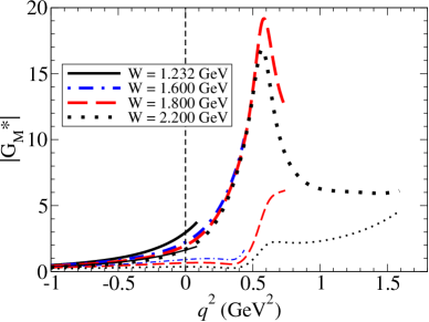
Figure 4: Results for $|G_{M}^{\ast}(Q^{2})|$ for $W=1.232\,\mathrm{GeV}$, $W=1.6\,\mathrm{GeV}$, $W=1.8\,\mathrm{GeV}$ and $W=2.2\,\mathrm{GeV}$. The thick lines indicate the final result. The thin lines indicate the contribution of the core.

The figure illustrates well the interplay between the pion cloud and the bare quark core components. The pion cloud component is dominating in the region near the $\rho$ peak. Away from that peak it is the bare quark contribution that dominates. The flatness of the $W=2.2\,\mathrm{GeV}$ curve for $q^{2}>1\,\mathrm{GeV}^{2}$ is the net result of the falloff of the pion cloud and the rise of the quark core terms. In addition, the figure shows that dependence on $W$ yields different magnitudes at the peak, and we recall that this dependence originates from the bare quark core contribution alone. This bare quark core contribution is mainly the consequence of the VMD parameterization of the quark current where there is an interplay between the effect of the $\rho$ pole and a term that behaves as a constant for intermediate values of $q^{2}$ (see Appendix A).

We will discuss now the results for the widths $\Gamma_{\gamma^{\ast}N}(q,W)$ of the $\Delta$ Dalitz decay, and for the $\Delta$ mass distribution $g_{\Delta}(W)$.

V.1 $\Delta$ Dalitz decay

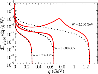
Figure 5: Results for $\frac{d\Gamma_{e^{+}e^{-}N}}{dq}(q,W)$ for three different values of energies $W$. The solid line is the result of our model. The dotted line is the result of the constant form factor model.

The width associated with the $\Delta$ decay into $\gamma^{\ast}N$ can be determined from the $\Delta\to\gamma^{\ast}N$ form factors for the $\Delta$ mass $W$. Assuming the dominance of the magnetic dipole form factors over the other two transition form factors, we can write Timelike ; Frohlich10 ; Krivoruchenko01

$$\begin{split}\Gamma_{\gamma^{\ast}N}(q,W)=&\frac{\alpha}{16}\frac{(W+M)^{2}}{M^{2}W^{3}}\\ &\times\sqrt{y_{+}y_{-}}y_{-}|G_{M}^{\ast}(q^{2},W)|,\end{split}$$ (10)

where $q=\sqrt{q^{2}}$, $\alpha\simeq 1/137$ is the fine-structure constant and $y_{\pm}=(W\pm M)^{2}-q^{2}$.

At the photon point ($q^{2}=0$), in particular, we obtain the $\Gamma_{\gamma N}$ in the limit $q^{2}=0$ from Eq. (10) Frohlich10 ; Wolf90 ; Krivoruchenko02

$$\Gamma_{\gamma N}(W)=\Gamma_{\gamma^{\ast}N}(0,W).$$ (11)

We can also calculate the derivative of the Dalitz decay width $\Gamma_{e^{+}e^{-}N}(q,W)$ from the function $\Gamma_{\gamma^{\ast}N}(q,W)$ using the relation Frohlich10 ; Wolf90 ; Krivoruchenko02 ; Krivoruchenko01

$$\begin{split}\Gamma^{\prime}_{e^{+}e^{-}N}(q,W)&\equiv\frac{\mathrm{d}\Gamma_{e^{+}e^{-}N}}{\mathrm{d}q}(q,W)\\ &=\frac{2\alpha}{3\pi q}\Gamma_{\gamma^{\ast}N}(q,W).\end{split}$$ (12)

The Dalitz decay width $\Gamma_{e^{+}e^{-}N}(q,W)$ is given by

$$\Gamma_{e^{+}e^{-}N}(W)=\int_{2m_{e}}^{W-M}\Gamma^{\prime}_{e^{+}e^{-}N}(q,W)\,\mathrm{d}q,$$ (13)

where $m_{e}$ is the electron mass. Note that the integration holds for the interval $4m_{e}^{2}\leq q^{2}\leq(W-M)^{2}$, where the lower limit is the minimum value necessary to produce an $\mathrm{e}^{+}\mathrm{e}^{-}$ pair, and $(W-M)^{2}$ is the maximum value available in the $\Delta\to\gamma^{\ast}N$ decay for a given $W$ value.

The results for $\frac{\mathrm{d}\Gamma_{e^{+}e^{-}N}}{\mathrm{d}q}(q,W)$ for several mass values $W$ (1.232, 1.6 and 2.2 GeV) are presented in Fig. 5. These results are also compared to the calculation given by the constant form factor model, from which they deviate considerably.

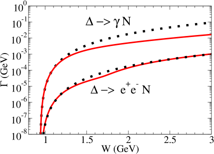
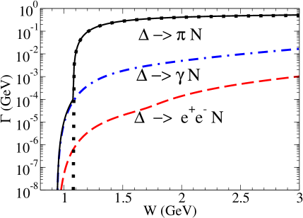
Figure 6: Results for the partial widths as function of $W$. At left: partial widths (solid line) for $\Delta\to\gamma N$ and $\Delta\to e^{+}e^{-}N$, compared with the constant form factor model (dotted line). At right: the partial widths are compared with the $\Delta\to\pi N$ width (dotted line) and with the sum of all widths (thin solid line).

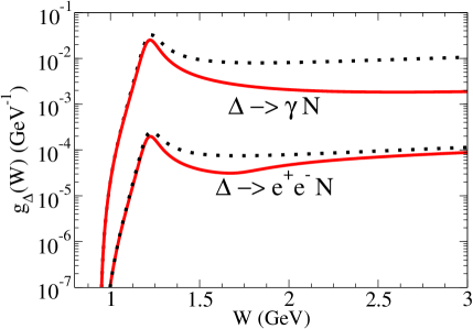
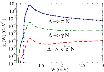
Figure 7: Results for $g_{\Delta}(W)$ and the partial contributions $g_{\Delta\to\pi N}(W)$, $g_{\Delta\to\gamma N}(W)$ and $g_{\Delta\to e^{+}e^{-}N}(W)$. At left: $g_{\Delta\to\gamma N}(W)$ and $g_{\Delta\to e^{+}e^{-}N}(W)$ in comparison with constant form factor model (dotted line). At right: all contributions compared with the total $g_{\Delta}(W)$ (thin solid line).

Also, the $\Delta$ decay width can be decomposed at tree level into three independent channels

$$\Gamma_{\rm tot}(W)=\Gamma_{\pi N}(W)+\Gamma_{\gamma N}(W)+\Gamma_{e^{+}e^{-}N}(W),$$ (14)

given by the decays $\Delta\to\pi N$, $\Delta\to\gamma N$ and $\Delta\to e^{+}e^{-}N$. The two last terms are described respectively by Eqs. (11) and (13). The $\Gamma_{\pi N}$ term can be parameterized as in Manley92 ; Buss11

$$\Gamma_{\pi N}(W)=\frac{M_{\Delta}}{W}\left(\frac{q_{\pi}(W)}{q_{\pi}(M_{\Delta})}\right)^{3}\frac{\kappa^{2}+q_{\pi}^{2}(M_{\Delta})}{\kappa^{2}+q_{\pi}^{2}(W)}\Gamma_{\pi N}^{0},$$ (15)

where $\Gamma_{\pi N}^{0}$ is the $\Delta\to\pi N$ partial width for the physical $\Delta$, $q_{\pi}(W)$ is the pion momentum for a $\Delta$ decay with mass $W$, and $\kappa$ a cutoff parameter. Following Refs. Weil12 ; Weil14 we took $\kappa=0.197$ GeV. The present parameterization differs from other forms used in the literature Frohlich10 ; Wolf90 and from our previous work Timelike .

The results for the partial widths as functions of the mass $W$ are presented in Fig. 6. On the left panel we compare $\Gamma_{\gamma N}$ and $\Gamma_{e^{+}e^{-}N}$ with the result of the constant form factor model. On the right panel we present the total width $\Gamma_{\rm tot}(W)$ as the sum of the three partial widths.

V.2 $\Delta$ mass distribution

To study the impact of the $\Delta$ resonance propagation in nuclear reactions like the $NN$ reaction, it is necessary to know the $\Delta$ mass distribution function $g_{\Delta}(W)$. As discussed before, $W$ is an arbitrary resonance mass that may differ from the resonance pole mass ($M_{\Delta}$). The usual ansatz for $g_{\Delta}$ is the relativistic Breit-Wigner distribution-Timelike ; Frohlich10

$$g_{\Delta}(W)=A\frac{W^{2}\Gamma_{\rm tot}(W)}{(W^{2}-M_{\Delta}^{2})^{2}+W^{2}\left[\Gamma_{\rm tot}(W)\right]^{2}},$$ (16)

where $A$ is a normalization constant determined by $\int g_{\Delta}(W)\mathrm{d}W=1$ and the total width $\Gamma_{\rm tot}(W)$ (15).

The results for $g_{\Delta}(W)$ and the partial contributions

Figure 8: Transport-model calculations of dilepton mass spectra $\mathrm{d}\sigma/\mathrm{d}m_{ee}$ from proton-proton collisions $(pp\to e^{+}e^{-}X)$ at three different beam energies, with and without a $\Delta\to\gamma^{\ast}N$ form factor, compared to experimental data measured with the HADES detector Agakishiev09 ; Agakishiev12 ; HADES12 .

$$g_{\Delta\to\gamma N}(W)=\frac{\Gamma_{\gamma N}(W)}{\Gamma_{\rm tot}(W)}g_{\Delta}(W),$$ (17)

$$g_{\Delta\to e^{+}e^{-}N}(W)=\frac{\Gamma_{e^{+}e^{-}N}(W)}{\Gamma_{\rm tot}(W)}g_{\Delta}(W),$$ (18)

$$g_{\Delta\to\pi N}(W)=\frac{\Gamma_{\pi N}(W)}{\Gamma_{\rm tot}(W)}g_{\Delta}(W),$$ (19)

are presented in Fig. 7. The results are also compared with the constant form factor model.

V.3 Dilepton production from $NN$ collisions

The $\Delta\to\gamma^{\ast}N$ magnetic dipole form factor in the timelike region is known to have a significant influence on dilepton spectra. Therefore we show in Fig. 8 a transport-model calculation of the inclusive dielectron production cross section $\mathrm{d}\sigma/\mathrm{d}m_{\text{ee}}$ for proton-proton collisions $(\text{pp}\to\mathrm{e}^{+}\mathrm{e}^{-}X)$, where $m_{\text{ee}}=q$. These results have been obtained with the GiBUU model Buss11 ; Weil12 for three different proton beam energies and are compared to experimental data measured with the HADES detector Agakishiev09 ; Agakishiev12 ; HADES12 . Except for the contribution of the $\Delta$ Dalitz decay, the calculations are identical to those presented in an earlier publication Weil14 . The $\Delta$ Dalitz decay is shown in two variants, once with a constant form factor fixed at the photon point (i.e., in ’QED’ approximation) and once using the form-factor model described in the preceding sections.

At the lowest beam energy of 1.25 GeV, the produced $\Delta$ baryons are close to the pole mass and therefore the results with and without the form factor are very similar. At higher beam energies, however, the model for the $\Delta\to\gamma^{\ast}N$ form factor has a much larger impact, because higher values of $W$ are reached, where the form factor deviates strongly from the photon point value. In Fig. 9 we illustrate the influence of $W$ by showing the $W$ distribution of produced $\Delta^{+,0}$ baryons in the GiBUU simulations. We note that several different processes contribute to the inclusive $\Delta^{+,0}$ production, such as $NN\rightarrow N\Delta,\;\Delta\Delta,\;\Delta N^{*}$ etc., each of which will produce a different $W$ distribution due to different kinematics and phase space. Furthermore it should be remarked that the tails of this distribution, just as the $\Delta$ spectral function in Eq. (16), depend significantly on the specific parameterization of the hadronic width for $\Delta\rightarrow\pi N$. However, for electromagnetic observables as shown in Fig. 8, the dependence on the hadronic width is very weak, since in Eq. (18) the total width cancels out in the numerator and only stays in the denominator.

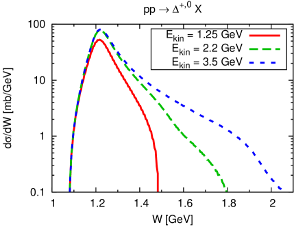
Figure 9: Mass distribution of produced $\Delta^{+,0}$ baryons in GiBUU simulations, for pp collisions at three different beam energies.

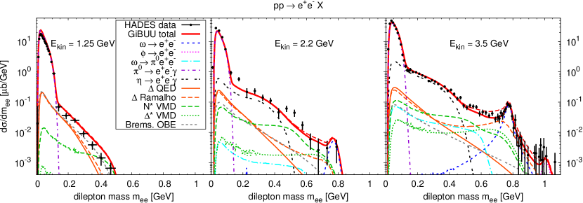
Figure 10: Modified calculations of dilepton mass spectra $\mathrm{d}\sigma/\mathrm{d}m_{\text{ee}}$ from proton-proton collisions $(\text{pp}\to\text{e}^{+}\text{e}^{-}X)$, using reduced $R\rightarrow\rho N$ branching ratios for two resonances (see text).

Coming back to Fig. 8, it should be noted that the choice of the form factor has little influence on the overall agreement of the total dilepton spectrum with the experimental data at the two lowest beam energies, because the influence of the form factor is weak or the $\Delta$ contribution is small compared to other channels. At the highest beam energy of 3.5 GeV, however, the choice of the form factor does have an impact on the total spectrum for masses above 600 MeV. While the constant-form-factor result combined with the other channels from GiBUU shows a good agreement with the data, using the $q^{2}$ dependent form factor results in a slight overestimation of the data, which is most severe for masses of around 700 MeV. However, we note that the $\Delta$ contribution by itself does not overshoot the data. Only in combination with the other channels (in particular the heavier baryons, such as $N^{*}$ and $\Delta^{*}$) the overestimation is seen.

There could be various reasons for this enhancement over the data, but we want to mention here only the two most likely ones. One could lie in the form factor itself, more precisely in the omission of an $W$ dependence of the overall weight $\lambda_{\pi}$ for the pion cloud. This parameter for the weight of the pion cloud should probably depend on $W$. If the two diagrams (a) and (b) of the pion cloud contribution would decrease simultaneously with $W$, as we can expect from the drop of the $m_{\pi}/W$ ratio, this could potentially cure the observed overestimation.

On the other hand, the reason for the disagreement could also be found in the other channels that are part of the transport calculation. In particular the contributions of the higher baryonic resonances ($N^{*}$ and $\Delta^{*}$) are subject to some uncertainties. These resonance contributions were recently investigated via exclusive pion production at 3.5 GeV with the HADES detector Agakishiev14 , which showed that the GiBUU model does a rather good job in describing the resonance cocktail for the exclusive channels (with some minor deviations). However, there are also significant non-exclusive channels for pion and dilepton production at this energy. Moreover, the form factors of the higher resonances are a matter of debate (they are treated in a strict-VMD assumption in the calculation).

It was remarked in Agakishiev14 that some of the branching ratios for $R\rightarrow\rho N$, which directly influence the dilepton yield via the VMD assumption, might be overestimated in GiBUU, in particular for the $N^{*}(1720)$ and the $\Delta^{*}(1905)$. Both have a very large $\rho N$ branching ratio of 87% in GiBUU Weil12 (as adopted from Manley92 ) and also in the current PDG database these branching ratios are listed with rather large values PDG14 , which are essentially compatible with the GiBUU values. However, some recent partial-wave analyses BonnGatchina ; KSU claim much smaller values for these branching ratios, showing some tension with the PDG and GiBUU values. We show in Fig. 10 the effect of using smaller values for these branching ratios on the dilepton spectra, adopting the upper limits from the Bonn-Gatchina analysis BonnGatchina (as given in Agakishiev14 ), namely 10% for $N^{*}(1720)\rightarrow\rho N$ and 42% for $\Delta^{*}(1905)\rightarrow\rho N$. We note that the values in KSU are even smaller. As seen in Fig. 10, this change indeed reduces the contributions from the $N^{*}$ and $\Delta^{*}$ resonances by a fair amount, in particular in the high-mass region ($m_{ee}>600$ MeV). This improves the agreement with the highest data points at 2.2 GeV, and it also mitigates the overshooting over the data at 3.5 GeV when the $\Delta\to\gamma^{\ast}N$ form factor is used, but it does not fully cure it.

Thus it is quite likely that the remaining excess is caused by the negligence of the $W$ dependence in the pion cloud contribution of the form factor. A more detailed investigation of the $W$ dependence of the pion cloud is planned in a further study that will analyze all these aspects.

VI Summary and conclusions

In this work we present a new covariant model for the $\Delta\to\gamma^{\ast}N$ transition in the timelike region. The model is based on the combination of valence quark and meson cloud degrees of freedom. The bare quark contribution was calibrated previously to lattice QCD data. One of the pion cloud components is fitted to the pion electromagnetic form factor $F_{\pi}$ (with the fit being almost insensitive to the spacelike data and strongly dependent on the timelike data) and the other, associated with intermediate octet/decuplet baryon states, parameterized by an effective cutoff $\Lambda_{D}$.

Our model induces a strong effect on the $\Delta\to\gamma^{\ast}N$ magnetic dipole form factor in the region around the $\rho-$meson pole (where the magnitude is about four times larger than at $q^{2}=0$). This effect was missing in the frequently used Iachello model. The pion cloud effects dominate in the region $q^{2}\leq 1.5\,\mathrm{GeV}^{2}$. For larger $q^{2}$ the effects of the valence quark became dominant, and the $q^{2}$-dependence is smoother. At low energies, the new form factor has little influence on the overall agreement of the total dilepton spectrum in $NN$ collisions with the experimental data, and no large difference between our new model and the VMD model is seen. However at the highest beam energy of 3.5 GeV, the choice of the form factor does affect the total spectrum for masses above 600 MeV.

Measurements of independent channels, for instance exclusive pion induced $\Delta$ production data, can help to better constrain the pion cloud contribution. The methods presented in this work can in principle be extended to higher mass resonances as $N^{\ast}(1440)$, $N^{\ast}(1520)$, $N^{\ast}(1535)$, $N^{\ast}(1710)$ and $\Delta^{\ast}(1600)$, for which there are already predictions of the covariant spectator quark model N1520 ; Resonances in the spacelike region. The calculation of the $N^{\ast}(1520)$ form factors in the timelike region N1520TL , extending the results from Ref. N1520 is already under way.

Appendix A Quark form factors

We use a parameterization of the quark isovector form factors motivated by VMD Nucleon ; Lattice ; LatticeD

$$\begin{split}&f_{1-}(q^{2})=\lambda_{q}+(1-\lambda_{q})\frac{m_{\rho}^{2}}{m_{\rho}^{2}-q^{2}}-c_{-}\frac{M_{h}^{2}q^{2}}{(M_{h}^{2}-q^{2})^{2}}\\ &f_{2-}(q^{2})=\kappa_{-}\left\{d_{-}\frac{m_{\rho}^{2}}{m_{\rho}^{2}-q^{2}}+(1-d_{-})\frac{M_{h}^{2}}{M_{h}^{2}-q^{2}}\right\},\end{split}$$ (20)

where $m_{\rho}=775$ MeV is the $\rho$-meson mass, $M_{h}$ is the mass of an effective heavy vector meson, $\kappa_{-}$ is the quark isovector anomalous magnetic moment, $c_{-}$, $d_{-}$ are mixture coefficients, and $\lambda_{q}$ is a parameter related with the quark density number in the deep inelastic limit Nucleon . The term in $M_{h}$, where $M_{h}=2M$, simulates the effects of the heavier mesons (short range physics) Nucleon , and behaves as a constant for values of $q^{2}$ much smaller than $4M^{2}$. The width associated with the pole $q^{2}=M_{h}^{2}$ is discussed in the Appendix B.

The $\rho$ pole appears when one assumes a stable $\rho$ with zero decay width $\Gamma_{\rho}=0$. For the extension of the quark form factors to the timelike regime we consider therefore the replacement

$$\frac{m_{\rho}^{2}}{m_{\rho}^{2}-q^{2}}\to\frac{m_{\rho}^{2}}{m_{\rho}^{2}-q^{2}-\mathrm{i}m_{\rho}\Gamma_{\rho}(q^{2})}.$$ (21)

On the r.h.s. we introduce $\Gamma_{\rho}$ the $\rho$ decay width as a function of $q^{2}$.

The function $\Gamma_{\rho}(q^{2})$ represents the $\rho\to 2\pi$ decay width for a virtual $\rho$ with momentum $q^{2}$ Gounaris68 ; Connell97

$$\Gamma_{\rho}(q^{2})=\Gamma_{\rho}^{0}\frac{m_{\rho}^{2}}{q^{2}}\left(\frac{q^{2}-4m_{\pi}^{2}}{m_{\rho}^{2}-4m_{\pi}^{2}}\right)^{\frac{3}{2}}\theta(q^{2}-4m_{\pi}^{2}),$$ (22)

where $\Gamma_{\rho}^{0}=0.149$ GeV.

Appendix B Regularization of high momentum poles

For a given $W$ the squared momentum $q^{2}$ is limited by the kinematic condition $q^{2}\leq(W-M)^{2}$. Then, if one has a singularity at $q^{2}=\Lambda^{2}$, that singularity will appear for values of $W$ such that $\Lambda^{2}\leq(W-M)^{2}$, or $W\geq M+\Lambda$.

To avoid a singularity at $q^{2}=\Lambda^{2}$, where $\Lambda^{2}$ is any of the cutoffs introduced in our pion cloud parameterizations, and quark current (pole $M_{h}$) we implemented a simple procedure. We start with

$$\frac{\Lambda^{2}}{\Lambda^{2}-q^{2}}\to\frac{\Lambda^{2}}{\Lambda^{2}-q^{2}-\mathrm{i}\Lambda\Gamma_{X}(q^{2})},$$ (23)

where

$$\Gamma_{X}(q^{2})=4\Gamma_{X}^{0}\left(\frac{q^{2}}{q^{2}+\Lambda^{2}}\right)^{2}\theta(q^{2}),$$ (24)

In the last equation $\Gamma_{X}^{0}$ is a constant given by $\Gamma_{X}^{0}=4\Gamma_{\rho}^{0}\simeq 0.6$ GeV.

In Eq. (24) the function $\Gamma_{X}(q^{2})$ is defined such that $\Gamma_{X}(q^{2})=0$ when $q^{2}<0$. Therefore the results in the spacelike region are kept unchanged. For $q^{2}=\Lambda^{2}$ we obtain $\Gamma_{X}=\Gamma_{X}^{0}$, and for very large $q^{2}$ it follows $\Gamma_{X}\simeq 4\Gamma_{X}^{0}$. Finally the value of $\Gamma_{X}^{0}$ was chosen to avoid very narrow peaks around $\Lambda^{2}$.

While the width $\Gamma_{\rho}(q^{2})$ associated with the $\rho$-meson pole in the quark current is nonzero only when $q^{2}>4m_{\pi}^{2}$, one has for $\Gamma_{X}(q^{2})$ nonzero values also in the interval $4m_{\pi}^{2}>q^{2}>0$. However, the function $\Gamma_{X}(q^{2})$ changes smoothly in that interval and its values are negligible.

This procedure was used in Ref. Timelike ; Weil12 for the calculation of the $\Delta\to\gamma^{\ast}N$ form factors in the timelike regime. In the present case the emerging singularities for $W>M+\Lambda_{D}\simeq 1.84\,\mathrm{GeV}$ are avoided, and for $W<1.84\,\mathrm{GeV}$, the results are almost identical to the ones without regularization. The suggested procedure avoids the singularities at high momentum and at the same time preserves the results for low momentum. In the cases considered the high $q^{2}$ contributions are suppressed and the details of regularization procedure are not important.

References

- (1) I. G. Aznauryan, A. Bashir, V. Braun, S. J. Brodsky, V. D. Burkert, L. Chang, C. Chen and B. El-Bennich et al., Int. J. Mod. Phys. E 22, 1330015 (2013) [arXiv:1212.4891 [nucl-th]].
- (2) W. J. Briscoe, M. Döring, H. Haberzettl, D. M. Manley, M. Naruki, I. I. Strakovsky and E. S. Swanson, Eur. Phys. J. A 51, 129 (2015) [arXiv:1503.07763 [hep-ph]].
- (3) G. Agakishiev et al., Eur. Phys. J. A 50, 82 (2014) [arXiv:1403.3054 [nucl-ex]].
- (4) G. Ramalho and M. T. Peña, Phys. Rev. D 85, 113014 (2012) [arXiv:1205.2575 [hep-ph]].
- (5) F. Dohrmann et al., Eur. Phys. J. A 45, 401 (2010) [arXiv:0909.5373 [nucl-ex]].
- (6) G. Ramalho, M. T. Peña and F. Gross, Eur. Phys. J. A 36, 329 (2008) [arXiv:0803.3034 [hep-ph]].
- (7) G. Ramalho, M. T. Peña and F. Gross, Phys. Rev. D 78, 114017 (2008) [arXiv:0810.4126 [hep-ph]].
- (8) G. Ramalho and M. T. Peña, Phys. Rev. D 80, 013008 (2009) [arXiv:0901.4310 [hep-ph]].
- (9) G. Ramalho and K. Tsushima, Phys. Rev. D 87, 093011 (2013) [arXiv:1302.6889 [hep-ph]].
- (10) G. Ramalho and K. Tsushima, Phys. Rev. D 88, 053002 (2013) [arXiv:1307.6840 [hep-ph]].
- (11) S. S. Kamalov, S. N. Yang, D. Drechsel, O. Hanstein and L. Tiator, Phys. Rev. C 64, 032201 (2001) [arXiv:nucl-th/0006068]; T. Sato and T. S. H. Lee, Phys. Rev. C 63, 055201 (2001) [arXiv:nucl-th/0010025].
- (12) V. M. Braun, A. Lenz, G. Peters and A. V. Radyushkin, Phys. Rev. D 73, 034020 (2006) [hep-ph/0510237].
- (13) C. Alexandrou, G. Koutsou, J. W. Negele, Y. Proestos and A. Tsapalis, Phys. Rev. D 83, 014501 (2011) [arXiv:1011.3233 [hep-lat]].
- (14) G. Eichmann and D. Nicmorus, Phys. Rev. D 85, 093004 (2012) [arXiv:1112.2232 [hep-ph]].
- (15) J. Segovia, C. Chen, I. C. Cloët, C. D. Roberts, S. M. Schmidt and S. Wan, Few Body Syst. 55, 1 (2014) [arXiv:1308.5225 [nucl-th]].
- (16) M. Schafer, H. C. Donges, A. Engel and U. Mosel, Nucl. Phys. A 575, 429 (1994) [nucl-th/9401006].
- (17) F. de Jong and U. Mosel, Phys. Lett. B 392, 273 (1997) [nucl-th/9611051].
- (18) M. I. Krivoruchenko, B. V. Martemyanov, A. Faessler and C. Fuchs, Annals Phys. 296, 299 (2002) [arXiv:nucl-th/0110066].
- (19) A. Faessler, C. Fuchs, M. I. Krivoruchenko and B. V. Martemyanov, J. Phys. G 29, 603 (2003) [nucl-th/0010056].
- (20) M. Zetenyi and G. Wolf, Phys. Rev. C 67, 044002 (2003) [arXiv:nucl-th/0103062].
- (21) F. Iachello, A. D. Jackson and A. Lande, Phys. Lett. B 43, 191 (1973).
- (22) F. Iachello and Q. Wan, Phys. Rev. C 69, 055204 (2004); R. Bijker and F. Iachello, Phys. Rev. C 69, 068201 (2004) [arXiv:nucl-th/0405028].
- (23) G. Ramalho and M. T. Peña, J. Phys. G 36, 115011 (2009) [arXiv:0812.0187 [hep-ph]].
- (24) B. Julia-Diaz, H. Kamano, T. S. Lee, A. Matsuyama, T. Sato and N. Suzuki, Phys. Rev. C 80, 025207 (2009).
- (25) F. Gross, G. Ramalho and M. T. Peña, Phys. Rev. C 77, 015202 (2008) [nucl-th/0606029].
- (26) F. Gross, G. Ramalho and M. T. Peña, Phys. Rev. D 85, 093005 (2012) [arXiv:1201.6336 [hep-ph]].
- (27) G. Ramalho, K. Tsushima and F. Gross, Phys. Rev. D 80, 033004 (2009) [arXiv:0907.1060 [hep-ph]].
- (28) C. E. Carlson and J. L. Poor, Phys. Rev. D 38, 2758 (1988); C. E. Carlson, Few Body Syst. Suppl. 11, 10 (1999) [arXiv:hep-ph/9809595].
- (29) A. D. Bukin et al., Phys. Lett. B 73, 226 (1978); A. Quenzer et al., Phys. Lett. B 76, 512 (1978); L. M. Barkov et al., Nucl. Phys. B 256, 365 (1985); R. R. Akhmetshin et al. [CMD-2 Collaboration], Phys. Lett. B 527, 161 (2002) [hep-ex/0112031]; R. R. Akhmetshin et al. [CMD-2 Collaboration], Phys. Lett. B 648, 28 (2007) [hep-ex/0610021].
- (30) S. R. Amendolia et al. [NA7 Collaboration], Nucl. Phys. B 277, 168 (1986); C. N. Brown et al., Phys. Rev. D 8, 92 (1973); C. J. Bebek et al., Phys. Rev. D 9, 1229 (1974); C. J. Bebek, C. N. Brown, M. Herzlinger, S. D. Holmes, C. A. Lichtenstein, F. M. Pipkin, S. Raither and L. K. Sisterson, Phys. Rev. D 13, 25 (1976); C. J. Bebek et al., Phys. Rev. D 17, 1693 (1978); G. M. Huber et al. [Jefferson Lab Collaboration], Phys. Rev. C 78, 045203 (2008) [arXiv:0809.3052 [nucl-ex]].
- (31) W. Bartel, B. Dudelzak, H. Krehbiel, J. McElroy, U. Meyer-Berkhout, W. Schmidt, V. Walther and G. Weber, Phys. Lett. B 28, 148 (1968); S. Stein et al., Phys. Rev. D 12, 1884 (1975); K. Nakamura et al. [Particle Data Group Collaboration], J. Phys. G 37, 075021 (2010).
- (32) H. B. O’Connell, B. C. Pearce, A. W. Thomas and A. G. Williams, Prog. Part. Nucl. Phys. 39, 201 (1997) [hep-ph/9501251].
- (33) H. C. Donges, M. Schafer and U. Mosel, Phys. Rev. C 51, 950 (1995) [nucl-th/9407012].
- (34) J. Weil, H. van Hees, and U. Mosel, Eur. Phys. J. A 48, 111 (2012) [Erratum-ibid. A 48, 150 (2012)] [arXiv:1203.3557 [nucl-th]].
- (35) J. Weil, S. Endres, H. van Hees, M. Bleicher and U. Mosel, arXiv:1410.4206 [nucl-th].
- (36) D. M. Manley and E. M. Saleski, Phys. Rev. D 45 4002 (1992).
- (37) G. Wolf, G. Batko, W. Cassing, U. Mosel, K. Niita and M. Schaefer, Nucl. Phys. A 517, 615 (1990).
- (38) M. I. Krivoruchenko and A. Faessler, Phys. Rev. D 65, 017502 (2001) [arXiv:nucl-th/0104045].
- (39) O. Buss et al., Phys. Rept. 512, 1 (2012) [arXiv:1106.1344 [hep-ph]].
- (40) G. Agakishiev et al. [HADES Collaboration], Phys. Lett. B 690, 118 (2010) [arXiv:0910.5875 [nucl-ex]].
- (41) G. Agakishiev et al. [HADES Collaboration], Phys. Rev. C 85, 054005 (2012) [arXiv:1203.2549 [nucl-ex]].
- (42) G. Agakishiev et al. [HADES Collaboration], Eur. Phys. J. A 48, 64 (2012) [arXiv:1112.3607 [nucl-ex]].
- (43) G. Agakishiev et al., Eur. Phys. J. A 50, 82 (2014). [arXiv:1403.3054 [nucl-ex]].
- (44) K. A. Olive et al. [Particle Data Group Collaboration], Chin. Phys. C 38 (2014) 090001.
- (45) A. V. Anisovich, R. Beck, E. Klempt, V. A. Nikonov, A. V. Sarantsev and U. Thoma, Eur. Phys. J. A 48 (2012) 15 [arXiv:1112.4937 [hep-ph]].
- (46) M. Shrestha and D. M. Manley, Phys. Rev. C 86 (2012) 055203 [arXiv:1208.2710 [hep-ph]].
- (47) G. Ramalho and M. T. Peña, Phys. Rev. D 89, 094016 (2014) [arXiv:1309.0730 [hep-ph]].
- (48) G. Ramalho and K. Tsushima, Phys. Rev. D 81, 074020 (2010) [arXiv:1002.3386 [hep-ph]]; G. Ramalho and K. Tsushima, Phys. Rev. D 82, 073007 (2010) [arXiv:1008.3822 [hep-ph]]; G. Ramalho and M. T. Peña, Phys. Rev. D 84, 033007 (2011) [arXiv:1105.2223 [hep-ph]]; G. Ramalho and K. Tsushima, Phys. Rev. D 89, 073010 (2014) [arXiv:1402.3234 [hep-ph]].
- (49) G. Ramalho and M. T. Peña, work in progress.
- (50) G. J. Gounaris and J. J. Sakurai, Phys. Rev. Lett. 21, 244 (1968).