Effective field theory in the harmonic oscillator basis

Abstract

We develop interactions from chiral effective field theory (EFT) that are tailored to the harmonic oscillator basis. As a consequence, ultraviolet convergence with respect to the model space is implemented by construction and infrared convergence can be achieved by enlarging the model space for the kinetic energy. In oscillator EFT, matrix elements of EFTs formulated for continuous momenta are evaluated at the discrete momenta that stem from the diagonalization of the kinetic energy in the finite oscillator space. By fitting to realistic phase shifts and deuteron data we construct an effective interaction from chiral EFT at next-to-leading order. Many-body coupled-cluster calculations of nuclei up to ¹³²Sn converge fast for the ground-state energies and radii in feasible model spaces.

I Introduction

The harmonic oscillator basis is advantageous in nuclear-structure theory because it retains all symmetries of the atomic nucleus and provides an approximate mean-field related to the nuclear shell model. However, interactions from chiral effective field theory (EFT) Epelbaum et al. (2009); Machleidt and Entem (2011) are typically formulated in momentum space, while the oscillator basis treats momenta and coordinates on an equal footing, thereby mixing long- and short-ranged physics. This incommensurability between the two bases is not only of academic concern but also makes oscillator-based ab initio calculations numerically expensive. Indeed, the oscillator basis must be large enough to accommodate the nucleus in position space as well as to contain the high-momentum contributions of the employed interaction. Furthermore, one needs to perform computations at different values of the oscillator spacing $\hbar\omega$ to gauge model-space independence of the computed results Maris et al. (2009); Hagen et al. (2010); Jurgenson et al. (2013); Roth et al. (2014). Several methods have been proposed to alleviate these problems. Renormalization group transformations, for instance, are routinely used to “soften” interactions Bogner et al. (2003, 2007); Roth et al. (2014), and many insights have been gained through these transformations Jurgenson et al. (2009). However, such transformations of the Hamiltonian and observables Lisetskiy et al. (2009); Schuster et al. (2014) add one layer of complexity to computations of nuclei.

One can contrast the effort of computations in the oscillator basis to, for instance, computations in nuclear lattice EFT Lee (2009). Here, the effective interaction is tailored to the lattice spacing and, thus, to the ultraviolet (UV) cutoff, and well-known extrapolation formulas Lüscher (1986) can be used to estimate corrections due to finite lattice sizes. The lattice spacing is fixed once, reducing the computational expenses. This motivates us to seek a similarly efficient approach for the oscillator basis, i.e., to formulate an EFT for nuclear interactions directly in the oscillator basis.

In recent years, realistic ab initio nuclear computations pushed the frontier from light $p$-shell nuclei Navrátil et al. (2009); Barrett et al. (2013) to the medium-mass regime Hagen et al. (2012); Holt et al. (2012); Wienholtz et al. (2013); Somà et al. (2014); Lähde et al. (2014); Hagen et al. (2014); Hergert et al. (2014); Hagen et al. (2016). At present, the precision of computational methods considerably exceeds the accuracy of available interactions Binder et al. (2014), and this is the main limitation in pushing the frontier of ab initio computations to heavy nuclei. To address this situation, several efforts, ranging from new optimization protocols for chiral interactions Ekström et al. (2013, 2015); Carlsson et al. (2016) to the inclusion of higher orders Entem et al. (2015); Epelbaum et al. (2015) to the development of interactions with novel regulators Gezerlis et al. (2014) are under way. To facilitate the computation of heavy nuclei we propose to tailor interactions from chiral EFT to the oscillator basis.

There exist several proposals to formulate EFTs in the oscillator basis. Haxton and coworkers proposed the oscillator based effective theory (HOBET) Haxton and Song (2000); Haxton and Luu (2002); Haxton (2007, 2008). They focused on decoupling low- and high-energy modes in the oscillator basis via the Bloch-Horowitz formalism, and on the resummation of the kinetic energy to improve the asymptotics of bound-state wave functions in configuration space. The HOBET interaction is based on a contact-gradient expansion, and the matrix elements are computed in the oscillator basis. The resulting interaction exhibits a weak energy dependence. The Arizona group Stetcu et al. (2007, 2010); Rotureau et al. (2012) posed and studied questions related to the UV and infrared (IR) cutoffs imposed by the oscillator basis, and developed a pion-less EFT in the oscillator basis. This EFT was also applied to harmonically trapped atoms Rotureau et al. (2010). In this approach, the interaction matrix elements are also based on a contact-gradient expansion and computed in the oscillator basis. Running coupling constants depend on the UV cutoff of the employed oscillator basis. In a sequence of other papers, Tölle et al. studied harmonically trapped few-boson systems in an effective field theory based on contact interactions with running coupling constants Tölle et al. (2011, 2013).

Our oscillator EFT differs from these approaches. For the interaction we choose an oscillator space with a fixed oscillator frequency $\omega$ and a fixed maximum energy $(N_{\rm max}+\nicefrac{{3}}{{2}})\,\hbar\omega$. The matrix elements of the interaction are taken from an EFT formulated in momentum space and evaluated at the discrete momentum eigenvalues of the kinetic energy in this fixed oscillator space. This reformulation, or projection, of a momentum-space EFT onto a finite oscillator model space requires us to re-fit the low-energy coefficients (LECs) of interactions at a given order of the EFT. We determine these by an optimization to scattering phase shifts (computed in the finite oscillator basis via the $J$-matrix approach Heller and Yamani (1974); Shirokov et al. (2004)) and from deuteron properties. The power counting of the oscillator EFT is based on that of the underlying momentum-space EFT. The finite oscillator space introduces IR and UV cutoffs Stetcu et al. (2007); Coon et al. (2012); Furnstahl et al. (2012); More et al. (2013); Furnstahl et al. (2014); König et al. (2014); Furnstahl et al. (2015a); Wendt et al. (2015), and these are thus fixed for the interaction.

In practical many-body calculations we will keep the oscillator frequency and the interaction fixed at $\hbar\omega$ and $N_{\rm max}$, but employ the kinetic energy in larger model spaces. This increase of the model space increases (decreases) its UV (IR) cutoff but does not change any interaction matrix elements and thus leaves the IR and UV cutoff of the interaction unchanged. As UV convergence of the many-body calculations depends on the matrix elements of an interaction König et al. (2014), oscillator EFT guarantees this UV convergence by construction because no new potential matrix elements enter beyond $N_{\rm max}$. We stress that our notion of UV convergence relates to the convergence of the many-body calculations and should not be confused with the expectation that observables are independent of the regulator or cutoff. Infrared convergence builds up the exponential tail of bound-state wave functions in position space, as the effective IR cutoff of a finite nucleus is set by its radius. Thus, the increase of the model space for the kinetic energy achieves IR convergence. Regarding IR convergence, oscillator EFT is similar to the HOBET of Ref. Haxton (2007). In practice, IR-converged values for bound-state energies and radii can be obtained applying “Lüscher-like” formulas for the oscillator basis Furnstahl et al. (2012).

We view oscillator EFT similar to lattice EFT Lee (2009). The latter constructs an interaction on a lattice in position space while the former builds an interaction on a discrete (but non-equidistant) mesh in momentum space. In both EFTs the UV cutoff of the interaction is fixed once and for all, and LECs are adjusted to scattering data and bound states. The increase in lattice sites achieves IR convergence in lattice EFT, while the increase of the number of oscillator shells achieves IR convergence in oscillator EFT.

As we will see, the resulting EFT interaction in the oscillator basis exhibits a fast convergence, similar to the phenomenological JISP interaction Shirokov et al. (2007). From a practical point of view, our approach to oscillator EFT allows us to employ all of the existing infrastructure developed for nuclear calculations.

The discrete basis employed in this paper is actually the basis set of a discrete variable representation (DVR) Harris et al. (1965); Dickinson and Certain (1968); Light et al. (1985); Baye and Heenen (1986); Littlejohn et al. (2002); Light and Carrington (2007); Bulgac and McNeil Forbes (2013) in momentum space. While coordinate-space DVRs are particularly useful and popular in combination with local potentials, the results of this paper suggest that DVRs are also useful in momentum-space-based EFTs, because they facilitate the evaluation of matrix elements.

This paper is organized as follows. In Section II we analyze the momentum-space structure of a finite oscillator basis. In Section III we validate our approach by reproducing an interaction from chiral EFT at next-to-leading order (NLO). In Section IV we construct a NLO interaction from realistic phase shifts and employ this interaction in many-body calculations, demonstrating that converged binding energies and radii can be obtained for nuclei in the mass-100 region in model spaces with $N_{\rm max}=$ 10 to 14 without any further renormalization. We finally present our summary in Section V.

II Theoretical considerations

In this Section we present the theoretical foundation of an EFT in the oscillator basis. We derive analytical expressions for the momentum eigenstates and eigenvalues in finite oscillator spaces and present useful formulas for interaction matrix elements.

II.1 Momentum states in finite oscillator spaces

The radial wave functions $\langle r,l|n,l\rangle=\psi_{nl}(r)$ of oscillator basis states $|n,l\rangle$ can be represented in terms of generalized Laguerre polynomials $L_{n}^{l+\nicefrac{{1}}{{2}}}$ as

$$\psi_{n,l}(r)=$$ (1)

$$(-1)^{n}\sqrt{2n!\over\Gamma(n+l+\nicefrac{{3}}{{2}})b^{3}}\left({r\over b}\right)^{l}e^{-{1\over 2}\left({r\over b}\right)^{2}}L_{n}^{l+\nicefrac{{1}}{{2}}}\left(\tfrac{r^{2}}{b^{2}}\right).$$

Here, $b\equiv\sqrt{\hbar/(m\omega)}$ is the oscillator length expressed in terms of the nucleon mass $m$ and oscillator frequency $\omega$. In what follows, we use units in which $\hbar=1$.

In free space, the spherical eigenstates of the momentum operator $\hat{p}$ are denoted as $|k,l\rangle$ with $k$ being continuous. The corresponding wave functions

$$\langle r,l|k,l\rangle=\sqrt{2\over\pi}j_{l}(kr)$$ (2)

are spherical Bessel functions $j_{l}$ up to a normalization factor. These continuum states are normalized as

$$\langle k^{\prime},l|k,l\rangle=\int\limits_{0}^{\infty}{\rm d}rr^{2}\langle k^{\prime},l|r,l\rangle\langle r,l|k,l\rangle={\delta(k-k^{\prime})\over kk^{\prime}}.$$ (3)

Introducing the momentum-space representation of the radial oscillator wave functions via the Fourier-Bessel transform

$$\tilde{\psi}_{n,l}(k)\equiv\int\limits_{0}^{\infty}{\rm d}rr^{2}\langle k,l|r,l\rangle\psi_{n,l}(r)$$

$$=\sqrt{2n!b^{3}\over\Gamma(n+l+\nicefrac{{3}}{{2}})}\left(kb\right)^{l}e^{-{1\over 2}k^{2}b^{2}}L_{n}^{l+\nicefrac{{1}}{{2}}}\left(k^{2}b^{2}\right),$$

enables us to expand the continuous momentum states (2) in terms of the oscillator wave functions

$$\langle r,l|k,l\rangle=\sum_{n=0}^{\infty}\tilde{\psi}_{n,l}(k)\psi_{n,l}(r).$$ (5)

As we want to develop an EFT, it is most important to understand the squared momentum operator $\hat{p}^{2}$. An immediate consequence of Eq. (2) is of course that the spherical Bessel functions are also eigenfunctions of $\hat{p}^{2}$ with corresponding eigenvalues $k^{2}$, i.e., $\hat{p}^{2}j_{l}(kr)=k^{2}j_{l}(kr)$. In the oscillator basis, the matrix representation of $\hat{p}^{2}$ is tri-diagonal, with elements

$$\langle n^{\prime},l|\hat{p}^{2}|n,l\rangle = b^{-2}\bigg{[}(2n+l+\nicefrac{{3}}{{2}})\delta_{n}^{n^{\prime}}$$ (6)

$$-\sqrt{n(n+l+\nicefrac{{1}}{{2}})}\delta_{n}^{n^{\prime}+1}$$

$$-\sqrt{(n+1)(n+l+\nicefrac{{3}}{{2}})}\delta_{n}^{n^{\prime}-1}\bigg{]}.$$

We want to solve the eigenvalue problem of the operator $\hat{p}^{2}$ in a finite oscillator basis truncated at an energy $(N_{\rm max}+\nicefrac{{3}}{{2}})\,\hbar\omega$. For partial waves with angular momentum $l$ the basis consists of wave functions (1) with $n=0,\ldots N$, i.e., the sum in Eq. (5) is truncated at

$$N\equiv\left[{N_{\rm max}-l\over 2}\right].$$ (7)

Here $[x]$ denotes the integer part of $x$. While $N$ clearly depends on $l$ and $N_{\rm max}$, we will suppress this dependence in what follows. Motivated by Eq. (5) we act with the matrix of $\hat{p}^{2}$ on the component vector $(\tilde{\psi}_{0,l}(k),\dots,\tilde{\psi}_{N,l}(k))^{T}$. The well-known three-term recurrence relation for Laguerre polynomials (see, e.g., Eq. 8.971(4) of Ref. Gradshteyn and Ryzhik (2000)) implies

$$0 = (2n+l+\nicefrac{{3}}{{2}}-b^{2}k^{2})\,\tilde{\psi}_{n,l}(k)$$ (8)

$$-\sqrt{n(n+l+\nicefrac{{1}}{{2}})}\,\tilde{\psi}_{n-1,l}(k)$$

$$-\sqrt{(n+1)(n+l+\nicefrac{{3}}{{2}})}\,\tilde{\psi}_{n+1,l}(k),$$

and for our eigenvalue problem we arrive at

$$\hat{p}^{2}\left(\begin{array}[]{c}{\tilde{\psi}}_{0,l}(k)\\ \vdots\\ {\tilde{\psi}}_{N-1,l}(k)\\ {\tilde{\psi}}_{N,l}(k)\end{array}\right) = k^{2}\left(\begin{array}[]{c}{\tilde{\psi}}_{0,l}(k)\\ \vdots\\ {\tilde{\psi}}_{N-1,l}(k)\\ {\tilde{\psi}}_{N,l}(k)\end{array}\right)+\left(\begin{array}[]{c}0\\ \vdots\\ 0\\ b^{-2}\sqrt{(N+1)(N+l+\nicefrac{{3}}{{2}})}\,{\tilde{\psi}}_{N+1,l}(k)\end{array}\right).$$ (21)

For $k=k_{\mu,l}$ such that $\tilde{\psi}_{N+1,l}(k)=0$, the second term on the right-hand side of Eq. (21) vanishes, and we obtain an eigenstate of the momentum operator (6) in the finite oscillator space.

Thus, momenta $k_{\mu,l}$ (with $\mu=0,\ldots,N$) such that $k_{\mu,l}^{2}b^{2}$ is a root of the the Laguerre polynomial $L_{N+1}^{l+\nicefrac{{1}}{{2}}}$ solve the eigenvalue problem of the $\hat{p}^{2}$ operator in the finite oscillator space. We recall that $L_{N+1}^{l+\nicefrac{{1}}{{2}}}$ has $N+1$ roots. Thus, in a finite model space consisting of oscillator functions with $n=0,\ldots,N$ the eigenvalues of the squared momentum operator are the $N+1$ roots $k_{\mu,l}^{2}$ of the Laguerre polynomial $L_{N+1}^{l+\nicefrac{{1}}{{2}}}$. We note that $k_{\mu,l}$ depends on the angular momentum $l$ as well as $N$. To avoid a proliferation of indices, we suppress the latter dependence in what follows. By construction, the basis built on discrete momentum eigenstates is a DVR Baye and Heenen (1986); Littlejohn et al. (2002); Light and Carrington (2007).

Previous studies showed that the finite oscillator basis is equivalent to a spherical cavity at low energies Furnstahl et al. (2012), and the radius of this cavity is related to the wavelength of the discrete momentum eigenstate with lowest momentum. References More et al. (2013); Furnstahl et al. (2014) give analytical results for the lowest momentum eigenvalue in the limit of $N\gg 1$. The exact determination of the eigenvalues of the momentum operator in the present work allows us to give exact values for the radius of the cavity corresponding to the finite oscillator basis. This radius is relevant because it enters IR extrapolations Coon et al. (2012); More et al. (2013); Furnstahl et al. (2014). Let $k_{0,l}^{2}b^{2}$ be the smallest root of the Laguerre polynomial $L_{N+1}^{l+\nicefrac{{1}}{{2}}}$, and let $z_{0,l}$ denote the smallest root of the spherical Bessel function $j_{l}$. Then

$${z_{0,l}\over L(N,l)}=k_{0,l}$$ (22)

defines the effective radius $L$ we seek.

The radial momentum eigenfunction corresponding to the eigenvalue $k_{\mu,l}$ in the partial wave with angular momentum $l$ has an expansion of the form

$$\phi_{\mu,l}(r)\equiv c_{\mu,l}\sum_{n=0}^{N}\tilde{\psi}_{n,l}(k_{\mu,l})\psi_{n,l}(r).$$ (23)

This wave function is the projection of the spherical Bessel function (5) onto the finite oscillator space. It is also an eigenfunction of the momentum operator projected onto the finite oscillator space because the specific values of $k_{\mu,l}$ decouple this wave function from the excluded space. In Eq. (23) $c_{\mu,l}$ is a normalization constant that we need to determine. In order to do so we consider the overlap

$$\langle\phi_{\mu,l}|\phi_{\nu,l}\rangle=\int\limits_{0}^{\infty}{\rm d}rr^{2}\phi_{\mu,l}(r)\phi_{\nu,l}(r)$$

$$=c_{\mu,l}c_{\nu,l}\sum_{n=0}^{N}\tilde{\psi}_{n,l}(k_{\mu,l})\tilde{\psi}_{n,l}(k_{\nu,l})$$

$$=c_{\mu,l}c_{\nu,l}\sqrt{(N+1)(N+l+\nicefrac{{3}}{{2}})}$$

$$\times\frac{\tilde{\psi}_{N,l}(k_{\mu,l})\tilde{\psi}_{N+1,l}(k_{\nu,l})-\tilde{\psi}_{N+1,l}(k_{\mu,l})\tilde{\psi}_{N,l}(k_{\nu,l})}{(k_{\mu,l}^{2}-k_{\nu,l}^{2})b^{2}}.$$

Here, we used the Christoffel-Darboux formula for orthogonal polynomials, see, e.g., Eq. 8.974(1) of Ref. Gradshteyn and Ryzhik (2000). As $k_{\mu,l}$ and $k_{\nu,l}$ are roots of $\tilde{\psi}_{N+1,l}$, we confirm orthogonality. For $k_{\mu,l}=k_{\nu,l}$ we use the rule by l’Hospital and find (with help of Eq. 8.974(2) of Ref. Gradshteyn and Ryzhik (2000))

$$c_{\mu,l}^{-1}=\frac{\sqrt{(N+1)(N+l+\nicefrac{{3}}{{2}})}}{k_{\mu,l}b}\tilde{\psi}_{N,l}(k_{\mu,l}).$$ (25)

It is also useful to compute the overlap

$$\langle k_{\mu,l},l|\phi_{\nu,l}\rangle = \sqrt{\pi\over 2}\int\limits_{0}^{\infty}{\rm d}rr^{2}j_{l}(k_{\mu,l}r)\phi_{\nu,l}(r)$$ (26)

$$= \delta_{\mu}^{\nu}c_{\mu,l}^{-1}.$$

This overlap vanishes for $k_{\mu,l}\neq k_{\nu,l}$, thus, the eigenstates of the $\hat{p}^{2}$ operator in finite oscillator spaces are orthogonal to the continuous momentum eigenstates when the latter are evaluated at the discrete momenta. This exact result is very useful for the computation of matrix elements of a potential operator $\hat{V}$.

For arbitrary continuous momenta $k$ we obtain from Eq. (II.1)

$$\tilde{\phi}_{\nu,l}(k)\equiv\langle k,l|\phi_{\nu,l}\rangle = \frac{k_{\nu,l}/b}{k_{\nu,l}^{2}-k^{2}}\tilde{\psi}_{N+1,l}(k).$$ (27)

The wave function (27) is the Fourier-Bessel transform of the discrete radial momentum wave function $\phi_{\nu,l}(r)$. We note that Eq. (23) relates the discrete momentum eigenfunctions to the oscillator eigenstates via an orthogonal transformation, implying

$$\sum_{\mu=0}^{N}c_{\mu,l}^{2}\tilde{\psi}_{n,l}(k_{\mu,l})\tilde{\psi}_{n^{\prime},l}(k_{\mu,l})=\delta_{n^{\prime}}^{n},$$ (28)

and

$$\sum_{n=0}^{N}\tilde{\psi}_{n,l}(k_{\mu,l})\tilde{\psi}_{n,l}(k_{\nu,l})=\delta_{\mu}^{\nu}c_{\mu,l}^{-2}.$$ (29)

We remind the reader that the discrete set of momenta $k_{\mu,l}$ is fixed once a particular $N$ is chosen. Equation (28) can be used to relate oscillator basis functions to the discrete momentum eigenfunctions (23). Thus,

$$\psi_{n,l}(r)=\sum_{\mu=0}^{N}c_{\mu,l}\tilde{\psi}_{n,l}(k_{\mu,l})\phi_{\mu,l}(r).$$ (30)

II.2 Matrix elements of interactions from EFT

Nucleon-nucleon ($NN$) interactions from EFT are typically available for continuous momenta in a partial-wave basis in form of the matrix elements $\langle k^{\prime},l^{\prime}|\hat{V}|k,l\rangle$. Numerical integration techniques are used to transform these matrix elements into the oscillator basis. However, there is a very simple approximative relationship between the matrix elements with continuous momenta and the matrix elements $\langle\phi_{\nu,l^{\prime}}|\hat{V}|\phi_{\mu,l}\rangle$ in the discrete momentum basis. This relationship is motivated by EFT arguments and we use it in our applications of oscillator EFT. We consider the matrix element

$$\langle k^{\prime},l^{\prime}|\hat{V}|\phi_{\mu,l}\rangle=\int\limits_{0}^{\infty}{\rm d}kk^{2}\langle k^{\prime},l^{\prime}|\hat{V}|k,l\rangle\langle k,l|\phi_{\mu,l}\rangle$$ (31)

$$= {1\over 2b^{3}}\int\limits_{0}^{\infty}{d}xx^{l+\nicefrac{{1}}{{2}}}e^{-x}$$

$$\times\left(\langle k^{\prime},l^{\prime}|\hat{V}\frac{|x^{\nicefrac{{1}}{{2}}}b^{-1},l\rangle\langle x^{\nicefrac{{1}}{{2}}}b^{-1},l|}{x^{l}e^{-x}}|\phi_{\mu,l}\rangle\right).$$

Here, we introduced the dimensionless integration variable $x\equiv b^{2}k^{2}$ and factored out a weight function $x^{l+\nicefrac{{1}}{{2}}}e^{-x}$ from the integrand (given in brackets) in preparation for the next step. We evaluate the integral using ($N+1$)-point generalized Gauss-Laguerre quadrature based on the selected weight function. Thus, the matrix element (31) becomes

$$\langle k^{\prime},l^{\prime}|\hat{V}|\phi_{\mu,l}\rangle=$$

$${1\over 2b^{3}}\sum_{\nu=0}^{N}w_{\nu,l}\langle k^{\prime},l^{\prime}|\hat{V}|x_{\nu,l}^{\nicefrac{{1}}{{2}}}b^{-1},l\rangle\frac{\langle x_{\nu,l}^{\nicefrac{{1}}{{2}}}b^{-1},l|\phi_{\mu,l}\rangle}{x_{\nu,l}^{l}e^{-x_{\nu,l}}}$$

$$+\Delta_{N+1}.$$

Here, $x_{\nu,l}$ are the roots of the Laguerre polynomial $L_{N+1}^{l+\nicefrac{{1}}{{2}}}$, the weights are

$$w_{\nu,l} \equiv \frac{\Gamma(N+l+\nicefrac{{5}}{{2}})x_{\nu,l}}{(N+1)!\left[(N+2)L_{N+2}^{l+\nicefrac{{1}}{{2}}}(x_{\nu,l})\right]^{2}}$$ (33)

$$= \frac{\Gamma(N+l+\nicefrac{{3}}{{2}})x_{\nu,l}}{(N+1)!(N+l+\nicefrac{{3}}{{2}})\left[L_{N}^{l+\nicefrac{{1}}{{2}}}(x_{\nu,l})\right]^{2}},$$

and the error term is

$$\Delta_{N+1}\equiv\frac{(N+1)!\Gamma(N+l+\nicefrac{{5}}{{2}})}{(2N+1)!}f^{(2N+2)}(\xi),$$ (34)

see, e.g., Ref. Concus et al. (1963). For the weights, we also used Eq. 8.971(6) of Ref. Gradshteyn and Ryzhik (2000). In the error term, $f^{(2N+2)}(\xi)$ denotes the $(2N+2)$-th derivative of the integrand (given in round brackets) of Eq. (31), evaluated at $\xi$ which is somewhere in the integration domain.

We want to estimate the order of the error term $\Delta_{N+1}$ when using EFT interactions. For this purpose, we write the potential as a sum of separable potentials

$$V(k^{\prime},k)=\sum_{a}v_{a}g_{a}(k^{\prime})g_{a}(k),$$ (35)

and write

$$g_{a}(k)=(k/\Lambda)^{l}e^{-{1\over 2}k^{2}b^{2}}\tilde{g}_{a}(k/\Lambda).$$ (36)

Here, $\Lambda$ is a high-momentum cutoff. The function $\tilde{g}_{a}(k/\Lambda)$ is an even function of its arguments (see, e.g., Ref. Machleidt and Entem (2011)), and can be expanded in a Taylor series

$$\tilde{g}_{a}(k)=\sum_{n=0}^{\infty}{\tilde{g}_{a}^{(n)}(0)\over n!}\left(x\over\Lambda^{2}b^{2}\right)^{n}.$$ (37)

Here, we again used $x\equiv b^{2}k^{2}$. With this expansion in mind, and noting that the wave function $\tilde{\phi}_{\nu,l}$ can be expanded in terms of oscillator wave functions, the integrand $f$ (given in round brackets) of Eq. (31) is a product of $\tilde{g}_{a}$ and a sum of Laguerre polynomials (from the wave function $\tilde{\phi}_{\nu,l}$). The ($N$+1)-point Gauss-Laguerre integration is exact for monomials up to $x^{2N+1}$. As the wave function $\tilde{\phi}_{\nu,l}$ contains monomials up to $x^{N}$, the Gauss-Laguerre integration becomes inexact for terms starting at $n=N+2$ in the Taylor series (37). Thus, $f^{(2N+2)}$ in the error term (34) scales as $1/(\Lambda b)^{2N+l+4}$. In the oscillator EFT, typical momenta $k$ scale as $1/b$, and the error term scales as

$$\Delta_{N+1}=\mathcal{O}\left(\left(k/\Lambda\right)^{2N+l+4}\right).$$ (38)

Therefore,

$$\langle k^{\prime},l^{\prime}|\hat{V}|\phi_{\mu,l}\rangle = \langle k^{\prime},l^{\prime}|\hat{V}|k_{\mu,l},l\rangle c_{\mu,l}$$ (39)

$$+\mathcal{O}\left(\left(k/\Lambda\right)^{2N+l+4}\right).$$

Repeating the calculation for the bra side yields the final result

$$\langle\phi_{\nu,l^{\prime}}|\hat{V}|\phi_{\mu,l}\rangle = c_{\nu,l^{\prime}}c_{\mu,l}\langle k_{\nu,l^{\prime}},l^{\prime}|\hat{V}|k_{\mu,l},l\rangle$$ (40)

$$+\mathcal{O}\left(\left(k/\Lambda\right)^{2N+l+4}\right).$$

In oscillator EFT, we will omit the correction term and set

$$\langle\phi_{\nu,l^{\prime}}|\hat{V}|\phi_{\mu,l}\rangle = c_{\nu,l^{\prime}}c_{\mu,l}\langle k_{\nu,l^{\prime}},l^{\prime}|\hat{V}|k_{\mu,l},l\rangle.$$ (41)

We note that this assignment seems to be very natural for an EFT built on a finite number of discrete momentum states. For sufficiently large $N$, the difference to the matrix element obtained from an exact integration can be view as a correction that is beyond the order of the power counting of the EFT we build upon. In Eq. (41) the matrix elements between the discrete and continuous momentum states simply differ by normalization factors because of the different normalization (26) of discrete and continuous momentum eigenstates. Thus, partial-wave decomposed matrix elements of any momentum-space operator can readily be used to compute the corresponding oscillator matrix elements. In the Appendix A we present an alternative motivation for the usage of Eq. (41).

In the remainder of this Subsection, we give useful formulas that relate the matrix elements and wave functions of the discrete momentum basis and the oscillator basis. We note that the oscillator basis states $|\psi_{n,l}\rangle$ are related to the discrete momentum states $|\phi_{n,l}\rangle$ via Eq. (30). Thus, we can also give an useful formula that transforms momentum-space matrix elements to the oscillator basis according to

$$\langle\psi_{n^{\prime},l^{\prime}}|\hat{V}|\psi_{n,l}\rangle=$$ (43)

$$\sum_{\nu,\mu=0}^{N}c_{\nu,l^{\prime}}^{2}\tilde{\psi}_{n^{\prime},l^{\prime}}(k_{\nu,l^{\prime}})\langle k_{\nu,l^{\prime}},l^{\prime}|\hat{V}|k_{\mu,l},l\rangle c_{\mu,l}^{2}\tilde{\psi}_{n,l}(k_{\mu,l})$$

$$+\mathcal{O}\left(k^{2N+2}\right).$$

This formula also reflects the well known fact that the oscillator basis mixes low- and high-momentum physics.

The relation between matrix elements in the oscillator basis and the discrete momentum basis is given by

$$\langle\phi_{\nu,l^{\prime}}|\hat{V}|\phi_{\mu,l}\rangle=$$ (44)

$$c_{\nu,l^{\prime}}c_{\mu,l}\sum_{n,n^{\prime}=0}^{N}\tilde{\psi}_{n^{\prime},l^{\prime}}(k_{\nu,l^{\prime}})\langle\psi_{n^{\prime},l^{\prime}}|\hat{V}|\psi_{n,l}\rangle\tilde{\psi}_{n,l}(k_{\mu,l}).$$

Finally, we discuss the inversion of Eq. (43), e.g., for situations where scattering processes in the continuum have to be considered for interactions based on oscillator spaces. We obtain

$$\langle k_{\nu,l^{\prime}},l^{\prime}|\hat{V}|k_{\mu,l},l\rangle=$$

$$\sum_{n,n^{\prime}=0}^{N}\tilde{\psi}_{n^{\prime},l^{\prime}}(k_{\nu,l^{\prime}})\langle\psi_{n^{\prime},l^{\prime}}|\hat{V}|\psi_{n,l}\rangle\tilde{\psi}_{n,l}(k_{\mu,l})$$

$$+\mathcal{O}\left(k^{2N+l+4}\right),$$

because of Eq. (29).

For arbitrary momenta, one needs to use the overlaps (27) in the evaluation of the matrix elements, and finds the generalization of Eq. (II.2) as

$$\langle k^{\prime},l^{\prime}|\hat{\Pi}\hat{V}\hat{\Pi}|k,l\rangle=\tilde{\psi}_{N+1,l^{\prime}}(k^{\prime})\tilde{\psi}_{N+1,l}(k)$$ (46)

$$\times\sum_{\nu,\mu=0}^{N}\frac{k_{\nu,l^{\prime}}/b}{(k^{\prime})^{2}-k_{\nu,l^{\prime}}^{2}}\langle\phi_{\nu,l^{\prime}}|\hat{V}|\phi_{\mu,l}\rangle\frac{k_{\mu,l}/b}{k^{2}-k_{\mu,l}^{2}}.$$

Here, we introduced the projection operator onto the finite oscillator space

$$\hat{\Pi}\equiv\sum_{\nu=0}^{N}\sum_{l=0}^{N_{\rm max}-2\nu}|\phi_{\nu,l}\rangle\langle\phi_{\nu,l}|.$$ (47)

We note that the projection operator acts as a UV (and IR) regulator. It is nonlocal, and can be written in many ways. Examples are

$$\langle k^{\prime},l|\hat{\Pi}|k,l\rangle=\sum_{n=0}^{N}\tilde{\psi}_{n,l}(k^{\prime})\tilde{\psi}_{n,l}(k)$$

$$= {\sqrt{(N+1)(N+l+\nicefrac{{3}}{{2}})}\over b^{2}}$$

$$\times \frac{\tilde{\psi}_{N,l}(k)\tilde{\psi}_{N+1,l}(k^{\prime})-\tilde{\psi}_{N+1,l}(k)\tilde{\psi}_{N,l}(k^{\prime})}{k^{2}-(k^{\prime})^{2}}$$ (50)

$$= {\tilde{\psi}_{N+1,l}(k^{\prime})\tilde{\psi}_{N+1,l}(k)\over b^{2}}$$

$$\times\sum_{\nu=0}^{N}\frac{k_{\nu,l}^{2}}{[(k^{\prime})^{2}-k_{\nu,l}^{2}][k^{2}-k_{\nu,l}^{2}]}.$$

Here, the first identity comes directly from the definition of the projector in terms of the oscillator eigenfunctions. The second identity follows from the calculation displayed in Eq. (II.1), while the third identity follows from Eq. (27).

This presents us with an alternative motivation (but not derivation) of Eq. (41). We evaluate the projected matrix elements (46) at discrete momenta and find with Eq. (27) that

$$\langle k_{\nu,l^{\prime}},l^{\prime}|\hat{\Pi}\hat{V}\hat{\Pi}|k_{\mu,l},l\rangle=c_{\nu,l^{\prime}}^{-1}c_{\mu,l}^{-1}\langle\phi_{\nu,l^{\prime}}|\hat{V}|\phi_{\mu,l}\rangle.$$ (51)

We note that

$$\langle k_{\nu,l^{\prime}},l^{\prime}|\hat{\Pi}\hat{V}\hat{\Pi}|k_{\mu,l},l\rangle=\langle k_{\nu,l^{\prime}},l^{\prime}|\hat{V}|k_{\mu,l},l\rangle$$ (52)

approximately holds for the discrete momenta in the finite oscillator space (cf. Eq. (40)).

III Chiral interactions in finite oscillator bases

In this Section we present a proof-of-principle construction of a chiral $NN$ interaction in the framework of the oscillator EFT. First, we study the effects that the truncation to a finite oscillator basis has on phase shifts of existing $NN$ interactions. Second, we demonstrate that a momentum-space chiral interaction at NLO can be equivalently constructed in oscillator EFT.

We consider the chiral interactions N³LO_EM Entem and Machleidt (2003) and NLO_sim Carlsson et al. (2016). Both interactions employ regulators of the form

$$f(q)=\exp\left[-\left({q\over\Lambda_{\chi}}\right)^{2n}\right].$$ (53)

Here, $q$ is a relative momentum, $n$ is an integer, and $\Lambda_{\chi}$ is the high-momentum cutoff, specifically $\Lambda_{\chi}=500$ MeV. We use $n=3$ in what follows. This cutoff needs to be distinguished from the (hard) UV cutoff König et al. (2014)

$$\Lambda_{\rm UV}\approx\sqrt{2\left(N_{\rm max}+\nicefrac{{7}}{{2}}\right)}/b$$ (54)

of the oscillator-EFT interaction.

Let us comment on using the projector (47) in combination with the regulator (53). In momentum space, the projector (47) is approximately the identity operator for momenta $k,k^{\prime}$ between the IR and UV cutoffs $\Lambda_{\rm IR}$ and $\Lambda_{\rm UV}$ of the oscillator basis. For momenta $k,k^{\prime}>\Lambda_{\rm UV}$ the projector (47) falls off as a Gaussian. For the regulator (53) we choose $\Lambda_{\chi}<\Lambda_{\rm UV}$, which introduces a super-Gaussian falloff for momenta $\Lambda_{\chi}\lesssim q\lesssim\Lambda_{\rm UV}$. As an example, let us consider $\Lambda_{\chi}=500$ MeV and $\Lambda_{\rm UV}=700$ MeV. Then, $f(\Lambda_{\rm UV})\approx 5\times 10^{-4}$ at the point where the super-Gaussian falloff goes over into a Gaussian falloff. Assuming a ratio $q/\Lambda_{\chi}=\nicefrac{{1}}{{3}}$ that is typical for the power counting in chiral EFT, $f(\Lambda_{\rm UV})\approx(\nicefrac{{1}}{{3}})^{7}$, and the asymptotic Gaussian falloff is not expected to introduce significant contributions to contact interactions at NLO. Eventually, one might want to consider removing the regulator from an oscillator-based EFT. At this moment however, it is also useful in taming the oscillations discussed below and shown in Fig. 1.

III.1 Effects of finite oscillator spaces on phase shifts

It is instructive to study the effects that a projection onto a finite oscillator basis has on phase shifts. For this purpose, we employ the well known $NN$ interaction N³LO_EM Entem and Machleidt (2003). First, we transform its matrix elements to a finite oscillator space using numerically exact quadrature, and subsequently compute the phase shifts using the $J$-matrix approach of Ref. Shirokov et al. (2004). The two parameter combinations $N_{\rm max}=10$, $\hbar\omega=40$ MeV, and $N_{\rm max}=20$, $\hbar\omega=23$ MeV respectively yield a UV cutoff $\Lambda_{\rm UV}\approx 700$ MeV, see Eq. (54). This considerably exceeds the high-momentum cutoff $\Lambda_{\chi}$ of the interaction. Figure 1 shows the resulting phase shifts in selected partial waves.

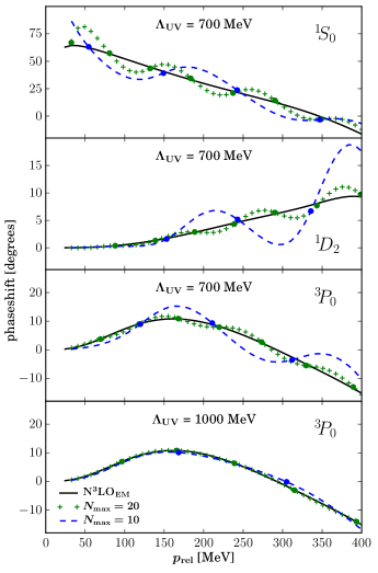
Figure 1: (Color online) Computed $np$ phase shifts of the $NN$ potential N³LO_EM Entem and Machleidt (2003) projected onto finite oscillator spaces with $N_{\rm max}$ = 10 and $N_{\rm max}$ = 20 compared to the phase shifts from the full (i.e., not projected) interaction in selected partial waves as a function of the relative momentum. In the top three panels the oscillator frequencies were chosen as $\hbar\omega$ = 40 MeV and 23 MeV, respectively, in order to obtain an oscillator cutoff $\Lambda_{\rm UV}\approx 700$ MeV that well exceeds the chiral cutoff $\Lambda_{\chi}=500$ MeV. The filled circles mark the phase shifts at the momenta corresponding to the eigenenergies of the scattering channel in the truncated oscillator space. In the bottom panel $\hbar\omega$ is increased to 80 MeV (for $N_{\rm max}=10$) and 46 MeV (for $N_{\rm max}=20$), respectively. This yields a UV cutoff $\Lambda_{\rm UV}\approx 1000$ MeV in the oscillator basis and significantly reduces the phase shift oscillations.

The projection onto finite oscillator bases introduces oscillations in the phase shifts. On the one hand, many ab initio calculations of atomic nuclei yield practically converged results for bound-state observables in model spaces with $N_{\rm max}\lesssim 14$ and oscillator frequencies around $24$ MeV. On the other hand, oscillator spaces consisting of only 10 to 20 shells are clearly too small to capture all the information contained in the original interaction. We note (i) that the N³LO_EM interaction is formulated for arbitrary continuous momenta whereas oscillator EFT limits the evaluation to a few discrete momenta, and (ii) that the present $\Lambda_{\rm UV}$ cuts off the high-momentum tails of the N³LO_EM interaction.

For $N_{\rm max}\rightarrow\infty$ we expect to arrive at the original phase shifts, and this is supported in Fig. 1 by the reduced oscillations in the $N_{\rm max}=20$ phase shifts compared to their $N_{\rm max}=10$ counterparts. The period of oscillations is approximately given by the IR cutoff. In the bottom panel of Fig. 1, the oscillator spacing $\hbar\omega$ is increased to 80 MeV (for $N_{\rm max}=10$) and 46 MeV (for $N_{\rm max}=20$), respectively, yielding a UV cutoff $\Lambda_{\rm UV}\approx 1000$ MeV in the oscillator basis. The phase shift oscillations are significantly reduced for such large values of $\Lambda_{\rm UV}$.

We note that the eigenvalues of the Hamiltonian matrix in $(N_{\rm max}+1)$ oscillator shells play a special role for the phase shifts in uncoupled partial wave channels. At these energies, the eigenfunctions are standing waves with a Dirichlet boundary condition at the (energy-dependent) radius of the spherical cavity that is equivalent to the finite oscillator basis, and one can alternatively use this information in the computation of the phase shifts Luu et al. (2010); More et al. (2013). The filled circles in Fig. 1 indicate the values of the phase shifts at these energies, which are close to those of the original interaction.

Subsection II.2 discusses two ways of projecting momentum-space interactions onto a finite oscillator space. The first approach involves the determination of the matrix element (31) via an exact numerical integration over continuous momenta. The second approach, Eq. (41), uses $(N+1)$-point Gauss-Laguerre quadrature to compute the integral in Eq. (31). This only requires us to evaluate the interaction at those momenta that are physically realized in the finite oscillator basis, which is more in the spirit of an EFT. Because we want to follow the oscillator EFT approach in later sections, we study the effect that the error term (34) associated with the $(N+1)$-point Gauss-Laguerre quadrature has on the projected phase shifts. Figure 2 shows a comparison of projected N³LO_EM phase shifts obtained from the two projection approaches to the original N³LO_EM phase shifts. Overall, both versions yield very similar phase shifts. For the phase shifts associated with the $(N+1)$-point Gauss-Laguerre quadrature, the oscillations seem to be somewhat reduced for small energies. Also, we find a notably improved agreement between the $(N+1)$-point Gauss-Laguerre phase shifts and the original ones at the discrete eigenenergies of the scattering channel Hamiltonians, as indicated by the full circles. From now on we exclusively use the $(N+1)$-point Gauss-Laguerre integration to compute matrix elements in oscillator EFT.

Figure 2: (Color online) Phase shifts of N³LO_EM obtained from a projection onto a $N_{\rm max}=10$, $\hbar\omega=40$ MeV oscillator space using (i) exact integration in Eq. (31) (blue, dashed line) and (ii) Gauss-Laguerre quadrature Eq. (41) (green crosses), compared to the unprojected N³LO_EM phase shifts (black, solid line). The filled circles mark the phase shifts at the momenta corresponding to the eigenenergies of the scattering channel in the truncated oscillator space.

III.2 Reproduction of the phase shifts of a NLO interaction

In what follows we employ the oscillator EFT at NLO. All matrix elements in oscillator EFT are based on Eq. (41), i.e., the matrix elements from continuum momentum space are evaluated at the discrete momenta of the finite oscillator basis. At this order the chiral interactions depend on 11 LECs and exhibit sufficient complexity to qualitatively describe nuclear properties. Specifically, in this Section we aim at reproducing the phase shifts and selected deuteron properties of the chiral interaction NLO_sim Carlsson et al. (2016) by optimizing these 11 LECs. Throughout this work, the $\chi^{2}$ fits evaluate the phase shifts at 20 equidistant energies in the laboratory energy range up to 350 MeV, with weights $\sigma^{2}\propto(q/\Lambda_{\chi})^{3}$. We note that more sophisticated weights (including also the pion mass or the oscillatory patterns) would be needed for a quantification of uncertainties, see, e.g. Refs. Stump et al. (2001); Carlsson et al. (2016); Furnstahl et al. (2015b). In this work we only investigate the feasibility of an oscillator EFT with regard to the computation of heavy nuclei.

The main goal of oscillator EFT is to enable the computation of heavy nuclei. Therefore, we set $N_{\rm max}=10$ for the interaction. This allows us to perform IR extrapolations based on calculations in spaces with $N_{\rm max}=10$, 12, and 14 for the kinetic energy. To determine $\hbar\omega$ we study phase shifts in selected partial waves in Fig. 3. The first value, $\hbar\omega=20$ MeV, again corresponds to a UV cutoff of $\Lambda_{\rm UV}\approx 500$ MeV and yields the familiar oscillations in the phase shifts. The second value, $\hbar\omega=34$ MeV, corresponds to a UV cutoff $\Lambda_{\rm UV}\approx 650$ MeV that significantly exceeds the chiral cutoff $\Lambda_{\chi}\approx 500$ MeV. In this case, the oscillations are drastically reduced. Consequently, we use $\hbar\omega=34$ MeV in the following.

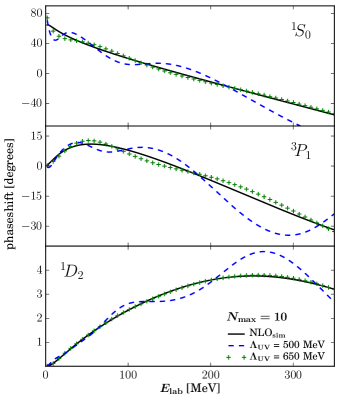
Figure 3: (Color online) Phase shifts of NLO interactions obtained from oscillator EFT through fits to $\text{NLO}_{\text{sim}}$ phase shifts compared to the $\text{NLO}_{\text{sim}}$ data Carlsson et al. (2016). The momentum-space interaction matrix elements used in the construction of the oscillator EFT interactions employ a fixed chiral cutoff $\Lambda_{\chi}=500$ MeV. We fix $N_{\rm max}=10$ and consider the two oscillator frequencies $\hbar\omega=20$ MeV and 34 MeV, yielding UV cutoffs $\Lambda_{\rm UV}=500$ MeV and 650 MeV, respectively. For $\Lambda_{\rm UV}=650$ MeV, the oscillations in the phase shifts are notably reduced.

In Fig. 4 we compare further phase shifts from the oscillator EFT to the $\text{NLO}_{\text{sim}}$ phase shifts. We note that the channel ${{}^{1}\!D_{2}}$ is a prediction because there is no corresponding LEC at this chiral order.

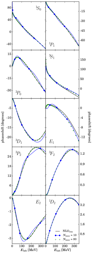
Figure 4: (Color online) Phase shifts from oscillator EFT with $N_{\rm max}=10$ (full blue circles and blue line) compared to NLO_sim phase shifts (black line) for partial wave channels as indicated. Also shown (green crosses) are results from oscillator EFT in a large model space with $N_{\rm max}=80$.

For completeness, and to assess the large-$N_{\rm max}$ behavior, we also show the results of an optimization in oscillator EFT with $N_{\rm max}=80$ and $\hbar\omega=6$ MeV ($\Lambda_{\rm UV}\approx 650$ MeV) as green crosses. In general, oscillator EFT reproduces the phase shifts well over the whole energy range up to the pion-production threshold.

	$N_{\rm max}=10$	$N_{\rm max}=80$	$\rm{NLO}_{\rm sim}$
$E_{d}\ [\text{MeV}]$	$-2.268$	$-2.212$	$-2.225$
$r_{d}\ \ [\text{fm}]$	$2.108$	$1.962$	$1.976$
$Q_{d}\ [\text{fm}^{2}]$	$0.195$	$0.259$	$0.259$
$P_{d}$	$0.028$	$0.029$	$0.029$
$\tilde{C}^{(np)}_{{}^{1}\!S_{0}}$	$-0.157499$	$-0.150552$	$-0.150623$
$\tilde{C}^{(pp)}_{{}^{1}\!S_{0}}$	$-0.15513$	$-0.14877$	$-0.14891$
$\tilde{C}^{(nn)}_{{}^{1}\!S_{0}}$	$-0.15645$	$-0.14990$	$-0.14991$
$C_{{}^{1}\!S_{0}}$	$1.7972$	$1.6910$	$1.6935$
$\tilde{C}_{{}^{3}\!S_{1}}$	$-0.1721$	$-0.1752$	$-0.1843$
$C_{{}^{3}\!S_{1}}$	$-0.406$	$-0.389$	$-0.218$
$C_{E_{1}}$	$0.224$	$0.232$	$0.263$
$C_{{}^{3}\!P_{0}}$	$1.3038$	$1.2995$	$1.2998$
$C_{{}^{1}\!P_{1}}$	$1.047$	$1.023$	$1.025$
$C_{{}^{3}\!P_{1}}$	$-0.335$	$-0.336$	$-0.336$
$C_{{}^{3}\!P_{2}}$	$-0.2010$	$-0.2028$	$-0.2029$

Table 1: Comparison of deuteron properties and LECs for effective interactions with $N_{\rm max}=10$, 80 obtained from a fit to NLO_sim phase shifts and deuteron properties, compared to NLO_sim data Carlsson et al. (2016). The deuteron properties, computed in large $N_{\rm max}=100$ model spaces, are the ground-state energy $E_{d}$, point-proton radius $r_{d}$, quadrupole moment $Q_{d}$, and $D$-state probability $P_{d}$. The oscillator frequencies $\hbar\omega$ are 34 MeV and 6 MeV, respectively, corresponding to a UV cutoff of $\Lambda_{\rm UV}\approx$ 650 MeV. Units of the LECs as in Ref. Machleidt and Entem (2011).

In the deuteron channel we fit not only to phase shifts but also to its binding energy $E_{d}$, point-proton radius $r_{d}$, and quadrupole moment $Q_{d}$. For $N_{\rm max}=80$, we reproduce the deuteron properties well, as can be seen in Table 1. For the $N_{\rm max}=10$ effective interaction, it becomes more difficult to simultaneously reproduce all data. Therefore, we relax the requirement to reproduce the quadrupole moment in favor of the other deuteron properties and the phase shifts. We converge the deuteron calculations by employing large model spaces of 100 oscillator shells where only the kinetic energy acts beyond the $N_{\rm max}$ used to define the effective interaction.

In Table 1 we also compare the LECs of the effective interactions for $N_{\rm max}$ = 10 and 80 to the LECs of NLO_sim. For $N_{\rm max}$ = 80, our approach quite accurately reproduces the NLO_sim LECs, with $C_{{}^{3}\!S_{1}}$ being the only exception. Because this LEC is associated with the deuteron channel, its value is affected by the weighting of the deuteron properties in the fit, and we expect that a better reproduction can be achieved by assigning different weights to the deuteron properties. More importantly, with the exception of $C_{{}^{3}\!S_{1}}$, the values of the LECs for the $N_{\rm max}$ = 10 interaction are very similar to the LECs of the NLO_sim interaction. Also, all of the values are of natural size.

Let us also address the sensitivity of our results to the UV cutoff of the employed oscillator space. For this purpose we keep $\hbar\omega=34$ MeV fixed and optimize two more interactions defined in model spaces with $N_{\rm max}=12$ and $N_{\rm max}=14$, respectively. We recall that the UV cutoff of the model space increases with increasing $N_{\rm max}$, and that $N_{\rm max}=10,12,14$ corresponds to UV cutoff $\Lambda_{\rm UV}\approx$ 650, 700, 750 MeV, respectively. Resulting few-body observables from these interactions are shown in Table 2, and also compared to the infinite-space interaction $\rm NLO_{sim}$. We see that results converge slowly toward those of the $\rm NLO_{sim}$ interaction as $N_{\rm max}$ is increased. We also note that the few-body observables from the different $N_{\rm max}$ interactions exhibit differences that are consistent with uncertainty expectations at NLO Epelbaum et al. (2015); Lynn et al. (2016); Carlsson et al. (2016).

	$N_{\rm max}=10$	$N_{\rm max}=12$	$N_{\rm max}=14$	$\rm NLO_{sim}$
$E_{d}$	-2.261	-2.227	-2.225	-2.224
$r_{d}$	2.108	1.974	1.889	1.975
$Q_{d}$	0.195	0.279	0.272	0.259
$P_{d}$	0.028	0.031	0.031	0.028
$E_{{}^{3}\text{H}}$	-8.944	-8.502	-8.094	-8.270
$r_{{}^{3}\text{H}}$	1.627	1.592	1.578	1.614
$E_{{}^{3}\text{He}}$	-8.169	-7.735	-7.33	-7.528
$r_{{}^{3}\text{He}}$	1.787	1.764	1.761	1.791
$E_{{}^{4}\text{He}}$	-28.736	-27.96	-27.302	-27.44
$r_{{}^{4}\text{He}}$	1.465	1.463	1.457	1.482

Table 2: Deuteron properties as in Table 1, as well as binding energies (in MeV) and radii (in fm) for ${}^{3}\rm H$, ${}^{3}\rm He$, and ${}^{4}\rm He$ from different effective interactions, compared to $\rm NLO_{sim}$. The oscillator length $\hbar\omega$ is fixed at 34 MeV, and we consider $N_{\rm max}$ = 10, 12, 14, corresponding to values of the UV cutoff $\Lambda_{\rm UV}\approx$ 650, 700, 750 MeV.

Clearly, the NLO interaction from oscillator EFT differs from NLO_sim through the complicated projection that introduces IR and UV cutoffs and is highly nonlocal, see Eq. (47). In the EFT sense the difference between these interactions should be beyond the order at which we are currently operating. While we cannot prove this equivalence, the numerical results of this Section encourage us to pursue the construction of a chiral NLO interaction within oscillator EFT by optimization to the phase shifts from a high-precision $NN$ potential in the following Section.

IV NLO interactions in oscillator EFT and many-body results

In what follows, we set $N_{\rm max}=10$ for the interaction. On the one hand, lower oscillator frequencies correspond to larger oscillator lengths and lead to a rapid IR convergence. On the other hand, lower oscillator frequencies also correspond to lower UV cutoffs. In what follows we choose $\hbar\omega=24$ MeV which results in a UV cutoff $\Lambda_{\rm UV}\approx 550$ MeV and an IR length $L\approx 9.6$ fm according to Eq. (22). Considering the tail of the regulator function (53) we set $\Lambda_{\chi}=450$ MeV, which ensures that $\Lambda_{\rm UV}$ significantly exceeds $\Lambda_{\chi}$.

Practical calculations are performed in the laboratory system, and use the $N_{\rm max}=10$ interaction together with the intrinsic kinetic energy in oscillator spaces with $N^{\rm lab}=2n_{1}+l_{1}\geq N_{\rm max}$. Here $n_{1}$ and $l_{1}$ are the radial and angular momentum quantum numbers of the harmonic oscillator in the laboratory frame. Results for $N^{\rm lab}=10,12,14$ are feasible and will allow us to perform IR extrapolations for bound-state energies and radii.

In this Section, we construct a chiral interaction at NLO from realistic phase shifts, and subsequently utilize it in coupled-cluster calculations of ⁴He, ¹⁶O, ⁴⁰Ca, ⁹⁰Zr, and ¹³²Sn. Our main objectives are (i) to present a proof-of-principle optimization of a realistic interaction within the framework of the oscillator EFT, and (ii) to demonstrate that such an interaction converges fast even in heavy nuclei. We compute the matrix elements in oscillator EFT, i.e., based on Eq. (41) and omit the high-order correction terms.

In the optimization, the low-energy coefficients are obtained from a $\chi^{2}$ fit to realistic scattering data (represented here by phase shifts from the CD-Bonn potential Machleidt (2001)) and deuteron properties. The fitting procedure is identical to the one described in Section III. Figure 5 presents the resulting phase shifts for a selection of scattering channels.

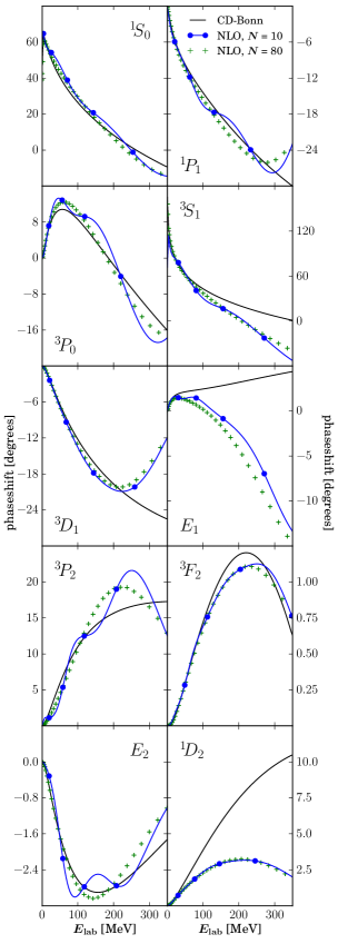
Figure 5: (Color online) Phase shift from oscillator EFT at NLO with $N_{\rm max}=10$ (full blue circles and blue line) compared to those of the CD Bonn interaction (full black line) for partial wave channels as indicated. The green crosses show results from a large model space with $N_{\rm max}=80$.

We reproduce the phase shifts over a large energy range for several partial waves. The ${{}^{1}\!D_{2}}$ channel is an obvious exception, as it deviates more clearly from the CD-Bonn phase shifts at higher energies, but we note that at NLO there is no LEC to adjust in this channel. For $E_{1}$, the deviations are also considerable, however, it is of NLO quality, see Fig. 4. For the deuteron, we obtain a good reproduction of the binding energy and radius, and a reasonably well result for the quadrupole moment, as shown in Table 3. The LECs, also shown in Table 3, are natural in size and similar to NLO_sim; the largest deviation is for the LEC $C_{{}^{1}\!P_{1}}$ which is only about $\nicefrac{{1}}{{3}}$ of its NLO_sim counterpart.

	$N_{\rm max}=10$	$N_{\rm max}=80$	experiment
$E_{d}\ [\text{MeV}]$	$-2.227$	$2.221$	$-2.225$
$r_{d}\ \ [\text{fm}]$	$1.984$	$1.961$	$1.976$
$Q_{d}\ [\text{fm}^{2}]$	$0.229$	$0.259$	$0.286$
$P_{d}$	$0.026$	$0.028$
$\tilde{C}^{(np)}_{{}^{1}\!S_{0}}$	$-0.140992$	$-0.139687$
$\tilde{C}^{(pp)}_{{}^{1}\!S_{0}}$	$-0.13991$	$-0.13855$
$\tilde{C}^{(nn)}_{{}^{1}\!S_{0}}$	$-0.14046$	$-0.13913$
$C_{{}^{1}\!S_{0}}$	$\hphantom{-}1.2470$	$\hphantom{-}1.2601$
$\tilde{C}_{{}^{3}\!S_{1}}$	$-0.1604$	$-0.1825$
$C_{{}^{3}\!S_{1}}$	$-0.682$	$-0.361$
$C_{E_{1}}$	$\hphantom{-}0.250$	$\hphantom{-}0.236$
$C_{{}^{3}\!P_{0}}$	$\hphantom{-}1.1629$	$\hphantom{-}1.1896$
$C_{{}^{1}\!P_{1}}$	$\hphantom{-}0.348$	$\hphantom{-}0.366$
$C_{{}^{3}\!P_{1}}$	$-0.336$	$-0.320$
$C_{{}^{3}\!P_{2}}$	$-0.1647$	$-0.1697$

Table 3: Deuteron properties (as in Table 1) and LECs from effective interactions in $N_{\rm max}=10$ and 80 shells obtained from a fit to CD-Bonn phase shifts and deuteron properties. The oscillator frequencies are $\hbar\omega$ = 24 MeV and 4 MeV for $N_{\rm max}$ = 10 and 80, respectively.

We utilize the NLO interaction in coupled-cluster calculations at the singles and doubles level (CCSD) Kümmel et al. (1978); Shavitt and Bartlett (2009); Hagen et al. (2014) of the nuclei ⁴He, ¹⁶O, ⁴⁰Ca, ⁹⁰Zr, and ¹³²Sn. The coupled-cluster calculations use Hartree-Fock bases that are unitarily equivalent to the oscillator bases but lead to improved results. In these calculations, we keep the oscillator spacing fixed at $\hbar\omega=24$ MeV in the spirit of oscillator EFT. We employ model spaces from $N^{\rm lab}=10$ up to $N^{\rm lab}=16$. In the oscillator basis, the potential is always restricted to $N_{\rm max}=10$, while the kinetic energy is used in the entire model space. The results are shown in Table 4. The $N^{\rm lab}=16$ point is used to gauge convergence of the results. For the light nuclei, energies and radii are practically IR converged already for $N^{\rm lab}=10$ because $r^{2}\ll L^{2}$.

$N^{\rm lab}$	${}^{4}\rm{He}$	${}^{16}\rm{O}$	${}^{40}\rm{Ca}$	${}^{90}\rm{Zr}$	${}^{132}\rm{Sn}$
	$E_{\rm CCSD}$ [MeV]
10	-31.57	-142.89	-402.0	-918.4	-1230.0
12	-31.57	-142.92	-402.4	-923.1	-1249.3
14	-31.57	-142.93	-402.5	-924.6	-1255.6
16	-31.57	-142.93	-402.5	-925.1	-1258.3
$\infty$	-31.57	-142.93	-402.5	-925.4	-1260.1
exp	-28.30	-127.62	-342.1	-783.9	-1102.9
	$r^{2}\ \rm[fm^{2}]$
10	1.78	4.14	6.58	9.70	11.60
12	1.78	4.15	6.60	9.77	11.79
14	1.78	4.15	6.60	9.80	11.85
16	1.78	4.15	6.61	9.82	11.88
$\infty$	1.78	4.15	6.61	9.83	11.89
exp	2.12	6.60	11.41	17.57	21.57

Table 4: Ground-state energies $E_{\rm CCSD}$ and squared point-proton radii $r^{2}$ for nuclei ranging from ⁴He to ¹³²Sn from CCSD calculations in many-body model spaces built from single-particle oscillator bases with $N^{\rm lab}=10,\dots,16$. In the relative frame the oscillator EFT interaction is defined in the $N_{\rm max}=10$ model space, and the Hamiltonian matrix elements outside this space are comprised of the kinetic energy only. Experimental data taken from Wang et al. (2012); Angeli and Marinova (2013). The experimental point-proton radii are extracted from charge radii by correcting for the finite sizes of the proton and neutron, and the Darwin-Foldy term.

The convergence with respect to $N^{\rm lab}$ is very fast compared to other interactions from chiral EFT with a cutoff of around $\Lambda_{\chi}\approx 450$ MeV Roth et al. (2014). For IR extrapolations of ground-state energies $E$ we employ Furnstahl et al. (2012)

$$E(L)=E_{\infty}+ae^{-2k_{\infty}L},$$ (55)

where $L\approx\sqrt{2(N^{\rm lab}+\nicefrac{{7}}{{2}})}b$ is the IR length More et al. (2013). In the fit, we employ a theoretical uncertainty $\sigma\equiv\exp{(-2k_{\infty}L)/(k_{\infty}L)}$ to account for omitted corrections beyond the leading-order result (55). The difference between the IR extrapolated energies and the energy at $N^{\rm lab}=16$ is much smaller than both, the uncertainty of about 7% in correlation energy due to the CCSD approximation, and the uncertainty expected from higher orders in the chiral expansion.

Figure 6 (top) shows the result of an IR extrapolation for the ground-state energy of ¹³²Sn. Here, we plotted energies in $N^{\rm lab}=10$ to 16 as a function of the IR length $L$ and also show the exponential IR extrapolation Furnstahl et al. (2012) The inset of Fig. 6 confirms the exponential convergence of the energy.

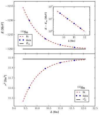
Figure 6: (Color online) IR convergence of the ground-state energy (top) and squared radius (bottom) of ¹³²Sn computed from CCSD calculations using the oscillator EFT interaction. Data is shown as blue points, the extrapolations as red dashed lines, and the asymptotic energy and radius as solid black lines. The inset on the top shows that the ground-state energy is approached exponentially in the IR length $L$.

Figure 6 (bottom) shows the results of an IR extrapolation for the ground-state expectation value of the squared radius of ¹³²Sn. We plotted squared point-proton radii in model spaces with $N^{\rm lab}=10$ to 16 as a function of the IR length $L$ and performed a $\chi^{2}$ fit to the IR extrapolation Furnstahl et al. (2012)

$$r^{2}(L)=r_{\infty}^{2}-b(k_{\infty}L)^{3}e^{-2k_{\infty}L}.$$ (56)

In the $\chi^{2}$ fit of the radius, we refit the constant $k_{\infty}$ and employed theoretical uncertainties $\sigma\equiv k_{\infty}L\exp{(-2k_{\infty}L)}$ to account for corrections to the leading-order result (56). Numerical results for the radii are listed in Table 4. The results from IR extrapolations involving only the data points from $N^{\rm lab}=10$ to 14 yield $E_{\infty}=-1259.2$ MeV and $r_{\infty}^{2}=11.88$ fm² for ¹³²Sn, which are close to the previous results including the $N^{\rm lab}=16$ points.

The oscillator EFT interaction at NLO overbinds nuclei by about 1 MeV per nucleon, and radii are too small. We note that the difference between theoretical and experimental values for the ground-state energies seem to be consistent with expectations from an NLO interaction. We also note that three-nucleon forces entering at next-to-next-to-leading order will be part of the saturation mechanism Hebeler et al. (2011); Ekström et al. (2015).

The rapid convergence of ground-state energies and radii in oscillator EFT suggests that chiral cutoffs of $\Lambda_{\chi}\approx 450$ MeV are reasonable in nuclear-structure computations of heavy nuclei. Similar to renormalization group transformations the oscillator EFT reduces the mismatch between the tail of the momentum-space regulator and the oscillator space.

V Summary

We developed an EFT directly in the oscillator basis. In this approach UV convergence is implemented by construction, and IR convergence can be achieved by enlarging the model space for the kinetic energy only. We discussed practical aspects of the oscillator EFT and gave analytical expressions for the efficient calculation of matrix elements in oscillator EFT from their continuous-momentum counterparts. Within the $J$-matrix approach we computed phase shifts while working exclusively in the oscillator basis. Our results suggest that oscillations in the phase shifts appear when the UV cutoff imposed by the oscillator basis cuts into the high-momentum tails of the chiral interaction. To validate the oscillator EFT approach we reproduced a chiral interaction at NLO. Finally, we developed a chiral NLO interaction in oscillator EFT by optimizing the LECs to CD-Bonn phase shifts and experimental deuteron data. Coupled-cluster calculations for nuclei from ⁴He up to ¹³²Sn exhibit a rapid convergence for ground-state energies and radii. These results suggest that the oscillator EFT is a promising candidate to facilitate ab initio calculations of heavy atomic nuclei based on interactions from chiral EFT using currently available many-body methods.

*

Appendix A Matrix elements in oscillator EFT

In this Appendix we give an alternative motivation for the computation (41) of matrix elements in oscillator EFT. These results are well known for DVRs, see, e.g., Ref. Littlejohn et al. (2002). The projection onto a finite oscillator space is based on the usual scalar product

$$\langle\tilde{\Psi}_{f}|\tilde{\Psi}_{g}\rangle=\int\limits_{0}^{\infty}{\rm d}kk^{2}\tilde{\Psi}_{f}(k)\tilde{\Psi}_{g}(k)$$ (57)

for radial wave functions in momentum space. The projection operator onto the finite oscillator space at fixed angular momentum $l$ is

$$\hat{\Pi}_{l}\equiv\sum_{\nu=0}^{N}|\phi_{\nu,l}\rangle\langle\phi_{\nu,l}|.$$ (58)

Let us alternatively consider a different projection operator, which is based on a different scalar product. We write momentum-space wave functions with angular momentum $l$ as

$$\tilde{\Psi}_{f}(k)=\sqrt{2b^{3}}(kb)^{l}e^{-{1\over 2}(kb)^{2}}f(k^{2}b^{2}).$$ (59)

Here, $f(x)$ is a polynomial in $x=k^{2}b^{2}$. It is clear that any square-integrable wave function can be built from such polynomials (with Laguerre polynomials $L_{n}^{l+\nicefrac{{1}}{{2}}}$ being an example). We define the (semi-definite) scalar product $(\cdot|\cdot)$ of two functions $\tilde{\Psi}_{f}$ and $\tilde{\Psi}_{g}$ as

$$(\tilde{\Psi}_{f}|\tilde{\Psi}_{g})\equiv\sum_{\mu=0}^{N}w_{\mu,l}f(x_{\mu,l})g(x_{\mu,l}).$$ (60)

Here, the weights are from Eq. (33) and the abscissas $x_{\mu,l}\equiv k_{\mu,l}^{2}b^{2}$ are the zeros of the associated Laguerre polynomial $L_{N+1}^{l+\nicefrac{{1}}{{2}}}$ as demanded by $(N+1)$-point Gauss-Laguerre quadrature. Equation (60) defines only a semi-definite inner product, because $(\tilde{\Psi}_{f}|\tilde{\Psi}_{f})=0$ for any polynomial $f$ with $f(x_{\mu,l})=0$ for $\mu=0,\dots,N$.

Several comments are in order. First, this semi-definite scalar product is identical to the standard scalar product (57) for wave functions $\tilde{\Psi}_{f}(k)$ that are limited to the finite oscillator space. To see this, we note that

$$\langle\tilde{\Psi}_{f}|\tilde{\Psi}_{g}\rangle = \int\limits_{0}^{\infty}{\rm d}kk^{2}\tilde{\Psi}_{f}(k)\tilde{\Psi}_{g}(k)$$ (61)

$$= \int\limits_{0}^{\infty}{\rm d}xx^{l+\nicefrac{{1}}{{2}}}e^{-x}f(x)g(x)$$

$$= \sum_{\mu=0}^{N}w_{\mu,l}f(x_{\mu,l})g(x_{\mu,l}).$$

Here, we introduced the dimensionless integration variable $x\equiv k^{2}b^{2}$ in the second line and employ $(N+1)$-point Gauss-Laguerre quadrature in the third line. We note that $(N+1)$-point Gauss-Laguerre quadrature is exact for polynomials of degree up to and including $2N+1$, i.e., it is exact for polynomials $f,g$ spanned by $L_{n}^{l+\nicefrac{{1}}{{2}}}(x)$ with $n=0,\ldots,N$.

This implies that the basis functions $\tilde{\psi}_{n,l}(k)$ with $n=0,\ldots,N$ in the finite oscillator space remain a basis under the semi-definite scalar product, i.e.

$$(\tilde{\psi}_{n,l}|\tilde{\psi}_{n^{\prime},l})=\delta_{n}^{n^{\prime}}.$$ (62)

Second, we note that both scalar products also agree for $N\to\infty$ because Gauss-Laguerre integration becomes exact in this limit.

Rewriting the weights $w_{\nu,l}$ in Eq. (33) as

$$w_{\nu,l} = \frac{2b^{3}(k_{\nu,l}b)^{2}(k_{\nu,l}b)^{2l}e^{-(k^{2}_{\nu,l}b^{2})}}{(N+1)(N+l+\nicefrac{{3}}{{2}})\left[\tilde{\psi}_{N,l}(k_{\nu,l})\right]^{2}}$$ (63)

$$= 2b^{3}(k_{\nu,l}b)^{l}e^{-{1\over 2}(k^{2}_{\nu,l}b^{2})}c_{\nu,l}^{2},$$

and using Eq. (25) yields another useful expression for the scalar product (60)

$$(\tilde{\Psi}_{f}|\tilde{\Psi}_{g}) = \sum_{\mu=0}^{N}c_{\mu,l}^{2}\tilde{\Psi}_{f}(k_{\mu,l})\tilde{\Psi}_{g}(k_{\mu,l}).$$ (64)

A main difference between the scalar products of Eq. (57) and Eq. (64) arises when one compares the wave function

$$\langle k,l|\phi_{\nu,l}\rangle=\tilde{\phi}_{\nu,l}(k)$$ (65)

of Eq. (27) with the corresponding scalar product

$$(k,l|\tilde{\phi}_{\nu,l}) = \sum_{\mu=0}^{N}c_{\mu,l}^{2}{\delta(k-k_{\mu,l})\over k^{2}}\tilde{\phi}_{\nu,l}(k_{\nu,l})$$ (66)

$$= c_{\nu,l}{\delta(k-k_{\nu,l})\over k_{\nu,l}^{2}}.$$

Here, we used Eq. (64) and Eq. (27) implying $\tilde{\phi}_{\mu,l}(k_{\lambda,l})=c_{\lambda,l}^{-1}\delta_{\mu}^{\lambda}$. Clearly, the Fourier-Bessel transform (27) of the discrete momentum eigenstate $\phi_{\nu,l}$ has a complicated momentum dependence, while $(k,l|\tilde{\phi}_{\nu,l})$ is simply a rescaled $\delta$ function. This simple view is consistent with naive expectation of a momentum eigenstate.

We are now in the position to compute matrix elements based on the inner product (60). We note that

$$\hat{V}|\phi_{\mu,l}) = \hat{V}\int\limits_{0}^{\infty}{\rm d}kk^{2}|k,l\rangle(k,l|\phi_{\mu,l})$$ (67)

$$= \hat{V}|k_{\mu,l}\rangle c_{\mu,l}.$$

Here, we used Eq. (66). Repeating the procedure on the bra side yields

$$(\phi_{\nu,l^{\prime}}|\hat{V}|\phi_{\mu,l})=\langle k_{\nu,l^{\prime}},l^{\prime}|\hat{V}|k_{\mu,l},l\rangle c_{\nu,l^{\prime}}c_{\mu,l},$$ (68)

and this is Eq. (41). We repeat that this derivation of the interaction matrix element is based on the scalar product (64) and not on the usual scalar product (57) for square integrable functions. We argue that the former scalar product is more natural considering the discrete momentum mesh that is employed in oscillator EFT.

For another view on the semi-definite scalar product we consider the projection operator

$$\hat{P}_{l}\equiv\sum_{n=0}^{N}|\tilde{\psi}_{n,l})(\tilde{\psi}_{n,l}|.$$ (69)

Indeed, $\hat{P}_{l}^{2}=\hat{P}_{l}$. This makes it interesting to consider the projected wave function

$$\left(\hat{P}_{l}\tilde{\Psi}_{f}\right)(k_{\mu,l}) = \sum_{n=0}^{N}(\tilde{\psi}_{n,l}|\tilde{\Psi}_{f})\tilde{\psi}_{n,l}(k_{\mu,l})$$ (70)

$$= \sum_{\nu=0}^{N}c_{\nu,l}^{2}\tilde{\Psi}_{f}(k_{\nu,l})\sum_{n=0}^{N}\tilde{\psi}_{n,l}(k_{\nu,l})\tilde{\psi}_{n,l}(k_{\mu,l})$$

$$= \tilde{\Psi}_{f}(k_{\mu,l}).$$

Here, we evaluated the sum over $n$ using Eq. (29) when going from the second to the third line. Equation (70) shows that the projected wave function agrees with the full wave function at the discrete momenta $k_{\mu,l}$. In other words, the projection based on the semi-definite scalar product yields wave functions in finite oscillator spaces that agree with the unprojected wave functions at the physical momenta.

Let us give another interpretation of the projection $\hat{P}_{l}$. One finds for the scalar product (64)

$$(\tilde{\Psi}_{f}|\tilde{\Psi}_{g})=\sum_{\mu=0}^{N}c_{\mu,l}^{2}\tilde{\Psi}_{f}(k_{\mu,l})\tilde{\Psi}_{g}(k_{\mu,l})$$ (71)

$$= \langle\tilde{\Psi}_{f}|\left(\sum_{\mu=0}^{N}|k_{\mu,l},l\rangle c_{\mu,l}^{2}\langle k_{\mu,l},l|\right)|\tilde{\Psi}_{g}\rangle.$$

Thus, the scalar product $(\tilde{\Psi}_{f}|\tilde{\Psi}_{g})$ can be viewed as a matrix element of the operator in the brackets.

References

- Epelbaum et al. (2009) E. Epelbaum, H.-W. Hammer, and Ulf-G. Meißner, “Modern theory of nuclear forces,” Rev. Mod. Phys. 81, 1773–1825 (2009).
- Machleidt and Entem (2011) R. Machleidt and D.R. Entem, “Chiral effective field theory and nuclear forces,” Physics Reports 503, 1 – 75 (2011).
- Maris et al. (2009) P. Maris, J. P. Vary, and A. M. Shirokov, “Ab initio no-core full configuration calculations of light nuclei,” Phys. Rev. C 79, 014308 (2009).
- Hagen et al. (2010) G. Hagen, T. Papenbrock, D. J. Dean, and M. Hjorth-Jensen, “Ab initio coupled-cluster approach to nuclear structure with modern nucleon-nucleon interactions,” Phys. Rev. C 82, 034330 (2010).
- Jurgenson et al. (2013) E. D. Jurgenson, P. Maris, R. J. Furnstahl, P. Navrátil, W. E. Ormand, and J. P. Vary, “Structure of -shell nuclei using three-nucleon interactions evolved with the similarity renormalization group,” Phys. Rev. C 87, 054312 (2013).
- Roth et al. (2014) Robert Roth, Angelo Calci, Joachim Langhammer, and Sven Binder, “Evolved chiral hamiltonians for ab initio nuclear structure calculations,” Phys. Rev. C 90, 024325 (2014).
- Bogner et al. (2003) S. K. Bogner, T. T. S. Kuo, and A. Schwenk, “Model-independent low momentum nucleon interaction from phase shift equivalence,” Physics Reports 386, 1 – 27 (2003).
- Bogner et al. (2007) S. K. Bogner, R. J. Furnstahl, and R. J. Perry, “Similarity renormalization group for nucleon-nucleon interactions,” Phys. Rev. C 75, 061001 (2007).
- Jurgenson et al. (2009) E. D. Jurgenson, P. Navrátil, and R. J. Furnstahl, “Evolution of nuclear many-body forces with the similarity renormalization group,” Phys. Rev. Lett. 103, 082501 (2009).
- Lisetskiy et al. (2009) A. F. Lisetskiy, M. K. G. Kruse, B. R. Barrett, P. Navratil, I. Stetcu, and J. P. Vary, “Effective operators from exact many-body renormalization,” Phys. Rev. C 80, 024315 (2009).
- Schuster et al. (2014) Micah D. Schuster, Sofia Quaglioni, Calvin W. Johnson, Eric D. Jurgenson, and Petr Navrátil, “Operator evolution for ab initio theory of light nuclei,” Phys. Rev. C 90, 011301 (2014).
- Lee (2009) Dean Lee, “Lattice simulations for few- and many-body systems,” Progress in Particle and Nuclear Physics 63, 117 – 154 (2009).
- Lüscher (1986) M. Lüscher, “Volume Dependence of the Energy Spectrum in Massive Quantum Field Theories. 1. Stable Particle States,” Commun. Math. Phys. 104, 177 (1986).
- Navrátil et al. (2009) Petr Navrátil, Sofia Quaglioni, Ionel Stetcu, and Bruce R Barrett, “Recent developments in no-core shell-model calculations,” Journal of Physics G 36, 083101 (2009).
- Barrett et al. (2013) Bruce R. Barrett, Petr Navrátil, and James P. Vary, “Ab initio no core shell model,” Progress in Particle and Nuclear Physics 69, 131 – 181 (2013).
- Hagen et al. (2012) G. Hagen, M. Hjorth-Jensen, G. R. Jansen, R. Machleidt, and T. Papenbrock, “Evolution of shell structure in neutron-rich calcium isotopes,” Phys. Rev. Lett. 109, 032502 (2012).
- Holt et al. (2012) Jason D. Holt, Takaharu Otsuka, Achim Schwenk, and Toshio Suzuki, “Three-body forces and shell structure in calcium isotopes,” Journal of Physics G 39, 085111 (2012).
- Wienholtz et al. (2013) F. Wienholtz, D. Beck, K. Blaum, Ch. Borgmann, M. Breitenfeldt, R. B. Cakirli, S. George, F. Herfurth, J. D. Holt, M. Kowalska, S. Kreim, D. Lunney, V. Manea, J. Menendez, D. Neidherr, M. Rosenbusch, L. Schweikhard, A. Schwenk, J. Simonis, J. Stanja, R. N. Wolf, and K. Zuber, “Masses of exotic calcium isotopes pin down nuclear forces,” Nature 498, 346–349 (2013).
- Somà et al. (2014) V. Somà, A. Cipollone, C. Barbieri, P. Navrátil, and T. Duguet, “Chiral two- and three-nucleon forces along medium-mass isotope chains,” Phys. Rev. C 89, 061301 (2014).
- Lähde et al. (2014) T. A. Lähde, E. Epelbaum, H. Krebs, D. Lee, U.-G. Meißner, and G. Rupak, “Lattice effective field theory for medium-mass nuclei,” Phys. Lett. B 732, 110 – 115 (2014).
- Hagen et al. (2014) G. Hagen, T. Papenbrock, M. Hjorth-Jensen, and D. J. Dean, “Coupled-cluster computations of atomic nuclei,” Reports on Progress in Physics 77, 096302 (2014).
- Hergert et al. (2014) H. Hergert, S. K. Bogner, T. D. Morris, S. Binder, A. Calci, J. Langhammer, and R. Roth, “Ab initio multireference in-medium similarity renormalization group calculations of even calcium and nickel isotopes,” Phys. Rev. C 90, 041302 (2014).
- Hagen et al. (2016) G. Hagen, A. Ekström, C. Forssén, G. R. Jansen, W. Nazarewicz, T. Papenbrock, K. A. Wendt, S. Bacca, N. Barnea, B. Carlsson, C. Drischler, K. Hebeler, M. Hjorth-Jensen, M. Miorelli, G. Orlandini, A. Schwenk, and J. Simonis, “Neutron and weak-charge distributions of the 48Ca nucleus,” Nature Physics 12, 186 (2016).
- Binder et al. (2014) Sven Binder, Joachim Langhammer, Angelo Calci, and Robert Roth, “Ab initio path to heavy nuclei,” Physics Letters B 736, 119 – 123 (2014).
- Ekström et al. (2013) A. Ekström, G. Baardsen, C. Forssén, G. Hagen, M. Hjorth-Jensen, G. R. Jansen, R. Machleidt, W. Nazarewicz, T. Papenbrock, J. Sarich, and S. M. Wild, “Optimized chiral nucleon-nucleon interaction at next-to-next-to-leading order,” Phys. Rev. Lett. 110, 192502 (2013).
- Ekström et al. (2015) A. Ekström, G. R. Jansen, K. A. Wendt, G. Hagen, T. Papenbrock, B. D. Carlsson, C. Forssén, M. Hjorth-Jensen, P. Navrátil, and W. Nazarewicz, “Accurate nuclear radii and binding energies from a chiral interaction,” Phys. Rev. C 91, 051301 (2015).
- Carlsson et al. (2016) B. D. Carlsson, A. Ekström, C. Forssén, D. Fahlin Strömberg, G. R. Jansen, O. Lilja, M. Lindby, B. A. Mattsson, and K. A. Wendt, “Uncertainty analysis and order-by-order optimization of chiral nuclear interactions,” Phys. Rev. X 6, 011019 (2016).
- Entem et al. (2015) D. R. Entem, N. Kaiser, R. Machleidt, and Y. Nosyk, “Peripheral nucleon-nucleon scattering at fifth order of chiral perturbation theory,” Phys. Rev. C 91, 014002 (2015).
- Epelbaum et al. (2015) E. Epelbaum, H. Krebs, and U.-G. Meißner, “Precision nucleon-nucleon potential at fifth order in the chiral expansion,” Phys. Rev. Lett. 115, 122301 (2015).
- Gezerlis et al. (2014) A. Gezerlis, I. Tews, E. Epelbaum, M. Freunek, S. Gandolfi, K. Hebeler, A. Nogga, and A. Schwenk, “Local chiral effective field theory interactions and quantum monte carlo applications,” Phys. Rev. C 90, 054323 (2014).
- Haxton and Song (2000) W. C. Haxton and C.-L. Song, “Morphing the shell model into an effective theory,” Phys. Rev. Lett. 84, 5484–5487 (2000).
- Haxton and Luu (2002) W. C. Haxton and T. Luu, “Perturbative effective theory in an oscillator basis?” Phys. Rev. Lett. 89, 182503 (2002).
- Haxton (2007) W. C. Haxton, “Harmonic-oscillator-based effective theory,” in Opportunities with Exotic Beams (World Scientific, 2007) Chap. 13, pp. 117–131.
- Haxton (2008) W. C. Haxton, “Form of the effective interaction in harmonic-oscillator-based effective theory,” Phys. Rev. C 77, 034005 (2008).
- Stetcu et al. (2007) I. Stetcu, B.R. Barrett, and U. van Kolck, “No-core shell model in an effective-field-theory framework,” Physics Letters B 653, 358 – 362 (2007).
- Stetcu et al. (2010) I. Stetcu, J. Rotureau, B. R. Barrett, and U. van Kolck, “Effective interactions for light nuclei: an effective (field theory) approach,” Journal of Physics G 37, 064033 (2010).
- Rotureau et al. (2012) J. Rotureau, I. Stetcu, B. R. Barrett, and U. van Kolck, “Two and three nucleons in a trap, and the continuum limit,” Phys. Rev. C 85, 034003 (2012).
- Rotureau et al. (2010) J. Rotureau, I. Stetcu, B. R. Barrett, M. C. Birse, and U. van Kolck, “Three and four harmonically trapped particles in an effective-field-theory framework,” Phys. Rev. A 82, 032711 (2010).
- Tölle et al. (2011) S. Tölle, H.-W. Hammer, and B. Ch. Metsch, “Universal few-body physics in a harmonic trap,” Comptes Rendus Physique 12, 59 – 70 (2011).
- Tölle et al. (2013) S. Tölle, H.-W. Hammer, and B. Ch. Metsch, “Convergence properties of the effective theory for trapped bosons,” Journal of Physics G 40, 055004 (2013).
- Heller and Yamani (1974) Eric J. Heller and Hashim A. Yamani, “New approach to quantum scattering: Theory,” Phys. Rev. A 9, 1201–1208 (1974).
- Shirokov et al. (2004) A. M. Shirokov, A. I. Mazur, S. A. Zaytsev, J. P. Vary, and T. A. Weber, “Nucleon-nucleon interaction in the -matrix inverse scattering approach and few-nucleon systems,” Phys. Rev. C 70, 044005 (2004).
- Coon et al. (2012) S. A. Coon, M. I. Avetian, M. K. G. Kruse, U. van Kolck, P. Maris, and J. P. Vary, “Convergence properties of ab initio calculations of light nuclei in a harmonic oscillator basis,” Phys. Rev. C 86, 054002 (2012).
- Furnstahl et al. (2012) R. J. Furnstahl, G. Hagen, and T. Papenbrock, “Corrections to nuclear energies and radii in finite oscillator spaces,” Phys. Rev. C 86, 031301 (2012).
- More et al. (2013) S. N. More, A. Ekström, R. J. Furnstahl, G. Hagen, and T. Papenbrock, “Universal properties of infrared oscillator basis extrapolations,” Phys. Rev. C 87, 044326 (2013).
- Furnstahl et al. (2014) R. J. Furnstahl, S. N. More, and T. Papenbrock, “Systematic expansion for infrared oscillator basis extrapolations,” Phys. Rev. C 89, 044301 (2014).
- König et al. (2014) S. König, S. K. Bogner, R. J. Furnstahl, S. N. More, and T. Papenbrock, “Ultraviolet extrapolations in finite oscillator bases,” Phys. Rev. C 90, 064007 (2014).
- Furnstahl et al. (2015a) R. J. Furnstahl, G. Hagen, T. Papenbrock, and K. A. Wendt, “Infrared extrapolations for atomic nuclei,” Journal of Physics G 42, 034032 (2015a).
- Wendt et al. (2015) K. A. Wendt, C. Forssén, T. Papenbrock, and D. Sääf, “Infrared length scale and extrapolations for the no-core shell model,” Phys. Rev. C 91, 061301 (2015).
- Shirokov et al. (2007) A.M. Shirokov, J.P. Vary, A.I. Mazur, and T.A. Weber, “Realistic nuclear hamiltonian: Ab exitu approach,” Physics Letters B 644, 33 – 37 (2007).
- Harris et al. (1965) D. O. Harris, G. G. Engerholm, and W. D. Gwinn, “Calculation of matrix elements for one -dimensional quantum- mechanical problems and the application to anharmonic oscillators,” J. Chem. Phys. 43, 1515–1517 (1965).
- Dickinson and Certain (1968) A. S. Dickinson and P. R. Certain, “Calculation of matrix elements for one- dimensional quantum- mechanical problems,” J. Chem. Phys. 49, 4209–4211 (1968).
- Light et al. (1985) J. C. Light, I. P. Hamilton, and J. V. Lill, “Generalized discrete variable approximation in quantum mechanics,” J. Chem. Phys. 82, 1400–1409 (1985).
- Baye and Heenen (1986) D. Baye and P.-H. Heenen, “Generalised meshes for quantum mechanical problems,” J. Physics A: Math. Gen. 19, 2041 (1986).
- Littlejohn et al. (2002) R. G. Littlejohn, M. Cargo, T. Carrington, K. A. Mitchell, and B. Poirier, “A general framework for discrete variable representation basis sets,” J. Chem. Phys. 116, 8691–8703 (2002).
- Light and Carrington (2007) J. C. Light and T. Carrington, “Discrete-variable representations and their utilization,” in Adv. Chem. Phys. (John Wiley & Sons, Inc., 2007) pp. 263–310.
- Bulgac and McNeil Forbes (2013) A. Bulgac and M. McNeil Forbes, “Use of the discrete variable representation basis in nuclear physics,” Phys. Rev. C 87, 051301 (2013).
- Gradshteyn and Ryzhik (2000) L. S. Gradshteyn and L. M. Ryzhik, Tables of integrals, series, and products, 6th ed. (Academic Press, San Diego, 2000).
- Concus et al. (1963) P. Concus, D. Cassatt, G. Jaehnig, and E. Melby, “Tables for the evaluation of by Gauss-Laguerre quadrature,” Math. Comp. 17, 245–256 (1963).
- Entem and Machleidt (2003) D. R. Entem and R. Machleidt, “Accurate charge-dependent nucleon-nucleon potential at fourth order of chiral perturbation theory,” Phys. Rev. C 68, 041001 (2003).
- Luu et al. (2010) Thomas Luu, Martin J. Savage, Achim Schwenk, and James P. Vary, “Nucleon-nucleon scattering in a harmonic potential,” Phys. Rev. C 82, 034003 (2010).
- Stump et al. (2001) D. Stump, J. Pumplin, R. Brock, D. Casey, J. Huston, J. Kalk, H. L. Lai, and W. K. Tung, “Uncertainties of predictions from parton distribution functions. i. the lagrange multiplier method,” Phys. Rev. D 65, 014012 (2001).
- Furnstahl et al. (2015b) R. J. Furnstahl, N. Klco, D. R. Phillips, and S. Wesolowski, “Quantifying truncation errors in effective field theory,” Phys. Rev. C 92, 024005 (2015b).
- Lynn et al. (2016) J. E. Lynn, I. Tews, J. Carlson, S. Gandolfi, A. Gezerlis, K. E. Schmidt, and A. Schwenk, “Chiral three-nucleon interactions in light nuclei, neutron- scattering, and neutron matter,” Phys. Rev. Lett. 116, 062501 (2016).
- Machleidt (2001) R. Machleidt, “High-precision, charge-dependent Bonn nucleon-nucleon potential,” Phys. Rev. C 63, 024001 (2001).
- Kümmel et al. (1978) H. Kümmel, K. H. Lührmann, and J. G. Zabolitzky, “Many-fermion theory in expS- (or coupled cluster) form,” Physics Reports 36, 1 – 63 (1978).
- Shavitt and Bartlett (2009) I. Shavitt and R. J. Bartlett, Many-body Methods in Chemistry and Physics (Cambridge University Press, 2009).
- Wang et al. (2012) M. Wang, G. Audi, A.H. Wapstra, F.G. Kondev, M. MacCormick, X. Xu, and B. Pfeiffer, “The AME 2012 atomic mass evaluation,” Chinese Physics C 36, 1603 (2012).
- Angeli and Marinova (2013) I. Angeli and K.P. Marinova, “Table of experimental nuclear ground state charge radii: An update,” At. Data Nucl. Data Tables 99, 69 – 95 (2013).
- Hebeler et al. (2011) K. Hebeler, S. K. Bogner, R. J. Furnstahl, A. Nogga, and A. Schwenk, “Improved nuclear matter calculations from chiral low-momentum interactions,” Phys. Rev. C 83, 031301 (2011).