Strengthening the SDP Relaxation of AC Power Flows with
Convex Envelopes, Bound Tightening, and Lifted Nonlinear Cuts

Abstract

This paper considers state-of-the-art convex relaxations for the AC power flow equations and introduces valid cuts based on convex envelopes and lifted nonlinear constraints. These valid linear inequalities strengthen existing semidefinite and quadratic programming relaxations and dominate existing cuts proposed in the literature. Combined with model intersection and bound tightening, the new linear cuts close 8 of the remaining 16 open test cases in the NESTA archive for the AC Optimal Power Flow problem.

Nomenclature

$N$

- The set of nodes in the network

$E$

- The set of from edges in the network

$\bm{i}$

- imaginary number constant

$I$

- AC current

$S=p+\bm{i}q$

- AC power

$V=v\angle\theta$

- AC voltage

$Z=r+\bm{i}x$

- Line impedance

$Y=g+\bm{i}b$

- Line admittance

$W=w^{R}+\bm{i}w^{I}$

- Product of two AC voltages

$s^{u}$

- Line apparent power thermal limit

$\theta_{ij}$

- Phase angle difference (i.e. $\theta_{i}-\theta_{j}$)

$\phi$

- Phase angle difference center

$\delta$

- Phase angle difference offset

$S^{d}=p^{d}+\bm{i}q^{d}$

- AC power demand

$S^{g}=p^{g}+\bm{i}q^{g}$

- AC power generation

$c_{0},c_{1},c_{2}$

- Generation cost coefficients

$\Re(\cdot)$

- Real component of a complex number

$\Im(\cdot)$

- Imaginary component of a complex number

$(\cdot)^{*}$

- Conjugate of a complex number

$|\cdot|$

- Magnitude of a complex number, $l^{2}$-norm

$x^{u}$

- Upper bound of $x$

$x^{l}$

- Lower bound of $x$

$x^{\sigma}$

- Sum of the bounds (i.e. $x^{l}+x^{u}$)

$\widecheck{x}$

- Convex envelope of $x$

$\bm{x}$

- A constant value

1 Introduction

Convex relaxations of the AC power flow equations have attracted significant interest in recent years. These include the semidefinite Programming (SDP) [2], Second-Order Cone (SOC) [26], Convex-DistFlow (CDF) [16], and the recent Quadratic Convex (QC) [21] and Moment-Based [39, 40] relaxations. Much of the excitement underlying this line of research comes from the fact that the SDP relaxation was shown to be tight [32] on a variety of AC Optimal Power Flow (AC-OPF) test cases distributed with Matpower [57], opening a new avenue for accurate, reliable, and efficient solutions to a variety of power system applications. Indeed, industrial-strength optimization tools (e.g., Gurobi [20], Cplex [25], Mosek [52]) are now readily available to solve various classes of convex optimization problems.

It was long thought that the SDP relaxation was the tightest convex relaxation of the power flow equations. However, recent works have demonstrated that realistic test cases can exhibit a non-zero optimality gap with this relaxation [11, 29]. These new test cases also demonstrate that the QC relaxation can be tighter than the SDP relaxation in some cases [14]. This result was further extended in [15] to show that the QC relaxation, when combined with a bound tightening procedure, is stronger than the SDP relaxation in the vast majority of cases. However, at least 16 AC-OPF test cases in NESTA v0.6.0 [11] still exhibit an optimality gap above 1% using the relaxation developed in [15],

This paper builds on these results (i.e., [21, 14, 15, 35]) trying to further improve existing convex relaxations in order to close the optimality gap on the remaining open test cases. Its main contributions can be summarized as follows. The paper

1. develops stronger power flow relaxations dominating state-of-the-art methods;

2. proposes a novel approach to generating valid inequalities for non-convex programs;

3. utilizes this novel approach to develop Extreme cuts and lifted nonlinear cuts for the AC power flow equations, which can be used to strengthen power flow relaxations;

4. presents computational results demonstrating that the optimality gap on many of the open test cases can be reduced to less than 1%, using a combination of the methods developed herein.

The computational study is conducted on 71 AC Optimal Power Flow test cases from NESTA v0.6.0, which feature realistic side-constraints and incorporate bus shunts, line charging, and transformers.

The rest of the paper is organized as follows. Section 2 reviews the formulation of the AC-OPF problem from first principles and presents the key operational side constraints for AC network operations. Section 3 derives the state-of-the-art SDP and QC relaxations. Section 4 presents three orthogonal and compositions methods for tightening convex relaxations and applies those to the AC power flow constraints. Section 5 reports the benefits of the various tightening methods on AC-OPF test cases, and Section 6 concludes the paper.

2 AC Optimal Power Flow

This section reviews the specification of AC Optimal Power Flow (AC-OPF) and introduces the notations used in the paper. In the equations, constants are always in bold face.

A power network is composed of a variety of components such as buses, lines, generators, and loads. The network can be interpreted as a graph $(N,E)$ where the set of buses $N$ represent the nodes and the set of lines $E$ represent the edges. Note that $E$ is an undirected set of edges, however each edge $(i,j)\in E$ is assigned a from side $(i,j)$ and a to side $(j,i)$, arbitrarily. These two sides are critically important as power is lost as it flows from one side to another. Lastly, to break numerical symmetries in the model and to allow easy comparison of solutions, a reference node $r\in N$ is also specified.

The AC power flow equations are based on complex quantities for current $I$, voltage $V$, admittance $Y$, and power $S$, which are linked by the physical properties of Kirchhoff’s Current Law (KCL), i.e.,

$$I^{g}_{i}-{\bm{I}^{d}_{i}}=\sum_{\begin{subarray}{c}(i,j)\in E\end{subarray}}I_{ij}+\sum_{\begin{subarray}{c}(j,i)\in E\end{subarray}}I_{ij}$$ (1)

Ohm’s Law, i.e.,

$$I_{ij}=\bm{Y}_{ij}(V_{i}-V_{j})$$ (2)

and the definition of AC power, i.e.,

$$S_{ij}=V_{i}I_{ij}^{*}$$ (3)

Combining these three properties yields the AC Power Flow equations, i.e.,

$$S^{g}_{i}-{\bm{S}^{d}_{i}}=\sum_{\begin{subarray}{c}(i,j)\in E\end{subarray}}S_{ij}+\sum_{\begin{subarray}{c}(j,i)\in E\end{subarray}}S_{ij}\;\;\forall i\in N$$ (4a)

$$S_{ij}=\bm{Y}^{*}_{ij}V_{i}V^{*}_{i}-\bm{Y}^{*}_{ij}V_{i}V^{*}_{j}\;\;(i,j),(j,i)\in E$$ (4b)

Observe that $\sum$ over $(i,j)\in E$ collects the edges oriented in the from direction and $\sum$ over $(j,i)\in E$ collects the edges oriented in the to direction around bus $i\in N$. These non-convex nonlinear equations define how power flows in the network and are a core building block in many power system applications. However, practical applications typically include various operational side constraints. We now review some of the most significant ones.

Generator Capacities

AC generators have limitations on the amount of active and reactive power they can produce $S^{g}$, which is characterized by a generation capability curve [30]. Such curves typically define nonlinear convex regions which are most-often approximated by boxes in AC transmission system test cases, i.e.,

$$\bm{S^{gl}}_{i}\leq S^{g}_{i}\leq\bm{S^{gu}}_{i}\;\;\forall i\in N$$ (5a)

Line Thermal Limits

Power lines have thermal limits [30] to prevent lines from sagging and automatic protection devices from activating. These limits are typically given in Volt Amp units and bound the apparent power flow on a given line, i.e.,

$$|S_{ij}|\leq\bm{s^{u}}_{ij}\;\;\forall(i,j),(j,i)\in E$$ (6)

Bus Voltage Limits

Voltages in AC power systems should not vary too far (typically $\pm 10\%$) from some nominal base value [30]. This is accomplished by putting bounds on the voltage magnitudes, i.e.,

$$\bm{v^{l}}_{i}\leq|V_{i}|\leq\bm{v^{u}}_{i}\;\;\forall i\in N$$ (7)

A variety of power flow formulations only have variables for the square of the voltage magnitude, i.e., $|V_{i}|^{2}$. In such cases, the voltage bound constrains can be incorporated via the following constraints:

$$(\bm{v^{l}}_{i})^{2}\leq|V_{i}|^{2}\leq(\bm{v^{u}}_{i})^{2}\;\;\forall i\in N$$ (8)

Phase Angle Differences

Small phase angle differences are also a design imperative in AC power systems [30] and it has been suggested that phase angle differences are typically less than $10$ degrees in practice [44]. These constraints have not typically been incorporated in AC transmission test cases [57]. However, recent work [5, 21, 15] have observed that incorporating Phase Angle Difference (PAD) constraints, i.e.,

$$\bm{\theta^{l}}_{ij}\leq\angle\!\left(V_{i}V^{*}_{j}\right)\leq\bm{\theta^{u}}_{ij}\;\;\forall(i,j)\in E$$ (9)

is useful in characterizing the feasible space of the AC power flow equations. This work assumes that the phase angle difference bounds and within the range $(-\bm{\pi}/2,\bm{\pi}/2)$, i.e.,

$$-\frac{\bm{\pi}}{2}\leq\bm{\theta^{l}}_{ij}\leq\bm{\theta^{u}}_{ij}\leq\frac{\bm{\pi}}{2}\;\;\forall(i,j)\in E$$ (10)

Given the design imperatives of AC power systems [30, 44], this does not appear to be a significant limitation. Observe also that these PAD constraints (9) can be implemented as a linear relation of the real and imaginary components of $V_{i}V^{*}_{j}$ [36],

$$\tan(\bm{\theta^{l}}_{ij})\Re\left(V_{i}V^{*}_{j}\right)\!\leq\!\Im\left(V_{i}V^{*}_{j}\right)\!\leq\!\tan(\bm{\theta^{u}}_{ij})\Re\left(V_{i}V^{*}_{j}\right)\;\;\forall(i,j)\in E$$ (11)

The usefulness of this formulation will be apparent later in the paper.

Other Constraints

Other line flow constraints have been proposed, such as, active power limits and voltage difference limits [32, 36]. However, we do not consider them here since, to the best of our knowledge, test cases incorporating these constraints are not readily available.

Objective Functions

The last component in formulating AC-OPF problems is an objective function. The two classic objective functions are line loss minimization, i.e.,

$$\mbox{minimize: }\sum_{i\in N}\Re(S^{g}_{i})$$ (12)

and generator fuel cost minimization, i.e.,

$$\mbox{minimize: }\sum_{i\in N}\bm{c}_{2i}(\Re(S^{g}_{i}))^{2}+\bm{c}_{1i}\Re(S^{g}_{i})+\bm{c}_{0i}$$ (13)

Observe that objective (12) is a special case of objective (13) where $\bm{c}_{2i}\!=\!0,\bm{c}_{1i}\!=\!1,\bm{c}_{0i}\!=\!0\;\;(i\!\in\!N)$ [50]. Hence, the rest of this paper focuses on objective (13).

The AC Optimal Power Flow Problem

Combining the AC power flow equations, the side constraints, and the objective function, yields the well-known AC-OPF formulation presented in Model 1. This formulation utilizes a voltage product factorization (i.e. $V_{i}V_{j}^{*}=W_{ij}\;\;\forall(i,j)\in E$), a complete derivation of this formulation can be found in [14]. In practice, this non-convex nonlinear optimization problem is typically solved with numerical methods [41, 42], which provide locally optimal solutions if they converge to a feasible point.

Model 1 The AC Optimal Power Flow Problem with the W Factorization (AC-OPF-W).

variables:

$$S^{g}_{i}\in(\bm{S^{gl}}_{i},\bm{S^{gu}}_{i})\;\;\forall i\in N$$

$$V_{i}\in(\bm{V^{l}}_{i},\bm{V^{u}}_{i})\;\;\forall i\in N$$

$$W_{ij}\in(\bm{W^{l}}_{ij},\bm{W^{u}}_{ij})\;\;\forall i\in N,\forall j\in N$$ (14a)

$$S_{ij}\in(\bm{S^{l}}_{ij},\bm{S^{u}}_{ij})\;\;\forall(i,j),(j,i)\in E$$

minimize: (14b)

$$\sum_{i\in N}\bm{c}_{2i}(\Re(S^{g}_{i}))^{2}+\bm{c}_{1i}\Re(S^{g}_{i})+\bm{c}_{0i}$$ (14c)

subject to:

$$\angle V_{\bm{r}}=0$$ (14d)

$$W_{ij}=V_{i}V_{j}^{*}\;\;\forall(i,j)\in E$$ (14e)

$$S^{g}_{i}-{\bm{S}^{d}_{i}}=\sum_{\begin{subarray}{c}(i,j)\in E\end{subarray}}S_{ij}+\sum_{\begin{subarray}{c}(j,i)\in E\end{subarray}}S_{ij}\;\;\forall i\in N$$ (14f)

$$S_{ij}=\bm{Y}^{*}_{ij}W_{ii}-\bm{Y}^{*}_{ij}W_{ij}\;\;\forall(i,j)\in E$$ (14g)

$$S_{ji}=\bm{Y}^{*}_{ij}W_{jj}-\bm{Y}^{*}_{ij}W_{ij}^{*}\;\;\forall(i,j)\in E$$ (14h)

$$|S_{ij}|\leq(\bm{s^{u}}_{ij})\;\;\forall(i,j),(j,i)\in E$$ (14i)

$$\tan(\bm{\theta^{l}}_{ij})\Re(W_{ij})\leq\Im(W_{ij})\leq\tan(\bm{\theta^{u}}_{ij})\Re(W_{ij})\;\;\forall(i,j)\in E$$ (14j)

A key message throughout this work and related works [14, 15] is that the bounds on the decision variables are a critical consideration in the AC-OPF problem. Hence, the variable bounds are explicitly specified in Model 1. Noting that bounds on the variables $V,W,S$ are most often omitted from power network datasets, we precent valid bounds here. Suitable bounds for $V$ and $S$ can be deduced from the bus voltage and thermal limit constraints as follows,

$$\bm{V^{u}}_{i}=\bm{v^{u}}_{i}+\bm{i}\bm{v^{u}}_{i},\bm{V^{l}}_{ij}=-(\bm{v^{u}}_{i}+\bm{i}\bm{v^{u}}_{i})\;\;\forall i\in N$$

$$\bm{S^{u}}_{ij}=\bm{s^{u}}_{ij}+\bm{i}\bm{s^{u}}_{ij},\bm{S^{l}}_{ij}=-(\bm{s^{u}}_{ij}+\bm{i}\bm{s^{u}}_{ij})\;\;\forall(i,j)\in E$$

A derivation of these bounds can be found in [13]. The bounds on the diagonal of the $W$ are as follows,

$$\bm{W^{u}}_{ii}=\bm{(}\bm{v^{u}}_{i})^{2}+\bm{i}0,\bm{W^{l}}_{ii}=(\bm{v^{l}}_{i})^{2}+\bm{i}0\;\;\forall i\in N$$

These come directly from the bus voltage constraints (8).

The off-diagonal entries of $W$ are broken into two groups, those belonging to $E$ and those not belonging to $E$.

Lemma 2.1.

$\bm{W^{u}}_{ij}=\bm{v^{u}}_{i}\bm{v^{u}}_{j}+\bm{i}\bm{v^{u}}_{i}\bm{v^{u}}_{j},\bm{W^{l}}_{ij}=-\bm{v^{u}}_{i}\bm{v^{u}}_{j}-\bm{i}\bm{v^{u}}_{i}\bm{v^{u}}_{j}\;\;\forall(i,j)\not\in E$ are valid bounds in (AC-OPF-W).

Proof.

Recall that the one of the real number representations of $W_{ij}$ is,

$$W_{ij}=v_{i}v_{j}\cos(\theta_{ij})+\bm{i}v_{i}v_{j}\sin(\theta_{ij})$$ (16)

Observe that $v_{i}\geq 0$,$v_{j}\geq 0$ and that no bounds are imposed on $\theta_{ij}$ between the buses not in $E$. Hence, the domains of both trigonometric functions are $(-1,1)$. Consequently, the magnitude of each expression can be no greater than $\bm{v^{u}}_{i}\bm{v^{u}}_{j}$ and the feasible interval is $(-\bm{v^{u}}_{i}\bm{v^{u}}_{j},\bm{v^{u}}_{i}\bm{v^{u}}_{j})$ in both cases. ∎

Lemma 2.2.

$$\bm{W^{u}}_{ij} =\begin{cases*}\bm{v^{u}}_{i}\bm{v^{u}}_{j}\cos(\bm{\theta^{u}}_{ij})+\bm{i}\bm{v^{l}}_{i}\bm{v^{l}}_{j}\sin(\bm{\theta^{u}}_{ij})&\text{if $\bm{\theta^{l}}_{ij},\bm{\theta^{u}}_{ij}\leq 0$ }\\ \bm{v^{u}}_{i}\bm{v^{u}}_{j}\cos(\bm{\theta^{l}}_{ij})+\bm{i}\bm{v^{u}}_{i}\bm{v^{u}}_{j}\sin(\bm{\theta^{u}}_{ij})&\text{if $\bm{\theta^{l}}_{ij},\bm{\theta^{u}}_{ij}\geq 0$ }\\ \bm{v^{u}}_{i}\bm{v^{u}}_{j}+\bm{i}\bm{v^{u}}_{i}\bm{v^{u}}_{j}\sin(\bm{\theta^{u}}_{ij})&\text{if $\bm{\theta^{l}}_{ij}<0,\bm{\theta^{u}}_{ij}>0$ }\end{cases*}\;\;\forall(i,j)\in E$$

$$\bm{W^{l}}_{ij} =\begin{cases*}\bm{v^{l}}_{i}\bm{v^{l}}_{j}\cos(\bm{\theta^{l}}_{ij})+\bm{i}\bm{v^{u}}_{i}\bm{v^{u}}_{j}\sin(\bm{\theta^{l}}_{ij})&\text{if $\bm{\theta^{l}}_{ij},\bm{\theta^{u}}_{ij}\leq 0$ }\\ \bm{v^{l}}_{i}\bm{v^{l}}_{j}\cos(\bm{\theta^{u}}_{ij})+\bm{i}\bm{v^{l}}_{i}\bm{v^{l}}_{j}\sin(\bm{\theta^{l}}_{ij})&\text{if $\bm{\theta^{l}}_{ij},\bm{\theta^{u}}_{ij}\geq 0$ }\\ \min(\bm{v^{l}}_{i}\bm{v^{l}}_{j}\cos(\bm{\theta^{l}}_{ij}),\bm{v^{l}}_{i}\bm{v^{l}}_{j}\cos(\bm{\theta^{u}}_{ij}))+\bm{i}\bm{v^{u}}_{i}\bm{v^{u}}_{j}\sin(\bm{\theta^{l}}_{ij})&\text{if $\bm{\theta^{l}}_{ij}<0,\bm{\theta^{u}}_{ij}>0$ }\end{cases*}\;\;\forall(i,j)\in E$$

are valid bounds in (AC-OPF-W).

A proof can be found in Appendix A.

Corollary 2.3.

All of the decision variables in Model 1 have well defined bounds parameterized by $\bm{v^{l}}_{i},\bm{v^{u}}_{i}\;\forall i\in N$ and $\bm{s^{u}}_{ij},\bm{\theta^{l}}_{ij},\bm{\theta^{u}}_{ij}\;\forall(i,j)\in E$, which are readily available in power network datasets.

Model Extensions

In the interest of clarity, AC Power Flows, and their relaxations, are most often presented on the simplest version of the AC power flow equations. However, transmission system test cases include additional parameters such as bus shunts, line charging, and transformers, which complicate the AC power flow equations significantly. In this paper, all of the results focus exclusively on the voltage product constraint (14e). As a consequence, the results can be seamlessly extended to these more general cases easily by modifying the constant parameters in constraints (14f)–(14h). Real-world deployment of AC-OPF methods require even more extensions, discussed at length in [7, 48]. For similar reasons, it is likely that the results presented here will also extend to those real-world variants.

3 Convex Relaxations of Optimal Power Flow

Since the AC-OPF problem is NP-Hard [55, 33] and numerical methods provide limited guarantees for determining feasibility and global optimally, significant attention has been devoted to finding convex relaxations of Model 1. Such relaxations are appealing because they are computationally efficient and may be used to:

1. bound the quality of AC-OPF solutions produced by locally optimal methods;

2. prove that a particular instance has no solution;

3. produce a solution that is feasible in the original non-convex problem [32], thus solving the AC-OPF and guaranteeing that the solution is globally optimal.

The ability to provide bounds is particularly important for the numerous mixed-integer nonlinear optimization problems that arise in power system applications. For these reasons, a variety of convex relaxations of the AC-OPF have been developed including, the SDP [2], QC [21], SOC [26], and Convex-DistFlow [16, 12]. Moreover, since the SOC and Convex-DistFlow relaxations have been shown to be equivalent [49, 12] and that the SOC relaxation is dominated by the SDP and QC relaxations [14], this paper focuses on the SDP and QC relaxations and shows how they are derived from Model 1. The key insight is that each relaxation presents a different approach to convexifing constraints (14e), which are the only source of non-convexity in Model 1.

The semidefinite Programming (SDP) Relaxation

exploits the fact that the $W$ variables are defined by $V(V^{*})^{T}$, which ensures that $W$ is positive semidefinite (denoted by $W\succeq 0$) and has rank 1 [2, 32, 47]. These conditions are sufficient to enforce constraints (14e) [54], i.e.,

$$W_{ij}=V_{i}V_{j}^{*}\;(i,j\in N)\;\;\Leftrightarrow\;\;W\succeq 0\;\wedge\;\mbox{rank}(W)=1$$

The SDP relaxation [18, 54] then drops the rank constraint to obtain Model 2.

Model 2 The SDP Relaxation (AC-OPF-W-SDP).

variables:

$$S^{g}_{i}\in(\bm{S^{gl}}_{i},\bm{S^{gu}}_{i})\;\;\forall i\in N$$

$$W_{ij}\in(\bm{W^{l}}_{ij},\bm{W^{u}}_{ij})\;\;\forall i\in N,\forall j\in N$$ (17a)

$$S_{ij}\in(\bm{S^{l}}_{ij},\bm{S^{u}}_{ij})\;\;\forall(i,j),(j,i)\in E$$

minimize: $$\eqref{w_obj}$$

subject to: (14f)–(14j)

$$W\succeq 0$$ (17b)

The Quadratic Convex (QC) Relaxation

was introduced to preserve stronger links between the voltage variables [21]. It represents the voltages in polar form (i.e., $V=v\angle\theta$) and links these real variables to the $W$ variables, along the lines of [19, 27, 6, 45], using the following equations:

$$W_{ii}=v_{i}^{2}\;\;i\in N$$ (18a)

$$\Re(W_{ij})=v_{i}v_{j}\cos(\theta_{i}-\theta_{j})\;\;\forall(i,j)\in E$$ (18b)

$$\Im(W_{ij})=v_{i}v_{j}\sin(\theta_{i}-\theta_{j})\;\;\forall(i,j)\in E$$ (18c)

The QC relaxation then relaxes these equations by taking tight convex envelopes of their nonlinear terms, exploiting the operational limits for $v_{i},v_{j},\theta_{i}-\theta_{j}$. The convex envelopes for the square and product of variables are well-known [38], i.e.,

$$\langle x^{2}\rangle^{T}\equiv\begin{cases*}\widecheck{x}\geq x^{2}\\ \widecheck{x}\leq(\bm{x^{u}}+\bm{x^{l}})x-\bm{x^{u}}\bm{x^{l}}\end{cases*}$$ (T-CONV)

$$\langle xy\rangle^{M}\equiv\begin{cases*}\widecheck{xy}\geq\bm{x^{l}}y+\bm{y^{l}}x-\bm{x^{l}}\bm{y^{l}}\\ \widecheck{xy}\geq\bm{x^{u}}y+\bm{y^{u}}x-\bm{x^{u}}\bm{y^{u}}\\ \widecheck{xy}\leq\bm{x^{l}}y+\bm{y^{u}}x-\bm{x^{l}}\bm{y^{u}}\\ \widecheck{xy}\leq\bm{x^{u}}y+\bm{y^{l}}x-\bm{x^{u}}\bm{y^{l}}\end{cases*}$$ (M-CONV)

Under the assumption that the phase angle difference bound is within $-\bm{\pi}/2\leq\bm{\theta^{l}}_{ij}\leq\bm{\theta^{u}}_{ij}\leq\bm{\pi}/2$, relaxations for sine and cosine are given by:

$$\langle\cos(x)\rangle^{C}\equiv\begin{cases*}\widecheck{cx}\leq 1-\frac{1-\cos({\bm{x^{m}}})}{({\bm{x^{m}}})^{2}}x^{2}\\ \widecheck{cx}\geq\frac{\cos(\bm{x^{l}})-\cos(\bm{x^{u}})}{(\bm{x^{l}}-\bm{x^{u}})}(x-\bm{x^{l}})+\cos(\bm{x^{l}})\end{cases*}$$ (C-CONV)

$$\langle\sin(x)\rangle^{S}\equiv\begin{cases*}\widecheck{sx}\leq\cos\left(\frac{\bm{x^{m}}}{2}\right)\left(x-\frac{\bm{x^{m}}}{2}\right)+\sin\left(\frac{\bm{x^{m}}}{2}\right)&\\ \widecheck{sx}\geq\cos\left(\frac{\bm{x^{m}}}{2}\right)\left(x+\frac{\bm{x^{m}}}{2}\right)-\sin\left(\frac{\bm{x^{m}}}{2}\right)&\\ \widecheck{sx}\geq\frac{\sin(\bm{x^{l}})-\sin(\bm{x^{u}})}{(\bm{x^{l}}-\bm{x^{u}})}(x-\bm{x^{l}})+\sin(\bm{x^{l}})&if $\bm{x^{l}}\geq 0$\\ \widecheck{sx}\leq\frac{\sin(\bm{x^{l}})-\sin(\bm{x^{u}})}{(\bm{x^{l}}-\bm{x^{u}})}(x-\bm{x^{l}})+\sin(\bm{x^{l}})&if $\bm{x^{u}}\leq 0$\\ \end{cases*}$$ (S-CONV)

where $\bm{x^{m}}=\max(|\bm{x^{l}}|,|\bm{x^{u}}|)$ [15]. In the following, we abuse notation and use $\langle f(\cdot)\rangle^{C}$ to denote the variable on the left-hand side of the convex envelope $C$ for function $f(\cdot)$. When such an expression is used inside an equation, the constraints $\langle f(\cdot)\rangle^{C}$ are also added to the model.

Model 3 The QC Relaxation (AC-OPF-W-QC).

variables:

$$S^{g}_{i}\in(\bm{S^{gl}}_{i},\bm{S^{gu}}_{i})\;\;\forall i\in N$$

$$W_{ii}\in(\bm{W^{l}}_{ii},\bm{W^{u}}_{ii})\;\;\forall i\in N$$

$$W_{ij}\in(\bm{W^{l}}_{ij},\bm{W^{u}}_{ij})\;\;\forall(i,j)\in E$$

$$S_{ij}\in(\bm{S^{l}}_{ij},\bm{S^{u}}_{ij})\;\;\forall(i,j),(j,i)\in E$$

$$v_{i}\angle\theta_{i}\in(\bm{v^{l}}_{i}-\bm{i}\bm{\infty},\bm{v^{u}}_{i}+\bm{i}\bm{\infty})\;\;\forall i\in N$$

minimize: $$\eqref{w_obj}$$

subject to: (14f)–(14j), (21d)

$$|W_{ij}|^{2}\leq W_{ii}W_{jj}\;\;\forall(i,j)\in E$$ (19a)

$$\theta_{\bm{r}}=0$$ (19b)

$$W_{ii}=\langle v_{i}^{2}\rangle^{T}\;\;i\in N$$ (19c)

$$\Re(W_{ij})=\langle\langle v_{i}v_{j}\rangle^{M}\langle\cos(\theta_{i}-\theta_{j})\rangle^{C}\rangle^{M}\;\;\forall(i,j)\in E$$ (19d)

$$\Im(W_{ij})=\langle\langle v_{i}v_{j}\rangle^{M}\langle\sin(\theta_{i}-\theta_{j})\rangle^{S}\rangle^{M}\;\;\forall(i,j)\in E$$ (19e)

Convex envelopes for equations (18a)–(18c) can be obtained by composing the convex envelopes of the functions for square, sine, cosine, and the product of two variables, i.e.,

$$W_{ii}=\langle v_{i}^{2}\rangle^{T}\;\;i\in N$$ (20a)

$$\Re(W_{ij})=\langle\langle v_{i}v_{j}\rangle^{M}\langle\cos(\theta_{i}-\theta_{j})\rangle^{C}\rangle^{M}\;\;\forall(i,j)\in E$$ (20b)

$$\Im(W_{ij})=\langle\langle v_{i}v_{j}\rangle^{M}\langle\sin(\theta_{i}-\theta_{j})\rangle^{S}\rangle^{M}\;\;\forall(i,j)\in E$$ (20c)

The QC relaxation also proposes to strengthen these convex envelopes with a second-order cone constraint from the well known SOC relaxation [26]. This SOC relaxation takes the absolute square of each voltage product constraint in (14e), refactors it, and then relaxes the equality into an inequality, i.e.,

$$W_{ij}=V_{i}V^{*}_{j}$$ (21a)

$$W_{ij}W^{*}_{ij}=V_{i}V^{*}_{j}V^{*}_{i}V_{j}$$ (21b)

$$|W_{ij}|^{2}=W_{ii}W_{jj}$$ (21c)

$$|W_{ij}|^{2}\leq W_{ii}W_{jj}$$ (21d)

Equation (21d) is a rotated second-order cone constraint which is widely supported by industrial optimization tools.

The complete QC relaxation is presented in Model 3. A key observation of the QC relaxation is that the convex envelopes are determined by the variable bounds. Hence, as the bounds become smaller the strength of the relaxation increases [15, 14].

4 Strengthening Convex Relaxations

It has been established that the SDP and QC relaxations have different strengths and weaknesses and one does not dominate the other [15, 14]. In this work we develop a hybrid relaxation, which dominates both formulations. This is accomplished by considering three orthogonal and compositional approaches to strengthening the SDP relaxation:

1. Model Intersection (e.g. [34, 46])

2. Valid Inequalities (e.g. [29, 28])

3. Bound Tightening (e.g. [15, 9])

The rest of this section explains how each of these ideas is utilized to strengthen the SDP relaxation.

4.1 Model Intersection

Model 4 The Combined SDP & QC Relaxation (AC-OPF-W-SDP+QC).

variables:

$$S^{g}_{i}\in(\bm{S^{gl}}_{i},\bm{S^{gu}}_{i})\;\;\forall i\in N$$

$$W_{ij}\in(\bm{W^{l}}_{ij},\bm{W^{u}}_{ij})\;\;\forall i\in N,\forall j\in N$$ (22a)

$$S_{ij}\in(\bm{S^{l}}_{ij},\bm{S^{u}}_{ij})\;\;\forall(i,j),(j,i)\in E$$

$$v_{i}\angle\theta_{i}\in(\bm{v^{l}}_{i}-\bm{i}\bm{\infty},\bm{v^{u}}_{i}+\bm{i}\bm{\infty})\;\;\forall i\in N$$

minimize: $$\eqref{w_obj}$$

subject to: (14f)–(14j)

$$W\succeq 0$$ (22b)

$$\theta_{\bm{r}}=0$$ (22c)

$$W_{ii}=\langle v_{i}^{2}\rangle^{T}\;\;i\in N$$ (22d)

$$\Re(W_{ij})=\langle\langle v_{i}v_{j}\rangle^{M}\langle\cos(\theta_{i}-\theta_{j})\rangle^{C}\rangle^{M}\;\;\forall(i,j)\in E$$ (22e)

$$\Im(W_{ij})=\langle\langle v_{i}v_{j}\rangle^{M}\langle\sin(\theta_{i}-\theta_{j})\rangle^{S}\rangle^{M}\;\;\forall(i,j)\in E$$ (22f)

Given that the SDP and QC relaxations have different strengths and weaknesses [14], a natural and strait-forward way to make a model that dominates both relaxations is to combine them, yielding a feasible set that is the intersection of both relaxations. Model 4 presents such a model.

Observe that the second order cone constraint in the QC (19a) is redundant in Model 4 and can be omitted. The reasoning is that the positive semidefinite constraint (22b) ensures that every sub-matrix of $W$ is positive semidefinite [43]. This includes the following 2-by-2 sub-matrices for each line,

$$\begin{bmatrix}W_{ii}&W_{ij}\\ W_{ij}^{*}&W_{jj}\\ \end{bmatrix}\succeq 0\;\;\forall(i,j)\in E$$

Applying the determinant characterization for positive semidefinite matrices yields,

$$0\leq W_{ii}W_{jj}-W_{ij}W_{ij}^{*}\;\;\forall(i,j)\in E$$

$$|W_{ij}|^{2}\leq W_{ii}W_{jj}\;\;\forall(i,j)\in E$$

which is equivalent to (19a).

4.2 Valid Inequalities

It was recently demonstrated how valid inequalities can be used to strengthen the SDP and SOC relaxations of AC power flows [29, 28]. In this section we develop three valid inequalities inspired by the fundamental source of non-convexity in the OPF problem,

$$W_{ij}=V_{i}V^{*}_{j}\;\;\forall(i,j)\in E$$ (24)

We begin by observing that the non-convex constraint,

$$|W_{ij}|^{2}=W_{ii}W_{jj}\;\;\forall(i,j)\in E$$ (25)

is a valid equation in any AC power flow model. This property follows directly from (24) as demonstrated by (21a)–(21c). The well-known second order cone constraint (21d) clearly provides a tight upper bound for (25). The remaining question is how to develop a tight lower bound.

We begin with Model 5, which includes a real number representation of (25) and (14j) plus the variable bounds. Note that the bounds on $w^{R}_{ij}$ and $w^{I}_{ij}$ can be derived from Lemma 2.2.

Model 5 The Non-Convex Voltage Feasibility Set

variables:

$$w_{i},w_{j}\mbox{ - voltage magnitude squared}$$

$$w^{R}_{ij},w^{I}_{ij}\mbox{ - voltage product }$$

subject to:

$$(\bm{v^{l}}_{i})^{2}\leq w_{i}\leq(\bm{v^{u}}_{i})^{2}$$ (26a)

$$(\bm{v^{l}}_{j})^{2}\leq w_{j}\leq(\bm{v^{u}}_{j})^{2}$$ (26b)

$$\bm{w^{Rl}}_{ij}\leq w^{R}_{ij}\leq\bm{w^{Ru}}_{ij}$$ (26c)

$$\bm{w^{Il}}_{ij}\leq w^{I}_{ij}\leq\bm{w^{Iu}}_{ij}$$ (26d)

$$\tan(\bm{\theta^{l}}_{ij})w^{R}_{ij}\leq w^{I}_{ij}\leq\tan(\bm{\theta^{u}}_{ij})w^{R}_{ij}$$ (26e)

$$(w^{R}_{ij})^{2}+(w^{I}_{ij})^{2}=w_{i}w_{j}$$ (26f)

The rest of this subsection is concerned with developing three valid inequalities for Model 5. We first investigate the extreme points of the feasible region and then propose an Extreme cut based on the convex envelope of the quadratic function found in (25). We then propose two valid convex nonlinear cuts, which are redundant in Model 5, but tighten its lifted convex relaxation.

4.2.1 An Illustrative Example

Before developing analytical solutions, it is helpful to build intuition using an illustrative example. As presented, Model 5 is defined over $(w^{R}_{ij},w^{I}_{ij},w_{i},w_{j})\in\mathbb{R}^{4}$, which is not easy to visualize. However, we observe that the nonlinear equation (26f) can be used to eliminate one of the variables, reducing the variable space to $\mathbb{R}^{3}$. We use $((w^{R}_{ij})^{2}+(w^{I}_{ij})^{2})/w_{i}=w_{j}$ to eliminate the $w_{j}$ variable and focus on the $(w^{R}_{ij},w^{I}_{ij},w_{i})\in\mathbb{R}^{3}$ space.

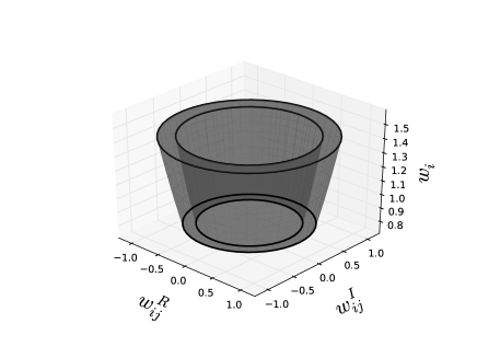
(a) Non-Convex Set without PAD Constraints.

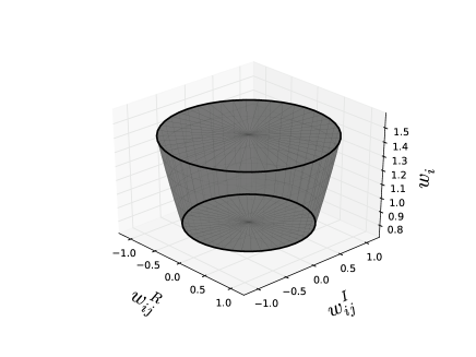
(b) Convex Hull without PAD Constraints.

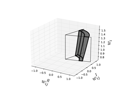
(c) Non-Convex Set with PAD Constraints

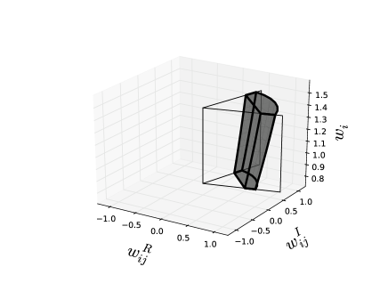
(d) Convex Hull with PAD Constraints.

Figure 1: The Implications of PAD Constraints on the Convexification of (25).

let us consider Model 5 with the parameters,

$$\bm{v^{l}}_{i}=0.9,\;\;\bm{v^{u}}_{i}=1.2,\;\;\bm{v^{l}}_{j}=0.8,\;\;\bm{v^{u}}_{j}=1.0,\;\;\bm{\theta^{l}}_{ij}=\bm{\pi}/12,\;\;\bm{\theta^{u}}_{ij}=5\bm{\pi}/12$$

Figure 1 presents the solution set of Model 5 with these parameters in the $(w^{R}_{ij},w^{I}_{ij},w_{i})$ space. This figure considers four cases, Model 5 with and without the PAD constraint (26e) and the implications that this constraint has on the convexification of (25). Figure 1(a) presents Model 5 with only constraints on the voltage variables (i.e. (26a)–(26b),(26f)) and Figure 1(b), illustrates the convex hull of that case. Figure 1(c) highlights the significant reduction in the feasible space when PAD constraints are considered (i.e. (26a)–(26f)) and Figure 1(d), illustrates the much reduced convex hull. The next subsection develops an Extreme cut representing the analytical form of the convex hull illustrated in Figure 1(d).

4.2.2 The Extreme Cut

From this point forward, we use an alternate representation of the voltage angle bounds. Specifically, given $-\bm{\pi}/2\leq\bm{\theta^{l}}_{ij}<\bm{\theta^{u}}_{ij}\leq\bm{\pi}/2$, we define the following constants:

$$\bm{\phi}_{ij}=(\bm{\theta^{u}}_{ij}+\bm{\theta^{l}}_{ij})/2$$ (28a)

$$\bm{\delta}_{ij}=(\bm{\theta^{u}}_{ij}-\bm{\theta^{l}}_{ij})/2$$ (28b)

Observe that $\bm{\theta^{l}}_{ij}=\bm{\phi}_{ij}-\bm{\delta}_{ij}$ and $\bm{\theta^{u}}_{ij}=\bm{\phi}_{ij}+\bm{\delta}_{ij}$. Additionally, we define the following constants,

$$\bm{v^{\sigma}}_{i}=\bm{v^{l}}_{i}+\bm{v^{u}}_{i}$$ (29a)

$$\bm{v^{\sigma}}_{j}=\bm{v^{l}}_{j}+\bm{v^{u}}_{j}$$ (29b)

As this section demonstrates, the $\phi,\delta,v^{\sigma}$ representation is particularly advantageous for developing concise valid inequalities for Model 5.

Theorem 4.1.

The following Extreme cut is redundant in Model 5,

$$\bm{v^{l}}_{j}\cos(\bm{\delta}_{ij})w_{i}-\bm{v^{\sigma}}_{i}\cos(\bm{\phi}_{ij})w^{R}_{ij}-\bm{v^{\sigma}}_{i}\sin(\bm{\phi}_{ij})w^{I}_{ij}+\bm{v^{l}}_{i}\bm{v^{u}}_{i}\bm{v^{l}}_{j}\cos(\bm{\delta}_{ij})\leq 0.$$ (30)

Proof.

As mentioned previously, Model 5 can be reformulated in three dimensions using equation (26f), which leads to the set

$$\mathcal{S}_{p}=\left\{\left(w^{R}_{ij},w^{I}_{ij},w_{i}\right)\in\mathbb{R}^{3}~{}\left|~{}\begin{aligned} &(\ref{eq:svfs_1}),(\ref{eq:wr_b})-(\ref{eq:svfs_3})\\ &w_{i}(\bm{v^{l}}_{j})^{2}\leq(w^{R}_{ij})^{2}+(w^{I}_{ij})^{2}\leq w_{i}(\bm{v^{u}}_{j})^{2}\end{aligned}\right.\right\}.$$

Let

$$f(w^{R}_{ij},w^{I}_{ij},w_{i})=w_{i}(\bm{v^{l}}_{j})^{2}-(w^{R}_{ij})^{2}-(w^{I}_{ij})^{2},$$

$$h(w^{R}_{ij},w^{I}_{ij},w_{i})=\bm{v^{l}}_{j}\cos(\bm{\delta}_{ij})w_{i}-\bm{v^{\sigma}}_{i}\cos(\bm{\phi}_{ij})w^{R}_{ij}-\bm{v^{\sigma}}_{i}\sin(\bm{\phi}_{ij})w^{I}_{ij}+\bm{v^{l}}_{i}\bm{v^{u}}_{i}\bm{v^{l}}_{j}\cos(\bm{\delta}_{ij}),$$

and define the set,

$$\mathcal{S}_{r}=\left\{\left(w^{R}_{ij},w^{I}_{ij},w_{i}\right)\in\mathbb{R}^{3}~{}\left|~{}\begin{aligned} &f(w^{R}_{ij},w^{I}_{ij},w_{i})\leq 0,\\ &(\bm{v^{l}}_{i})^{2}\leq w_{i}\leq(\bm{v^{u}}_{i})^{2},w^{R}_{ij}\leq\bm{v^{u}}_{i}\bm{v^{u}}_{j}\\ &\tan(\bm{\theta^{l}}_{ij})w^{R}_{ij}\leq w^{I}_{ij}\leq\tan(\bm{\theta^{u}}_{ij})w^{R}_{ij}\end{aligned}\right.\right\},$$

observe that $\mathcal{S}_{r}$ is a relaxation of $\mathcal{S}_{p}$. We will first show that $h(w^{R}_{ij},w^{I}_{ij},w_{i})\leq 0,~{}\forall(w^{R}_{ij},w^{I}_{ij},w_{i})\in\mathcal{S}_{r}$, and consequently $\forall(w^{R}_{ij},w^{I}_{ij},w_{i})\in\mathcal{S}_{p}$, as $\mathcal{S}_{p}\subset\mathcal{S}_{r}$. Consider the nonlinear program

$$\max~{}h(w^{R}_{ij},w^{I}_{ij},w_{i})$$

$$\text{ s.t. }(w^{R}_{ij},w^{I}_{ij},w_{i})\in\mathcal{S}_{r}.$$ (LPRC)

(LPRC) is a linear program with a reverse-convex constraint, or a concave budget constraint. Note that $\mathcal{S}_{r}$ is a bounded non-empty set and $f(w^{R}_{ij},w^{I}_{ij},w_{i})\leq 0$ is a non-redundant constraint as it cuts the points satisfying $w^{R}_{ij}=w^{I}_{ij}=0$. This type of problem is studied in [23, 24] where it is shown that all optimal solutions lie at the intersection of the concave constraint and the edges of the linear system (intersection of $n-1$ linear inequalities). There are only four such points in our case,

$$\mbox{point 1: }w_{i}=(\bm{v^{l}}_{i})^{2},\;\;w^{R}_{ij}=\bm{v^{l}}_{i}\bm{v^{l}}_{j}\cos(\bm{\phi}_{ij}-\bm{\delta}_{ij}),\;\;w^{I}_{ij}=\bm{v^{l}}_{i}\bm{v^{l}}_{j}\sin(\bm{\phi}_{ij}-\bm{\delta}_{ij})$$

$$\mbox{point 2: }w_{i}=(\bm{v^{l}}_{i})^{2},\;\;w^{R}_{ij}=\bm{v^{l}}_{i}\bm{v^{l}}_{j}\cos(\bm{\phi}_{ij}+\bm{\delta}_{ij}),\;\;w^{I}_{ij}=\bm{v^{l}}_{i}\bm{v^{l}}_{j}\sin(\bm{\phi}_{ij}+\bm{\delta}_{ij})$$

$$\mbox{point 3: }w_{i}=(\bm{v^{u}}_{i})^{2},\;\;w^{R}_{ij}=\bm{v^{u}}_{i}\bm{v^{l}}_{j}\cos(\bm{\phi}_{ij}-\bm{\delta}_{ij}),\;\;w^{I}_{ij}=\bm{v^{u}}_{i}\bm{v^{l}}_{j}\sin(\bm{\phi}_{ij}-\bm{\delta}_{ij})$$

$$\mbox{point 4: }w_{i}=(\bm{v^{u}}_{i})^{2},\;\;w^{R}_{ij}=\bm{v^{u}}_{i}\bm{v^{l}}_{j}\cos(\bm{\phi}_{ij}+\bm{\delta}_{ij}),\;\;w^{I}_{ij}=\bm{v^{u}}_{i}\bm{v^{l}}_{j}\sin(\bm{\phi}_{ij}+\bm{\delta}_{ij})$$

all of which satisfy $f(w^{R}_{ij},w^{I}_{ij},w_{i})=h(w^{R}_{ij},w^{I}_{ij},w_{i})=0$. Since zero is the maximizer of (LPRC), it follows that $h(w^{R}_{ij},w^{I}_{ij},w_{i})\leq 0,~{}\forall(w^{R}_{ij},w^{I}_{ij},w_{i})\in\mathcal{S}_{r}$ and consequently $\forall(w^{R}_{ij},w^{I}_{ij},w_{i})\in\mathcal{S}_{p}$.

∎

Given the valid linear cut (30), we can define a convex relaxation of $\mathcal{S}_{p}$,

$$\mathcal{S}_{c}=\left\{(w^{R}_{ij},w^{I}_{ij},w_{i})\in\mathbb{R}^{3}~{}\left|~{}\begin{aligned} &(\ref{eq:svfs_1}),(\ref{eq:wr_b})-(\ref{eq:svfs_3}),(\ref{eq:3d_cut}),\\ &(w^{R}_{ij})^{2}+(w^{I}_{ij})^{2}\leq w_{i}(\bm{v^{u}}_{j})^{2}\end{aligned}\right.\right\}.$$

An example of $\mathcal{S}_{p}$ and $\mathcal{S}_{c}$ are presented in Figures 1(c) and 1(d) respectively.
Let us emphasize that projecting the feasible region of Model 5 into the $(w^{R}_{ij},w^{I}_{ij},w_{j})$ space can lead to a similar Extreme cut,

$$\bm{v^{l}}_{i}\cos(\bm{\delta}_{ij})w_{j}-\bm{v^{\sigma}}_{j}\cos(\bm{\phi}_{ij})w^{R}_{ij}-\bm{v^{\sigma}}_{j}\sin(\bm{\phi}_{ij})w^{I}_{ij}+\bm{v^{l}}_{j}\bm{v^{u}}_{j}\bm{v^{l}}_{i}\cos(\bm{\delta}_{ij})\leq 0.$$ (31)

4.2.3 The Convex Nonlinear Cuts

Let us emphasize that the convex relaxation of Model 5 lives in a four-dimensional space, while the Extreme cuts defined above are three-dimensional, excluding the variable $w_{j}$. In this section, we utilize the convex set $\mathcal{S}_{c}$ to develop two valid four-dimensional cuts based on lifting redundant constraints in the $(w^{R}_{ij},w^{I}_{ij},w_{i})\in\mathbb{R}^{3}$ space.

The VUB Nonlinear Cut

For clarity we begin by defining the following constants,

$$\bm{c}_{11}=\bm{v^{\sigma}}_{i}\bm{v^{\sigma}}_{j}\cos(\bm{\phi}_{ij})$$ (32a)

$$\bm{c}_{12}=\bm{v^{\sigma}}_{i}\bm{v^{\sigma}}_{j}\sin(\bm{\phi}_{ij})$$ (32b)

$$\bm{c}_{13}=-\bm{v^{u}}_{j}\cos(\bm{\delta}_{ij})\bm{v^{\sigma}}_{j}$$ (32c)

$$\bm{c}_{14}=-\bm{v^{u}}_{i}\cos(\bm{\delta}_{ij})\bm{v^{\sigma}}_{i}$$ (32d)

$$\bm{c}_{15}=-\bm{v^{u}}_{i}\bm{v^{u}}_{j}\cos(\bm{\delta}_{ij})(\bm{v^{l}}_{i}\bm{v^{l}}_{j}-\bm{v^{u}}_{i}\bm{v^{u}}_{j})$$ (32e)

Consider the optimization problem,

$$\min~{}g(w^{R}_{ij},w^{I}_{ij},w_{i})=\bm{c}_{11}w^{R}_{ij}+\bm{c}_{12}w^{I}_{ij}+\bm{c}_{13}w_{i}+\bm{c}_{14}\frac{(w^{R}_{ij})^{2}+(w^{I}_{ij})^{2}}{w_{i}}+\bm{c}_{15}$$

$$\text{s.t. }\left\{\begin{aligned} &(\bm{v^{l}}_{i})^{2}\leq w_{i}\leq(\bm{v^{u}}_{i})^{2},\\ &\tan(\bm{\theta^{l}}_{ij})w^{R}_{ij}\leq w^{I}_{ij}\leq\tan(\bm{\theta^{u}}_{ij})w^{R}_{ij},\\ &\bm{v^{l}}_{j}\cos(\bm{\delta}_{ij})w_{i}-\bm{v^{\sigma}}_{i}\cos(\bm{\phi}_{ij})w^{R}_{ij}-\bm{v^{\sigma}}_{i}\sin(\bm{\phi}_{ij})w^{I}_{ij}+\bm{v^{l}}_{i}\bm{v^{u}}_{i}\bm{v^{l}}_{j}\cos(\bm{\delta}_{ij})\leq 0\end{aligned}\right.$$ (NLP)

Proposition 4.2.

The optimal objective for (NLP) is non-negative.

Proof.

In [21], Hijazi et al. prove that the function $f(x,y,z)=(x^{2}+y^{2})/z,z>0$, is convex, thus (NLP) is a concave program as $\bm{c}_{14}<0$. Based on [4], optimal solutions in (NLP) are extreme points of the feasibility region. There are four extreme points in (NLP),

$$\mbox{point 1: }w_{i}=(\bm{v^{l}}_{i})^{2},\;\;w^{R}_{ij}=\bm{v^{l}}_{i}\bm{v^{l}}_{j}\cos(\bm{\phi}_{ij}-\bm{\delta}_{ij}),\;\;w^{I}_{ij}=\bm{v^{l}}_{i}\bm{v^{l}}_{j}\sin(\bm{\phi}_{ij}-\bm{\delta}_{ij})$$

$$\mbox{point 2: }w_{i}=(\bm{v^{l}}_{i})^{2},\;\;w^{R}_{ij}=\bm{v^{l}}_{i}\bm{v^{l}}_{j}\cos(\bm{\phi}_{ij}+\bm{\delta}_{ij}),\;\;w^{I}_{ij}=\bm{v^{l}}_{i}\bm{v^{l}}_{j}\sin(\bm{\phi}_{ij}+\bm{\delta}_{ij})$$

$$\mbox{point 3: }w_{i}=(\bm{v^{u}}_{i})^{2},\;\;w^{R}_{ij}=\bm{v^{u}}_{i}\bm{v^{l}}_{j}\cos(\bm{\phi}_{ij}-\bm{\delta}_{ij}),\;\;w^{I}_{ij}=\bm{v^{u}}_{i}\bm{v^{l}}_{j}\sin(\bm{\phi}_{ij}-\bm{\delta}_{ij})$$

$$\mbox{point 4: }w_{i}=(\bm{v^{u}}_{i})^{2},\;\;w^{R}_{ij}=\bm{v^{u}}_{i}\bm{v^{l}}_{j}\cos(\bm{\phi}_{ij}+\bm{\delta}_{ij}),\;\;w^{I}_{ij}=\bm{v^{u}}_{i}\bm{v^{l}}_{j}\sin(\bm{\phi}_{ij}+\bm{\delta}_{ij})$$

all of which satisfy $g(w^{R}_{ij},w^{I}_{ij},w_{i})\geq 0$. ∎

Theorem 4.3.

In the $(w^{R}_{ij},w^{I}_{ij},w_{i})$ space, the following nonlinear cut is redundant with respect to $\mathcal{S}_{p}$.

$$\bm{c}_{11}w^{R}_{ij}+\bm{c}_{12}w^{I}_{ij}+\bm{c}_{13}w_{i}+\bm{c}_{14}\frac{(w^{R}_{ij})^{2}+(w^{I}_{ij})^{2}}{w_{i}}+\bm{c}_{15}\geq 0$$ (33a)

Proof.

Since the feasibility space of (NLP) is a relaxation of $\mathcal{S}_{c}$, Proposition 4.2 implies that

$$g(w^{R}_{ij},w^{I}_{ij},w_{i})\geq 0,\forall(w^{R}_{ij},w^{I}_{ij},w_{i})\in\mathcal{S}_{c},$$

thus constraint (33a) is redundant for $\mathcal{S}_{c}$ and consequently for the restricted set $\mathcal{S}_{p}$. ∎

The VLB Nonlinear Cut

For clarity we begin by defining the following constants,

$$\bm{c}_{21}=\bm{v^{\sigma}}_{i}\bm{v^{\sigma}}_{j}\cos(\bm{\phi}_{ij})$$

$$\bm{c}_{22}=\bm{v^{\sigma}}_{i}\bm{v^{\sigma}}_{j}\sin(\bm{\phi}_{ij})$$

$$\bm{c}_{23}=-\bm{v^{l}}_{j}\cos(\bm{\delta}_{ij})\bm{v^{\sigma}}_{j}$$

$$\bm{c}_{24}=-\bm{v^{l}}_{i}\cos(\bm{\delta}_{ij})\bm{v^{\sigma}}_{i}$$

$$\bm{c}_{25}=\bm{v^{l}}_{i}\bm{v^{l}}_{j}\cos(\bm{\delta}_{ij})(\bm{v^{l}}_{i}\bm{v^{l}}_{j}-\bm{v^{u}}_{i}\bm{v^{u}}_{j})$$

Theorem 4.4.

In the $(w^{R}_{ij},w^{I}_{ij},w_{i})$ space, the following nonlinear cut is redundant with respect to $\mathcal{S}_{p}$.

$$\bm{c}_{21}w^{R}_{ij}+\bm{c}_{22}w^{I}_{ij}+\bm{c}_{23}w_{i}+\bm{c}_{24}\frac{(w^{R}_{ij})^{2}+(w^{I}_{ij})^{2}}{w_{i}}+\bm{c}_{25}\geq 0$$ (35a)

Proof.

The proof of Theorem 4.3 can be adapted to fit the new parameters introduced here.

∎

Corollary 4.5.

Constraints (33a) and (35a) are valid nonlinear inequalities in any power flow model or power flow relaxation.

4.2.4 Application of the Valid Inequalities

The usefulness of the nonlinear cuts (33a) and (35a) is not immediately clear. Indeed, the Extreme cut (30) appears to provide the tightest convex relaxation of the three-dimensional non-convex set defined in Model 5. However, it is important to point out that as soon as we relax the quadratic equation (26f), we lift the feasible region into four dimensions, that is $(w^{R}_{ij},w^{I}_{ij},w_{i},w_{j})\in\mathbb{R}^{4}$. The key insight is that although (33a) and (35a) are redundant in the three-dimensional space, they are not redundant in the lifted $\mathbb{R}^{4}$ space. This property was observed in [37], where a collection of line flow constraints, which are equivalent in the non-convex space, were shown to have different strengths in the lifted convex relaxation space. Utilizing the equivalence $((w^{R}_{ij})^{2}+(w^{I}_{ij})^{2})/w_{i}=w_{j}$, we can lift (33a) and (35a) into the standard $\mathbb{R}^{4}$ power flow relaxation space as follows,

$$\bm{v^{\sigma}}_{i}\bm{v^{\sigma}}_{j}(w^{R}_{ij}\cos(\bm{\phi}_{ij})+w^{I}_{ij}\sin(\bm{\phi}_{ij}))-\bm{v^{u}}_{j}\cos(\bm{\delta}_{ij})\bm{v^{\sigma}}_{j}w_{i}-\bm{v^{u}}_{i}\cos(\bm{\delta}_{ij})\bm{v^{\sigma}}_{i}w_{j}\geq\bm{v^{u}}_{i}\bm{v^{u}}_{j}\cos(\bm{\delta}_{ij})(\bm{v^{l}}_{i}\bm{v^{l}}_{j}-\bm{v^{u}}_{i}\bm{v^{u}}_{j})$$ (36a)

$$\bm{v^{\sigma}}_{i}\bm{v^{\sigma}}_{j}(w^{R}_{ij}\cos(\bm{\phi}_{ij})+w^{I}_{ij}\sin(\bm{\phi}_{ij}))-\bm{v^{l}}_{j}\cos(\bm{\delta}_{ij})\bm{v^{\sigma}}_{j}w_{i}-\bm{v^{l}}_{i}\cos(\bm{\delta}_{ij})\bm{v^{\sigma}}_{i}w_{j}\geq-\bm{v^{l}}_{i}\bm{v^{l}}_{j}\cos(\bm{\delta}_{ij})(\bm{v^{l}}_{i}\bm{v^{l}}_{j}-\bm{v^{u}}_{i}\bm{v^{u}}_{j})$$ (36b)

We refer to these constraints as lifted nonlinear cuts (LNC). Noting that these constraints are linear in the $\mathbb{R}^{4}$ space, they can be easily integrated into any of the models discussed in Section 3.

Proposition 4.6.

The LNC cuts dominate the Extreme cuts in the $(w^{R}_{ij},w^{I}_{ij},w_{i},w_{j})$ space.

Proof.

Observe that replacing $w_{j}$ (resp. $w_{i}$) by its lower bound in (36b) (resp. (36a)) leads to (30) (resp. (31)). Given that the coefficients corresponding to $w_{i}$ and $w_{j}$ are both negative in (36a) and (36b), dominance is guaranteed. ∎

4.2.5 Connections to Previous Work

To the best of our knowledge, two previous work in the power systems community [37, 29] have explored similar ideas for strengthening the SDP relaxation. Two interesting observations were made in [37]: (1) when the voltage magnitudes at both sides of the line are fixed, the maximum phase difference $\bm{\theta^{m}}_{ij}$ can be used to encode a variety of equivalent line capacity constraints; (2) from these equivalent flow limit constraints, the current limit constraint was observed to be the most advantageous for the SDP relaxation. Specifically, in the notation of this paper, [37] concludes that for the intervals $w_{i}=1,w_{j}=1,\bm{\theta^{l}}_{ij}=-\bm{\theta^{m}}_{ij},\bm{\theta^{u}}_{ij}=\bm{\theta^{m}}_{ij}$, the strongest line flow constraint in the SDP relaxation is $w_{i}+w_{j}-2w^{R}_{ij}\leq 2(1-\cos(\bm{\theta^{m}}_{ij}))$. Knowing that the values of $w_{i},w_{j}$ are fixed, this constraint reduces to:

$$w^{R}_{ij}\geq\cos(\bm{\theta^{m}}_{ij})$$ (37)

Now let us apply the same special case to the lifted nonlinear cuts developed here. The constants for this special case are $\bm{\phi}_{ij}=0;\;\bm{\delta}_{ij}=\bm{\theta^{m}}_{ij};\;\bm{v^{\sigma}}_{i},\bm{v^{\sigma}}_{j}=2;\;\bm{v^{l}}_{i},\bm{v^{u}}_{i},\bm{v^{l}}_{j},\bm{v^{u}}_{i}=1$ and the application to (36a) is as follows:

$$\bm{v^{\sigma}}_{i}\bm{v^{\sigma}}_{j}(w^{R}_{ij}\cos(\bm{\phi}_{ij})+w^{I}_{ij}\sin(\bm{\phi}_{ij}))-\bm{v^{u}}_{j}\cos(\bm{\delta}_{ij})\bm{v^{\sigma}}_{j}w_{i}-\bm{v^{u}}_{i}\cos(\bm{\delta}_{ij})\bm{v^{\sigma}}_{i}w_{j} \geq\bm{v^{u}}_{i}\bm{v^{u}}_{j}\cos(\bm{\delta}_{ij})(\bm{v^{l}}_{i}\bm{v^{l}}_{j}-\bm{v^{u}}_{i}\bm{v^{u}}_{j})$$ (38a)

$$4w^{R}_{ij}-\cos(\bm{\theta^{m}}_{ij})2w_{i}-\cos(\bm{\theta^{m}}_{ij})2w_{j} \geq 0$$ (38b)

$$2w^{R}_{ij}-\cos(\bm{\theta^{m}}_{ij})(w_{i}+w_{j}) \geq 0$$ (38c)

$$w^{R}_{ij} \geq\cos(\bm{\theta^{m}}_{ij})$$ (38d)

This reduction shows that the lifted nonlinear cuts proposed here are a generalization dominating the current limit constraint proposed in [37].

In an entirely different approach, valid cuts based on the bounds of $w^{R}$ and $w^{I}$ were proposed in [29]. These cuts have a key advantage over the line limit constraints considered in [37] in that they can capture the structure of asymmetrical bounds on $\bm{\theta^{l}},\bm{\theta^{u}}$. For example, consider the case where $0\leq\bm{\theta^{l}}_{ij}<\bm{\theta^{u}}_{ij}\leq\bm{\pi}/2$. In this case, [29] proposes the following cut,

$$w^{R}_{ij}\cos(\bm{\phi}_{ij})+w^{I}_{ij}\sin(\bm{\phi}_{ij})\geq\bm{v^{l}}_{i}\bm{v^{l}}_{j}\cos(\bm{\delta}_{ij})$$ (39a)

A derivation of this cut from the algorithm provided in [29] can be found in Appendix B.

Proposition 4.7.

The new nonlinear lifted cuts (36b) dominate constraints (39a).

Proof.

To support the proof, we first observe the following property,

$$\bm{v^{l}}_{j}\bm{v^{\sigma}}_{j}(\bm{v^{l}}_{i})^{2}+\bm{v^{l}}_{i}\bm{v^{\sigma}}_{i}(\bm{v^{l}}_{j})^{2}-\bm{v^{l}}_{i}\bm{v^{l}}_{j}(\bm{v^{l}}_{i}\bm{v^{l}}_{j}-\bm{v^{u}}_{i}\bm{v^{u}}_{j})=$$ (40a)

$$(\bm{v^{l}}_{j})^{2}(\bm{v^{l}}_{i})^{2}+\bm{v^{l}}_{j}\bm{v^{u}}_{j}(\bm{v^{l}}_{i})^{2}+(\bm{v^{l}}_{i})^{2}(\bm{v^{l}}_{j})^{2}+\bm{v^{l}}_{i}\bm{v^{u}}_{i}(\bm{v^{l}}_{j})^{2}-(\bm{v^{l}}_{i}\bm{v^{l}}_{j})^{2}+\bm{v^{l}}_{i}\bm{v^{l}}_{j}\bm{v^{u}}_{i}\bm{v^{u}}_{j}=$$ (40b)

$$(\bm{v^{l}}_{i}\bm{v^{l}}_{j}+\bm{v^{l}}_{i}\bm{v^{u}}_{j}+\bm{v^{u}}_{i}\bm{v^{l}}_{j}+\bm{v^{u}}_{i}\bm{v^{u}}_{j})\bm{v^{l}}_{i}\bm{v^{l}}_{j}=$$ (40c)

$$(\bm{v^{l}}_{i}+\bm{v^{u}}_{i})(\bm{v^{l}}_{j}+\bm{v^{u}}_{j})\bm{v^{l}}_{i}\bm{v^{l}}_{j}=$$ (40d)

$$\bm{v^{\sigma}}_{i}\bm{v^{\sigma}}_{j}\bm{v^{l}}_{i}\bm{v^{l}}_{j}$$ (40e)

Now assume $w_{i}=(\bm{v^{l}}_{i})^{2},w_{j}=(\bm{v^{l}}_{j})^{2}$ and apply (36b) as follows,

$$\bm{v^{\sigma}}_{i}\bm{v^{\sigma}}_{j}(w^{R}_{ij}\cos(\bm{\phi}_{ij})+w^{I}_{ij}\sin(\bm{\phi}_{ij}))-\bm{v^{l}}_{j}\cos(\bm{\delta}_{ij})\bm{v^{\sigma}}_{j}w_{i}-\bm{v^{l}}_{i}\cos(\bm{\delta}_{ij})\bm{v^{\sigma}}_{i}w_{j} \geq-\bm{v^{l}}_{i}\bm{v^{l}}_{j}\cos(\bm{\delta}_{ij})(\bm{v^{l}}_{i}\bm{v^{l}}_{j}-\bm{v^{u}}_{i}\bm{v^{u}}_{j})$$ (41a)

$$\bm{v^{\sigma}}_{i}\bm{v^{\sigma}}_{j}(w^{R}_{ij}\cos(\bm{\phi}_{ij})+w^{I}_{ij}\sin(\bm{\phi}_{ij}))-\bm{v^{l}}_{j}\cos(\bm{\delta}_{ij})\bm{v^{\sigma}}_{j}(\bm{v^{l}}_{i})^{2}-\bm{v^{l}}_{i}\cos(\bm{\delta}_{ij})\bm{v^{\sigma}}_{i}(\bm{v^{l}}_{j})^{2} \geq-\bm{v^{l}}_{i}\bm{v^{l}}_{j}\cos(\bm{\delta}_{ij})(\bm{v^{l}}_{i}\bm{v^{l}}_{j}-\bm{v^{u}}_{i}\bm{v^{u}}_{j})$$ (41b)

$$\bm{v^{\sigma}}_{i}\bm{v^{\sigma}}_{j}(w^{R}_{ij}\cos(\bm{\phi}_{ij})+w^{I}_{ij}\sin(\bm{\phi}_{ij})) \geq\bm{v^{\sigma}}_{i}\bm{v^{\sigma}}_{j}\bm{v^{l}}_{i}\bm{v^{l}}_{j}\cos(\bm{\delta}_{ij})$$ (41c)

$$w^{R}_{ij}\cos(\bm{\phi}_{ij})+w^{I}_{ij}\sin(\bm{\phi}_{ij}) \geq\bm{v^{l}}_{i}\bm{v^{l}}_{j}\cos(\bm{\delta}_{ij})$$ (41d)

A similar analysis can be done to confirm that (39a) is a weaker version of the extreme cut (30). It is now clear that the cut proposed in [29] is a special case of the cuts proposed here, where the voltage variables are assigned to their lower bounds. ∎

In a very recent and independent line of work, coming out of the mathematical programming community, [10] considers a model similar to Model 5. The key difference being in the parameterization the variable bounds and the coefficients of (26e). Using a representation where $\tan(\bm{\theta^{l}}_{ij})=\bm{t^{l}}_{ij},\tan(\bm{\theta^{u}}_{ij})=\bm{t^{u}}_{ij},(\bm{v^{l}}_{i})^{2}=\bm{w^{l}}_{i}$, and so on, [10] proposes the following constants,

$$\bm{\pi}_{0}=-\sqrt{\bm{w^{l}}_{i}\bm{w^{l}}_{j}\bm{w^{u}}_{i}\bm{w^{u}}_{j}}$$ (42a)

$$\bm{\pi}_{1}=-\sqrt{\bm{w^{l}}_{j}\bm{w^{u}}_{j}}$$ (42b)

$$\bm{\pi}_{2}=-\sqrt{\bm{w^{l}}_{i}\bm{w^{u}}_{i}}$$ (42c)

$$\bm{\pi}_{3}=\left(\sqrt{\bm{w^{l}}_{i}}+\sqrt{\bm{w^{u}}_{i}}\right)\left(\sqrt{\bm{w^{l}}_{j}}+\sqrt{\bm{w^{u}}_{j}}\right)\frac{1-\left(\frac{\sqrt{1+(\bm{t^{l}}_{ij})^{2}}-1}{\bm{t^{l}}_{ij}}\right)\left(\frac{\sqrt{1+(\bm{t^{u}}_{ij})^{2}}-1}{\bm{t^{u}}_{ij}}\right)}{1+\left(\frac{\sqrt{1+(\bm{t^{l}}_{ij})^{2}}-1}{\bm{t^{l}}_{ij}}\right)\left(\frac{\sqrt{1+(\bm{t^{u}}_{ij})^{2}}-1}{\bm{t^{u}}_{ij}}\right)}$$ (42d)

$$\bm{\pi}_{4}=\left(\sqrt{\bm{w^{l}}_{i}}+\sqrt{\bm{w^{u}}_{i}}\right)\left(\sqrt{\bm{w^{l}}_{j}}+\sqrt{\bm{w^{u}}_{j}}\right)\frac{\left(\frac{\sqrt{1+(\bm{t^{l}}_{ij})^{2}}-1}{\bm{t^{l}}_{ij}}\right)+\left(\frac{\sqrt{1+(\bm{t^{u}}_{ij})^{2}}-1}{\bm{t^{u}}_{ij}}\right)}{1+\left(\frac{\sqrt{1+(\bm{t^{l}}_{ij})^{2}}-1}{\bm{t^{l}}_{ij}}\right)\left(\frac{\sqrt{1+(\bm{t^{u}}_{ij})^{2}}-1}{\bm{t^{u}}_{ij}}\right)}$$ (42e)

and then develops the following valid inequalities,

$$\bm{\pi}_{0}+\bm{\pi}_{1}w_{i}+\bm{\pi}_{2}w_{j}+\bm{\pi}_{3}w^{R}_{ij}+\bm{\pi}_{4}w^{I}_{ij}\geq\bm{w^{u}}_{j}w_{i}+\bm{w^{u}}_{i}w_{j}-\bm{w^{u}}_{i}\bm{w^{u}}_{j}$$ (43a)

$$\bm{\pi}_{0}+\bm{\pi}_{1}w_{i}+\bm{\pi}_{2}w_{j}+\bm{\pi}_{3}w^{R}_{ij}+\bm{\pi}_{4}w^{I}_{ij}\geq\bm{w^{l}}_{j}w_{i}+\bm{w^{l}}_{i}w_{j}-\bm{w^{l}}_{i}\bm{w^{l}}_{j}$$ (43b)

Proposition 4.8.

Using the parameterization of Model 5, the valid inequalities (43a),(43b) are equivalent to (36a),(36b), respectively.

A proof can be found in Appendix C.

This result highlights how the transcendental characterization of the constant values (e.g. $\cos(\bm{\phi}_{ij})$, $\cos(\bm{\delta}_{ij})$, $\tan(\bm{\theta^{l}}_{ij})$, …) used in Model 5 simplifies the presentation of these valid inequalities as well as the proofs of their validity.

Together, all of these connections illustrate that the lifted nonlinear cuts proposed here and the valid inequalities from [10] are a generalization of the cuts proposed in [37] and [29] that combines the strengths of both previous works.

4.3 Bound Tightening

It was observed in [15] that both the SDP and QC models benefit significantly from tightening the bounds on $v_{i}$ and $\theta_{ij}$. Additionally, the convex envelopes of the QC model and all of the cuts proposed here also benefit form tight bounds. Hence, we utilize the minimal network consistency algorithm proposed in [15] to strengthen all of the relaxations considered here.

4.4 Impact on Model Size

This section has introduced a variety of methods for strengthening the SDP relaxation (i.e. Model 2), including adding the QC model constraints and/or lifted nonlinear cuts. It is important to take note of the model size implications of each of these approaches. The lifted nonlinear cuts are a notably light-weight improvement to the SDP relaxation and only require adding $2|E|$ linear constraints, and no additional variables. The QC constraints increase the model’s size significantly and require adding $2|V|+5|E|$ variables, $1+|V|+15|E|$ linear constraints, and $|V|+|E|$ quadratic constraints. Consequently, one would expect the QC model to be stronger than the lifted nonlinear cuts but at the cost of a significant computation burden.

5 Experimental Evaluation

This section assesses the benefits of all three SDP strengthening approaches in a step-wise fashion. The assessment is done by comparing four variants of the SDP relaxation for bounding primal AC-OPF solutions produced by IPOPT, which only guarantees local optimality. The four relaxations under consideration are as follows:

1. SDP-N : the SDP relaxation strengthened with the bound tightening proposed in [15].

2. SDP-N+LNC : SDP-N with the addition of lifted nonlinear cuts.

3. SDP-N+QC : SDP-N with the conjunction of the QC model.

4. SDP-N+QC+LNC : SDP-N with the QC model and lifted nonlinear cuts.

Experimental Setting

All of the computations are conducted on Dell PowerEdge R415 servers with Dual 3.1GHz AMD 6-Core Opteron 4334 CPUs and 64GB of memory. IPOPT 3.12 [56] with linear solver ma27 [53], as suggested by [8], was used as a heuristic for finding locally optimal feasible solutions to the non-convex AC-OPF formulated in AMPL [17]. The SDP relaxations were based on the state-of-the-art implementation [31] which uses a branch decomposition [35] for performance and scalability gains. The SDP solver SDPT3 4.0 [51] was used with the modifications suggested in [31]. The tight variable bounds for SDP-N are pre-computed using the algorithm in [15]. If all of the subproblems are computed in parallel, the bound tightening computation adds an overhead of less than 1 minute, which is not reflected in the runtime results presented here.

Open Test Cases

Due to the computational burden of using modern SDP solvers on cases with more than 1000-buses [14], the evaluation was conducted on 71 test cases from NESTA v0.6.0 [11] that have less than 1000-buses. Among these 71 test cases it was observed that the base case, SDP-N, was able to close the optimality gap to less than 1.0% in 55 cases, leaving 16 open test cases. Hence, we focus our attention on those test cases where the SDP-N optimality gap is greater than 1.0%. Detailed performance and runtime results are present in Table 1 and can be summarized as follows:

1. SDP-N+LNC brings significant improvements to the SDP-N relaxation, often reducing the optimality gap by several percentage points.

2. SDP-N+QC is generally stronger than SDP-N+LNC, however nesta_case162_ieee_dtc__sad,
   nesta_case9_na_cao__nco, nesta_case9_nb_cao__nco are notable exceptions, illustrating that there is value in adding both the QC model and the lifted nonlinear cuts to the SDP relaxation.

3. The strongest model, SDP-N+QC+LNC, has reduced to optimality gap of 8 of the 16 of the open cases to less than 1% (i.e. closing 50% of the open cases), leaving only 8 for further investigation. Furthermore, on 3 of the 8 open cases, the AC solution is known to be globally optimal, indicating that the only source of the optimality gap comes from convexificaiton. These cases are ideal candidates for evaluation of nonconvex optimization algorithms.

4. Although the size of the SDP-N+QC model is significantly larger than SDP-N+LNC (as discussed in Section 4.4), we observe that the runtimes do not vary significantly. We suspect that the SDP iteration computation dominates the runtime on the test cases considered here.

Table 1: Quality and Runtime Results of AC Power Flow Relaxations (open cases)

	$/h	Optimality Gap (%)				Runtime (seconds)
					+QC					+QC
Test Case	AC	SDP-N	+LNC	+QC	+LNC	AC	SDP-N	+LNC	+QC	+LNC
Typical Operating Conditions (TYP)
nesta_case5_pjm	17551.89	5.22	5.06	3.96	3.96	0.16	3.18	2.92	3.36	3.04
Congested Operating Conditions (API)
nesta_case30_fsr__api	372.14	3.58	1.03	0.89	0.61	0.09	3.63	5.38	5.46	5.56
nesta_case89_pegase__api	4288.02	18.11	18.08⋆	17.09⋆	16.60⋆	0.50	12.44	13.17	47.50	28.27
nesta_case118_ieee__api	10325.27	16.72	8.70	3.40	3.32	0.40	8.49	9.61	10.73	13.62
Small Angle Difference Conditions (SAD)
nesta_case24_ieee_rts__sad	79804.30	1.38	0.05	0.07	0.02	0.20	3.80	4.13	3.27	3.77
nesta_case29_edin__sad	46931.74	5.79	1.90	0.53	0.50	0.35	4.70	5.34	6.23	6.11
nesta_case73_ieee_rts__sad	235241.58	2.41	0.18	0.05	0.03	0.26	6.44	6.80	8.01	8.51
nesta_case118_ieee__sad	4324.17	4.04	1.16	0.83	0.74	0.32	11.21	10.44	11.65	14.31
nesta_case162_ieee_dtc__sad	4369.19	1.73	0.37	1.49	0.35	0.68	20.16	20.18	53.54	40.58
nesta_case189_edin__sad	914.64	1.20⋆	0.89⋆	err.	0.86⋆	0.29	7.51	10.91	36.24⋆	54.44
Nonconvex Optimization Cases (NCO)
nesta_case9_na_cao__nco	-212.43	18.00	11.66	15.91	11.62	0.05	2.42	2.66	3.26	2.30
nesta_case9_nb_cao__nco	-247.42	19.23	11.77	16.46	11.76	0.18	2.44	2.55	2.06	2.31
nesta_case14_s_cao__nco	9670.44	2.96	2.92	2.06	2.03	0.07	3.21	2.86	2.91	3.10
Radial Toplogies (RAD)
nesta_case9_kds__rad	11279.48	1.09	0.13	1.04⋆	0.13	0.29	2.47	2.34	2.08	2.54
nesta_case30_kds__rad	4336.18†	2.11	1.88	1.97	1.88	n.a.	4.02	3.25	6.51	3.84
nesta_case30_l_kds__rad	3607.73†	15.86	15.56	15.76	15.56	n.a.	3.53	3.28	4.69	4.26

bold - known global optimum, $\dagger$ - best known solution (not initial ipopt solution), $\star$ - solver reported numerical accuracy warnings.

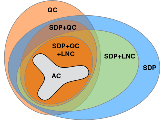
Figure 2: A Venn Diagram of the Solutions Sets for Various SDP Relaxations (set sizes in this illustration are not to scale).

Relations of the Power Flow Relaxations

From the results presented in Table 1, we can conclude that the QC and lifted nonlinear cuts have different strengths and weaknesses and one does not dominate the other. Using this information, Figure 2 presents an updated Venn Diagram of relaxations (originally presented in [14]) to reflect the various strengthened relaxations considered here.

6 Conclusion

With several years of steady progress on convex relaxations of the AC power flow equations, the optimality gap on the vast majority of AC Optimal Power Flow (AC-OPF) test cases has been closed to less than 1%. This paper sought to push the limits of convex relaxations even further and close the optimality gap on the 16 remaining open test cases. To that end, the SDP-N+QC+LNC power flow relaxation was developed by hybridizing the SDP and QC relaxations, proposing lifted nonlinear cuts, and performing bounds propagation. The proposed model was able to reduce the optimality gap to less than 1% on 8 of the 16 open cases. Overall, this approach was able to close the gap on 88.7% of the 71 AC-OPF cases considered herein.

The key weakness of the SDP-N+QC+LNC relaxation is its reliance on SDP solving technology, which suffers from scalability limitations [14]. Fortunately, recent works have proposed promising approaches for scaling the SDP relaxations to larger test cases [22, 28]. Despite the current scalability challenges, it may still be beneficial to perform this costly SDP computation at the root node of a branch-and-bound method for proving a tight lower bound. Indeed, after ten hours of computation, off-the-shelf global optimization solvers [1, 3] cannot close the optimality gap on the vast majority of AC-OPF test cases.

Thinking more broadly, this work highlights two notable facts about the classic AC-OPF problem. First, interior point methods (e.g., Ipopt) are able to find globally optimal solutions in the vast majority of test cases. Second, it is possible to enclose the non-convex AC-OPF feasibility region in tight convex set, leading to convex relaxations providing very small optimality gaps. Both of these results are interesting given that the AC-OPF is a non-convex optimization problem, which is known to be NP-Hard in general [55, 33].

Appendix A Analysis of Extreme Values of $W_{ij}$

This appendix analyzes the extreme points of $W_{ij}$ in the nonconvex Model 1 to develop valid variable bounds for $W_{ij}$. We begin by developing some basic properties about the minimum and maximum values of various functions. Then we will compose these properties to develop valid bounds for $W_{ij}$.

Let $f(x,y)=xy$. First we consider the case of multiplying two positive numbers, namely,

$$0\leq\bm{x^{l}}\leq\bm{x^{u}},0\leq\bm{y^{l}}\leq\bm{y^{u}}$$ (44a)

observe that the values of $f(x,y)$ are ordered as follows,

$$f(\bm{x^{l}},\bm{y^{l}})\leq f(\bm{x^{u}},\bm{y^{l}}),f(\bm{x^{l}},\bm{y^{u}})\leq f(\bm{x^{u}},\bm{y^{u}})$$ (45a)

consequently we have,

Lemma A.1.

For positive $x$ and $y$,

$$\min(xy) =\bm{x^{l}}\bm{y^{l}}$$ (46a)

$$\max(xy) =\bm{x^{u}}\bm{y^{u}}$$ (46b)

Second we consider the case of multiplying a positive number with a negative number, namely,

$$0\leq\bm{x^{l}}\leq\bm{x^{u}},\bm{y^{l}}\leq\bm{y^{u}}\leq 0$$ (47a)

observe that the values of $f(x,y)$ are ordered as follows,

$$f(\bm{x^{u}},\bm{y^{l}})\leq f(\bm{x^{l}},\bm{y^{l}}),f(\bm{x^{u}},\bm{y^{u}})\leq f(\bm{x^{l}},\bm{y^{u}})$$ (48a)

consequently we have,

Lemma A.2.

For positive $x$ and negative $y$,

$$\min(xy) =\bm{x^{u}}\bm{y^{l}}$$ (49a)

$$\max(xy) =\bm{x^{l}}\bm{y^{u}}$$ (49b)

Third we consider the case of multiplying a positive number with a negative or positive number, namely,

$$0\leq\bm{x^{l}}\leq\bm{x^{u}},\bm{y^{l}}\leq 0\leq\bm{y^{u}}$$ (50a)

observe that the values of $f(x,y)$ are ordered as follows,

$$f(\bm{x^{u}},\bm{y^{l}})\leq f(\bm{x^{l}},\bm{y^{l}})\leq f(\bm{x^{l}},\bm{y^{u}})\leq f(\bm{x^{u}},\bm{y^{u}})$$ (51a)

consequently we have,

Lemma A.3.

For positive $x$ and positive or negative $y$,

$$\min(xy) =\bm{x^{u}}\bm{y^{l}}$$ (52a)

$$\max(xy) =\bm{x^{u}}\bm{y^{u}}$$ (52b)

Next we consider the extreme values of $f(x)=\sin(x)$ and $g(x)=\cos(x)$ on the interval $-\bm{\pi}/2\leq x\leq\bm{\pi}/2$. Observing that $\cos(x)$ is non-monotone and has an inflection point at $x=0$, we will break this into three cases based on if the range includes the inflection point, specifically, $-\bm{\pi}/2\leq\bm{x^{l}}\leq\bm{x^{u}}\leq 0$, $-\bm{\pi}/2\leq\bm{x^{l}}<0<\bm{x^{u}}\leq\bm{\pi}/2$, and $0\leq\bm{x^{l}}\leq\bm{x^{u}}\leq\bm{\pi}/2$. For the first interval $\cos(x)$ is monotone increasing, thus,

Lemma A.4.

For $-\bm{\pi}/2\leq\bm{x^{l}}\leq\bm{x^{u}}\leq 0$,

$$\min(\cos(x)) =\cos(\bm{x^{l}})$$ (53a)

$$\max(\cos(x)) =\cos(\bm{x^{u}})$$ (53b)

For the second interval $\cos(x)$ passes through the inflection point and this is the maximum value at $x=0$. The minimum value can occur on either side (i.e. $x<0$ or $x>0$) depending interval, however because both sides are monotone we know the minimum value will occur at one of the extreme points.

Lemma A.5.

For $-\bm{\pi}/2\leq\bm{x^{l}}<0<\bm{x^{u}}\leq\bm{\pi}/2$,

$$\min(\cos(x)) =\min(\cos(\bm{x^{l}}),\cos(\bm{x^{u}}))$$ (54a)

$$\max(\cos(x)) =\cos(0)=1$$ (54b)

For the third interval $\cos(x)$ is monotone decreasing, thus,

Lemma A.6.

For $0\leq\bm{x^{l}}\leq\bm{x^{u}}\leq\bm{\pi}/2$,

$$\min(\cos(x)) =\cos(\bm{x^{u}})$$ (55a)

$$\max(\cos(x)) =\cos(\bm{x^{l}})$$ (55b)

Given that $\sin(x)$ is monotone increasing over the complete range of $x$ only one case is nessiary,

Lemma A.7.

For $-\bm{\pi}/2\leq x\leq\bm{\pi}/2$,

$$\min(\sin(x)) =\sin(\bm{x^{l}})$$ (56a)

$$\max(\sin(x)) =\sin(\bm{x^{u}})$$ (56b)

However, it is important to note that $\sin(x)$ is negative for $x<0$ and positive for $x\geq 0$. This is the only function considered thus far, which can yield negative values.

With these basic properties defined we are now in a position to develop bounds on $W_{ij}$. We begin by noting the following real valued interpretation of $W_{ij}$,

$$\Re(W_{ij})=w^{R}_{ij}=v_{i}v_{j}\cos(\theta)$$ (57a)

$$\Im(W_{ij})=w^{I}_{ij}=v_{i}v_{j}\sin(\theta)$$ (57b)

and the variable bounds from Model 1,

$$\bm{v^{l}}_{i} \leq v_{i}\leq\bm{v^{u}}_{i}$$ (58a)

$$\bm{v^{l}}_{j} \leq v_{j}\leq\bm{v^{u}}_{j}$$ (58b)

$$-\bm{\pi}/2\leq\bm{\theta^{l}}_{ij} \leq\theta_{ij}\leq\bm{\theta^{u}}_{ij}\leq\bm{\pi}/2$$ (58c)

Next we can compute values for $\min,\max$ of $w^{R}_{ij},w^{I}_{ij}$ by composing the properties developed previously. The analysis is broken into three cases based on the bounds of $\theta_{ij}$, to account for the inflection point in the cosine function.

Case 1

In the range $-\bm{\pi}/2\leq\bm{x^{l}}\leq\bm{x^{u}}\leq 0$,

$\min(w^{R}_{ij})$	$\max(w^{R}_{ij})$	$\min(w^{I}_{ij})$	$\max(w^{I}_{ij})$
$\min(v_{i}v_{j}\cos(\theta))$	$\max(v_{i}v_{j}\cos(\theta))$	$\min(v_{i}v_{j}\sin(\theta))$	$\max(v_{i}v_{j}\sin(\theta))$
$\min(v_{i}v_{j})\min(\cos(\theta))$	$\max(v_{i}v_{j})\max(\cos(\theta))$	$\max(v_{i}v_{j})\min(\sin(\theta))$	$\min(v_{i}v_{j})\max(\sin(\theta))$
$\bm{v^{l}}_{i}\bm{v^{l}}_{j}\cos(\bm{\theta^{l}}_{ij})$	$\bm{v^{u}}_{i}\bm{v^{u}}_{j}\cos(\bm{\theta^{u}}_{ij})$	$\bm{v^{u}}_{i}\bm{v^{u}}_{j}\sin(\bm{\theta^{l}}_{ij})$	$\bm{v^{l}}_{i}\bm{v^{l}}_{j}\sin(\bm{\theta^{u}}_{ij})$

Case 2

In the range $-\bm{\pi}/2\leq\bm{x^{l}}<0<\bm{x^{u}}\leq\bm{\pi}/2$,

$\min(w^{R}_{ij})$	$\max(w^{R}_{ij})$	$\min(w^{I}_{ij})$	$\max(w^{I}_{ij})$
$\min(v_{i}v_{j}\cos(\theta))$	$\max(v_{i}v_{j}\cos(\theta))$	$\min(v_{i}v_{j}\sin(\theta))$	$\max(v_{i}v_{j}\sin(\theta))$
$\min(v_{i}v_{j})\min(\cos(\theta))$	$\max(v_{i}v_{j})\max(\cos(\theta))$	$\max(v_{i}v_{j})\min(\sin(\theta))$	$\max(v_{i}v_{j})\max(\sin(\theta))$
$\bm{v^{l}}_{i}\bm{v^{l}}_{j}\min(\cos(\bm{\theta^{l}}_{ij}),\cos(\bm{\theta^{u}}_{ij}))$	$\bm{v^{u}}_{i}\bm{v^{u}}_{j}$	$\bm{v^{u}}_{i}\bm{v^{u}}_{j}\sin(\bm{\theta^{l}}_{ij})$	$\bm{v^{u}}_{i}\bm{v^{u}}_{j}\sin(\bm{\theta^{u}}_{ij})$

Case 3

In the range $0\leq\bm{x^{l}}\leq\bm{x^{u}}\leq\bm{\pi}/2$,

$\min(w^{R}_{ij})$	$\max(w^{R}_{ij})$	$\min(w^{I}_{ij})$	$\max(w^{I}_{ij})$
$\min(v_{i}v_{j}\cos(\theta))$	$\max(v_{i}v_{j}\cos(\theta))$	$\min(v_{i}v_{j}\sin(\theta))$	$\max(v_{i}v_{j}\sin(\theta))$
$\min(v_{i}v_{j})\min(\cos(\theta))$	$\max(v_{i}v_{j})\max(\cos(\theta))$	$\min(v_{i}v_{j})\min(\sin(\theta))$	$\max(v_{i}v_{j})\max(\sin(\theta))$
$\bm{v^{l}}_{i}\bm{v^{l}}_{j}\cos(\bm{\theta^{u}}_{ij})$	$\bm{v^{u}}_{i}\bm{v^{u}}_{j}\cos(\bm{\theta^{l}}_{ij})$	$\bm{v^{l}}_{i}\bm{v^{l}}_{j}\sin(\bm{\theta^{l}}_{ij})$	$\bm{v^{u}}_{i}\bm{v^{u}}_{j}\sin(\bm{\theta^{u}}_{ij})$

Through these basic properties and utilizing bounds propagation, we have effectively developed valid bounds for $W_{ij}$.

Appendix B Derivation of Cuts from [29]

In the interest of brevity we only consider the case where, $0\leq\bm{\theta^{l}}_{ij}<\bm{\theta^{u}}_{ij}\leq\bm{\pi}/2$ and use the standard definition $\bm{\phi}_{ij}=(\bm{\theta^{u}}_{ij}+\bm{\theta^{l}}_{ij})/2,\bm{\delta}_{ij}=(\bm{\theta^{u}}_{ij}-\bm{\theta^{l}}_{ij})/2$. Following the algorithm from [29], we first must determine which of four cut cases this situation falls into. First we compute the values for the bounds on $w^{R}_{ij},w^{I}_{ij}$.

$$\bm{w^{Rl}}_{ij} =\bm{v^{l}}_{i}\bm{v^{l}}_{j}\cos(\bm{\theta^{u}}_{ij})$$ (59a)

$$\bm{w^{Ru}}_{ij} =\bm{v^{u}}_{i}\bm{v^{u}}_{j}\cos(\bm{\theta^{l}}_{ij})$$ (59b)

$$\bm{w^{Il}}_{ij}, =\bm{v^{l}}_{i}\bm{v^{l}}_{j}\sin(\bm{\theta^{l}}_{ij})$$ (59c)

$$\bm{w^{Iu}}_{ij} =\bm{v^{u}}_{i}\bm{v^{u}}_{j}\sin(\bm{\theta^{u}}_{ij})$$ (59d)

Then we evaluate the values of $(\bm{w^{Rl}}_{ij})^{2}+(\bm{w^{Il}}_{ij})^{2},(\bm{w^{Rl}}_{ij})^{2}+(\bm{w^{Iu}}_{ij})^{2}$ and compare them to $(\bm{v^{l}}_{i}\bm{v^{l}}_{j})^{2}$. We observe that,

$$(\bm{w^{Rl}}_{ij})^{2}+(\bm{w^{Il}}_{ij})^{2} =(\bm{v^{l}}_{i}\bm{v^{l}}_{j})^{2}(\cos(\bm{\theta^{u}}_{ij})^{2}+\sin(\bm{\theta^{l}}_{ij})^{2})\leq(\bm{v^{l}}_{i}\bm{v^{l}}_{j})^{2}$$ (60a)

$$(\bm{w^{Rl}}_{ij})^{2}+(\bm{w^{Iu}}_{ij})^{2} =(\bm{v^{l}}_{i}\bm{v^{l}}_{j}(\cos(\bm{\theta^{u}}_{ij}))^{2}+(\bm{v^{u}}_{i}\bm{v^{u}}_{j}\sin(\bm{\theta^{u}}_{ij}))^{2}\geq(\bm{v^{l}}_{i}\bm{v^{l}}_{j})^{2}$$ (60b)

Following the algorithm from [29], this falls into Case 2. Next we compute two points,

$$\bm{x}_{1} =\bm{v^{l}}_{i}\bm{v^{l}}_{j}\cos(\bm{\theta^{u}}_{ij})$$ (61a)

$$\bm{y}_{1} =\sqrt{(\bm{v^{l}}_{i}\bm{v^{l}}_{j})^{2}-\bm{v^{l}}_{i}\bm{v^{l}}_{j}\cos(\bm{\theta^{u}}_{ij})}=\bm{v^{l}}_{i}\bm{v^{l}}_{j}\sin(\bm{\theta^{u}}_{ij})$$ (61b)

$$\bm{x}_{2} =\sqrt{(\bm{v^{l}}_{i}\bm{v^{l}}_{j})^{2}-\bm{v^{l}}_{i}\bm{v^{l}}_{j}\sin(\bm{\theta^{l}}_{ij})}=\bm{v^{l}}_{i}\bm{v^{l}}_{j}\cos(\bm{\theta^{l}}_{ij})$$ (61c)

$$\bm{y}_{2} =\bm{v^{l}}_{i}\bm{v^{l}}_{j}\sin(\bm{\theta^{l}}_{ij})$$ (61d)

We now have all the constants required to apply the general cut of [29], which simply fits an inequality between these two points as follows,

$$(\bm{y}_{1}-\bm{y}_{2})w^{R}_{ij}-(\bm{x}_{1}-\bm{x}_{2})w^{I}_{ij}\geq\bm{x}_{2}\bm{y}_{1}-\bm{x}_{1}\bm{y}_{2}$$ (62a)

expanding in this particular context we have,

$$(\bm{v^{l}}_{i}\bm{v^{l}}_{j}\sin(\bm{\theta^{u}}_{ij})-\bm{v^{l}}_{i}\bm{v^{l}}_{j}\sin(\bm{\theta^{l}}_{ij}))w^{R}_{ij}-(\bm{v^{l}}_{i}\bm{v^{l}}_{j}\cos(\bm{\theta^{u}}_{ij})-\bm{v^{l}}_{i}\bm{v^{l}}_{j}\cos(\bm{\theta^{l}}_{ij}))w^{I}_{ij}$$

$$\geq\bm{v^{l}}_{i}\bm{v^{l}}_{j}\cos(\bm{\theta^{l}}_{ij})\bm{v^{l}}_{i}\bm{v^{l}}_{j}\sin(\bm{\theta^{u}}_{ij})-\bm{v^{l}}_{i}\bm{v^{l}}_{j}\cos(\bm{\theta^{u}}_{ij})\bm{v^{l}}_{i}\bm{v^{l}}_{j}\sin(\bm{\theta^{l}}_{ij})$$ (63a)

$$(\sin(\bm{\theta^{u}}_{ij})-\sin(\bm{\theta^{l}}_{ij}))w^{R}_{ij}-(\cos(\bm{\theta^{u}}_{ij})-\cos(\bm{\theta^{l}}_{ij}))w^{I}_{ij}\geq\bm{v^{l}}_{i}\bm{v^{l}}_{j}(\cos(\bm{\theta^{l}}_{ij})\sin(\bm{\theta^{u}}_{ij})-\sin(\bm{\theta^{l}}_{ij})\cos(\bm{\theta^{u}}_{ij}))$$ (63b)

To further simplify this formula we make use the following trigonometric identities,

$$\sin(x)\cos(y) =(\sin(x+y)+\sin(x-y))/2$$

$$\cos(x)\sin(y) =(\sin(x+y)-\sin(x-y))/2$$

$$\cos(x)\cos(y) =(\cos(x-y)+\cos(x+y))/2$$

$$\sin(x)\sin(y) =(\cos(x-y)-\cos(x+y))/2$$

$$\sin(2x) =2\sin(x)\cos(x)$$

And observe the following properties,

$$(\cos(\bm{\theta^{l}}_{ij})\sin(\bm{\theta^{u}}_{ij})-\sin(\bm{\theta^{l}}_{ij})\cos(\bm{\theta^{u}}_{ij}))$$ (65a)

$$-\sin(\bm{\theta^{l}}_{ij}-\bm{\theta^{u}}_{ij})$$ (65b)

$$-\sin(\bm{\phi}_{ij}-\bm{\delta}_{ij}-\bm{\phi}_{ij}-\bm{\delta}_{ij})$$ (65c)

$$\sin(2\bm{\delta}_{ij})$$ (65d)

$$2\sin(\bm{\delta}_{ij})\cos(\bm{\delta}_{ij})$$ (65e)

$$\sin(\bm{\theta^{u}}_{ij})-\sin(\bm{\theta^{l}}_{ij})$$ (66a)

$$\sin(\bm{\phi}_{ij}+\bm{\delta}_{ij})-\sin(\bm{\phi}_{ij}-\bm{\delta}_{ij})$$ (66b)

$$2\cos(\bm{\phi}_{ij})\sin(\bm{\delta}_{ij})$$ (66c)

$$\cos(\bm{\theta^{l}}_{ij})-\cos(\bm{\theta^{u}}_{ij})$$ (67a)

$$\cos(\bm{\phi}_{ij}-\bm{\delta}_{ij})-\cos(\bm{\phi}_{ij}+\bm{\delta}_{ij})$$ (67b)

$$2\sin(\bm{\phi}_{ij})\sin(\bm{\delta}_{ij})$$ (67c)

Next we apply these properties to (63b) yielding,

$$2\cos(\bm{\phi}_{ij})\sin(\bm{\delta}_{ij})w^{R}_{ij}+2\sin(\bm{\phi}_{ij})\sin(\bm{\delta}_{ij})w^{I}_{ij}\geq\bm{v^{l}}_{i}\bm{v^{l}}_{j}(2\sin(\bm{\delta}_{ij})\cos(\bm{\delta}_{ij}))$$ (68a)

$$\cos(\bm{\phi}_{ij})w^{R}_{ij}+\sin(\bm{\phi}_{ij})w^{I}_{ij}\geq\bm{v^{l}}_{i}\bm{v^{l}}_{j}\cos(\bm{\delta}_{ij})$$ (68b)

Appendix C Derivation of Cuts from [10]

Utilizing the standard parameterization, $\bm{\phi}_{ij}=(\bm{\theta^{u}}_{ij}+\bm{\theta^{l}}_{ij})/2,\bm{\delta}_{ij}=(\bm{\theta^{u}}_{ij}-\bm{\theta^{l}}_{ij})/2$, throughout this section we will use the following trigonometric identities,

$$\sin(\theta^{l})\sin(\theta^{u}) =\cos(\delta)^{2}-\cos(\phi)^{2}$$

$$\cos(\theta^{l})\cos(\theta^{u}) =\cos(\delta)^{2}+\cos(\phi)^{2}-1$$

$$\cos(\theta^{l})\sin(\theta^{u})+\cos(\theta^{u})\sin(\theta^{l}) =2\sin(\phi)\cos(\phi)$$

$$\cos(\theta^{l})+\cos(\theta^{u}) =2\cos(\delta)\cos(\phi)$$

$$\sin(\theta^{l})+\sin(\theta^{u}) =2\cos(\delta)\sin(\phi)$$

The primary challenge in showing the equivalence of (43a)-(43b) to (36a)-(36b), is the treatment of the following two expressions,

$$f(x,y)=\frac{1-\left(\frac{\sqrt{1+(x)^{2}}-1}{x}\right)\left(\frac{\sqrt{1+(y)^{2}}-1}{y}\right)}{1+\left(\frac{\sqrt{1+(x)^{2}}-1}{x}\right)\left(\frac{\sqrt{1+(y)^{2}}-1}{y}\right)}$$ (70a)

$$g(x,y)=\frac{\left(\frac{\sqrt{1+(x)^{2}}-1}{x}\right)+\left(\frac{\sqrt{1+(y)^{2}}-1}{y}\right)}{1+\left(\frac{\sqrt{1+(x)^{2}}-1}{x}\right)\left(\frac{\sqrt{1+(y)^{2}}-1}{y}\right)}$$ (70b)

Hence we will focus our attention on these first. For brevity, (70a)-(70b) skip the special cases where $x$ or $y$ is 0.

Lemma C.1.

$f(\tan(\bm{\theta^{l}}),\tan(\bm{\theta^{u}}))=\frac{\cos(\bm{\phi})}{\cos(\bm{\delta})}$

Proof.

We begin by developing the denominator of $f(x,y)$ as follows,

$$1+\left(\frac{\sqrt{1+\tan(\bm{\theta^{l}})^{2}}-1}{\tan(\bm{\theta^{l}})}\right)\left(\frac{\sqrt{1+\tan(\bm{\theta^{u}})^{2}}-1}{\tan(\bm{\theta^{u}})}\right)$$ (71a)

$$1+\left(\frac{\sec(\bm{\theta^{l}})-1}{\tan(\bm{\theta^{l}})}\right)\left(\frac{\sec(\bm{\theta^{u}})-1}{\tan(\bm{\theta^{u}})}\right)$$ (71b)

$$1+\left(\frac{1-\cos(\bm{\theta^{l}})}{\sin(\bm{\theta^{l}})}\right)\left(\frac{1-\cos(\bm{\theta^{u}})}{\sin(\bm{\theta^{u}})}\right)$$ (71c)

$$1+\frac{1-\cos(\bm{\theta^{l}})-\cos(\bm{\theta^{u}})+\cos(\bm{\theta^{l}})\cos(\bm{\theta^{u}})}{\sin(\bm{\theta^{l}})\sin(\bm{\theta^{u}})}$$ (71d)

$$1+\frac{1-2\cos(\bm{\phi})\cos(\bm{\delta})+\cos(\bm{\phi})^{2}+\cos(\bm{\delta})^{2}-1}{\cos(\bm{\delta})^{2}-\cos(\bm{\phi})^{2}}$$ (71e)

$$\frac{2\cos(\bm{\delta})^{2}-2\cos(\bm{\phi})\cos(\bm{\delta})}{\cos(\bm{\delta})^{2}-\cos(\bm{\phi})^{2}}$$ (71f)

Similarly the numerator develops into,

$$\frac{-2\cos(\bm{\phi})^{2}+2\cos(\bm{\phi})\cos(\bm{\delta})}{\cos(\bm{\delta})^{2}-\cos(\bm{\phi})^{2}}$$ (72a)

Combining the numerator and denominator yields,

$$\frac{-\cos(\bm{\phi})^{2}+\cos(\bm{\phi})\cos(\bm{\delta})}{\cos(\bm{\delta})^{2}-\cos(\bm{\phi})\cos(\bm{\delta})}$$ (73a)

$$\frac{\cos(\bm{\phi})(\cos(\bm{\delta})-\cos(\bm{\phi}))}{\cos(\bm{\delta})(\cos(\bm{\delta})-\cos(\bm{\phi}))}$$ (73b)

$$\frac{\cos(\bm{\phi})}{\cos(\bm{\delta})}$$ (73c)

completing the proof. ∎

Lemma C.2.

$g(\tan(\bm{\theta^{l}}),\tan(\bm{\theta^{u}}))=\frac{\sin(\bm{\phi})}{\cos(\bm{\delta})}$

Proof.

We begin by developing the numerator of $f(x,y)$ as follows,

$$\left(\frac{\sqrt{1+\tan(\bm{\theta^{l}})^{2}}-1}{\tan(\bm{\theta^{l}})}\right)+\left(\frac{\sqrt{1+\tan(\bm{\theta^{u}})^{2}}-1}{\tan(\bm{\theta^{u}})}\right)$$ (74a)

$$\left(\frac{\sec(\bm{\theta^{l}})-1}{\tan(\bm{\theta^{l}})}\right)+\left(\frac{\sec(\bm{\theta^{u}})-1}{\tan(\bm{\theta^{u}})}\right)$$ (74b)

$$\left(\frac{1-\cos(\bm{\theta^{l}})}{\sin(\bm{\theta^{l}})}\right)+\left(\frac{1-\cos(\bm{\theta^{u}})}{\sin(\bm{\theta^{u}})}\right)$$ (74c)

$$\frac{\sin(\bm{\theta^{l}})+\sin(\bm{\theta^{u}})-\cos(\bm{\theta^{l}})\sin(\bm{\theta^{u}})-\cos(\bm{\theta^{u}})\sin(\bm{\theta^{l}})}{\sin(\bm{\theta^{l}})\sin(\bm{\theta^{u}})}$$ (74d)

$$\frac{2\sin(\bm{\phi})\cos(\bm{\delta})-2\sin(\bm{\phi})\cos(\bm{\phi})}{\cos(\bm{\delta})^{2}-\cos(\bm{\phi})^{2}}$$ (74e)

Combining the numerator and denominator yields,

$$\frac{\sin(\bm{\phi})\cos(\bm{\delta})-\sin(\bm{\phi})\cos(\bm{\phi})}{\cos(\bm{\delta})^{2}-\cos(\bm{\phi})\cos(\bm{\delta})}$$ (75a)

$$\frac{\sin(\bm{\phi})(\cos(\bm{\delta})-\cos(\bm{\phi}))}{\cos(\bm{\delta})(\cos(\bm{\delta})-\cos(\bm{\phi}))}$$ (75b)

$$\frac{\sin(\bm{\phi})}{\cos(\bm{\delta})}$$ (75c)

completing the proof. ∎

With the simplified arithmetic form of (70a) and (70b), we can now concisely write the constants from [10] (i.e. (42a)-(42e) ) using the parameters of this paper as follows,

$$\bm{\pi}_{0}=-\bm{v^{l}}_{i}\bm{v^{l}}_{j}\bm{v^{u}}_{i}\bm{v^{u}}_{j}$$ (76a)

$$\bm{\pi}_{1}=-\bm{v^{l}}_{j}\bm{v^{u}}_{j}$$ (76b)

$$\bm{\pi}_{2}=-\bm{v^{l}}_{i}\bm{v^{u}}_{i}$$ (76c)

$$\bm{\pi}_{3}=\bm{v^{\sigma}}_{i}\bm{v^{\sigma}}_{j}\frac{\cos(\bm{\phi}_{ij})}{\cos(\bm{\delta}_{ij})}$$ (76d)

$$\bm{\pi}_{4}=\bm{v^{\sigma}}_{i}\bm{v^{\sigma}}_{j}\frac{\sin(\bm{\phi}_{ij})}{\cos(\bm{\delta}_{ij})}$$ (76e)

Presentation of the cuts proposed in [10] in the format used here is,

$$\bm{\pi}_{3}w^{R}_{ij}+\bm{\pi}_{4}w^{I}_{ij}+(\bm{\pi}_{1}-(\bm{v^{u}}_{j})^{2})w_{i}+(\bm{\pi}_{2}-(\bm{v^{u}}_{i})^{2})w_{j} \geq-(\bm{\pi}_{0}+(\bm{v^{u}}_{i})^{2}(\bm{v^{u}}_{j})^{2})$$ (77a)

$$\bm{\pi}_{3}w^{R}_{ij}+\bm{\pi}_{4}w^{I}_{ij}+(\bm{\pi}_{1}-(\bm{v^{l}}_{j})^{2})w_{i}+(\bm{\pi}_{2}-(\bm{v^{l}}_{i})^{2})w_{j} \geq-(\bm{\pi}_{0}+(\bm{v^{l}}_{i})^{2}(\bm{v^{l}}_{j})^{2})$$ (77b)

Lemma C.3.

The inequalities (77a)-(77b) from [10] are equivalent to the lifted nonlinear cuts (36a)-(36b), respectively.

Proof.

Expanding the $\bm{\pi}$ constants and factoring the common terms yields the result. ∎

References

• [1] T. Achterberg. SCIP: solving constraint integer programs. Mathematical Programming Computation, 1(1):1–41, 2009.
• [2] X. Bai, H. Wei, K. Fujisawa, and Y. Wang. Semidefinite programming for optimal power flow problems. International Journal of Electrical Power & Energy Systems, 30(6–7):383 – 392, 2008.
• [3] P. Belotti. Couenne: User manual. Published online at https://projects.coin-or.org/Couenne/, 2009. Accessed: 10/04/2015.
• [4] H. P. Benson. Concave minimization: theory, applications and algorithms. In Handbook of global optimization, pages 43–148. Springer, 1995.
• [5] Coffrin C. and P. Van Hentenryck. A linear-programming approximation of ac power flows. Forthcoming in INFORMS Journal on Computing, 2014.
• [6] F. Capitanescu, I. Bilibin, and E. Romero Ramos. A comprehensive centralized approach for voltage constraints management in active distribution grid. Power Systems, IEEE Transactions on, 29(2):933–942, March 2014.
• [7] F. Capitanescu, J.L. Martinez Ramos, P. Panciatici, D. Kirschen, A. Marano Marcolini, L. Platbrood, and L. Wehenkel. State-of-the-art, challenges, and future trends in security constrained optimal power flow. Electric Power Systems Research, 81(8):1731 – 1741, 2011.
• [8] A. Castillo and R. P. O’Neill. Computational performance of solution techniques applied to the acopf. Published online at http://www.ferc.gov/industries/electric/indus-act/market-planning/opf-papers/acopf-5-computational-testing.pdf, January 2013. Accessed: 17/12/2014.
• [9] C. Chen, A. Atamturk, and S.S. Oren. Bound tightening for the alternating current optimal power flow problem. IEEE Transactions on Power Systems, PP(99):1–8, 2015.
• [10] Chen Chen, Alper Atamturk, and Shmuel S. Oren. A spatial branch-and-cut algorithm for nonconvex qcqp with bounded complex variables. Published online at http://ieor.berkeley.edu/~atamturk/pubs/sbc.pdf, Aug. 2015.
• [11] C. Coffrin, D. Gordon, and P. Scott. NESTA, The Nicta Energy System Test Case Archive. CoRR, abs/1411.0359, 2014.
• [12] C. Coffrin, H. Hijazi, and P. Van Hentenryck. DistFlow Extensions for AC Transmission Systems. CoRR, abs/1506.04773, 2015.
• [13] C. Coffrin, H. Hijazi, and P. Van Hentenryck. Network Flow and Copper Plate Relaxations for AC Transmission Systems. CoRR, abs/1506.05202, 2015.
• [14] C. Coffrin, H. Hijazi, and P. Van Hentenryck. The qc relaxation: A theoretical and computational study on optimal power flow. IEEE Transactions on Power Systems, PP(99):1–11, 2015.
• [15] C. Coffrin, H. Hijazi, and P. Van Hentenryck. Strengthening convex relaxations with bound tightening for power network optimization. In Gilles Pesant, editor, Principles and Practice of Constraint Programming, volume 9255 of Lecture Notes in Computer Science, pages 39–57. Springer International Publishing, 2015.
• [16] M. Farivar, C.R. Clarke, S.H. Low, and K.M. Chandy. Inverter var control for distribution systems with renewables. In 2011 IEEE International Conference on Smart Grid Communications (SmartGridComm), pages 457–462, Oct 2011.
• [17] R. Fourer, D. M. Gay, and B. Kernighan. AMPL: A Mathematical Programming Language. In Stein W. Wallace, editor, Algorithms and Model Formulations in Mathematical Programming, pages 150–151. Springer-Verlag New York, Inc., New York, NY, USA, 1989.
• [18] R. M. Freund. Introduction to Semidefinite Programming (SDP). Published online at http://ocw.mit.edu/courses/electrical-engineering-and-computer-science/6-251j-introduction-to-mathematical-programming-fall-2009/readings/MIT6_251JF09_SDP.pdf, Sept. 2009.
• [19] A. Gomez Esposito and E.R. Ramos. Reliable load flow technique for radial distribution networks. IEEE Transactions on Power Systems, 14(3):1063–1069, Aug 1999.
• [20] Gurobi Optimization, Inc. Gurobi optimizer reference manual. Published online at http://www.gurobi.com, 2014.
• [21] H. Hijazi, C. Coffrin, and P. Van Hentenryck. Convex quadratic relaxations of mixed-integer nonlinear programs in power systems. Published online at http://www.optimization-online.org/DB_HTML/2013/09/4057.html, 2013.
• [22] H. Hijazi, C. Coffrin, and P. Van Hentenryck. Polynomial SDP Cuts for Optimal Power Flow. CoRR, abs/1510.08107, 2015.
• [23] R. J. Hillestad. Optimization problems subject to a budget constraint with economies of scale. Operations Research, 23(6):1091–1098, 1975.
• [24] R. J. Hillestad and S. E. Jacobsen. Linear programs with an additional reverse convex constraint. Applied Mathematics and Optimization, 6(1):257–269, 1980.
• [25] Inc. IBM. IBM ILOG CPLEX Optimization Studio. http://www-01.ibm.com/software/commerce/optimization/cplex-optimizer/, 2014.
• [26] R.A. Jabr. Radial distribution load flow using conic programming. IEEE Transactions on Power Systems, 21(3):1458–1459, Aug 2006.
• [27] R.A. Jabr. Optimal power flow using an extended conic quadratic formulation. IEEE Transactions on Power Systems, 23(3):1000–1008, Aug 2008.
• [28] B. Kocuk, S. S. Dey, and X. A. Sun. Strong SOCP Relaxations for the Optimal Power Flow Problem. CoRR, abs/1504.06770, 2015.
• [29] B. Kocuk, S.S. Dey, and X.A. Sun. Inexactness of sdp relaxation and valid inequalities for optimal power flow. IEEE Transactions on Power Systems, PP(99):1–10, 2015.
• [30] P. Kundur. Power System Stability and Control. McGraw-Hill Professional, 1994.
• [31] J. Lavaei. Opf solver. Published online at http://www.ee.columbia.edu/~lavaei/Software.html, oct. 2014. Accessed: 22/02/2015.
• [32] J. Lavaei and S.H. Low. Zero duality gap in optimal power flow problem. IEEE Transactions on Power Systems, 27(1):92 –107, feb. 2012.
• [33] K. Lehmann, A. Grastien, and P. Van Hentenryck. AC-Feasibility on Tree Networks is NP-Hard. IEEE Transactions on Power Systems, 2015 (to appear).
• [34] L. Liberti. Reduction constraints for the global optimization of nlps. International Transactions in Operational Research, 11(1):33–41, 2004.
• [35] R. Madani, M. Ashraphijuo, and J. Lavaei. Promises of conic relaxation for contingency-constrained optimal power flow problem. Published online at http://www.ee.columbia.edu/~lavaei/SCOPF_2014.pdf, 2014. Accessed: 22/02/2015.
• [36] R. Madani, S. Sojoudi, and J. Lavaei. Convex relaxation for optimal power flow problem: Mesh networks. In Signals, Systems and Computers, 2013 Asilomar Conference on, pages 1375–1382, Nov 2013.
• [37] R. Madani, S. Sojoudi, and J. Lavaei. Convex relaxation for optimal power flow problem: Mesh networks. IEEE Transactions on Power Systems, 30(1):199–211, Jan 2015.
• [38] G.P. McCormick. Computability of global solutions to factorable nonconvex programs: Part i convex underestimating problems. Mathematical Programming, 10:146–175, 1976.
• [39] D.K. Molzahn and I.A. Hiskens. Moment-based relaxation of the optimal power flow problem. In Power Systems Computation Conference (PSCC), 2014, pages 1–7, Aug 2014.
• [40] D.K. Molzahn and I.A. Hiskens. Sparsity-exploiting moment-based relaxations of the optimal power flow problem. Power Systems, IEEE Transactions on, PP(99):1–13, 2014.
• [41] J.A. Momoh, R. Adapa, and M.E. El-Hawary. A review of selected optimal power flow literature to 1993. i. nonlinear and quadratic programming approaches. IEEE Transactions on Power Systems, 14(1):96 –104, feb 1999.
• [42] J.A. Momoh, M.E. El-Hawary, and R. Adapa. A review of selected optimal power flow literature to 1993. ii. newton, linear programming and interior point methods. IEEE Transactions on Power Systems, 14(1):105 –111, feb 1999.
• [43] J. E. Prussing. The principal minor test for semidefinite matrices. Journal of Guidance, Control, and Dynamics, 9(1):121–122, 2015/09/28 1986.
• [44] K Purchala, L Meeus, D Van Dommelen, and R Belmans. Usefulness of DC power flow for active power flow analysis. Power Engineering Society General Meeting, pages 454–459, 2005.
• [45] E. Romero-Ramos, J. Riquelme-Santos, and J. Reyes. A simpler and exact mathematical model for the computation of the minimal power losses tree. Electric Power Systems Research, 80(5):562 – 571, 2010.
• [46] J. P. Ruiz and I. E. Grossmann. Using redundancy to strengthen the relaxation for the global optimization of MINLP problems. Computers & Chemical Engineering, 35(12):2729 – 2740, 2011.
• [47] S. Sojoudi and J. Lavaei. Physics of power networks makes hard optimization problems easy to solve. In Power and Energy Society General Meeting, 2012 IEEE, pages 1–8, July 2012.
• [48] B. Stott and O. Alsac. Optimal power flow — basic requirements for real-life problems and their solutions. self published, available from brianstott@ieee.org, Jul 2012.
• [49] B. Subhonmesh, S.H. Low, and K.M. Chandy. Equivalence of branch flow and bus injection models. In Communication, Control, and Computing (Allerton), 2012 50th Annual Allerton Conference on, pages 1893–1899, Oct 2012.
• [50] J.A. Taylor and F.S. Hover. Convex models of distribution system reconfiguration. IEEE Transactions on Power Systems, 27(3):1407–1413, Aug 2012.
• [51] K. C. Toh, M.J. Todd, and R. H. T t nc . Sdpt3 – a matlab software package for semidefinite programming. Optimization Methods and Software, 11:545–581, 1999.
• [52] K. C. Toh, R. H. T t nc , and M. J. Todd. SDPT3 - a MATLAB software package for semidefinite-quadratic-linear programming. https://mosek.com/, 2014.
• [53] Research Councils U.K. The hsl mathematical software library. Published online at http://www.hsl.rl.ac.uk/. Accessed: 30/10/2014.
• [54] L. Vandenberghe and S. Boyd. Semidefinite programming. SIAM Review, 38(1):49–95, 1996.
• [55] A. Verma. Power grid security analysis: An optimization approach. PhD thesis, Columbia University, 2009.
• [56] A. Wächter and L. T. Biegler. On the implementation of a primal-dual interior point filter line search algorithm for large-scale nonlinear programming. Mathematical Programming, 106(1):25–57, 2006.
• [57] R.D. Zimmerman, C.E. Murillo-S  andnchez, and R.J. Thomas. Matpower: Steady-state operations, planning, and analysis tools for power systems research and education. IEEE Transactions on Power Systems, 26(1):12 –19, feb. 2011.