Exact mass-coupling relation for the homogeneous sine-Gordon model

Abstract

We derive the exact mass-coupling relation of the simplest multi-scale quantum integrable model, i.e., the homogeneous sine-Gordon model with two mass scales. The relation is obtained by comparing the perturbed conformal field theory description of the model valid at short distances to the large distance bootstrap description based on the model’s integrability. In particular, we find a differential equation for the relation by constructing conserved tensor currents which satisfy a generalization of the $\Theta$ sum rule Ward identity. The mass-coupling relation is written in terms of hypergeometric functions.

I Introduction

One of the most difficult problems in a quantum field theory is to determine the mass-coupling relation i.e. the relation between the renormalized couplings related to the Lagrangian definition of the theory and the physical masses. Such an exact relation would express for example the dynamically generated nucleon mass in the chiral limit of quantum chromodynamics in units of the perturbative Lambda-parameter $\Lambda$, which is defined in, say, the $\overline{\rm MS}$ scheme. The difficulty lies in the fact that the Lagrangian is defined at short distances (or ultraviolet –UV– scale), while the masses are the parameters at large distances (or infrared –IR– scale).

There is one family of models where such a relation can be found exactly, namely, two dimensional integrable models. The mass/$\Lambda$ ratio was indeed exactly determined Hasenfratz:1990zz ; Hasenfratz:1990ab in the non-linear sigma (NLS) model. To this end, one adds an external field coupled to one of the conserved charges, calculates the free energy perturbatively on the UV side, and compares it to the large field expansion from the Bethe Ansatz integral equation/the thermodynamic Bethe Ansatz (TBA) equation Zamolodchikov:1989cf on the IR side. Later this method was applied to many other models Forgacs:1991rs ; Forgacs:1991nk ; Balog:1992cm ; Fateev:1992tk ; Hollowood:1994np ; Evans:1994sy ; Evans:1994sv .

In contrast to the NLS model with marginally relevant perturbations, there is also a large class of integrable models which can be defined as perturbations of their UV-limiting conformal field theories (CFTs) by strictly relevant scaling operators. In this case, coupling constants are dimensionful, and one can show Zamolodchikov:1990bk ; Constantinescu:1993ny that they are not renormalized in the perturbative CFT scheme and hence are physical themselves. When a model in this class has only one perturbing operator, the relation between the coupling constant and the (lowest) physical mass boils down to a single proportionality constant. This non-trivial constant was determined as well by the method described above for the sine-Gordon and affine-Toda field theories and their reductions Zamolodchikov:1995xk ; Fateev:1993av .

A common feature of all these models is that they have only one mass scale. In some of these models the particles have a non-trivial spectrum but all mass ratios are encoded in the S-matrix: the UV/IR relation is complete once the lowest mass is expressed by $\Lambda$, the coupling, or some other physical dimensionful parameter related to the Lagrangian. However, when the models have several independent perturbing operators, the particle spectrum continuously depends on the couplings and not fixed by the S-matrix. In this sense, such models can be called multi-scale, to which the method in the single-scale case is not applicable, and hence there are no results for multi-scale mass-coupling relations in the literature.

The aim of this letter is therefore to provide a novel method which can fill this gap. Though our method is conceptually more general, we focus on a class of multi-scale quantum integrable models with strictly relevant perturbations, i.e., the homogenous sine-Gordon (HSG) model FernandezPousa:1996hi ; FernandezPousa:1997zb ; FernandezPousa:1997iu ; Miramontes:1999hx ; CastroAlvaredo:1999em ; Dorey:2004qc . We present our ideas in particular for its simplest case with two scales. The mass-coupling relation gives the one-point functions of the perturbing operators, encoding all the non-perturbative information which is not captured by the CFT perturbation. Via the gauge/string duality, it is applied to the four-dimensional maximally supersymmetric gauge theory at strong coupling, which is one of the recent main subjects in field and string theories: it provides the missing link to derive an analytic expansion Hatsuda:2010cc ; Hatsuda:2011ke ; Hatsuda:2011jn ; Hatsuda:2012pb of the strong-coupling amplitudes Alday:2007hr . These are also our main motivations. Below, we analyze the model both from the UV and IR side, and compare the results to obtain the mass-coupling relation.

II UV: perturbed CFT

The simplest multi-scale HSG model is the perturbation of the $su(3)_{2}/u(1)^{2}$ coset CFT by its weight-0 adjoint primary fields. Fortunately the coset allows an equivalent representation in terms of the projected product Crnkovic:1989ug of the Ising and the tricritical Ising (TCI) minimal models, providing a handy calculational basis: $su(3)_{2}/u(1)^{2}\sim\mathcal{M}_{3,4}\otimes\mathcal{M}_{4,5}$, where $\mathcal{M}_{p,q}$ stands for the minimal model with central charge $c=1-6(p-q)^{2}/pq$. The coset chiral algebra is larger than the Virasoro algebra, thus its diagonal modular invariant partition function representing the spectrum decomposes into the product of Virasoro characters non-diagonally as $Z=2\chi_{\frac{1}{16}\frac{3}{80}}\bar{\chi}_{\frac{1}{16}\frac{3}{80}}+2\chi_{\frac{1}{16}\frac{7}{16}}\bar{\chi}_{\frac{1}{16}\frac{7}{16}}+(\chi_{00}+\chi_{\frac{1}{2}\frac{3}{2}})(\bar{\chi}_{00}+\bar{\chi}_{\frac{1}{2}\frac{3}{2}})+(\chi_{\frac{1}{2}0}+\chi_{0\frac{3}{2}})(\bar{\chi}_{\frac{1}{2}0}+\bar{\chi}_{0\frac{3}{2}})+(\chi_{0\frac{1}{10}}+\chi_{\frac{1}{2}\frac{3}{5}})(\bar{\chi}_{0\frac{1}{10}}+\bar{\chi}_{\frac{1}{2}\frac{3}{5}})+(\chi_{0\frac{3}{5}}+\chi_{\frac{1}{2}\frac{1}{10}})(\bar{\chi}_{0\frac{3}{5}}+\bar{\chi}_{\frac{1}{2}\frac{1}{10}})$, where $\chi_{hh^{\prime}}=\chi_{h}^{(1)}\chi_{h^{\prime}}^{(2)}$ refers to the characters in the tensor product with $h,h^{\prime}$ being the dimension of primaries. The chiral algebra can be taken to be the product of the free fermion algebra generated by $\psi(z)$ of dimension $1/2$ on the Ising side and the superconformal algebra generated by $L^{(2)}(z),G(z)$ on the TCI part. The full Virasoro field is the sum $L(z)=L^{(1)}(z)+L^{(2)}(z)$, where the Ising contribution is $L^{(1)}(z)=-(1/2)\psi(z)\partial\psi(z)$. There are 4 fields of dimension $(3/5,3/5)$, which can be obtained from $\Phi(z,\bar{z})\equiv\Phi_{1/10,1/10}(z,\bar{z})$ by acting with the left and right chiral generators:

$$\Phi_{ij}(z,\bar{z})=\psi_{-1/2}^{(i)}\bar{\psi}_{-1/2}^{(j)}\Phi(z,\bar{z})\,,$$ (1)

where, to streamline the notations, we introduced $\psi_{-1/2}^{(1)}=\psi_{-1/2}$ and $\psi_{-1/2}^{(2)}=\sqrt{5}G_{-1/2}$. This ensures the proper normalization of the operators $\langle\Phi_{ij}|\Phi_{kl}\rangle=\delta_{ik}\delta_{jl}$. The Lagrangian of the HSG theory is defined to be

$$\mathcal{L}=\mathcal{L}_{CFT}-\lambda_{i}\bar{\lambda}_{j}\Phi_{ij}(z,\bar{z})\,,$$ (2)

where summation is understood for $i=1,2$ and $j=1,2$. Since the transformations $\lambda_{i}\to\beta\lambda_{i}$ and $\bar{\lambda}_{i}\to\beta^{-1}\bar{\lambda}_{i}$ with $\beta$ being constant do not change the perturbation we have effectively 3 parameters. We also have further discrete symmetries: The remnant of the $S_{3}$ Weyl symmetry in the coset translates into the $\lambda_{i}\to\omega_{ij}\lambda_{j}$ invariance of the perturbation, where $\omega_{ij}$ stands for the rotation by $\pm 2\pi/3$ or the reflection $\lambda_{1}\to-\lambda_{1}$. We have similar independent transformations for the right chiral half.

III IR: scattering theory

The Hilbert space on the IR side contains the scattering states $|\theta_{1},\dots,\theta_{n}\rangle_{a_{1}\dots a_{n}}$ of two types of particles with masses $m_{1}$ and $m_{2}$ which can take arbitrary values. Here $\theta_{j}$ is the rapidity of the $j^{th}$ particle of type $a_{j}$ whose energy is $E=m_{a_{j}}\cosh\theta_{j}$. The theory is integrable and the two particle scattering matrix contains one resonance parameter $\sigma$ Miramontes:1999hx :

$$S_{12}(\theta-\sigma)=-S_{21}(\theta+\sigma)=\tanh\frac{1}{2}(\theta-i\frac{\pi}{2})\,.$$ (3)

These fermionic particles scatter on themselves trivially: $S_{11}(\theta)=S_{22}(\theta)=-1$. Our aim is to express the three IR parameters, $m_{1},m_{2}$ and $\sigma$ in terms of the UV parameters $\lambda_{i}$ and $\bar{\lambda}_{j}$. Since the UV parameters depend on the choice of the basis for $\Phi_{ij}$ we have to map these operators to their IR counterparts. On the IR side operators are characterized by their form factors. For a local operator $X$, they are denoted by

$$\langle 0|X|\theta_{1},\dots,\theta_{n}\rangle_{a_{1}\dots a_{n}}=F_{a_{1},\dots,a_{n}}^{X}(\{\theta_{i}\})\,.$$ (4)

These form factors have the structure

$$F_{a_{1}\dots a_{n}}^{X}(\{\theta_{i}\})=Q_{a_{1}\dots a_{n}}^{X}(\{x_{i}\})\prod_{j<k}F_{a_{j}a_{k}}(\theta_{j},\theta_{k})\,,$$ (5)

where $x_{i}=e^{\theta_{i}}$ and the two particle form factors are

$$F_{11}(\theta_{1},\theta_{2})=F_{22}(\theta_{1},\theta_{2})=-\frac{\sinh\frac{\theta_{1}-\theta_{2}}{2}}{2\pi(x_{1}+x_{2})}$$ (6)

and $F_{12}(\theta_{1},\theta_{2})\equiv f(\theta_{1}-\theta_{2})$, which is the minimal solution of the equation $f(\theta)=S_{12}(\theta)f(\theta+2i\pi)$; see CastroAlvaredo:2000em for the details. $F_{21}(\theta_{1},\theta_{2})$ is then $F_{21}(\theta_{1},\theta_{2})=f(\theta_{2}-\theta_{1})/S_{12}(\theta_{2}-\theta_{1})$. The factors $Q^{X}_{a_{1}\dots a_{n}}(\{x_{i}\})$ are polynomials in $x_{i}$ and $1/x_{i}$. For the trace of the stress tensor, $\Theta$, they were calculated explicitly in CastroAlvaredo:2000em ; CastroAlvaredo:2000nk and have the structure

$$Q_{a_{1}\dots a_{n}}^{\Theta}(\{x_{i}\})=P(\{x_{i}\})^{2}q_{a_{1}\dots a_{n}}(\{x_{i}\})\,,$$ (7)

where $P^{2}=P^{+}P^{-}$ and $P^{\pm}=P_{(1)}^{\pm}+P_{(2)}^{\pm}$ contain the contributions of each particle type to the lightcone momenta: $P_{(a)}^{\pm}=m_{a}\sum_{j\in\mathrm{type}\,a}x_{j}^{\pm 1}$. We can easily define four local operators $X_{ab}$ by their form factors:

$$Q_{a_{1}\dots a_{n}}^{X_{ab}}=P_{(a)}^{+}P_{(b)}^{-}q_{a_{1}\dots a_{n}}\,.$$ (8)

We analyzed numerically the UV expansion of their two point functions by including six particles in the form factor expansion and confirmed that they all have dimensions $(3/5,3/5)$. Note that these operators depend on the masses only through the prefactors $P_{(a)}^{\pm}$. As a consequence, their vacuum expectation values and matrix elements inherit the same mass-dependence. The IR $X_{ab}$ operators are the linear combinations of the perturbing UV operators $\Phi_{ij}$, and in the following we relate the two bases to each other.

IV UV- IR operator relation

In relating the UV and IR bases, note that $\Theta$ can be written in both languages,

$$\Theta=-\frac{4}{5}\sum_{i,j}\lambda_{i}\bar{\lambda}_{j}\Phi_{ij}=\sum_{a,b}X_{ab}\,,$$ (9)

and its vacuum expectation value is related to the free energy density as $\mathcal{F}=-\lim_{V\to\infty}\frac{1}{V}\ln Z=\frac{1}{2}\langle\Theta\rangle$. From the definition of the partition function we can write

$$\partial_{i}\mathcal{F} = -\langle\Psi_{i}\rangle\,,\quad\Psi_{i}=-\bar{\lambda}_{j}\Phi_{ij}\,,$$

$$\bar{\partial}_{j}\mathcal{F} = -\langle\bar{\Psi}_{j}\rangle\,,\quad\bar{\Psi}_{j}=-\lambda_{i}\Phi_{ij}\,,$$ (10)

where $\partial_{i}$ is the shorthand for $\partial/\partial\lambda_{i}$ and similarly $\bar{\partial}_{j}$ for $\partial/\partial\bar{\lambda}_{j}$. Form factor perturbation theory expresses the change in the particle masses in terms of the diagonal one particle form factors, $F_{aa}^{X}\equiv F_{aa}^{X}(i\pi,0)$, of the perturbing operator as Delfino:1996xp

$$\partial_{i}m_{a}^{2}=-4\pi F_{aa}^{\Psi_{i}}\,,\quad\bar{\partial}_{j}m_{a}^{2}=-4\pi F_{aa}^{\bar{\Psi}_{j}}\,.$$ (11)

The change in the scattering matrix is related to the diagonal two particle form factors $F_{abab}^{\Psi_{i}}(\theta)\equiv\lim_{\epsilon\to 0}F_{abab}^{\Psi_{i}}(\theta+i\pi,i\pi,\theta+\epsilon,\epsilon)$ as Delfino:1996xp

$$8\pi^{2}iF_{abab}^{\Psi_{i}}(\theta)=2m_{a}m_{b}\sinh\theta\,\partial_{i}S_{ab}(\theta)$$

$$-\left(\partial_{i}m_{a}^{2}+\partial_{i}m_{b}^{2}+2\cosh\theta\,\partial_{i}(m_{a}m_{b})\right)\partial_{\theta}S_{ab}(\theta)\,.$$ (12)

TBA analyses relate the bulk energy density to the mass and resonance parameters as $\mathcal{F}=\frac{1}{2}m_{1}m_{2}\cosh\sigma$ (see Hatsuda:2011ke ).

On the IR basis, taking into account the mass dependence of the operators $X_{ab}$, it implies for the vacuum expectation values that $\langle X_{aa}\rangle=0$ and $\langle X_{12}+X_{21}\rangle=2\mathcal{F}$. The diagonal one particle matrix element of $\Theta$ is normalized with respect to the masses as $F_{aa}^{\Theta}(i\pi,0)=\frac{m_{a}^{2}}{2\pi}$, which implies

$$2\pi F_{aa}^{X_{bc}}=\delta_{ab}\delta_{ac}m_{a}^{2}\,.$$ (13)

From the explicit form of $q_{a_{1}\dots a_{n}}$ in CastroAlvaredo:2000em ; CastroAlvaredo:2000nk , one can calculate that

$$4\pi^{2}iF_{1212}^{X_{ab}}(\theta)=m_{a}m_{b}e^{(b-a)\theta}\partial_{\theta}S_{12}(\theta)\,.$$ (14)

Expanding $\Psi_{i}$ by $X_{ab}$, and comparing (11) with (13) and (IV) with (14), we arrive at the relation

$$\Psi_{i} = -X_{11}\,\partial_{i}\ln m_{1}-X_{12}\,\partial_{i}\ln(m_{1}m_{2}e^{-\sigma})^{1/2}$$ (15)

$$-X_{22}\,\partial_{i}\ln m_{2}-X_{21}\,\partial_{i}\ln(m_{1}m_{2}e^{\sigma})^{1/2}\,.$$

A similar relation for $\bar{\Psi}_{i}$ is obtained by replacing $\partial_{i}$ with $\bar{\partial}_{i}$. The consistency of $\langle\Psi_{i}\rangle$ from (IV) and (15) gives $\langle X_{12}\rangle=\frac{1}{2}m_{1}m_{2}e^{-\sigma}$ and $\langle X_{21}\rangle=\frac{1}{2}m_{1}m_{2}e^{\sigma}.$ Together with these results, we restrict the mass-coupling relation from conservation laws in the following.

V UV conserved charges

In the UV CFT any element of the chiral algebra, $\Lambda(z)$, is a component of a conserved current: $\bar{\partial}\Lambda(z)=0$. Once we switch on the perturbation this is no longer true, but we can systematically calculate the corrections. The leading order formula is

$$\bar{\partial}\Lambda(z,\bar{z})=-\lambda_{i}\bar{\lambda}_{j}\oint_{z}\frac{dw}{2i}\Lambda(z)\Phi_{ij}(w,\bar{z})\,.$$ (16)

Comparing the dimensions on the two sides one can show that higher order terms cannot contribute and the first order formula is actually exact.

Given (16), conserved currents are found by the counting argument Zamolodchikov:1987zf ; Zamolodchikov:1989zs . For example, at the second level we have three operators: the Ising stress tensor $L^{(1)}(z)$, the TCI one $L^{(2)}(z)$ and the product $L^{(3)}(z)=\psi(z)G(z)$. By analyzing carefully their operator product expansion (OPE) with the perturbing fields, $\Phi_{ij}$, we find two conservation laws. The first combination is the conservation of the energy $L=L^{(1)}+L^{(2)}$,

$$\bar{\partial}L=\pi(1-h)\lambda_{i}\partial\Psi_{i}.$$ (17)

where $h=\frac{3}{5}$ is the chiral conformal dimension of the perturbing operators. The conservation of the other combination,

$$J^{-}=L^{(1)}+\alpha L^{(3)}\,,\quad\alpha=\frac{\sqrt{5}}{4}\frac{\lambda_{1}}{\lambda_{2}}\,,$$ (18)

follows from the singular part of the OPE $J^{-}(z)\lambda_{i}\Phi_{ij}(w,\bar{w})=\frac{3}{2}\frac{v_{i}\Phi_{ij}(w,\bar{w})}{(z-w)^{2}}+\frac{5}{2}\frac{v_{i}\partial\Phi_{ij}(w,\bar{w})}{(z-w)}$ as

$$\bar{\partial}J^{-}=\partial J^{+}\equiv v_{i}\partial\Psi_{i}\,,$$ (19)

where $v_{1}=\frac{\pi}{2}\lambda_{1}$ and $v_{2}=\frac{\pi}{6}\frac{\lambda_{1}^{2}}{\lambda_{2}}$. We denote the corresponding conserved charge by $Q$. Clearly we have similar equations for the anti-chiral half, $\bar{J}^{-}$ and $\bar{J}^{+}$. We can also calculate how the charge $Q$ acts on $\bar{J}^{-}:$ $[Q,\bar{J}^{-}(z,\bar{z})]=-\pi\oint\frac{dw}{2\pi i}J^{-}(w)\bar{v}_{j}\bar{\Psi}_{j}(z,\bar{z})$. Using the short distance OPEs we obtain

$$[Q,\bar{J}^{-}]=-\frac{5}{2}v_{i}\bar{v}_{j}\partial\Phi_{ij}\,.$$ (20)

VI IR conserved charges

From the two conservation laws for $L$ and for $J^{-}$ it is clear that they have linear combinations $\tau_{i}$ such that $\Psi_{i}$ satisfies $\partial\Psi_{i}=\bar{\partial}\tau_{i}$ for $i=1,2$, and similarly for $\bar{\Psi}_{i}$. As a consequence $F^{\Psi_{i}}\propto P^{+}$ and $F^{\bar{\Psi}_{i}}\propto P^{-}$, which together with (8) and (15) give the relations

$$\partial_{i}\ln\left(\frac{m_{1}}{m_{2}}e^{-\sigma}\right)=0\,,\quad\bar{\partial}_{i}\ln\left(\frac{m_{1}}{m_{2}}e^{\sigma}\right)=0\,.$$ (21)

Now it is advantageous to introduce the parameters

$$\mu_{a}=\frac{m_{a}}{2}e^{\sigma_{a}}\,,\quad\bar{\mu}_{a}=\frac{m_{a}}{2}e^{-\sigma_{a}}\ .$$ (22)

All physical combinations depend only on the difference of $\sigma_{a}$, namely, $\sigma=\sigma_{1}-\sigma_{2}$. The equations above imply that $\mu_{1}/\mu_{2}$ depends only on $\eta=\lambda_{1}/\lambda_{2}$ and $\bar{\mu}_{1}/\bar{\mu}_{2}$ on $\bar{\eta}=\bar{\lambda}_{1}/\bar{\lambda}_{2}.$ In this notation $\langle X_{12}\rangle=2\mu_{2}\bar{\mu}_{1}$ and $\langle X_{21}\rangle=2\mu_{1}\bar{\mu}_{2}$.

The action of the conserved currents and charges on multi-particle states are found using their forms such as (15), (19) with (21) and the relevant form factors given in section III. The commutator $[Q,\bar{J}^{-}]$ is thus expressed in terms of the IR basis $X_{ab}$. Comparing the resulting expression to the UV result (20), we can derive the relation

$$\Phi_{ij}=-\frac{4}{5}(\partial_{i}\ln m_{a})(\bar{\partial}_{j}\ln m_{b})X_{ba}\,.$$ (23)

VII Master formula

Our final ingredient for the mass-coupling relation is the master formula, which is a generalization of the $\Theta$ sum rule of Delfino:1996nf for a conserved spin two current. Let us assume that $Y^{\mu\nu}$ satisfies $\partial_{\mu}Y^{\mu\nu}=0$ and that $\Psi$ is some scalar operator, such that the leading term of their conformal OPE is $\langle Y^{--}(z)\Psi(0)\rangle=\frac{C(0)}{z^{2}}+\dots$. By following the calculation that leads to the $\Theta$ sum rule we obtain

$$\int d^{2}x\,\langle Y^{+-}(x)\Psi(0)\rangle_{c}=-\pi C(0)\,,$$ (24)

where $\langle\cdot\rangle_{c}$ stands for the connected part. For this we used relativistic invariance to parametrize the two point function as $\langle Y^{\mu\nu}(x)\Psi(0)\rangle_{c}=-x^{\mu}x^{\nu}r^{-4}C(r^{2})+\eta^{\mu\nu}A(r^{2})+\epsilon^{\mu\nu}B(r^{2})$. The conservation law then leads to $\frac{G}{r^{2}}=\frac{d}{dr^{2}}(C+G)$, where $G=C+2A+2B$. In massive theories $C(\infty)=G(\infty)=0$ and a relevant conformal dimension, $\Delta<1$, for $\Psi$ implies $G(0)=0$.

Applying these formulas to the stress tensor we recover the $\Theta$ sum rule: $\int d^{2}x\langle\Theta(x)\Psi(0)\rangle_{c}=-2\Delta\langle\Psi\rangle$. Since the second tensor index of $Y^{\mu\nu}$ can be regarded as a label of the current, the formula can be applied to the other conserved current $J^{\mu}\sim Y^{\mu-}$. This leads to a differential equation for the mass-coupling relation.

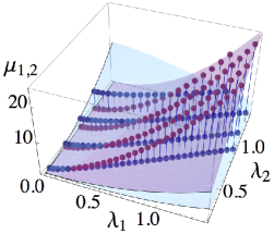
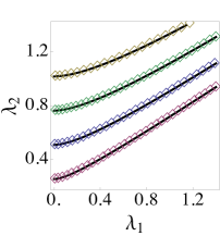
Figure 1: Plots of $(\mu_{1},\mu_{2})$ versus $(\lambda_{1},\lambda_{2})$. On the left, the red and blue surfaces represent $\mu_{1}(\lambda_{i})$ and $\mu_{2}(\lambda_{i})$ in (29) and (30), respectively. The red and blue points represent the numerical data $(\lambda_{1}(\mu_{a}),\lambda_{2}(\mu_{a}),\mu_{b})$ $(b=1,2)$ from the TBA equations, which are solved for given $\mu_{a}=\bar{\mu}_{a}$. Each sequence from the bottom to the top corresponds to $(\mu_{2})^{2/5}=1/2,1,3/2,2$, with $\mu_{1}$ varied. $\lambda_{i}$ are determined by comparing the TBA free energy with the CFT perturbation. On the right, the diamonds ($\diamond$) represent the projections of the left points to the $(\lambda_{1},\lambda_{2})$-plane. The solid lines are the contours in the fundamental domain for $\bigl{(}\mu_{2}(\lambda_{i})\bigr{)}^{2/5}=1/2,1,3/2,2$ from (30).

VIII Mass-coupling relation

To see this, first note that the master formula (24) enables us to calculate the free energy Ward identity,

$$\partial_{i}\bar{\partial}_{j}\mathcal{F}=-\langle\Phi_{ij}\rangle-\int d^{2}x\langle\Psi_{i}(x)\bar{\Psi}_{j}(0)\rangle_{c}=-\frac{5}{2}\langle\Phi_{ij}\rangle\,.$$ (25)

Together with $\mathcal{F}=\mu_{1}\bar{\mu}_{2}+\mu_{2}\bar{\mu}_{1}$, this implies complete factorization, i.e., $\mu_{a}$ depends on $\lambda_{i}$ as $\mu_{a}(\lambda_{1},\lambda_{2})$, and similarly $\bar{\mu}_{a}$ as $\bar{\mu}_{a}(\bar{\lambda}_{1},\bar{\lambda}_{2})$. This means that the original three-variable mass-coupling relation is reduced to two identical copies of the chiral two-variable mass-coupling relation. On dimensional grounds we can thus write

$$\mu_{a}=\frac{\lambda_{1}^{5/2}}{2}q_{a}(\eta)\,,\quad\bar{\mu}_{a}=\frac{\bar{\lambda}_{1}^{5/2}}{2}q_{a}(\bar{\eta})\,,$$ (26)

so as to maintain the left-right symmetry of the problem, where as before $\eta=\lambda_{1}/\lambda_{2}$.

The master formula implies also that

$$v_{i}\partial_{i}\langle\Phi_{kj}\rangle=\int d^{2}x\langle J^{+}(x)\Phi_{kj}\rangle_{c}=\frac{\pi}{2}M_{ki}\langle\Phi_{ij}\rangle\,,$$ (27)

where from the OPEs we obtain $M_{11}=1$, $M_{12}=M_{21}=\frac{1}{2}\eta$ and $M_{22}=0$. Through (23), this actually translates into the following differential equation for $q_{a}$:

$$\eta^{2}\left(1-\frac{\eta^{2}}{3}\right)q_{a}^{\prime\prime}+\eta\left(4-\frac{2\eta^{2}}{3}\right)q_{a}^{\prime}+\frac{5}{4}q_{a}=0\,,$$ (28)

which is a hypergeometric differential equation whose solutions need to be fixed from the boundary conditions. One special case can be obtained by sending $\lambda_{1}=\bar{\lambda}_{1}$ to $0$. In this case only the TCI model is perturbed with $\lambda_{2}\bar{\lambda}_{2}\Phi_{22}$ and the masses are explicitly known as $m_{1}=0$ and $m_{2}=\kappa(\lambda_{2}\bar{\lambda}_{2})^{5/4}$ with $\kappa={56(21\pi)^{1/4}\over 5^{5/2}}\bigl{(}{\Gamma(-\frac{7}{5})\Gamma(\frac{1}{5})\over\Gamma(\frac{12}{5})\Gamma(\frac{4}{5})}\bigr{)}^{5/8}$ Zamolodchikov:1995xk ; Hatsuda:2011ke . The solution of (28) for such vanishing $\mu_{1}$ is unique up to normalization, giving

$$\mu_{1}(\lambda_{1},\lambda_{2})=B\lambda_{1}^{2}(\lambda_{1}+\sqrt{3}\lambda_{2})^{1/2}F\biggl{(}\frac{2\lambda_{1}}{\lambda_{1}+\sqrt{3}\lambda_{2}}\biggr{)}\,,$$ (29)

where $F(z)=\,_{2}F_{1}\left(-\frac{1}{2},\frac{3}{2};3|z\right)$. The $S_{3}$ symmetry then yields

$$\mu_{2}(\lambda_{1},\lambda_{2})=\frac{B}{4}\frac{\left(\sqrt{3}\lambda_{2}-\lambda_{1}\right)^{2}}{(\lambda_{1}+\sqrt{3}\lambda_{2})^{-1/2}}F\biggl{(}\frac{\sqrt{3}\lambda_{2}-\lambda_{1}}{\lambda_{1}+\sqrt{3}\lambda_{2}}\biggr{)}\,.$$ (30)

(29) and (30) hold in the fundamental domain $0\leq\lambda_{1}\leq\sqrt{3}\lambda_{2}$, which are continued outside by the $S_{3}$ symmetry. The normalization is fixed by the above single-mass result: $B=\kappa\frac{5\pi}{16\sqrt[4]{3}}$. This is our main result, which we have checked numerically from the TBA equations CastroAlvaredo:1999em . FIG. 1 shows the agreement of (29), (30), and samples of numerical data. Furthermore, at $(\lambda_{1},\lambda_{2})=(\lambda/2,\sqrt{3}\lambda/2)$, we confirm that $\mu_{1}=\mu_{2}=\frac{B}{2\sqrt{2}}F(1/2)\lambda^{5/2}$, which exactly reproduces the mass-coupling relation in the equal-mass case Fateev:1993av ; Hatsuda:2011ke . The mass-coupling relation enables us to express the free energy density $\mathcal{F}$ in terms of $(\lambda_{i},\bar{\lambda}_{i})$, which then can be used via (25) to obtain the one-point functions of $\Phi_{ij}$.

IX Conclusions

In this letter we developed a new method to calculate the exact mass-coupling relation for multi-scale quantum integrable models. We combined form factor perturbation theory with the construction of conserved tensor currents. The generalization of the $\Theta$ sum rule Ward identity of these currents provided a differential equation for the mass coupling relations, leading to solutions in terms of hypergeometric functions. This is the first result for multi-scale mass-coupling relations. Our work provides the missing link to develop an analytic expansion of ten-particle scattering amplitudes of the four-dimensional maximally supersymmetric gauge theory at strong coupling around a ${\mathbb{Z}}_{10}$-symmetric kinematic point . Although we analyzed here the simplest multi-scale HSG model, the methods can be extended for other multi-scale perturbed CFTs. More details and related results will be reported elsewhere BBIST .

- (1) P. Hasenfratz, M. Maggiore and F. Niedermayer, “The exact mass gap of the O(3) and O(4) nonlinear -models in ,” Phys. Lett. B 245, 522 (1990).
- (2) P. Hasenfratz and F. Niedermayer, “The exact mass gap of the O() -model for arbitrary in ,” Phys. Lett. B 245, 529 (1990).
- (3) A. B. Zamolodchikov, “Thermodynamic Bethe ansatz in relativistic models. Scaling three state Potts and Lee-Yang models,” Nucl. Phys. B 342, 695 (1990).
- (4) P. Forgács, F. Niedermayer and P. Weisz, “The exact mass gap of the Gross-Neveu model (I). The thermodynamic Bethe ansatz,” Nucl. Phys. B 367, 123 (1991).
- (5) P. Forgács, S. Naik and F. Niedermayer, “The exact mass gap of the chiral Gross-Neveu model,” Phys. Lett. B 283, 282 (1992).
- (6) J. Balog, S. Naik, F. Niedermayer and P. Weisz, “Exact mass gap of the chiral SU() SU() model,” Phys. Rev. Lett. 69, 873 (1992).
- (7) V. A. Fateev, E. Onofri and A. B. Zamolodchikov, “Integrable deformations of O(3) sigma model. The sausage model,” Nucl. Phys. B 406, 521 (1993).
- (8) T. J. Hollowood, “The exact mass gaps of the principal chiral models,” Phys. Lett. B 329, 450 (1994).
- (9) J. M. Evans and T. J. Hollowood, “The exact mass gap of the supersymmetric O() sigma model,” Phys. Lett. B 343, 189 (1995).
- (10) J. M. Evans and T. J. Hollowood, “The exact mass gap of the supersymmetric CPn-1 sigma model,” Phys. Lett. B 343, 198 (1995).
- (11) A. B. Zamolodchikov, “Two point correlation function in scaling Lee-Yang model,” Nucl. Phys. B 348, 619 (1991).
- (12) F. Constantinescu and R. Flume, “The convergence of strongly relevant perturbations of conformal field theories,” Phys. Lett. B 326, 101 (1994).
- (13) A. B. Zamolodchikov, “Mass scale in the sine-Gordon model and its reductions,” Int. J. Mod. Phys. A 10, 1125 (1995).
- (14) V. A. Fateev, “The exact relations between the coupling constants and the masses of particles for the integrable perturbed conformal field theories,” Phys. Lett. B 324, 45 (1994).
- (15) C. R. Fernández-Pousa, M. V. Gallas, T. J. Hollowood and J. L. Miramontes, “The symmetric space and homogeneous sine-Gordon theories,” Nucl. Phys. B 484, 609 (1997).
- (16) C. R. Fernández-Pousa, M. V. Gallas, T. J. Hollowood and J. L. Miramontes, “Solitonic integrable perturbations of parafermionic theories,” Nucl. Phys. B 499, 673 (1997).
- (17) C. R. Fernández-Pousa and J. L. Miramontes, “Semiclassical spectrum of the homogeneous sine-Gordon theories,” Nucl. Phys. B 518, 745 (1998).
- (18) J. L. Miramontes and C. R. Fernández-Pousa, “Integrable quantum field theories with unstable particles,” Phys. Lett. B 472, 392 (2000).
- (19) O. A. Castro-Alvaredo, A. Fring, C. Korff and J. L. Miramontes, “Thermodynamic Bethe ansatz of the homogeneous sine-Gordon models,” Nucl. Phys. B 575, 535 (2000).
- (20) P. Dorey and J. L. Miramontes, “Mass scales and crossover phenomena in the homogeneous sine-Gordon models,” Nucl. Phys. B 697, 405 (2004).
- (21) Y. Hatsuda, K. Ito, K. Sakai and Y. Satoh, “Thermodynamic Bethe ansatz equations for minimal surfaces in AdS3,” JHEP 1004, 108 (2010).
- (22) Y. Hatsuda, K. Ito, K. Sakai and Y. Satoh, “-functions and gluon scattering amplitudes at strong coupling,” JHEP 1104, 100 (2011).
- (23) Y. Hatsuda, K. Ito and Y. Satoh, “T-functions and multi-gluon scattering amplitudes,” JHEP 1202, 003 (2012).
- (24) Y. Hatsuda, K. Ito and Y. Satoh, “Null-polygonal minimal surfaces in AdS4 from perturbed W minimal models,” JHEP 1302, 067 (2013).
- (25) L. F. Alday and J. M. Maldacena, “Gluon scattering amplitudes at strong coupling,” JHEP 0706, 064 (2007).
- (26) Č. Crnković, R. Paunov, G. M. Sotkov and M. Stanishkov, “Fusions of conformal models,” Nucl. Phys. B 336, 637 (1990).
- (27) O. A. Castro-Alvaredo, A. Fring and C. Korff, “Form-factors of the homogeneous sine-Gordon models,” Phys. Lett. B 484, 167 (2000).
- (28) O. A. Castro-Alvaredo and A. Fring, “Identifying the operator content, the homogeneous sine-Gordon models,” Nucl. Phys. B 604, 367 (2001).
- (29) G. Delfino, G. Mussardo and P. Simonetti, “Nonintegrable quantum field theories as perturbations of certain integrable models,” Nucl. Phys. B 473, 469 (1996).
- (30) A. B. Zamolodchikov, “Integrals of motion in scaling three state Potts model field theory,” Int. J. Mod. Phys. A 3, 743 (1988).
- (31) A. B. Zamolodchikov, “Integrable field theory from conformal field theory,” Adv. Stud. Pure Math. 19, 641 (1989).
- (32) G. Delfino, P. Simonetti and J. L. Cardy, “Asymptotic factorization of form-factors in two-dimensional quantum field theory,” Phys. Lett. B 387, 327 (1996).
- (33) Z. Bajnok, J. Balog, K. Ito, Y. Satoh and G. Zs. Tóth, “On the mass-coupling relation of multi-scale quantum integrable models,” arXiv:1604.02811[hep-th].