Probing the statistics of transport in the Hénon Map

Abstract

The phase space of an area-preserving map typically contains infinitely many elliptic islands embedded in a chaotic sea. Orbits near the boundary of a chaotic region have been observed to stick for long times, strongly influencing their transport properties. The boundary is composed of invariant “boundary circles.” We briefly report recent results of the distribution of rotation numbers of boundary circles for the Hénon quadratic map and show that the probability of occurrence of small elements of their continued fraction expansions is larger than would be expected for a number chosen at random. However, large elements occur with probabilities distributed proportionally to the random case. The probability distributions of ratios of fluxes through island chains is reported as well. These island chains are neighbours in the sense of the Meiss-Ott Markov-tree model. Two distinct universality families are found. The distributions of the ratio between the flux and orbital period are also presented. All of these results have implications for models of transport in mixed phase space.

In almost all realistic model systems governed by classical mechanics, the phase space consists of a complex mixture of both regular and chaotic orbits Berry1978 ; Tabor1989 ; Meiss1992 . Such dynamics, as depicted in Fig. 1, is characterized by structures on all scales. One of the most surprising consequences of these fractal regions is that chaotic orbits will tend to “stick” to their boundaries for long times Karney1983 ; MacKay1984 ; Chirikov1984 ; Hanson1985 ; Meiss1986a ; Zaslavsky1997 ; Zaslavsky2000 ; Zaslavsky2005 . This occurs even though a long-time average is ergodic, covering equal areas in equal times Meiss1994 . The sticking leads to an observed algebraic decay of correlation functions, Poincaré recurrences and survival times Ceder2013 ; Cristadoro2008 ; Venegeroles2009 .

For the case of two degrees of freedom or equivalently, by Poincaré section, of area-preserving maps, the boundary of a chaotic region consists of infinitely many invariant circles. It is important to note that the existence of such separating circles is a generic property of smooth two-dimensional, area-preserving maps with elliptic orbits according to KAM theory Meiss1992 . These boundary circles are surrounded by leaky partial barriers, called cantori MacKay1984 . The flux of chaotic orbits through the cantori approaches to zero at a boundary, explaining the observed stickiness Meiss1986a . The bottom right panel of Fig. 1 shows a resonance region surrounding a stable (elliptic) fixed point. The broken separatrix of an unstable (hyperbolic) fixed point gives rise to chaos through the famous Smale horseshoe mechanism. There is a trapped region around the stable point bounded by the circle labeled $BC$. Outside this circle are layers associated with periodic orbits of increasing period. Each of the stable periodic orbits in a layer gives rise to a set of islands encircling the original island. One such island, with period $7$, is enlarged in the lower left panel, and it too has a boundary circle, $BC^{\prime}$. This islands-around-islands structure is repeated on ever finer scales in repeated enlargements.

The complex structure results in algebraic decay of the Poincaré recurence and survival probabilities characterized by various exponents Chirikov1984 . Recently, a statistical approach has been offered as a way to explain the distribution of these exponents Cristadoro2008 ; Ceder2013 ; Alus2014 . The question of how to build such a statistical description is the main objective of this paper. Additional details, given in Alus2014 , are reviewed briefly. Additional discussion of the averaging procedure, and the differences between different ensembles is given in Alus2015 . The model of transport that we use is the Markov tree, first proposed in Meiss1986a . The construction of this model relies on characterizing: (1) the boundary circles, and (2) the flux ratios between adjacent island chains on the tree. Together these give a representation of the distribution of transmission rates between different nodes on the tree. For this investigation, we use Hénon’s iconic area-preserving, quadratic map of the plane Henon1969 ; it is a one-parameter family that can be written in the form

$$(x^{\prime},y^{\prime})=T(x,y)=(-y+2K-2x^{2},x).$$ (1)

Continued fraction coefficients: First we examine characterization of boundary circles. We will show that these circles are characterized by rotation numbers that have unusual continued fraction expansions, following on the pioneering study of Greene, MacKay and Stark (GMS) Greene1986 . Although we focus on the main (class-one Meiss1986 ) circles, the results apply also to boundary circles on finer scales, like the (class-two) circle $BC^{\prime}$ in the figure, and therefore is conjectured to be universal Alus2014 .

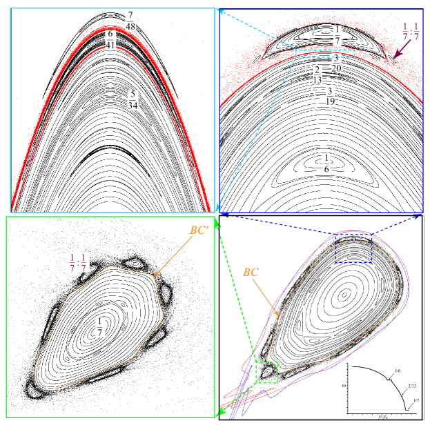
Figure 1: Phase space of (1) for $K=-0.17197997940$ showing a hierarchy of scales. The bottom right panel shows the fixed point island and the stable (blue) and unstable (red) manifolds of the hyperbolic fixed point. An enlargement of a period-$7$ island is in the bottom left panel. The top right enlarges a region near the boundary circle showing the first outer approximant, $\tfrac{1}{7}$, to the boundary circle rotation number $\omega_{BC}$ as well as other island chains. The final zoom (top left) shows the next inner, $\tfrac{5}{34}=[0;6,1,4]$, and outer, $\tfrac{6}{41}=[0;6,1,4,1]$, approximants. Red points in the upper panels are orbits in the unbounded chaotic component.

A boundary circle separates an outer region, where orbits can escape from the resonance, from an inner region, where orbits are trapped near an elliptic orbit. Though a boundary circle is isolated from the outside, every interior neighborhood typically contains other invariant circles that also encircle the elliptic point. Nevertheless, between each pair of invariant circles there are chaotic layers, as well as periodic orbits. GMS showed that the rotation number of a typical boundary circle has unusual number theoretic properties. Recall that any real number $\omega$ has a continued fraction expansion

$$\omega=m_{0}+\frac{1}{m_{1}+\frac{1}{m_{2}+\ldots}}=[m_{0};m_{1},m_{2},\ldots]$$ (2)

where $m_{0}\in{\mathbb{Z}}$ and $m_{i}\in{\mathbb{N}}$ Khinchin1964 . When $\omega$ is irrational, this expansion is infinite, and a truncation after $i$ terms gives a rational, $\omega_{i}=\frac{p_{i}}{q_{i}}=[m_{0};m_{1},m_{2},\ldots,m_{i}]$ called the $i^{th}$ convergent to $\omega$. The convergents are alternately larger than and smaller than $\omega$ Khinchin1964 . For a typical resonance, $m_{0}=0$ and the rotation number will be a decreasing function of distance from the elliptic fixed point, an example is shown in the inset in Fig. 1. Equation (2) implies that $\omega_{1}=\tfrac{1}{m_{1}}$ and $\omega_{2}=\tfrac{m_{2}}{m_{1}m_{2}+1}$ so that $\omega_{1}>\omega>\omega_{2}$; more generally one can see that the convergents in the outer region will correspond to even $i$. For example, in Fig. 1, $\omega_{BC}=[0;6,1,4,1,5,1,2,1,\ldots]$. The first convergent $\tfrac{p_{1}}{q_{1}}=\tfrac{1}{6}=[0;6]$, gives rise to a period-$6$ island chain in the trapped region, while the second $\tfrac{1}{7}=[0;6,1]$ gives a chain embedded in the outer, chaotic component. Subsequent even convergents, e.g., $\tfrac{6}{41}=[0;6,1,4,1]$, result in smaller islands closer to the boundary circle, see the upper left panel of the figure.

GMS computed the coefficients $m_{i}$ for the rotation numbers of boundary circles and found that they differed from the distribution that would occur if they were selected at random from $[0,1]$ with uniform measure, namely, the Gauss-Kuzmin (GK) distribution Khinchin1964 , $p_{GK}(m)=-\log_{2}\left(1-\frac{1}{(1+m)^{2}}\right)$. In contrast to $p_{GK}$, GMS conjectured that for the even (outer) coefficients only the elements $m_{i}=1$ and $2$ occur, while for the odd (inner) coefficients $m_{i}\leq 5$.

We explored in Alus2014 the distribution of the continued fraction elements, for the Hénon map (1) for a much larger sample and for longer continued fraction expansions than were computed by GMS. The empirical probability mass function, $p_{BC}(m)$, the frequency of occurrence of $m\in{\mathbb{N}}$ (both inner and outer) in the resulting list of coefficients $m_{i}$, is shown in Fig. 2. In the right panel of this figure, we eliminate the coefficients with $i\leq 4$, as the first few coefficients may be expected to depend on the map’s details, while the deeper approximants should be more universal. Nevertheless, the distributions are of similar nature.

           

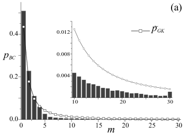
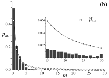
Figure 2: Distribution of continued fraction elements for the Hénon fixed point boundary circle with $K\in(-0.25,0.75)$ compared with the conditional the GK distribution $\tilde{p}_{GK}$: (a) all coefficients and (b) those for $i>4$. Fig 8 of Alus2014

For the outer coefficients we find very few $m_{i}>3$; the largest that we found is $m_{i}=8$. We found inner elements as large as $48$. Both of these distributions deviate from those of GMS Alus2014 . In particular it appears that the inner elements are unbounded. While the results deviate significantly from the Gauss-Kuzmin distribution for small $m$, the distribution appears to be a fixed fraction of the Gauss-Kuzmin distribution for larger $m$, i.e., $p_{BC}(m)$ is proportional to $\tilde{p}_{GK}(m)$ when $m>5$.

Though we expect that the rotation number of each boundary circle should satisfy a Diophantine property Greene1986 , and have bounded coefficients Khinchin1964 , there is not necessarily a uniform bound for different numbers. We therefore conjecture that no bound exists for the continued fraction elements. Furthermore, even though the one-sided isolation of a boundary circle leads to an abundance of coefficients with smaller $m$ values, larger values appear to follow a fixed fraction of the GK distribution.

Flux ratios: Next we turn to the question of flux ratios between adjacent island chains represented by neighboring sites on the binary Markov tree model. The fluxes, $\Delta W$, through an island chain are calculated by subtracting the action of the hyperbolic orbit from that of the elliptic one (see Alus2014 ). These fluxes give the first step for a theory of transport in phase space, namely, the area that escapes/enters a region around a periodic island chain in one period. We mark fluxes of island chains represented by different nodes on the tree using $\Delta W_{S}$, where $S$, an index representing the node on the tree, and is a binary number. Daughter nodes are denoted by $Si$ with $i\in\{0,1\}$.

After introducing a new variable, $v_{S}=-\ln w_{S}$ where $w_{S}=\frac{\Delta W_{Si}}{\Delta W_{S}}$, we find two universality families that are described by distinct distributions regardless of the site position. First is $v^{class}$, as in Meiss1986 , for the ratio between two chains encircling one another, i.e., one is a convergent to the boundary circle of the other. The second is $v^{level}$, as in MacKay1993 , for the ratio between two chains which are part of a family that converges to the same boundary circle. We find that different regimes of the parameter of (1), have similar distributions (see Fig. 3). Since the Hénon map is often used as an approximation for dynamics in the proximity of a resonance, this might indicate the universality of these distributions.

           

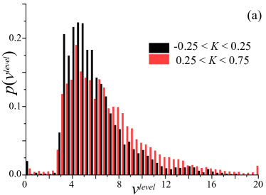
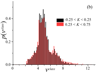
Figure 3: (Color online) Probability distributions of the log-flux ratio $\nu_{S}$. (a) Distribution of $v^{level}$, corresponding to right-going transitions $S\to S1$ for $S$ using bins of size $0.4$. (b) Distribution of $v^{class}$, corresponding to left-going transitions, $S\to S0$ using bins of size $0.2$. The shades (black and red) show two ranges of $K$ as indicated. Fig 10 of Alus2014

Time scaling ratios: An important scaling for the Markov tree model is the time scaling between two adjacent sites, $\varepsilon_{S}=q_{S}/q_{Si}$ where $q_{S}$ is the period of the orbit in state $S$. For the level transitions, this ratio is determined by the continued fraction expansion coefficients for the boundary circle. For class transitions, this ratio is determined by the relative period of the outermost chain of islands around a higher class boundary circle. The two ratios $w_{s}$ and $\varepsilon_{S}$ are highly correlated, and it is convenient to define the ratio $\xi_{S}=\ln\left({w_{S}}\right)/\ln\left({\varepsilon_{S}}\right)$.

The empirical distributions of $\xi^{level}$ and $\xi^{class}$, presented in Fig. 4, have mean values 3.78 and 2.33, respectively. For comparison, Meiss1986a used fixed values 3.05 and 2.19, taken from Greene1986 , for class-zero boundary circles, and Meiss1986 , for class renormalization in a self-similar phase space with period-$7$ islands. This suggest that the self-similar phase space values do give an appropriate approximation. However, it is interesting that while level scaling distributions GMS obtained for the standard map are symmetric about their means, ours—for the Hénon map—have long, positive tails, as can be seen from Fig. 3 and Fig. 4.

           

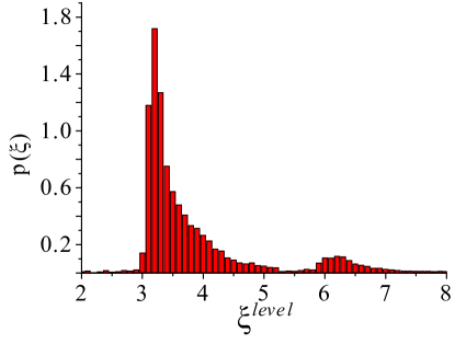
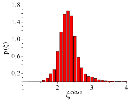
Figure 4: the distributions of $\xi^{level}$ and $\xi^{class}$ for parameters used in Fig. 3

In Summary: Probability distributions of the continued fraction expansion elements of boundary circle were calculated, showing that the elements are not bounded contrary to previous conjectures. Probabilities of flux ratios between adjacent sites on the binary Markov tree proposed by Meiss and Ott Meiss1986a were shown to be parameter independent and to indicate two possible universal distributions. Finally, histograms for the exponent $\xi$ have mean values that are similar to previous results calculated for fine tuned parameters. These provide support to the validity of the Meiss-Ott Markov-tree model, and might be used in order to calculate corrections to it.

Acknowledgments: The work was supported in part by the Israel Science Foundation (ISF) grant number 1028/12, by the US-Israel Binational Science Foundation (BSF) grant number 2010132, by the Shlomo Kaplansky academic chair, and by National Science Foundation (NSF) grant DMS-1211350. SF also thanks the Kavli Institute for Theoretical Physics (KITP) in Santa Barbara for its hospitality, where this research was supported in part by NSF grant PHY11-25915. We would like to thank Ed Ott for fruitful discussions and Tassos Bountis for the invitation to contribute to this special issue.

References

- [1] M.V. Berry. Regular and irregular motion. In S. Jorna, editor, Topics in Nonlinear Dynamics, volume 46 of AIP Conf. Proc., pages 16–120. AIP, New York, 1978.
- [2] M. Tabor. Chaos and Integrability in Nonlinear Dynamics : an Introduction. J. Wiley, New York, 1989.
- [3] J.D. Meiss. Symplectic maps, variational principles, and transport. Rev. Mod. Phys., 64(3):795–848, July 1992.
- [4] C.F.F. Karney. Long-time correlations in the stochastic regime. Physica D, pages 360–380, 1983.
- [5] R.S. MacKay, J.D. Meiss, and I.C. Percival. Transport in Hamiltonian systems. Physica D, 13(1-2):55–81, Aug 1984.
- [6] B.V. Chirikov and D.L. Shepelyansky. Correlation properties of dynamical chaos in Hamiltonian systems. Physica D, pages 395–400, 1984.
- [7] J.D. Hanson, J.R. Cary, and J.D. Meiss. Algebraic decay in self-similar Markov chains. J. Stat. Phys., 39(3-4):327–345, May 1985.
- [8] J.D. Meiss and E. Ott. Markov tree model of transport in area-preserving maps. Physica D, 20(2-3):387–402, June 1986.
- [9] G.M. Zaslavsky, M. Edelman, and B.A. Niyazov. Self-similarity, renormalization, and phase space nonuniformity of Hamiltonian chaotic dynamics. Chaos, 7(1):159–181, March 1997.
- [10] G.M. Zaslavsky and M. Edelman. Hierarchical structures in the phase space and fractional kinetics: I. Classical systems. Chaos, 10(1):135–146, March 2000.
- [11] G.M. Zaslavsky. Hamiltonian Chaos and Fractional Dynamics. Oxford Univ. Press, Oxford, 2005.
- [12] J.D. Meiss. Transient measures for the standard map. Physica D, 74(3 & 4):254–267, 1994.
- [13] R. Ceder and O. Agam. Fluctuations in the relaxation dynamics of mixed chaotic systems. Phys. Rev. E, 87(1):012918, January 2013.
- [14] G. Cristadoro and R. Ketzmerick. Universality of algebraic decays in Hamiltonian systems. Phys. Rev. Lett., 100(18):184101, May 2008.
- [15] R. Venegeroles. Universality of algebraic laws in Hamiltonian Systems. Phys. Rev. Lett., 102(6):064101, February 2009.
- [16] O. Alus, S. Fishman, and J.D. Meiss. Statistics of the island-around-island hierarchy in Hamiltonian phase space. Phys. Rev. E, 90:062923, Dec 2014.
- [17] O. Alus and S. Fishman. Diffusion for ensembles of standard maps. Phys. Rev. E, 92:042904, Oct 2015.
- [18] M. Hénon. Numerical study of quadratic area-preserving mappings. Q. J. Appl. Math., 27:291–312, 1969.
- [19] J.M. Greene, R.S. MacKay, and J. Stark. Boundary circles for area-preserving maps. Physica D, 21(2-3):267–295, September 1986.
- [20] J.D. Meiss. Class renormalization: islands around islands. Phys. Rev. A, 34(3), 1986.
- [21] A.Y. Khinchin. Continued Fractions. University of Chicago Press, Chicago, 1964.
- [22] R.S. MacKay. Renormalization in Area-Preserving Maps. Adv. Ser. Lin. Dynam. World Scientific, Singapore, 1993.