Correlations between compositions and orbits
established by the giant impact era of planet formation

Abstract

The giant impact phase of terrestrial planet formation establishes connections between super-Earths’ orbital properties (semimajor axis spacings, eccentricities, mutual inclinations) and interior compositions (the presence or absence of gaseous envelopes). Using $N$-body simulations and analytic arguments, we show that spacings derive not only from eccentricities, but also from inclinations. Flatter systems attain tighter spacings, a consequence of an eccentricity equilibrium between gravitational scatterings, which increase eccentricities, and mergers, which damp them. Dynamical friction by residual disk gas plays a critical role in regulating mergers and in damping inclinations and eccentricities. Systems with moderate gas damping and high solid surface density spawn gas-enveloped super-Earths with tight spacings, small eccentricities, and small inclinations. Systems in which super-Earths coagulate without as much ambient gas, in disks with low solid surface density, produce rocky planets with wider spacings, larger eccentricities, and larger mutual inclinations. A combination of both populations can reproduce the observed distributions of spacings, period ratios, transiting planet multiplicities, and transit duration ratios exhibited by Kepler super-Earths. The two populations, both formed in situ, also help to explain observed trends of eccentricity vs. planet size, and bulk density vs. method of mass measurement (radial velocities vs. transit timing variations). Simplifications made in this study — including the limited timespan of the simulations, and the approximate treatments of gas dynamical friction and gas depletion history — should be improved upon in future work to enable a detailed quantitative comparison to the observations.

1. Introduction

The Kepler Mission discovered thousands of candidate “super-Earths,” planets between the size of Earth and Neptune (e.g., Borucki et al. 2011a, b; Batalha et al. 2013; Burke et al. 2014; Mullally et al. 2015). They exhibit a wide range of bulk densities, anywhere from $\sim$10 g/cm³ to less than that of water (e.g., Carter et al. 2012; Wu & Lithwick 2013; Lopez & Fortney 2014; Weiss & Marcy 2014; Dressing et al. 2015; Wolfgang et al. 2015). Much of our knowledge of their orbital properties comes from the subset of systems each containing two or more transiting planets. Statistical studies have found that systems of multiple super-Earth “tranets” (planets that transit; Tremaine & Dong 2012) have small eccentricities (Moorhead et al., 2011; Wu & Lithwick, 2013; Hadden & Lithwick, 2014; Van Eylen & Albrecht, 2015) and small mutual inclinations (Fang & Margot, 2012b; Figueira et al., 2012; Fabrycky et al., 2014) of a few percent or less.

The orbital spacings of tranets (Lissauer et al., 2011; Fang & Margot, 2013; Fabrycky et al., 2014; Lissauer et al., 2014; Malhotra, 2015; Steffen, 2016) have been a particular focus for theoretical studies of formation (Hansen & Murray, 2013; Petrovich et al., 2014; Malhotra, 2015), stability (Pu & Wu, 2015), dynamical excitation (Tremaine, 2015), and migration (Lithwick & Wu, 2012; Batygin & Morbidelli, 2013; Delisle & Laskar, 2014; Goldreich & Schlichting, 2014; Hands et al., 2014; Chatterjee & Ford, 2015; Deck & Batygin, 2015). In this paper, we define the spacing

$$\Delta\equiv\frac{\delta a}{R_{\rm H}}$$ (1)

as the semi-major axis difference $\delta a\equiv a_{2}-a_{1}$ between adjacent planets, normalized by their mutual Hill radius:

$$R_{\rm H}\equiv\frac{a_{1}+a_{2}}{2}\left(\frac{M_{{\rm p},1}+M_{{\rm p},2}}{3M_{\star}}\right)^{1/3},$$ (2)

where $a$ is the semi-major axis, $M_{\rm p}$ is the planet mass, and $M_{\star}$ is the stellar mass. The tranet spacing distribution peaks at $\Delta\sim 20$. Fang & Margot (2013) found a similar spacing distribution for the underlying planets, assuming a single population of planetary systems drawn from independent distributions of mutual inclinations, spacings, multiplicities, and planet sizes. Planet spacings of $\Delta\sim 20$ — shrinking to $\Delta\sim 12$ for the highest multiplicity systems — lie safely outside the empirical stability limit of $\Delta\sim 10$ (Chambers et al., 1996; Yoshinaga et al., 1999; Zhou et al., 2007; Smith & Lissauer, 2009; Fang & Margot, 2012a; Lissauer et al., 2014; Pu & Wu, 2015). Studies of tranet multiplicity — a property that depends on both spacing and mutual inclination — have found a “Kepler dichotomy,” i.e., a need for two populations to account for an apparent excess of single tranet systems over multi-tranet systems (Lissauer et al., 2011; Johansen et al., 2012; Hansen & Murray, 2013; Ballard & Johnson, 2014; Moriarty & Ballard, 2015).

Here we explore how the orbital properties of super-Earths — their spacings, eccentricities, and inclinations — originate from the circumstances of their formation from primordial disks of solids and gas. We will uncover correlations between these orbital properties and planet compositions (gas-enveloped vs. rocky), correlations that are not due to observational bias and that are currently neglected in Kepler population studies (e.g., Lissauer et al. 2011; Fang & Margot 2012b; Figueira et al. 2012; Tremaine & Dong 2012; Fang & Margot 2013; Ballard & Johnson 2014; Fabrycky et al. 2014; Steffen 2016). We work in the context of in-situ formation (e.g., Hansen & Murray 2012, 2013; Chiang & Laughlin 2013; Lee et al. 2014; Dawson et al. 2015; Lee & Chiang 2015, 2016; Moriarty & Ballard 2015; see also Inamdar & Schlichting 2015), simulating the assembly of super-Earths starting from isolation masses.

We devote especial attention to the origin of super-Earth spacings. The spacing distributions of planets and protoplanets have been explored theoretically from several vantage points. One consideration is stability. The timescale for orbit crossing is known empirically to increase exponentially with the Hill spacing $\Delta$ (Yoshinaga et al., 1999; Zhou et al., 2007; Pu & Wu, 2015). The spacing must be wide enough for the orbit crossing time to exceed the system’s age. Tremaine (2015) presented another point of view from statistical mechanics. Other perspectives derive from considerations of planet formation. For isolation masses (a.k.a. oligarchs) accreting small bodies in their feeding zones, a spacing equilibrium is achieved between mass growth, which decreases the separation in Hill radii, and orbital repulsion driven by gravitational (a.k.a. viscous) stirring (Kokubo & Ida, 1995, 1998). In the particle-in-a-box approximation for planet formation by coagulation of small bodies (e.g., Safronov & Zvjagina 1969; Greenzweig & Lissauer 1990; Ohtsuki 1992; Ford et al. 2001; Goldreich et al. 2004; Ida et al. 2013; Petrovich et al. 2014; Johansen et al. 2012; Morrison & Malhotra 2015), random velocities are limited to the surface escape velocity $v_{\rm esc}$ from the most massive body. Schlichting (2014) applied this principle to estimate the minimum disk masses required to form super-Earths in situ. A planet that excites the random velocities of surrounding bodies to the maximum value of $v_{\rm esc}$ has a feeding zone of full width

$$\Delta=\frac{2v_{\rm esc}}{nR_{\rm H}}\simeq 45\left(\frac{P}{\rm yr}\right)^{1/3}\left(\frac{\rho}{{\rm g\,cm}^{-3}}\right)^{1/6},$$ (3)

where $n$ is the planet’s orbital angular frequency (a.k.a. mean motion), $P=2\pi/n$ is the orbital period, and $\rho$ is the planet’s bulk density. This feeding zone width also corresponds to the expected maximum spacing between nascent planets. We will take a related approach by finding the spacing that allows for an “eccentricity equilibrium”: one that balances gravitational scatterings between protoplanets, which excite eccentricities, with mergers, which damp them.

Our paper, which explores how the orbital spacings of super-Earths are fossil records of their formation in situ, and how orbital properties in general are correlated with planet composition, is organized as follows. In Section 2, we describe the setup for the $N$-body simulations that are the basis for all subsequent sections. In Section 3, we show how spacings, eccentricities, and inclinations evolve with time for a few illustrative, gas-free simulations. In particular, we demonstrate how the evolution is sensitive to initial inclinations — an input parameter that, to our knowledge, is not often highlighted as a controlling parameter in coagulation calculations. We offer order-of-magnitude scalings to understand these results, explaining the dependence of spacings on inclinations in terms of an eccentricity equilibrium that balances scatterings with mergers. Section 4 gives a more complete overview of our gas-free simulations, detailing how final spacings depend on various initial conditions. Section 5 brings dynamical friction by disk gas into the mix; we investigate how gas can establish those initial conditions that were assumed in preceding sections. Including gas also enables us to connect planet compositions — whether or not planets have volumetrically significant gas envelopes — with orbital properties; this is the focus of Section 6. Comparisons with observations are made in Section 7; there we will find that we need a mixture of dynamically hot and dynamically cold populations to more faithfully reproduce Kepler data. We present our conclusions in Section 8.

2. Initial conditions for $N$-body simulations

To assess how orbital spacings depend on conditions during the late stages of planet formation, we simulate the growth of isolation mass embryos to super-Earths via collisions (a.k.a. giant impacts). Building on work by, e.g., Chambers et al. (1996), Kokubo & Ida (1998, 2002), Hansen & Murray (2012, 2013), and Dawson et al. (2015), we perform $N$-body integrations each lasting 27 Myr using the hybrid symplectic integrator of mercury6 (Chambers, 1999). The time step is 0.5 days and a close encounter distance (which triggers a switch from the symplectic integrator to the Burlisch-Stoer integrator) is 1 $R_{\rm H}$. We run several thousands of simulations, grouped into ensembles and summarized in Table 1. The default number of simulations per ensemble is 80.

Our simulations begin with embryos each having an isolation mass $M_{\rm emb}$:

$$M_{\rm emb}=0.16M_{\oplus}\left(\frac{\Delta_{0}}{10}\right)^{3/2}\left(\frac{\Sigma_{z,1}}{10\,{\rm g}/{\rm cm}^{2}}\right)^{3/2}$$

$$\times\left(\frac{a}{{\rm AU}}\right)^{3(2+\alpha)/2}\left(\frac{M_{\star}}{M_{\odot}}\right)^{-1/2}$$ (4)

where $\Sigma_{z}=\Sigma_{z,1}(a/{\rm AU})^{\alpha}$. We explore a large range of $\Sigma_{z,1}=3$–400 g/cm². By default, we use an initial spacing $\Delta_{0}=10$, similar to Hansen & Murray (2012, 2013), and based on the Kokubo & Ida (1998, 2002) simulations of embryos formed via the accretion of small bodies. We list the range of the initial number of embryos per simulation, $N_{\rm emb,0}$, and the final number of planets, $N_{\rm p,final}$, in Table 1. Some of our simulations include damping by residual disk gas; these are detailed in Section 5. We assign planets constant bulk densities $\rho$ that define their physical cross sections. When two embryos touch, we assume perfect accretion with no fragmentation.

Initial eccentricities and inclinations are specified in Table 1. Depending on the ensemble, the magnitude of the initial eccentricity $e_{0}$ is set either to 0; to a constant fraction (specified in the Table) of ${h\equiv[(M_{\rm emb,1}+M_{\rm emb,2})/(3M_{\star})]^{1/3}}$, where the subscripts “1” and “2” refer to adjacent inner and outer bodies; or to a constant fraction of the orbital separation ${\delta a/a\equiv(a_{2}-a_{1})/[2(a_{2}+a_{1})]}$. Flat ensembles (Ef, Eci0) are strictly 2D, beginning with and maintaining $i=0$. For other ensembles, the magnitude of the initial inclination $i_{0}$ is drawn either from a uniform distribution between 0–0.1^∘ or 0–0.001^∘; set to a constant value $e_{0}/\sqrt{2}$ (equipartition); or set to $0.01h$. The initial mean anomaly, argument of periapse, and longitude of ascending node are drawn randomly from a uniform distribution spanning 0–2$\pi$. In the remainder of this work, we compute the reported $i$ of each planet relative to the initial $i=0$ plane.

Following Hansen & Murray (2012, 2013), the inner edge of the disk of embryos is drawn randomly from a uniform distribution spanning 0.04–0.06 AU. Other embryos are spaced $\Delta_{0}$ away from each other, up to a maximum $a$ of 1 AU. Embryos are initially placed in order of increasing $a$. The semi-major axis $a_{j}$ and mass $M_{{\rm emb},j}$ of the $j$th embryo are computed from the mutual Hill radius of the previous embryo, i.e., $R_{\rm H}=a_{j-1}\left(\frac{2M_{{\rm emb},j-1}}{3M_{\star}}\right)^{1/3}$. As a result, the actual initial orbital spacings differ slightly from the values of $\Delta_{0}$ listed in Table 1. The surface density normalization $\Sigma_{z,1}$ for each simulation in the ensemble is drawn from a uniform log distribution spanning the range specified in Table 1. The surface density slope $\alpha=-3/2$ except for ensemble Eh$\alpha$-2, which uses $\alpha=-2$, as noted in Table 1.

Table 1Ensembles of Simulations

Name	$e_{0}$	$i_{0}$	$\Delta_{0}$	$\Sigma_{z,1}$	$N_{\rm emb,0}$	$N_{\rm p,final}$	Notes
		(rad)	$(R_{\rm H})$	(g cm-2)
Ef	0	0	10	33–90	22–35	7–13
E	0	$0.1^{\circ}$	10	33–90	22–35	4–11	a
Eh	$\sqrt{2}h/\sqrt{3}$	$e_{0}/\sqrt{2}$	10	3–403	12–128	2–22	b,c
Eh$\alpha$-2	$\sqrt{2}h/\sqrt{3}$	$e_{0}/\sqrt{2}$	10	33–55	19–25	6–8	c,d
Eh$\rho$	$\sqrt{2}h/\sqrt{3}$	$e_{0}/\sqrt{2}$	10	116	20–23	4–7	c,e
Ec	$\delta a/(2a)$	$e_{0}/\sqrt{2}$	10	33–90	22–35	4–10	f
Eci0	$\delta a/(2a)$	0	10	33–90	22–35	5-11	f
Eci0.1	$\delta a/(2a)$	$0.1^{\circ}$	10	33–90	22–35	4–8	a,f
Eci0.001	$\delta a/(2a)$	$0.001^{\circ}$	10	33–90	22–35	4-12	a,f
Ece0.3	$0.3\delta a/a$	$e_{0}/\sqrt{2}$	10	33–90	22–35	4–9	f
Ece0.1	$0.1\delta a/a$	$e_{0}/\sqrt{2}$	10	33–90	22–35	4–9	f
Ece0.3i0.1	$0.3\delta a/a$	$0.1^{\circ}$	10	33–90	22–35	5–8	a,f
Ece0.1i0.1	$0.1\delta a/a$	$0.1^{\circ}$	10	33–90	22–35	5–10	a,f
E$\Delta$3	0	$0.1^{\circ}$	3	33–90	129–240	5–9	a
E$\Delta$5	0	$0.1^{\circ}$	5	33–90	62–111	5–8	a
E$\Delta$7.5	0	$0.1^{\circ}$	7.5	33–90	34–54	4–8	a
E$\Delta$9	0	$0.1^{\circ}$	9	33–90	27–43	3–8	a
E$\Delta$11.5	0	$0.1^{\circ}$	11.5	33–90	19–33	4–12	a
E$\Delta$13	0	$0.1^{\circ}$	3	33–90	17–28	3–14	a
Ed100	$h$	$h/100$	3	38–105	123–220	2–9	c,g
Ed101	$h$	$h/100$	3	38–105	123–220	3–9	c,g
Ed102	$h$	$h/100$	3	38–105	123–220	3–18	c,g
Ed103	$h$	$h/100$	3	38–105	123–220	2–9	c,g
Ed104	$h$	$h/100$	3	38–105	123–220	2–9	c,g

• Inclinations drawn randomly from a uniform distribution between 0 and $i_{0}$.

• Contains 500 simulations. The default is 80.

• $h\equiv[(M_{{\rm p},1}+M_{{\rm p},2})/(3M_{\ast})]^{1/3}$ is the Hill parameter.

• Surface density power-law slope is $\alpha=-2$ instead of the default $\alpha=-3/2$.

• The planet bulk density $\rho$ is drawn from a uniform log distribution from 0.02–14 g cm^-3. The default is a fixed $\rho=1$ g cm^-3.

• $\delta a\equiv a_{2}-a_{1}$ is the semi-major axis difference between neighboring embryos.

• Includes gas damping. See Section 5.

3. Growth and equilibration of eccentricities and spacings

During the giant impact stage of planet formation, planets scatter and merge, establishing the system’s orbital spacings and eccentricities. Through mutual gravitational interactions, planets convert Keplerian shear into random velocity, leading to growth in $e$ and $i$. Mergers (inelastic collisions) counter the growth of random velocities and stabilize the system by widening the spacings between bodies. Figure 1 (row 1) compares the average eccentricity growth from two ensembles of simulations (E, Ef), two individual members of which are shown in Figure 2. Planets begin as moon-to-Mars mass embryos on circular orbits and grow in mass, separation, and eccentricity. Fig. 1 shows four stages for eccentricity growth: the initial growth at low $e$ (stage 1), a faster growth as $e$ approaches orbit crossing (stage 2), growth during orbit crossing (stage 3), and an eccentricity equilibrium (stage 4). For the non-flat ensemble, the average inclination is also plotted in Figure 1. The second row of Figure 1 shows the evolution of $\Delta$, the spacing in mutual Hill radii, which is flat throughout the first two eccentricity growth stages when mergers do not yet occur.

In this section we use order-of-magnitude calculations to understand how eccentricities, inclinations, and orbital spacings are connected. We focus exclusively on the latter phases of the evolution — stages 3 and 4 — when mergers occur and spacings $\Delta$ evolve from their initial values.

Figure 1.— Inclinations matter for orbital spacings. Top: Evolution of $e$ (thick curves) and $i$ (thin curve), averaged over all planets in an ensemble. Averages from the non-flat ensemble E are plotted as red dashed curves and from flat ensemble Ef as a black solid curve; $i$ does not appear on the plot for Ef because that ensemble is completely 2D $(i=0)$. For both ensembles, the eccentricity undergoes four stages of evolution, as demarcated by vertical dotted lines. Middle: Same for Hill spacings $\Delta$ for adjacent pairs of planets. Planet pairs in the flat ensemble (black solid) end up with tighter spacings. Bottom: Distributions of final $\Delta$.

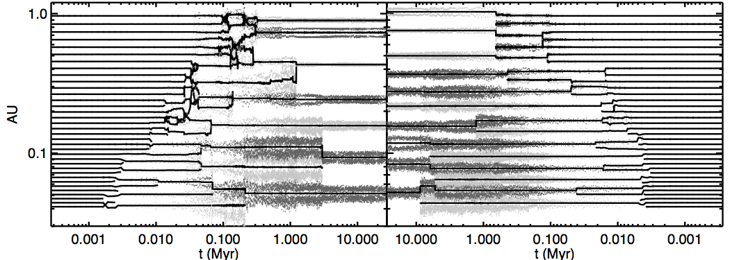
Figure 2.— Evolution of $a$ (black) and $a(1\pm e)$ (gray). Left: $\Sigma_{z,1}=55$ g/cm² simulation from Eh. The final planets have $1.5<M_{p}<5M_{\oplus}$. Right: Identical simulation with initial $i=0$. The planets end up more tightly spaced (in both $a$ and $\Delta$).

3.1. Eccentricity growth rate

We derive an order-of-magnitude formula for eccentricity growth for use in later subsections when we consider the specifics of stages 3 and 4. Consider widely-spaced, shear-dominated pairs for which the relative velocities are

$$v_{\rm rel}\sim v_{\rm H}\Delta,$$ (5)

where $v_{\rm H}$ is the mutual Hill velocity. The relative velocity changes impulsively every conjunction. An encounter between two planets each of mass $M_{\rm p}$ at impact parameter $x$ produces an acceleration

$$\frac{GM_{\rm p}}{x^{2}}=\frac{3n^{2}R_{\rm H}^{3}}{2x^{2}}$$

over a time interval $2x/v_{\rm rel}$, changing $v_{\rm rel}$ by

$$\delta v_{\rm rel}=\frac{3n^{2}R_{\rm H}^{3}}{xv_{\rm rel}}.$$ (6)

It is assumed that $\delta v_{\rm rel}$ is randomly directed; over many encounters, $v_{\rm rel}$ random walks. For a given $x$, the expected number of synodic periods $N_{\rm synodic}$ (i.e., the number of conjunctions or random walk steps) required to change $v_{\rm rel}$ by a fractional amount $f$ is given by

$$\frac{1}{N_{\rm synodic}}=\left(\frac{\delta v_{\rm rel}}{fv_{\rm rel}}\right)^{2}=\frac{9R_{\rm H}^{2}}{f^{2}x^{2}\Delta^{4}}.$$ (7)

Eqn. 7 gives a rate of viscous stirring, which we now average over the geometry of possible impact parameters $x$ from $x_{\rm min}$ to $x_{\rm max}$. The probability of an encounter with impact parameter $x$ depends on the value of $x$ relative to the “scale height” $ia$, as depicted in Figure 3. The scale height for a pair of bodies reflects the range of mutual inclinations resulting from their inclinations $\sim i$ with respect to the initial plane and their range of nodal orientations. Let $D$ be the range of horizontal separations, determined by $\Delta$ and the eccentricity vectors. For $x>ia$, the dynamics is essentially 2D (i.e., in a common orbital plane) and independent of the inclinations. If orbits are crossing (Figure 3, right panel), the probability of a conjunction occurring within the interval $x$ and $x+dx$ for $x>ia$ is

$$p(x)dx=\frac{4x\sin^{-1}\left(ia/x\right)dx}{2iaD}\sim\frac{2dx}{D},\,\,\,\,x>ia,\,{\rm crossing}.$$

For non-crossing orbits (Figure 3, left panel), this 2D probability is reduced by a factor of 2. For $x<ia$ (the 3D case), the corresponding probability is

$$p(x)dx=\frac{2\pi x\,dx}{2iaD}\sim\frac{\pi x\,dx}{iaD},\,\,\,\,x<ia,$$

reduced by a factor of $\pi x/(2ia)$ relative to the 2D case and dependent on $i$.

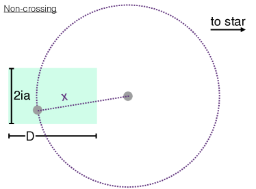
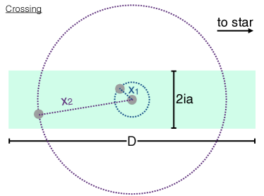
Figure 3.— The probability of an encounter with impact parameter $x$ between two bodies depends on the value of $x$ relative to the scale height $ia$. The rectangle represents the area of possible encounter space for the pair of bodies. Left: Non-crossing orbits. The probability of an encounter within $dx$ of $x$ is $\frac{2x\sin^{-1}\left[ia/x\right]dx}{iaD}\sim\frac{dx}{D}$. Right: Crossing orbits. For $x_{1}<ia$, the probability of an encounter within $dx$ of $x_{1}$ is $\frac{2\pi x_{1}dx}{2iaD}\sim\frac{x_{1}dx}{iaD}$, where $D$ is the range of horizontal separations. For $x_{2}>ia$, the probability of an encounter within $dx$ of $x_{2}$ is $\frac{4x_{2}\sin^{-1}\left[ia/(2x_{2})\right]dx}{2iaD}\sim\frac{2dx}{D}$. Hence the encounter probability depends on $i$ for $x<ia$ but not for $x>ia$.

Weighting Eqn. 7 by these probabilities and integrating from $x_{\rm min}$ to $x_{\rm max}$, we find

$$\Bigg{\langle}\frac{1}{N_{\rm synodic}}\Bigg{\rangle}_{\rm stir} = \frac{9R_{\rm H}^{2}}{f^{2}D\Delta^{4}}$$

$$\times\Bigg{(}\int_{\max(r_{\rm graze},x_{\rm min})}^{\max[r_{\rm graze},x_{\rm min},\min(ia,x_{\rm max})]}\frac{\pi dx}{iax}$$

$$+\int^{x_{\rm max}}_{\max[r_{\rm graze},x_{\rm min},\min(ia,x_{\rm max})]}\frac{2dx}{x^{2}}\Bigg{)}$$

$$= \frac{18R_{\rm H}^{2}}{f^{2}D\Delta^{4}}$$

$$\times\Bigg{(}\frac{\pi}{2ia}\ln\left[\frac{\max\left[r_{\rm graze},x_{\rm min},\min(ia,x_{\rm max})\right]}{\max(r_{\rm graze},x_{\rm min})}\right]$$

$$+\frac{1}{\max\left[r_{\rm graze},x_{\rm min},\min(ia,x_{\rm max})\right]}-\frac{1}{x_{\rm max}}\Bigg{)},$$

where the impact parameter for two bodies of radius $R_{\rm p}$ to undergo a grazing collision is

$$r_{\rm graze} = 2R_{\rm p}\left[1+(v_{\rm esc}/v_{\rm rel})^{2}\right]^{1/2}$$

$$= \frac{12R_{\rm H}}{\Delta}\left(\frac{v_{\rm H}}{2v_{\rm esc}}\right)\left[1+4\left(\frac{\Delta}{2v_{\rm esc}/v_{\rm H}}\right)^{2}\right]^{1/2}.$$

The $\max(r_{\rm graze},x_{\rm min})$ lower limit of the first integral applies because when $x<r_{\rm graze}$ at conjunction, a merger occurs instead of a scattering. The $\max[r_{\rm graze},x_{\rm min},\min(ia,x_{\rm max})]$ upper limit of the first integral ensures that only the encounters with $x<ia$ are taken into account. For $x_{\rm min}>ia$, the first integral vanishes. Conversely, the second integral, which takes into account encounters with $x>ia$, vanishes if $x_{\rm max}<ia$.

Eqn. 3.1 applies to the growth of random velocity — i.e., both $e$ and $i$ — but in the remainder of this section we will apply it to eccentricity growth. Most encounter geometries either predominantly excite $e$ ($x>ia$) or excite both $e$ and $i$ by comparable amounts ($x<ia$).

3.2. Stage 3: Eccentricity growth post-orbit crossing

In stage 3, orbits cross and bodies merge (Fig. 1: $\Delta$ is increasing in row 2 during this stage). Eccentricity excitation by scatterings is tempered by eccentricity damping by mergers. Eccentricity damping follows from conservation of momentum: an inelastic head-on collision between two equal-mass bodies with relative velocity $v_{\rm rel}$ produces a single body with velocity $v_{\rm rel}/2$. For $e\propto v_{\rm rel}$, this argument yields $\delta e_{\rm merger}\approx-0.5e$. Empirically, we determine from our simulations (Sections 2 and 4) that $\delta e_{\rm merger}\approx-0.4e$ is a more accurate rule of thumb. (See Matsumoto et al. (2015) for a detailed study of eccentricity damping via giant impacts.) The takeaway point is that each merger lowers the eccentricity of the colliding pair by a factor of order unity. Thus the number of conjunctions (i.e., synodic periods) required to reduce the median eccentricity by order unity is the inverse of the probability of a merger per conjunction, i.e., the inverse of the probability that $x\leq r_{\rm graze}$ in a given encounter:

$$\Bigg{\langle}\frac{1}{N_{\rm synodic}}\Bigg{\rangle}_{\rm damp} \sim \frac{\pi r_{\rm graze}^{2}}{Dia},\,\,\,\,ia>r_{\rm graze}$$

$$\sim \frac{2r_{\rm graze}}{D},\,\,\,\,ia<r_{\rm graze}.$$

The two cases correspond to 3D and 2D encounters, respectively.

We compare the above damping rate to the stirring rate (Eqn. 3.1), evaluated for $x_{\rm min}<r_{\rm graze}$ and $x_{\rm max}>ia$:

$$\Bigg{\langle}\frac{1}{N_{\rm synodic}}\Bigg{\rangle}_{\rm stir,3}\sim\frac{72R_{\rm H}^{2}}{D\Delta^{4}}\times$$

$$\Bigg{\{}\frac{\pi}{2ia}\ln\left[\frac{\max\left(ia,r_{\rm graze}\right)}{r_{\rm graze}}\right]+\frac{1}{\max\left(ia,r_{\rm graze}\right)}-\frac{1}{x_{\rm max}}\Bigg{\}},$$

where we have set $f=0.5$ because we are interested in order-unity changes to the eccentricity.

As $x_{\rm max}\rightarrow\infty$, the ratio of the stirring rate to the damping rate is

$$\frac{\left\langle\frac{1}{N_{\rm synodic}}\right\rangle_{\rm stir}}{\left\langle\frac{1}{N_{\rm synodic}}\right\rangle_{\rm damp}}$$

$$\sim \frac{72R_{\rm H}^{2}}{\pi\Delta^{4}r_{\rm graze}^{2}}\left[\frac{\pi}{2}\ln\left(\frac{ia}{r_{\rm graze}}\right)+1\right] ,\,\,ia>r_{\rm graze}$$

$$\sim \frac{36R_{\rm H}^{2}}{\Delta^{4}r_{\rm graze}^{2}} ,\,\,ia<r_{\rm graze}.$$

Note how $D$ conveniently divides out. In stage 3, the ratio given by Eqn. 3.2 is greater than unity: stirring exceeds damping for small $\Delta$, and eccentricities and inclinations rise. At a given $\Delta$, the stirring-to-damping ratio is larger — by a logarithm — for $ia>r_{\rm graze}$ than for $ia<r_{\rm graze}$. This is consistent with Fig. 1 (row 1), which shows that eccentricity growth is somewhat faster in non-flat systems as compared to flat systems during stage 3.

3.3. Stage 4: Eccentricity equilibrium

An eccentricity equilibrium can be achieved when the rate of eccentricity growth from scatterings matches the rate of eccentricity damping from mergers. This eccentricity equilibrium is evident in stage 4 of Fig. 1 (row 1). It is distinct from the spacing equilibrium discussed by Kokubo & Ida (1995, 1998), whereby orbital repulsion between big bodies (driven by scattering and dynamical friction) keeps pace with the expansion of their Hill radii caused by accretion of small bodies.

Setting the stirring-to-damping ratio in Eqn. 3.2 to unity gives the value of $\Delta$ necessary to achieve an eccentricity equilibrium:

$$\left(\frac{\Delta}{2v_{\rm esc}/v_{\rm H}}\right)\left[1+4\left(\frac{\Delta}{2v_{\rm esc}/v_{\rm H}}\right)^{2}\right]^{1/2}=$$

$$\frac{1}{2}\sqrt{\ln\left(\frac{ia}{r_{\rm graze}}\right)+\frac{2}{\pi}},\,\,\,\,ia>r_{\rm graze}$$

$$\frac{1}{2},\,\,\,\,ia<r_{\rm graze}$$

or

$$\frac{\Delta}{2v_{\rm esc}/v_{\rm H}}=0.5\sqrt{\sqrt{\ln\left(\frac{ia}{r_{\rm graze}}\right)+0.89}-0.5},\,\,\,\,ia>r_{\rm graze}$$

$$\frac{\Delta}{2v_{\rm esc}/v_{\rm H}}=0.39,\,\,\,\,ia<r_{\rm graze}\,.$$

Eqn. 3.3 can be re-cast as:

$$\Delta= 22\left(\frac{P}{\rm yr}\right)^{1/3}\left(\frac{\rho}{{\rm g}/{\rm cm}^{3}}\right)^{1/6}$$

$$\times\sqrt{\sqrt{\ln\left(\frac{ia}{r_{\rm graze}}\right)+0.89}-0.5},\,\,\,\,ia>r_{\rm graze},$$

$$\Delta= 17\left(\frac{P}{\rm yr}\right)^{1/3}\left(\frac{\rho}{{\rm g}/{\rm cm}^{3}}\right)^{1/6},\,\,\,\,ia<r_{\rm graze}\,.$$ (15)

At the risk of over-interpreting our order-of-magnitude calculations, we infer from Eqns. 3.3 and 3.3 that: (a) the spacing that gives an eccentricity equilibrium (hereafter the “equilibrium spacing”) does not depend explicitly on planet mass, embryo surface density, or (for a given orbital period) stellar mass; (b) the equilibrium spacing does depend on planet bulk density because lower $\rho$ corresponds, at fixed mass, to larger $R_{\rm p}$ and therefore larger $r_{\rm graze}$ (Eqn. 3.1); larger merger rates must be balanced by larger stirring rates which are obtained for smaller $\Delta$ (compare Eqns. 3.2 and 3.2); (c) for practically all values of $i$, the equilibrium spacing is less than the standard quoted value of $2v_{\rm esc}/v_{\rm H}$ (Section 1), in agreement with our numerical simulations (Section 4) and observations (e.g., Fang & Margot 2012a; Pu & Wu 2015).

Of especial note is (d) higher $i$’s lead to wider spacings. While stirring and merger rates are each reduced by increasing $i$ — because the volume of space in which bodies interact $\propto ia$ — the stirring rate is reduced less severely, because encounters occurring at the largest impact parameters, at $x>ia$, unfold independently of $i$. For example, for $ia=10r_{\rm graze}$, Eqn. 3.3 yields a spacing about 50% wider than in a flat ($ia<r_{\rm graze}$) system.

Our considerations of orbital spacings are qualitatively similar to those of Pu & Wu (2015). Both of our studies recognize that increasing mutual inclinations in packed multi-planet systems demands larger orbital spacings to maintain dynamical stability (cf. our Eqn. 3.3 with their equation 14). Since their study is numerical, it accounts for effects not captured by the crude arguments we have made in this Section 3. In particular, our treatment above assumes that each conjunction between neighboring planets is a step in a random walk; this assumption may fail at large orbital spacings where the dynamics is less chaotic. Hopefully this shortcoming does not compromise our goal to understand, if only qualitatively, how orbital spacings are determined during the formative stages of planetary systems, when spacings are comparatively small. We offer Eqn. 3.3 as a plausibility argument that can explain some of the results of our numerical simulations. These simulations are the focus for the remainder of our paper.

4. Dependence of spacings on initial (post-damping) conditions

Here we use simulations to explore how orbital spacings depend on initial conditions in the purely $N$-body regime, i.e., after damping from residual gas/planetesimals has ceased. In this section, we assign a range of ad hoc initial conditions. In Section 5, we will explore how gas damping might establish such initial conditions.

4.1. Systems flatter during orbit crossing end up with tighter spacings

In Section 3.5, we demonstrated with scaling arguments that the spacing necessary to achieve an eccentricity equilibrium via stirring and mergers depends on the planets’ inclinations. We found that the final spacings of flat systems $(i=0)$ are tighter than those of systems where $i$ is free to grow (Fig. 1). Here we compare several additional ensembles that all have $i$ free to grow but have different $i$’s during the orbit crossing stage, when $i$ starts to affect the stirring rate (i.e., eccentricity growth stage 3, Section 3.4).

Each ensemble of simulations begins with planets with eccentricities large enough to cross:

$$e_{0}=0.5\,\delta a/a,$$

where $\delta a$ is the difference in semi-major axes between adjacent bodies. The four ensembles differ in the magnitudes of their initial inclinations: $i_{0}=0$ (Eci0, black curve in Fig. 4); $i_{0}=0.001^{\circ}$ (Eci0.001, purple), $i_{0}=0.1^{\circ}$ (Eci0.1, blue), and $i_{0}=e_{0}/\sqrt{2}$ (Ec, red).

Figure 4.— Inclinations when orbits start to cross affect final spacings. Each of the ensembles (red, blue, purple, black) begins with an identical distribution of initial conditions excepting inclinations. Top: Evolution of $e$ (solid) and $i$ (dotted), averaged over all planets in an ensemble. The eccentricity evolution is similar across ensembles except the $i=0$ ensemble (black). Bottom: The smaller the initial $i$, the tighter the final spacing. Each simulation begins with $\Delta_{0}=10$ at $t=0$.

We plot the evolution of $e$, $i$, and $\Delta$ in Fig. 4. In all four ensembles, the slope of $e$ vs. time (top panel) is relatively shallow because stirring and merging tend to counter-balance each other. It is evident from the bottom panel that mergers begin immediately. Excepting the $i=0$ case, the inclination grows and reaches equipartition with eccentricity within a fraction of a Myr. As a result of this fast growth, the non-flat ensembles exhibit only modest differences in their final $i$’s and $\Delta$’s. As expected from Section 3.5, the flatter the system, the tighter the final spacing. The median final spacings are 20, 26, 27, and 29 from ensembles Eci0, Eci0.001, Eci0.1, and Ec, respectively.

4.2. Larger initial eccentricity, wider final spacing

Next we explore the effects of the initial eccentricity on the final spacing. Although $e$ does not enter directly into the spacing equilibrium derived in Section 3.5, it can have several indirect effects that we discuss below. For ensembles Ec, Ece0.3, Ece0.1, and E, respectively, $e_{0}=0.5\,\delta a/a,0.3\,\delta a/a,0.1\,\delta a/a,$ and $0$; these range from initially crossing orbits (Ec) to initially circular orbits (E). For case E, the initial inclination magnitude is drawn from a uniform distribution from 0–0.1^∘, while for the other cases $i_{0}=e_{0}/\sqrt{2}$ rad. All have the same initial spacings $\Delta_{0}$.

Figure 5.— Initial eccentricities affect final spacings. Each of the ensembles (red, blue, purple, black) begins with identical spacings but different initial eccentricities. Top: Evolution of $e$ (solid) and $i$ (dotted), averaged over all planets in an ensemble. The ensembles end up with similar final eccentricities but different inclinations. Bottom: Evolution of spacing $\Delta$. Left: Initial $i_{0}=e_{0}/\sqrt{2}$ rad. The larger the initial eccentricity, the wider the final spacing. Right: Initial $i_{0}$ magnitude drawn uniformly from 0–0.1^∘. The final spacing differs only for the largest initial eccentricity (red).

We plot the evolution of $\Delta$, $e$, and $i$ in Fig. 5, left panel. The black curve ($e_{0}=0$, E) represents the same ensemble plotted as the red-dashed curve in Fig. 1. The purple curve ($e_{0}=0.1\,\delta a/a$, Ece0.1) begins with the eccentricity growth stalled, even though mergers are not yet occurring (bottom left panel). It appears in individual simulations that the initial stalling occurs because we assigned random phases to the eccentricity vectors; orbits need to precess so that their apsidal longitude differences $\Delta\varpi=\pi$ before encounters become close and stirring begins in earnest. The blue ($e_{0}=0.3\,\delta a/a$, Ece0.3) and red ($e_{0}=0.5\,\delta a/a$, Ec) curves begin with nearly crossing or crossing orbits; as seen for the crossing orbits in Fig. 4, the counteracting contributions of mergers and stirring keep the eccentricity evolution slow.

Initial eccentricities affect final spacings: the median final spacings for the four ensembles (Ec, Ece0.3, Ece0.1, E) are 29, 27, 26, and 25, respectively. Although the eccentricity does not explicitly factor into the spacing equilibrium in Section 3.5, we hypothesize that it has the following indirect effects.

The first is that our initial conditions assumed equipartition between $e$ and $i$ ($i_{0}=e_{0}/\sqrt{2}$). The larger initial $e_{0}$ leads to a larger initial $i_{0}$ which propagates to a larger $i$ during orbit crossing, increasing the spacing required for an eccentricity equilibrium (Sections 3.5, 4.1). The ensembles that end up with wider spacings (Ec, Ece0.3, red and blue, Fig. 5, bottom left panel) also have larger inclinations (top left panel). To test this idea further, we ran three additional ensembles of simulations (Eci0.1, Ece0.3i0.1, Ece0.3i0.1) that we plot along with ensemble E in the right panels of Fig. 5. For these auxiliary runs, instead of beginning with $i_{0}=e_{0}/\sqrt{2}$, we assign inclination magnitudes drawn from a uniform distribution from 0–0.1^∘. Whereas the original ensembles Ec, Ece0.3, Ece0.1, and E (each with different $i_{0}$) converged to different final eccentricities, inclinations, and spacings (Fig. 5, left panel), the extra ensembles Eci0.1, Ece0.3i0.1, Ece0.1i0.1, and E converge to nearly identical final eccentricities and inclinations (right panel). The final spacing of ensemble Ece0.3i0.1 (26) differs only slightly from those of Ece0.1i0.1 and E (25), despite their different initial eccentricities.

However, the ensemble with the largest initial eccentricities (Eci0.1) ends up with larger final eccentricities, inclinations, and spacings. Therefore initial inclinations and equipartition are not the whole story. Two other effects may be contributing to large final spacings for the ensembles that began with large eccentricities (Eci0.1, Ec, $e_{0}=0.5\,\delta a/a$, red curves). First, systems that start with eccentricities close to crossing may be prone to mergers that overshoot the spacing value corresponding to eccentricity equilibrium. Overshooting the benchmark spacing value is possible because collisions are non-reversible. Second, we assumed in Section 3 that relative velocities are shear-dominated. But when $e_{0}=0.5\,\delta a/a$, epicyclic motions contribute significantly to relative velocities. Increasing the relative velocity reduces $r_{\rm graze}$, which reduces the merger rate and necessitates a wider spacing to achieve an eccentricity equilibrium.

4.3. Smaller initial spacing, wider final spacing

Last we explore the dependence of the final spacing on the initial Hill spacing $\Delta_{0}$. We compare seven ensembles of simulations: {E$\Delta$3, E$\Delta$5, E$\Delta$7.5, E$\Delta$9, E, E$\Delta$11.5, E$\Delta$13}, which have initial $\Delta_{0}=\{3,5,7.5,9,10,11.5,13\}$, respectively. All have $e_{0}=0$ and $i_{0}$ drawn from a uniform distribution from 0–$0.1^{\circ}$. We plot the evolution of $e$, $i$, and $\Delta$ in Fig. 6. The final median spacings of the ensembles are 31, 31, 29, 27, 25, 23, and 17, respectively. The systems that are initially spaced more tightly end up with wider spacings.

Figure 6.— Initial spacings affect final spacings. Top: Evolution of $e$ (solid) and $i$ (dotted), averaged over all planets in an ensemble. Bottom: The tighter the initial spacing, the wider the final spacing. Initial spacings differ slightly from those listed in the legend because of the way we lay down our embryos; see the last paragraph of Section 2.

Our interpretation is that the initially tighter spacings allow eccentricities to enter the orbit crossing regime sooner (i.e., at a tighter spacing), further exciting eccentricities and inclinations (see Fig. 1). During the subsequent evolution, at a given $\Delta$, systems with initially smaller $\Delta_{0}$ have larger $i$ and $e$ than their counterparts that began with larger $\Delta_{0}$. As explored in Sections 4.1 and 4.2, larger $e$ and $i$ drive systems toward wider final spacings.

The equilibrium values of $e$ and $i$ achieved also seem to remember the initial spacing (Fig. 6, row 1). The final equilibrium $e$ and $i$ stratify according to initial spacing: tighter initial spacings (light blue) result in higher final equilibrium $e$.

The assumed initial spacings of the $N$-body simulations presented here are intended to reflect possible endstates of oligarchic merging in the presence of residual gas and planetesimals. In the next section, we compute such endstates from scratch using damped $N$-body simulations.

5. Residual gas damping can establish initial conditions that determine final spacings

Before disk gas dissipates, it can damp planet eccentricities and inclinations. The competition between gas damping and mutual viscous stirring by protoplanets sets primordial orbital spacings, eccentricities, and inclinations, which in turn determine the subsequent gas-free evolution. We present here the results of $N$-body simulations that include the effects of gas damping.

5.1. Damping prescriptions

The strength and persistence of gas damping depends on how the protoplanetary nebula clears. Observations of young stellar clusters show that transition disks — disks with central clearings — comprise $\sim$10% of the total disk population (Espaillat et al., 2014; Alexander et al., 2014). We adopt the interpretation that all disks undergo a transitional phase that lasts $\lesssim$ 10% of the total $\sim$5–20 Myr disk lifetime (Koepferl et al. 2013; see also Clarke et al. 2001, Drake et al. 2009, and Owen et al. 2011, 2012 for their “photoevaporation-starved” model of disk evolution which reproduces the short final clearing timescale).

For simplicity we model the gas disk as having a fixed density that persists for 1 Myr and drops to zero thereafter. The step function could represent the final Myr of the slow phase (prior to the formation of a central clearing) followed by the fast transitional phase in which gas is assumed to vanish completely inside 1 AU. Alternatively the step function could represent the act of clearing that takes place entirely during the fast transitional phase.

We implement gas damping in a customized version of mercury6 that incorporates user-defined forces as described in Appendix A of Wolff et al. (2012), adding several corrections and modifications that allow us to use the hybrid symplectic integrator, which we benchmarked against the Burlisch-Stoer integrator. We impose $\dot{e}/e=-1/\tau$ and $\dot{i}/i=-2/\tau$ (Kominami & Ida, 2002). Following Dawson et al. (2015), we make use of three damping timescales $\tau$, based on the regimes identified in Papaloizou & Larwood (2000), Kominami & Ida (2002), Ford & Chiang (2007), and Rein (2012):

$$\tau=0.003\,d\left(\frac{a}{\rm AU}\right)^{2} \left(\frac{M_{\odot}}{M_{\rm p}}\right)\,{\rm yr}\,\times$$

$$1, v<c_{\rm s}$$

$$\left(v/c_{\rm s}\right)^{3}, v>c_{\rm s},\,\,i<c_{\rm s}/v_{\rm K}$$

$$\left(v/c_{\rm s}\right)^{4}, i>c_{\rm s}/v_{\rm K}$$

where $M_{\odot}$ is one solar mass, $M_{\rm p}$ is the planet mass, $v=\sqrt{e^{2}+i^{2}}v_{\rm K}$ is the random (epicyclic) velocity, ${v_{\rm K}=na}$ with $n$ equal to the planet’s mean motion, ${c_{\rm s}=1.29\,{\rm km/s}\,(a/{\rm AU})^{-1/4}}$ is the gas sound speed, and $d$ is a constant proportional to the degree of nebular gas depletion ($d=1$ corresponds approximately to the minimum-mass solar nebula with gas surface density $\Sigma_{1}=1700$ g/cm² at 1 AU, and $d>1$ corresponds to more depleted nebulae).

Our simulations bear some resemblance to those of Kominami & Ida (2002), who also include gas damping of planetary random velocities. Our study differs in having a damping timescale that varies with epicyclic velocity (Eqn. 5.1); solid surface densities $\Sigma_{z,1}$ that are up to an order of magnitude larger than theirs (so as to reproduce Kepler super-Earths); a gas disk evolution that behaves as a step function instead of their decaying exponential; and hundreds more simulations that enable us to make statements with greater statistical confidence. Our aim is also broader in that we seek to understand how spacings, inclinations, and eccentricities inter-relate; and later in Section 6 we will bring planetary composition into this mix as we distinguish between purely rocky and gas-enveloped planets. Where we overlap with Kominami & Ida (2002), we agree; in disks of low $\Sigma_{z,1}$, producing predominantly rocky $<2M_{\oplus}$ planets, the final spacings $\Delta$ tend to be large, exceeding $\sim$20 (compare our Figure 8 with the results described in the text of their section 4).

5.2. Conditions at the end of gas damping and subsequent evolution

Ensembles Ed10⁰, Ed10¹, Ed10², Ed10³, and Ed10⁴ correspond to $d=1,10,10^{2},10^{3},$ and $10^{4}$, respectively. The simulations all have initial $\Delta_{0}=3$, $e_{0}=h$, $i_{0}=0.01h$, and $\rho=1$ g/cm³. The initial eccentricities are close to orbit crossing. The small initial inclinations are assumed to have been damped by the undepleted nebula prior to the start of the simulations. Our choice of $i_{0}=0.01h$ gives inclinations similar to those for $i_{0}=0.001^{\circ}$; the system is assumed to be initially nearly flat. Each ensemble comprises 80 simulations with solid surface densities $\Sigma_{z,1}$ spanning 38–105 g/cm². Further details are listed in Table 1. After 1 Myr, we shut off gas damping, and integrate for an additional 27 Myr.

The physical interpretation of the scenario simulated here is as follows. Before the simulation begins, a high gas surface density has kept the embryos separated by $\Delta_{0}=3$. Then the gas density drops to the simulated depletion $d$, allowing the embryos to scatter and merge in the presence of gas damping for 1 Myr. Then the gas vanishes entirely and the system evolves for 27 Myr without gas.

The left panels of Fig. 7 show the evolution of $i$, $e$, and $\Delta$ in the presence of damping. Gas damping flattens and circularizes systems to low $i$ and $e$ on timescales that increase with $d$ (top left). After 1 Myr of evolution with gas damping, the smallest $d$ (strongest damping, dark blue) ensembles have the tightest spacings, smallest inclinations, and smallest eccentricities (the $d=1$ ensemble is a bit of an outlier in eccentricity). The subsequent undamped, gas-free evolution is shown in the right panels.

Figure 7.— Evolution of $e/h$ and $i/h$ (top) and $\Delta$ (bottom) for ensembles of simulations with gas damping (left, parametrized by gas disk depletion factor $d$; see text), and evolution after gas damping (right).

In the more strongly damped Ed$10^{0}$, Ed$10^{1}$, and Ed$10^{2}$ ensembles, the eccentricity and inclination (Fig. 7, top left) initially grow. The initial eccentricities are close to orbit crossing ($e_{0}/h=1=\Delta_{0}$/3) and so embryos begin to merge almost immediately (bottom left). As the spacing increases, eccentricity and inclination growth rates decrease and eventually $e$ and $i$ are damped. Inclinations are damped sooner and more steeply. Eccentricities are damped later and appear to plateau to fixed points. When damping ends, the ensembles with the shortest damping timescales have the tightest spacings, but eventually their fortunes will reverse. As documented in Section 4.3, the tightest initial spacings yield the widest final spacings in the gas-free stage. Among the Ed$10^{0}$, Ed$10^{1}$, and Ed$10^{2}$ ensembles, all of which emerge from the damping stage with similarly small eccentricities, the Ed$10^{0}$ ensemble ends up most widely spaced in the subsequent gas-free evolution, while Ed$10^{2}$ ends up most tightly spaced. We highlight the Ed$10^{2}$ ensemble as producing typical final spacings of $\Delta\sim 20$ (Fig. 7, bottom right panel) in agreement with the observations (e.g., Fang & Margot 2013). We will compare to the observations in greater detail in Section 7.

The less-damped ensembles Ed$10^{3}$ and Ed$10^{4}$ reach the widest spacings. At the end of gas damping, they begin (right panels) on initially nearly crossing orbits, like those explored in Section 4.2. In their subsequent evolution, they reach a spacing of $\Delta\approx 30$.

We also see the effects of the inclinations during orbit crossing, as described in Section 4.1. During the gas-free evolution, the Ed$10^{1}$ ensemble ends up with an average final eccentricity similar to those of the Ed$10^{3}$ and Ed$10^{4}$ ensembles, but the inclinations of Ed$10^{1}$ when orbits begin to cross ($t\sim 1$ Myr in the right panel) are low. The lower inclinations likely contribute to the narrower final spacing of Ed$10^{1}$ compared to Ed$10^{3}$ and Ed$10^{4}$.

We continued integrations of three ensembles (Ed$10^{1}$, Ed$10^{2}$, Ed$10^{3}$) up to a total time of 300 Myr (corresponding to four months of wall-clock time) and found that their outcomes hardly changed from those shown in Fig. 7. The eccentricities $e/h$ of these three ensembles remained approximately constant, while their median $\Delta$ values grew by about 10%. We estimate that the median $\Delta$ may grow by another $\sim$10–15% if the integrations were extended to 10 Gyr. The Ed$10^{2}$ ensemble retained its much tighter spacings and smaller eccentricities and inclinations as compared to the other two ensembles. Although the ensembles retained their qualitative character when integrated for longer, the quantitative changes, in particular to the spacings, can be significant when attempting to fit to the observations (cf. Pu & Wu 2015). Longer integrations of all ensembles could be run in a follow-up study.

6. Spacing and planetary bulk density

Here we demonstrate several ways in which the giant impact stage explored in Sections 3–6 connects planets’ bulk densities to their orbital properties. More rarefied planets are characterized by tighter orbital spacings, lower eccentricities, and lower mutual inclinations. Our results motivate a search for observational correlations between super-Earths’ orbital and compositional properties, which statistical studies usually assume to be independent of each other (e.g., Fang & Margot 2012b).

6.1. High solid surface density $\rightarrow$ Rarefied and tightly spaced planets

Planets with lower bulk densities and planets with tighter spacings are each a consequence of higher solid surface density disks. In a higher solid surface density disk, a core of a given mass can form from mergers of embryos contained in a narrower zone of smaller $\Delta$. Figure 8 demonstrates the anti-correlation between the final spacing of super-Earths and the solid surface density normalization. Furthermore, when cores grow from narrower feeding zones, they undergo mergers quickly (see also the empirical study of orbit crossing timescales as a function of $\Delta$ by Yoshinaga et al. 1999), reaching a mass large enough to acquire gas envelopes before the gas disk dissipates.

Figure 8.— Dependence of final spacings $\Delta$ on surface density normalization $\Sigma_{z,1}$ from ensemble Eh. Red points are planets with $2M_{\oplus}<M_{p}<30M_{\oplus}$, and black points fall outside this mass range. The spacing $\Delta$ tends to decrease with $\Sigma_{z,1}$, particularly for a restricted range of masses (e.g., the red points). The trend is not sensitive to the initial conditions of the ensemble. Our result that $\Delta\gtrsim 20$ for low $\Sigma_{z,1}$ agrees with Kominami & Ida (2002).

Following Dawson et al. (2015), we apply the Lee et al. (2014) nebular accretion models to track the gas fractions of planets as they grow through mergers in the Ed$10^{1}$ and Ed$10^{2}$ ensembles, labeling planets that acquire a 1% atmosphere in less than 1 Myr as “gas-enveloped,” and planets that do not as “rocky.” We compute the final spacing between each pair of adjacent planets and plot the resulting spacing distributions in Fig. 9. Gas-enveloped planets end up more tightly spaced than rocky planets. To test whether these differences are statistically significant, we apply a two-sample Kolmogorov-Smirnov (K-S) test to the gas-enveloped vs. rocky distributions of $\Delta$ from Ed$10^{2}$ (Fig. 9, left panel), obtaining a $p$-value of $5\times 10^{-9}$. For the distributions from Ed$10^{1}$ (right panel), we obtain $p=1.1\times 10^{-7}$. These $p$-values are sufficiently small that for both the Ed$10^{2}$ and Ed$10^{1}$ ensembles, we reject the null hypothesis that the gas-enveloped and rocky planet spacings are drawn from the same underlying distribution.

Figure 9.— Histograms of spacings $\Delta$ for simulated rocky planets (thin) and gas-enveloped (thick) from Ed$10^{2}$ (left) and Ed$10^{1}$ (right). Planets included have masses ranging from 2–30 $M_{\oplus}$. Planet pairs are labeled gas-enveloped when both members of the pair have accreted 1%-by-mass atmospheres within 1 Myr; all other pairs are labeled rocky. The gas-enveloped planet pairs have tighter spacings.

In the Ed$10^{2}$ ensemble, about half of pairs with masses $2M_{\oplus}<M_{p}<30M_{\oplus}$ consist of two gas-enveloped planets. These pairs have lower median eccentricities ($\tilde{e}=0.02$) and inclinations ($\tilde{i}=0.8^{\circ}$) than pairs with one or more rocky planets ($\tilde{e}=0.06,\tilde{i}=2.5^{\circ}$). We apply a two-sample K-S test to the gas-enveloped vs. rocky distribution of $e$ ($i$) and obtain a $p$-value of $1.1\times 10^{-7}(6\times 10^{-6})$. We therefore reject the null hypothesis that the gas-enveloped and rocky planet eccentricities (inclinations) are drawn from the same $e$ ($i$) distribution.

6.2. Moderate gas damping $\rightarrow$ Lower bulk densities and tighter spacings

We showed in Section 5 that a depletion factor $d\sim 10^{2}$, corresponding to $\Sigma_{{\rm gas},1}=17$ g cm^-2, produced the tightest final spacings. The planets in the Ed10² ensemble undergo most of their growth during the gas damping stage, as can be seen in Fig. 7: $\Delta$ grows most during the gas damping stage (left panel) rather than the gas-free stage (right panel). For the range of solid surface densities explored in this ensemble (38–105 g cm^-2, Table 1), the gas-to-solid ratio is $\sim$0.2–0.4, so there is sufficient disk gas locally for planets to acquire low-mass (1%) atmospheres without having to appeal to gas accreting inward from outside 1 AU (cf. Lee & Chiang, 2016).

The simulations with depletion factors that yield wider spacings ($d=1,10,10^{3},10^{4}$) also yield higher density planets (as illustrated for $d=1$ compared to $d=10^{2}$ in Fig. 10). On the one hand, when the depletion factor is small ($d=1,10$), the planets are largely assembled after the gas disk completely dissipates (Fig. 7, bottom right panel): they end up with lower gas fractions and higher densities. On the other hand, when the depletion factor is much higher (gas-to-solid ratios of $\sim$0.02–0.04 when $d=10^{3}$ or $\sim$0.002–0.004 when $d=10^{4}$), then there is insufficient gas during the growth stage to create significant atmospheres (assuming gas in the inner disk where cores reside is not replenished from the outer disk; see Lee & Chiang 2016 who relax this assumption). The case $d=10^{2}$ is a happy middle ground for making low-density planets.

Figure 10.— Stacked bar charts (not histograms lying behind one another) of spacings $\Delta$ for simulated rocky pairs (no shading), gas-enveloped pairs (dark shading), and pairs of one rocky and one gas-enveloped planet (light shading) from the Ed$10^{2}$ (left) and Ed$10^{0}$ (right) ensembles. Planets included have masses ranging from 2–30 $M_{\oplus}$. The Ed$10^{2}$ ensemble has a much greater fraction of gas-enveloped planet pairs than the Ed$10^{0}$ ensemble.

Figure 11.— Final distributions (at the end of 28 Myr) of $\Delta$, $e$, and $i$ for planets with $2M_{\oplus}<M_{\rm p}<30M_{\oplus}$ from three ensembles: Ed10⁰,Ed10²,Ed10⁴. Ensemble Ed10², which has moderate gas damping during the first 1 Myr, exhibits the tightest spacings and smallest eccentricities and inclinations.

Median eccentricities and inclinations in the most tightly spaced Ed10² ensemble tend to be low: $\tilde{e}=0.04$ and $\tilde{i}=1.8^{\circ}$ for $2M_{\oplus}<M_{\rm p}<30M_{\oplus}$. In contrast, $\tilde{e}=\{0.10,0.08,0.08,0.10\}$ and $\tilde{i}=\{5,4,4,6^{\circ}\}$ for ensembles {Ed$10^{0}$, Ed$10^{1}$, Ed$10^{3}$, Ed$10^{4}$}, respectively. Figure 11 compares the final spacing, eccentricity, and inclination distributions for three ensembles (Ed10⁰, Ed10², and Ed10⁴). We apply two-sample K-S tests to test whether the differences between these three ensembles are statistically significant. We reject the null hypotheses that the $\Delta$, $e$, and $i$ values for ensemble Ed10² are drawn from the same distributions as for Ed10⁴ or Ed10⁰; the $p$-values are less than $2\times 10^{-7}$. In contrast, we cannot reject the null hypotheses that Ed10⁰ and Ed10⁴ are drawn from the same distribution with respect to $\Delta$ ($p=0.95$) and $e$ ($p=0.91$). For $i$, we reject the null hypothesis that Ed10⁰ and Ed10⁴ are drawn from the same distribution ($p=0.003$).

6.3. Larger collisional cross section (lower bulk density) $\rightarrow$ Tighter spacing

From the order-of-magnitude arguments in Section 3, we expect the spacing to scale approximately with planet bulk density as $\rho^{1/6}$ (Equation 3.3). The dependence arises because the planet’s size determines its collisional cross-section, which in turn affects the balance between mergers and scatterings and therefore the spacing required for an eccentricity equilibrium. Although the scaling of spacing with bulk density is weak, Kepler super-Earths span more than a factor of 10 in bulk density (e.g., Carter et al. 2012; Wu & Lithwick 2013; Hadden & Lithwick 2014; Weiss & Marcy 2014). We perform a suite of 80 simulations (Eh$\rho$) spanning a range of $\rho$ from 0.02 g/cm³ to 14 g/cm³ (these are more extreme than those observed) and plot the dependence of $\Delta$ on $\rho$ in Fig. 12. Overplotted in red is a $\Delta\propto\rho^{1/6}$ line for comparison with the upper envelope (90%), median, and lower envelope (10%) of the simulation points (blue lines; these are computed by quantile regression using the COBS package in R; see Ng & Maechler 2007, 2015; R Core Team 2015). The red line is steeper than the upper envelope and median, but nearly matches the slope of the lower envelope for $\rho>1$ g/cm³. The upper envelope may reflect systems that overshoot their equilibrium spacings; since all Eh$\rho$ runs start with the same initial eccentricities and spacings, lower $\rho$ systems start closer to their equilibrium spacings and are therefore more prone to overshooting. We conclude that smaller $\rho$ indeed produces tighter spacings. Planets with larger $\rho$ also have larger median $e$ and $i$: $\tilde{e}=0.06$ and $\tilde{i}=1.9^{\circ}$ for planets with $\rho<1$ g cm^-3 vs. $\tilde{e}=0.10$ and $\tilde{i}=5.2^{\circ}$ for planets with $\rho>1$ g cm^-3.

Figure 12.— Spacing $\Delta$ vs. planet bulk density $\rho$ from the Eh$\rho$ suite of simulations, where $\rho$ is the assumed constant bulk density that we assign and which defines the collisional cross section. The red line is the $\Delta=22\left({\rho}/{\rm g\,cm^{-3}}\right)^{1/6}$ scaling expected from Eqn. 3.3. The blue lines model the upper envelope (90%), median, and lower envelope (10%) of the simulation data, computed using quantile regression. The red line is steeper than the upper envelope and median, but approximates the slope of the lower envelope for $\rho>1$ g/cm³.

The dependence of spacing on collisional cross section motivates a more realistic treatment of the planets’ compositional and collisional evolution. Here we assumed that the bulk density remains constant as the planets grow from embryos to super-Earths, but ideally simulations should account for the change in density as material is compacted and atmospheres are accreted or eroded. The collisional prescription used here is overly simplistic and does not account for the internal structure of the planet: some or all of the low-density planets from Kepler are thought to be rocky cores with rarefied atmospheres and hydrodynamic simulations are needed to accurately assess the collisional outcomes, including the dependence on the collisional impact parameter.

6.4. Shorter orbital periods $\rightarrow$ Wider spacings and higher bulk densities

From Eqn. 3.3, we expect tighter spacings at smaller orbital periods. However, when we plot the final $\Delta$ vs. semi-major axis in Fig. 13 (using ensemble Eh), we see the opposite trend: wider spacings at smaller semi-major axes. We hypothesize that this behavior arises because of the particular solid surface density power law we have chosen. For $\alpha=-3/2$ (Section 2), embryo masses increase with $a$, resulting in more massive distant planets. These distant planets gravitationally stir closer-in planets, necessitating wider spacings to achieve an eccentricity equilibrium.

Figure 13.— Top: Spacing $\Delta$ vs. semi-major axis from simulations with our default surface density profile $\Sigma_{z}=\Sigma_{z,1}(a/{\rm AU})^{-3/2}$ (black, ensemble Eh) and with a steeper profile $\Sigma_{z}=\Sigma_{z,1}(a/{\rm AU})^{-2}$ (red, ensemble Eh$\alpha$-2) that results in a constant isolation mass with semi-major axis (Eqn. 2). For $\alpha=-3/2$, $\Delta$ decreases with semi-major axis; for $\alpha=-2$, $\Delta$ is constant with semi-major axis. Bottom: Time evolution of average $\Delta$ for $\alpha=-3/2$ (black) and $\alpha=-2$ (red) for $a<0.3$ AU (dashed) and $a>0.3$ AU (solid). The evolution differs between the $\alpha=-3/2$ and $\alpha=-2$ ensembles in the inner disk ($a<0.3$ AU) but not in the outer disk ($a>0.3$ AU).

To test this hypothesis, we run an additional ensemble of simulations (Eh$\alpha$-2; Table 1) with $\alpha=-2$, resulting in an embryo mass that is constant with semi-major axis. We find spacings similar to those of the Eh ensemble at longer orbital periods, but tighter spacings than the Eh ensemble at shorter orbital periods. In the bottom panel of Fig. 13, we plot the time evolution of the median $\Delta$. For $a>0.3$ AU, the evolution proceeds similarly regardless of $\alpha$. For $a<0.3$ AU, the mergers begin earlier in the $\alpha=-3/2$ ensemble, implying that eccentricities are more quickly excited and orbits cross earlier. All of these results are consistent with our hypothesis that massive planets in the outer disk can contribute significant “non-local” stirring, particularly for shallow surface density profiles.

The results of this subsection are consistent with a recent study by Moriarty & Ballard (2015) who simulated the growth of super-Earths in disks with $\{\alpha=-5/2,-3/2,-1/2\}$. They found tighter spacings, higher multiplicities, and smaller eccentricities and inclinations for planets formed in steeper $\alpha$ disks. The differences are most marked for the shortest period planets (see their Figs. 3 and 4).

In summary, for disks with solid surface density profiles less steep than $\alpha=-2$, planets at shorter orbital periods form denser and more widely spaced. For the $\alpha=-3/2$ profile used throughout this work, shorter period planets tend to have smaller core masses; they are expected to accrete less gas from the nebula and to more easily lose what little envelopes they may have gathered to photoevaporation. Short period planets also tend to have larger median eccentricities and inclinations ($\tilde{e}=0.08$ and $\tilde{i}=4^{\circ}$ for $a<0.3$ AU in the Eh ensemble) than do longer period planets ($\tilde{e}=0.05$ and $\tilde{i}=2^{\circ}$ for $a>0.3$ AU).

7. Comparison to Kepler multi-tranet systems

We make some basic comparisons to the Kepler sample to assess how the conditions for late-stage planet formation explored in Sections 3–6 manifest in Kepler observables. We convert our simulated planets to tranets by imposing a rough sensitivity cut of $M_{p}>2M_{\oplus}$ and $P<200$ days. For each simulated system, we generate $10^{4}$ systems randomly oriented in space with respect to an observer. The subset of planets that transit comprise our tranet sample. We plot spacings from the Ed10² and Ed10⁴ ensembles in Fig. 14, row 1, left panel. Compared to Fig. 11 (intrinsic planet spacings), observational selection effects slightly decrease the mode of the distribution of tranet spacings and enhance the tail.

Figure 14.— Properties of tranets generated from simulations. Row 1: Distribution of Hill spacing $\Delta$, Row 2: Period ratio, Row 3: Number of tranets per system, Row 4: Transit duration ratio. Left: Distributions from ensembles Ed10⁴ (red) and Ed10² (black) compared to observations (blue). Right: Distributions from a mixture of the two ensembles (roughly 1:2 for tranets from Ed10⁴:Ed10²). The mixture matches the observed distributions well except that it is missing the tightest spacings and smallest period ratios.

To compare our synthetic $\Delta$ distribution with that based on observations, we queried the cumulative Kepler candidates from the NASA Exoplanet Archive (March 16, 2015), restricting our sample to host stars with ${4100{\rm K}<T_{\rm eff}<6100{\rm K}}$, $4<\log g<4.9$, and Kepler magnitude $<15$, and selecting for systems in which at least one planet has $R<4R_{\oplus}$. Statistical modeling of the potential astrophysical false positive population has revealed that less than 10% of the candidates are false positives (Morton & Johnson, 2011; Fressin et al., 2013), allowing us to treat the sample as representative of true planets. We use the Wolfgang et al. (2015) probabilistic mass-radius relation to convert the observed candidate periods to a $\Delta$ distribution. The resulting distribution is not sensitive to the exact mass-radius relation used (Fang & Margot, 2013). The observed spacing distribution has a mode $\Delta\sim 18$, similar to our most tightly spaced distributions (e.g., Ed10² from our ensembles that include a gas damping stage), but also has a tail more consistent with our wider-spaced distributions.

Following Hansen & Murray (2013), we compare several other properties of our simulated tranets to the observed Kepler planets. In the left panels of Fig. 14, we compare period ratio (row 2), number of tranets per system (row 3), and transit duration ratio (row 4) distributions. The transit duration ratio of a pair of planets (the inner labeled “1” and the outer labeled “2”) is:

$$\xi=\left(\frac{1-B_{1}^{2}}{1-B_{2}^{2}}\right)^{\frac{1}{2}}\left(\frac{1-e_{2}^{2}}{1-e_{1}^{2}}\right)^{\frac{1}{2}}\left(\frac{1+e_{1}\sin\omega_{1}}{1+e_{2}\sin\omega_{2}}\right)$$ (17)

where $B$ is the transit impact parameter and $\omega$ the argument of periapse. As argued by Fabrycky et al. (2014), the duration ratio distribution gives insight into the mutual inclinations. In flatter systems, the inner planet in a pair tends to have a smaller impact parameter, skewing the $\xi$ distribution to values greater than 1. Both the mutual inclinations and eccentricities affect the width of the $\xi$ distribution, but mutual inclination has a stronger effect because a small change in inclination has a strong effect on $B$, whereas a small change in $e$ affects $\xi$ only modestly.

The ensembles that produce the widest spacings (represented by Ed10⁴ in Fig. 14) also produce the largest period ratios, the lowest multiplicities, and the widest/least-skewed $\xi$. They overproduce single tranets and underproduce high multiplicity systems. Their spacing, period ratio, and $\xi$ distributions match the tails of the observed distributions but not the peak. The Hansen & Murray (2013) initial conditions also result in spacings, period ratios, and $\xi$ distributions that are too broad.

In contrast, the ensembles that produce the tightest spacings (exemplified by the intermediate damping ensemble, Ed10², in Fig. 14) match the peaks of the observed spacing and period ratio distributions but not the tails. They overproduce high multiplicity systems and underproduce single tranets. They produce a $\xi$ distribution that is too narrow and skewed.

Rather than resembling a single one of our simulated ensembles, the observed distributions appear to comprise a mixture of ensembles. The simulated distributions from one ensemble can either match the peaks or tails of the observed distributions, but not both. In the right column of Fig. 14, we combine the tranets from a tightly spaced, low mutual inclination ensemble (Ed$10^{2}$) with a widely spaced, larger mutual inclination ensemble (Ed$10^{4}$). For the combined distribution, we use all the Ed$10^{2}$ tranets and randomly draw 50% of the generated Ed$10^{4}$ tranets (where the 50% weighting is a free parameter that we chose to match the observations). The resulting mixed tranet population reproduces well both the peaks and tails of the observed $\Delta$, period ratio, and $\xi$ distributions, in addition to the relative occurrence rates of single and multiple tranets in the observed multiplicity distribution. What remains to be explained is the population of planets with the smallest period ratios $\sim$1–1.5 and the tightest spacings $\Delta\lesssim 10$. We speculate that these close neighbors may reflect orbital migration, either of super-Earths or their progenitor cores.

Is a mixture of two populations truly necessary? The Ed$10^{4}$ ensemble is clearly a poor match to the observed distribution, but the improvement of the combined population over Ed$10^{2}$ is less obvious. We perform some statistical tests to help decide this issue. A two-sample K-S test applied to the distribution of transit duration ratios (Fig. 14, row 4) leads us to reject the null hypothesis that the observed distribution and the Ed$10^{2}$ distribution are drawn from the same distribution ($p$-value 0.0004); at the same time, we cannot reject the null hypothesis that the observed and combined-group period ratios are drawn from the same distribution ($p$-value 0.02). Applying the K-S test to the period ratio distributions (row 2), we reject the null hypothesis that the observed period ratios are drawn from any of the simulated distributions – if we consider the full range of period ratios. But if we restrict our attention to period ratios greater than that of the 3:2 resonance, we find that we cannot reject the null hypothesis that the observed and combined-group period ratios are drawn from the same distribution ($p$-value 0.06), while still rejecting the null hypothesis that the observed period ratios and Ed$10^{2}$ period ratios are drawn from the same distribution ($p$-value 0.004). When we apply the K-S test to the $\Delta$ distributions (row 1), we reject the null hypothesis that the observed spacings are drawn from any of the simulated distributions (Ed$10^{4}$, Ed$10^{2}$, or combined) — even if we make a cut for $\Delta>20$. Finally, we consider the tranet multiplicity distribution (row 3), for which a K-S test is inappropriate because the distribution is spread across a small number of integers. If we assume Poisson uncertainties and add them in quadrature, the observed ratios of tranet multiplicities are $3.55\pm 0.24,2.78\pm 0.33,2.6\pm 0.5,3.5\pm 1.2$, and $6\pm 4$ for 1:2, 2:3, 3:4, 4:5, and 5:6 tranet systems, respectively. In Ed$10^{2}$, these ratios are 2.5, 3.6, 1.7, 2.6, and 2.3 (chi-squared of 27), whereas for the mixture model, these ratios are 3.6, 4.3, 2.0, 2.7, and 2.3 (chi-squared of 23). Therefore the mixture model represents an improved match to the observations; it matches the observed distribution well except that it overproduces two tranet systems relative to three tranet systems. In sum, the mixture model offers quantitative improvements for matching three out of the four observables in Fig. 14.

The purpose of the K-S and chi-squared statistics computed here is to quantify the significance of features we see in the plots, such as a claimed difference between two distributions, or a putative improvement of a mixture model over a single ensemble. Our aim is to ensure that the features discerned by eye are statistically significant and not due to chance and/or insufficient sample size. We caution that because of the simplifications in our simulations (including their limited 30 Myr timespan), these statistics should not be used to fine-tune our simulation parameters to match the observations.

When we extended the simulated timescale of the Ed10² ensemble from 30 Myr to 180 Myr, the distributions of tranet spacing, period ratio, and duration ratio remained just as different from the observed distributions, but the distribution of tranet multiplicities changed to provide a better match to the observed distribution. As discussed in Section 5.2, performing extended timescale simulations is an important next step for a detailed quantitative comparison to the observations.

Even if a single one of our ensembles could be made to adequately match the observations, our argument that the data support two modes of planet formation — reflecting gas-rich vs. gas-poor environments — would still carry weight. The ensemble Ed$10^{2}$ is itself a mixture model to a degree, since it contains simulations having a range of solid surface densities. Core coagulation times are exponentially sensitive to solid surface density (Dawson et al., 2015). For solid surface densities toward the upper end of the range in Ed$10^{2}$, cores coagulate sufficiently quickly that gas is still present at the end of coagulation. For solid surface densities toward the lower end of the range, cores coagulate more slowly, in environments drained of gas. The thesis of our paper is that the observations implicate two modes of core coagulation for super-Earths: a gas-rich mode (but not too gas-rich; see Lee et al. 2014 and Lee & Chiang 2016) and a gas-poor mode.

A mixture of two populations is consistent with the statistical study by Ballard & Johnson (2014) of M-dwarf systems; using a parametric mixture model for the distribution of tranets, they found evidence for two populations, one spawning single tranets and another of high tranet multiplicity. Ballard & Johnson (2014) gave more weight to systems producing single tranets (1:1) than we do (0.5:1). Here we find that a mixture reproduces not only the multiplicity statistics but also the $\xi$, $\Delta$, and period ratio distributions. In terms of the implications of our results for planet formation, our mixture represents a set of planets that underwent most of their growth in the presence of some residual gas (Ed$10^{2}$), plus another set that assembled after the gas disk had completely dissipated (Ed$10^{4}$; this ensemble could be replaced with one or more of the Ed$10^{3}$, Ed$10^{1}$, Ed$10^{0}$ ensembles with different weightings).

Among systems with two or more tranets, the median eccentricity and inclination in ensemble Ed$10^{2}$ are 0.02 and 0.7^∘, respectively. Without invoking tidal circularization, the median eccentricity is in good agreement with the Rayleigh parameter $\sigma_{e}=0.018^{+0.005}_{-0.004}$ (corresponding to a median $\tilde{e}=0.02$) measured by Hadden & Lithwick (2014) for planets with transit timing variations. Furthermore, among our simulated pairs in Ed$10^{2}$ with period ratios less than 2, the median eccentricity is as small as $\tilde{e}=0.003$. The ensemble Ed$10^{2}$ is the one that we argued in Section 6 should also produce the lowest density planets. In contrast, the ensembles that we argued should produce higher density planets have median tranet eccentricities of $\{0.11,0.08,0.08,0.11\}$ and inclinations of $\{1.6,1.6,0.9,1.9^{\circ}\}$ for ensembles $\{$Ed$10^{0}$, Ed$10^{1}$, Ed$10^{3}$, Ed$10^{4}\}$, respectively. For period ratios less than 2, the corresponding median eccentricities are $\tilde{e}=\{0.07,0.05,0.05,$ $0.10\}$. The lower eccentricities and lower bulk densities of the Ed$10^{2}$ ensemble may account for the result of Hadden & Lithwick (2014) that larger planets ($\sim$2.5–4 $R_{\oplus}$) having lower densities (Lopez & Fortney, 2014; Rogers, 2015) have smaller eccentricities than planets $<2.5R_{\oplus}$.

Another observational application of our simulations is to the finding of Weiss & Marcy (2014) that planets with masses measured via transit timing variations (TTVs, which necessarily involve tight orbital spacings) have lower bulk densities than those measured via radial velocities (which are easier to measure for more widely separated planets; see also Wolfgang et al. 2015, and in particular Steffen 2016 for how selection effects based on mass may contribute to the result of Weiss & Marcy 2014). For the mixed ensemble plotted in the right panel of Fig. 14, period ratios less than 2 (i.e., period ratios typical for TTV planets) are dominated by planets in the Ed$10^{2}$ ensemble, which are expected to have lower densities. Furthermore, as described in Section 6.1, for a particular gas depletion factor and a range of solid surface densities, planets of a given mass having tighter spacings will also typically have lower densities.

8. Conclusions

The circumstances of the giant impact era of planet formation link super-Earths’ orbital properties to their compositions. Two types of systems are established: dynamically hot (widely spaced, eccentric, mutually inclined) planets with high bulk densities, and dynamically cold (tightly spaced, circular, flat) planets with gas envelopes and low densities. Our Solar System’s terrestrial planets fall into the former category. Typical orbital properties for the latter category — Hill spacings $\Delta\sim 20$, $i\sim 0.8^{\circ}$, and $e\sim 0.02$ — are dynamically colder. The Hill spacing is set by an eccentricity equilibrium between gravitational scatterings, which tend to increase $e$, and mergers, which tend to damp it (Section 3). This eccentricity equilibrium predicts that lower inclination systems end up with smaller Hill spacings, a result that is confirmed numerically.

The two most important disk properties for determining the orbits and compositions of planets are the disk’s solid surface density and its late-stage residual gas surface density (Section 6). Disks with higher solid surface density and moderate gas surface density (depleted by a factor of $\sim$100 relative to the minimum-mass solar nebula) tend to produce tightly spaced, low $e$ and $i$, low density planets. Higher solid surface density enables cores to form faster — fast enough for cores to accrete volumetrically significant atmospheres from residual gas before it dissipates completely (Section 6.1; see also Dawson et al. 2015 who make the same point). A moderate late-stage gas surface density has enough dynamical friction to flatten the system — allowing for an eccentricity equilibrium to be achieved at tighter spacings (Section 3) — but not so much that mergers up to the final core mass are prevented. Higher gas surface densities prevent mergers, so cores grow only after the disk gas dissipates sufficiently. If gas surface densities are too low — and if the inner disk gas is not replenished (see Lee & Chiang 2016 for a discussion of replenishment) — then planets fail to acquire significant atmospheres. Hence a happy medium for the gas density is required to produce tightly spaced, low density planets.

We found that we need a mixture of dynamically hot and dynamically cold systems to reproduce the observed Hill spacings, period ratios, tranet multiplicities, and transit duration ratios of Kepler super-Earths (Section 7). We can match the observed distributions with a combination of moderate and lower (at the time of core assembly) gas surface densities, in concert with a range of solid surface densities. However, we under-produce the tail of ultra tightly-spaced systems (period ratios $<$ 1.5; e.g., Kepler-36, Carter et al. 2012). Our findings are consistent with previous work that modeled the multiplicity distribution parametrically and found the need for two populations to match the observed tranet multiplicity distribution (Johansen et al., 2012; Ballard & Johnson, 2014). Without needing to invoke tidal circularization, our simulations with moderate residual gas surface density can account for the low eccentricities found by Hadden & Lithwick (2014) and Van Eylen & Albrecht (2015). Our finding that lower planetary bulk densities are linked to tighter spacings and smaller eccentricities can potentially account for the discovery by Hadden & Lithwick (2014) that larger super-Earths (having lower densities, e.g., Lopez & Fortney 2014; Rogers 2015) have smaller eccentricities. It can also help to explain the result of Weiss & Marcy (2014) that planets with masses measured via transit timing variations (which are necessarily more tightly spaced) have lower bulk densities.

Over the past couple decades, a variety of correlations have been uncovered between the orbital and compositional properties of planetary bodies and properties of their host stars. These include the connection between giant planet occurrence and host star metallicity (e.g., Santos et al. 2001; Fischer & Valenti 2005); the correlation between spin-orbit misalignment and host star temperature (e.g., Schlaufman 2010; Winn et al. 2010); the relation between planet radius and host star metallicity (e.g., Buchhave et al. 2014; Schlaufman 2015; Dawson et al. 2015); the correlation between dynamical excitation and host star metallicity (e.g., Dawson & Murray-Clay 2013); and the connection between Kuiper belt objects’ compositional and orbital properties (e.g., Tegler & Romanishin 2000; Levison & Stern 2001; Stephens & Noll 2006; Brucker et al. 2009). The theoretical connections we found here between super-Earths’ orbital properties and their compositions provide a new test of formation theories.

The simplified simulations and first-order comparisons to observations presented here can be improved upon. We caution that we did not incorporate photo-evaporation of planetary atmospheres into our models so future studies that search for the predicted links between orbital and compositional properties should either account for photo-evaporation or be limited to periods beyond $\sim$15 days. Eccentricity damping from residual gas could be incorporated explicitly into the scaling arguments in Section 3. More realistic simulations could implement prescriptions for atmospheric growth through accretion (Lee et al., 2014; Lee & Chiang, 2015) and collisional outcomes (Stewart & Leinhardt, 2012; Schlichting et al., 2015) into mercury6. Longer integrations (e.g., to 10 Gyr instead of the 30 Myr reported here) are important for detailed quantitative comparisons to the observed sample, because the median spacing increases by about 10% per decade in integration time (Section 5.2; see also Pu & Wu 2015).

Recently Moriarty & Ballard (2015) showed that a combination of planets formed from disks of solids with steep and shallow surface density profiles (a range of $\alpha$; Eqn. 2) could reproduce the observed distributions of multiplicity, period ratio, and transit duration ratio. To distinguish between theories that rely on differences in surface density slope (Moriarty & Ballard) or on differences in the normalizations of both gas and solid surface densities (this work), future studies should test how tranet properties vary with orbital period. They should also probe for correlations between orbital and compositional properties — correlations that our work predicts.

A follow-up study focused on planets near resonance could determine whether the gas damping treated here provides sufficient dissipation to produce the observed asymmetry in period ratios near the 3:2 and 2:1 resonances without invoking tides (e.g., Lithwick & Wu 2012). Finally, the origin of the most tightly spaced planets (period ratios $<1.5$) remains a mystery and may be a signature of migration.

References

- Alexander et al. (2014) Alexander, R., Pascucci, I., Andrews, S., Armitage, P., & Cieza, L. 2014, Protostars and Planets VI, 475
- Ballard & Johnson (2014) Ballard, S., & Johnson, J. A. 2014, ArXiv e-prints:1410.4192, arXiv:1410.4192
- Batalha et al. (2013) Batalha, N. M., Rowe, J. F., Bryson, S. T., et al. 2013, ApJS, 204, 24
- Batygin & Morbidelli (2013) Batygin, K., & Morbidelli, A. 2013, AJ, 145, 1
- Borucki et al. (2011a) Borucki, W. J., Koch, D. G., Basri, G., et al. 2011a, ApJ, 728, 117
- Borucki et al. (2011b) —. 2011b, ApJ, 736, 19
- Brucker et al. (2009) Brucker, M. J., Grundy, W. M., Stansberry, J. A., et al. 2009, Icarus, 201, 284
- Buchhave et al. (2014) Buchhave, L. A., Bizzarro, M., Latham, D. W., et al. 2014, Nature, 509, 593
- Burke et al. (2014) Burke, C. J., Bryson, S. T., Mullally, F., et al. 2014, ApJS, 210, 19
- Carter et al. (2012) Carter, J. A., Agol, E., Chaplin, W. J., et al. 2012, Science, 337, 556
- Chambers (1999) Chambers, J. E. 1999, MNRAS, 304, 793
- Chambers et al. (1996) Chambers, J. E., Wetherill, G. W., & Boss, A. P. 1996, Icarus, 119, 261
- Chatterjee & Ford (2015) Chatterjee, S., & Ford, E. B. 2015, ApJ, 803, 33
- Chiang & Laughlin (2013) Chiang, E., & Laughlin, G. 2013, MNRAS, 431, 3444
- Clarke et al. (2001) Clarke, C. J., Gendrin, A., & Sotomayor, M. 2001, MNRAS, 328, 485
- Dawson et al. (2015) Dawson, R. I., Chiang, E., & Lee, E. J. 2015, MNRAS, 453, 1471
- Dawson & Murray-Clay (2013) Dawson, R. I., & Murray-Clay, R. A. 2013, ApJ, 767, L24
- Deck & Batygin (2015) Deck, K. M., & Batygin, K. 2015, ApJ, 810, 119
- Delisle & Laskar (2014) Delisle, J.-B., & Laskar, J. 2014, A&A, 570, L7
- Drake et al. (2009) Drake, J. J., Ercolano, B., Flaccomio, E., & Micela, G. 2009, ApJ, 699, L35
- Dressing et al. (2015) Dressing, C. D., Charbonneau, D., Dumusque, X., et al. 2015, ApJ, 800, 135
- Espaillat et al. (2014) Espaillat, C., Muzerolle, J., Najita, J., et al. 2014, Protostars and Planets VI, 497
- Fabrycky et al. (2014) Fabrycky, D. C., Lissauer, J. J., Ragozzine, D., et al. 2014, ApJ, 790, 146
- Fang & Margot (2012a) Fang, J., & Margot, J.-L. 2012a, ApJ, 751, 23
- Fang & Margot (2012b) —. 2012b, ApJ, 761, 92
- Fang & Margot (2013) —. 2013, ApJ, 767, 115
- Figueira et al. (2012) Figueira, P., Marmier, M., Boué, G., et al. 2012, A&A, 541, A139
- Fischer & Valenti (2005) Fischer, D. A., & Valenti, J. 2005, ApJ, 622, 1102
- Ford & Chiang (2007) Ford, E. B., & Chiang, E. I. 2007, ApJ, 661, 602
- Ford et al. (2001) Ford, E. B., Havlickova, M., & Rasio, F. A. 2001, Icarus, 150, 303
- Fressin et al. (2013) Fressin, F., Torres, G., Charbonneau, D., et al. 2013, ApJ, 766, 81
- Goldreich et al. (2004) Goldreich, P., Lithwick, Y., & Sari, R. 2004, ARA&A, 42, 549
- Goldreich & Schlichting (2014) Goldreich, P., & Schlichting, H. E. 2014, AJ, 147, 32
- Greenzweig & Lissauer (1990) Greenzweig, Y., & Lissauer, J. J. 1990, Icarus, 87, 40
- Hadden & Lithwick (2014) Hadden, S., & Lithwick, Y. 2014, ApJ, 787, 80
- Hands et al. (2014) Hands, T. O., Alexander, R. D., & Dehnen, W. 2014, MNRAS, 445, 749
- Hansen & Murray (2012) Hansen, B. M. S., & Murray, N. 2012, ApJ, 751, 158
- Hansen & Murray (2013) —. 2013, ApJ, 775, 53
- Ida et al. (2013) Ida, S., Lin, D. N. C., & Nagasawa, M. 2013, ApJ, 775, 42
- Inamdar & Schlichting (2015) Inamdar, N. K., & Schlichting, H. E. 2015, MNRAS, 448, 1751
- Johansen et al. (2012) Johansen, A., Davies, M. B., Church, R. P., & Holmelin, V. 2012, ApJ, 758, 39
- Koepferl et al. (2013) Koepferl, C. M., Ercolano, B., Dale, J., et al. 2013, MNRAS, 428, 3327
- Kokubo & Ida (1995) Kokubo, E., & Ida, S. 1995, Icarus, 114, 247
- Kokubo & Ida (1998) —. 1998, Icarus, 131, 171
- Kokubo & Ida (2002) —. 2002, ApJ, 581, 666
- Kominami & Ida (2002) Kominami, J., & Ida, S. 2002, Icarus, 157, 43
- Lee & Chiang (2015) Lee, E. J., & Chiang, E. 2015, ApJ, 811, 41
- Lee & Chiang (2016) —. 2016, ApJ, 817, 90
- Lee et al. (2014) Lee, E. J., Chiang, E., & Ormel, C. W. 2014, ApJ, 797, 95
- Levison & Stern (2001) Levison, H. F., & Stern, S. A. 2001, AJ, 121, 1730
- Lissauer et al. (2014) Lissauer, J. J., Dawson, R. I., & Tremaine, S. 2014, Nature, 513, 336
- Lissauer et al. (2011) Lissauer, J. J., Ragozzine, D., Fabrycky, D. C., et al. 2011, ApJS, 197, 8
- Lithwick & Wu (2012) Lithwick, Y., & Wu, Y. 2012, ApJ, 756, L11
- Lopez & Fortney (2014) Lopez, E. D., & Fortney, J. J. 2014, ApJ, 792, 1
- Malhotra (2015) Malhotra, R. 2015, ApJ, 808, 71
- Matsumoto et al. (2015) Matsumoto, Y., Nagasawa, M., & Ida, S. 2015, ApJ, 810, 106
- Moorhead et al. (2011) Moorhead, A. V., Ford, E. B., Morehead, R. C., et al. 2011, ApJS, 197, 1
- Moriarty & Ballard (2015) Moriarty, J., & Ballard, S. 2015, arXiv:1512.03445
- Morton & Johnson (2011) Morton, T. D., & Johnson, J. A. 2011, ApJ, 738, 170
- Morrison & Malhotra (2015) Morrison, S., & Malhotra, R. 2015, ApJ, 799, 41
- Mullally et al. (2015) Mullally, F., Coughlin, J. L., Thompson, S. E., et al. 2015, ApJS, 217, 31
- Ng & Maechler (2007) Ng, P., & Maechler, M. 2007, Statistical Modeling, 7, 315
- Ng & Maechler (2015) Ng, P., & Maechler, M. 2015, COBS – Constrained B-splines (Sparse matrix based). R package version 1.3-1. URL http://CRAN.R-project.org/package=cobs
- Ohtsuki (1992) Ohtsuki, K. 1992, Icarus, 98, 20
- Owen et al. (2012) Owen, J. E., Clarke, C. J., & Ercolano, B. 2012, MNRAS, 422, 1880
- Owen et al. (2011) Owen, J. E., Ercolano, B., & Clarke, C. J. 2011, MNRAS, 412, 13
- Papaloizou & Larwood (2000) Papaloizou, J. C. B., & Larwood, J. D. 2000, MNRAS, 315, 823
- Petrovich et al. (2014) Petrovich, C., Tremaine, S., & Rafikov, R. 2014, ApJ, 786, 101
- Pu & Wu (2015) Pu, B., & Wu, Y. 2015, ApJ, 807, 44
- R Core Team (2015) R Core Team 2015, R: A language and environment for statistical computing. R Foundation for Statistical Computing, Vienna, Austria (https://www.R-project.org/).
- Rein (2012) Rein, H. 2012, MNRAS, 422, 3611
- Rogers (2015) Rogers, L. A. 2015, ApJ, 801, 41
- Safronov & Zvjagina (1969) Safronov, V. S., & Zvjagina, E. V. 1969, Icarus, 10, 109
- Santos et al. (2001) Santos, N. C., Israelian, G., & Mayor, M. 2001, A&A, 373, 1019
- Schlaufman (2010) Schlaufman, K. C. 2010, ApJ, 719, 602
- Schlaufman (2015) —. 2015, ApJ, 799, L26
- Schlichting (2014) Schlichting, H. E. 2014, ApJ, 795, L15
- Schlichting et al. (2015) Schlichting, H. E., Sari, R., & Yalinewich, A. 2015, Icarus, 247, 81
- Smith & Lissauer (2009) Smith, A. W., & Lissauer, J. J. 2009, Icarus, 201, 381
- Steffen (2016) Steffen, J. H. 2016, MNRAS, 457, 4384
- Stephens & Noll (2006) Stephens, D. C., & Noll, K. S. 2006, AJ, 131, 1142
- Stewart & Leinhardt (2012) Stewart, S. T., & Leinhardt, Z. M. 2012, ApJ, 751, 32
- Tegler & Romanishin (2000) Tegler, S. C., & Romanishin, W. 2000, Nature, 407, 979
- Tremaine (2015) Tremaine, S. 2015, ApJ, 807, 157
- Tremaine & Dong (2012) Tremaine, S., & Dong, S. 2012, AJ, 143, 94
- Van Eylen & Albrecht (2015) Van Eylen, V., & Albrecht, S. 2015, ApJ, 808, 126
- Weiss & Marcy (2014) Weiss, L. M., & Marcy, G. W. 2014, ApJ, 783, L6
- Winn et al. (2010) Winn, J. N., Fabrycky, D., Albrecht, S., & Johnson, J. A. 2010, ApJ, 718, L145
- Wolff et al. (2012) Wolff, S., Dawson, R., & Murray-Clay, R. 2012, ApJ, 746, 171
- Wolfgang et al. (2015) Wolfgang, A., Rogers, L., & Ford, E. 2015, arXiv:1504.07557, arXiv:1504.07557
- Wu & Lithwick (2013) Wu, Y., & Lithwick, Y. 2013, ApJ, 772, 74
- Yoshinaga et al. (1999) Yoshinaga, K., Kokubo, E., & Makino, J. 1999, Icarus, 139, 328
- Zhou et al. (2007) Zhou, J.-L., Lin, D. N. C., & Sun, Y.-S. 2007, ApJ, 666, 423