An Improved Single-Plaquette Gauge Action

Abstract

We describe and test a nonperturbatively improved single-plaquette lattice action for 4-d SU(2) and SU(3) pure gauge theory, which suppresses large fluctuations of the plaquette, without requiring the naive continuum limit for smooth fields. We tune the action parameters based on torelon masses in moderate cubic physical volumes, and investigate the size of cut-off effects in other physical quantities, including torelon masses in asymmetric spatial volumes, the static quark potential, and gradient flow observables. In 2-d O($N$) models similarly constructed nearest-neighbor actions have led to a drastic reduction of cut-off effects, down to the permille level, in a wide variety of physical quantities. In the gauge theories, we find significant reduction of lattice artifacts, and for some observables, the coarsest lattice result is very close to the continuum value. We estimate an improvement factor of 40 compared to using the Wilson gauge action to achieve the same statistical accuracy and suppression of cut-off effects. The simplicity of the gauge action makes it amenable for dynamical fermion simulations.

1 Introduction

Cut-off effects are a major source of systematic errors in lattice QCD calculations. Improved lattice actions are valuable for obtaining reliable continuum results, but usually imply an increased numerical effort. The Symanzik improvement program is a systematic method to eliminate cut-off effects, order by order in the lattice spacing $a$, by including additional operators in the lattice action, beyond the standard plaquette term Sym83 ; Sym83a ; Lue85 ; Lue85a . These operators, which have a larger space-time extent than the standard term, lead to greater numerical cost in Monte Carlo simulations. The coefficients of the additional operators can be fixed either perturbatively, by expanding the lattice operators in continuum operators of increasing dimension, or nonperturbatively by adjusting them to satisfy continuum physics constraints. A more radical improvement strategy underlies the perfect action approach, which attempts to eliminate cut-off effects to all orders of $a$, at least at the classical level Hasenfratz:1993sp ; Bietenholz:1995cy ; Niedermayer:2000yx ; Hasenfratz:2002rp ; Gattringer:2003qx . The classically perfect fixed point action, which is located on the critical surface at the end of a renormalized trajectory, is very complicated. Still, it can be parametrized to high accuracy with a relatively large number of terms, which is thus costly. The parametrized fixed point action is then used for numerical simulations of the quantum theory away from the critical surface. This has led to a substantial reduction of cut-off effects in a variety of asymptotically free field theories, ranging from the 2-d O(3) model to QCD. A different approach uses mixed fundamental-adjoint actions to reduce cut-off effects without extending the space-time extent of the operators beyond a single plaquette, and thus with only a moderate increase of the computational cost Ardill:1982nk ; Blum:1994xb ; Heller:1995bz ; Hasenbusch:2004yq . In Bietenholz:2005rd ; Fukaya:2005cw the cut-off effects were studied using a modified single-plaquette gauge action proposed in Luscher:1998du for theoretical purposes.

2-d O(N) models share several features, including asymptotic freedom and a nonperturbatively generated mass gap, with 4-d non-Abelian gauge theories. Hence, they serve as a good testing ground for lattice improvement studies. Interestingly, in contrast to what Symanzik improvement suggests, the cut-off effects in the 2-d O(3) model appeared to be ${\cal O}(a)$ instead of ${\cal O}(a^{2})$ Hasenbusch:2001ht ; Knechtli:2005jh . A careful analysis of this apparent contradiction verified the Symanzik ${\cal O}(a^{2})$ prediction, but showed that easily accessible lattice spacings are affected by large logarithmic corrections, which mimic ${\cal O}(a)$ behavior Balog:2009yj ; Balog:2009np . Recently, different lattice actions have been studied with the goal to improve the cut-off effects Bogli:2011aa . In addition to the standard action, this study used a topological action Bietenholz:2010xg , which constrains the maximal angle between neighboring spins and is therefore invariant under small field deformations. Although it does not have the correct naive continuum limit and it violates the Schwarz inequality between the action and the topological charge, it still yields the correct quantum continuum limit Bogli:2011aa . Combining this action with the standard action one gets an improved constrained action, which eliminates the lattice spacing effects almost entirely. Using this improved action, it was possible to study the $\theta$-vacuum angle in the 2-d O(3) model, which turned out to be a relevant parameter of the theory that does not get renormalized non-perturbatively. For the first time, this numerically confirmed the conjectured exact S-matrix results at $\theta=\pi$ Balogpriv beyond any reasonable doubt. This also confirmed the existence of a conformal fixed point at $\theta=\pi$, where the model reduces to the WZNW model at low energies. This study has also been a basis for further investigations to demonstrate walking near the conformal fixed point close to $\theta\approx\pi$ deForcrand:2012se . The essential features of walking technicolor models are shared by this toy model and can be accurately investigated by numerical simulations. Optimized lattice actions have also been studied intensively in Balog:2012db for 2-d O($N$) models, where it has been shown that cut-off effects can be reduced to the per mille level. A topological lattice action has also been used in a recent study of 4-d U(1) gauge theory, to demonstrate that the correct continuum limit is obtained, to examine the effect of the lattice action on monopole condensation in the confined phase, and to test a method to measure the free energy Akerlund:2015zha .

In this work, we apply a similar strategy to gauge theories. Our approach is different from Symanzik’s improvement program Sym83 , where one adds operators with higher dimensions to the standard action to eliminate the leading cut-off effects. The Symanzik improved action is perturbative, even if the coefficients are determined non-perturbatively. The experience with the O($N$) non-linear sigma model suggests that at moderate lattice spacing used in the numerical simulations the main cause of the cut-off effects are the large local fluctuations of the action density. A truly non-perturbative action, like the topological action or the constrained action with negative $\beta$ performs surprisingly well in that case. With one extra parameter (and a “cheap” action) one can reach a strong suppression of cut-off effects.

For the SU(2) and SU(3) pure gauge theory here we study a slight modification of the constrained action. We found that the improved action decreases the cut-off effects of many quantities including torelon masses on asymmetric lattices, the static potential, and observables related to the gradient flow of the gauge fields. The simplicity of the gauge action makes it easy to embed it in simulations of gauge theories with dynamical fermions at little extra cost, with the possible gain of reduced lattice artifacts.

Our approach differs from those used in Hasenbusch:2004yq and Bietenholz:2005rd ; Fukaya:2005cw in two aspects. Our set of single-plaquette actions considered is broader – it includes the possibility $\beta\leq 0$ (see below). In other words, we do not restrict ourselves to actions having a naive continuum limit, hence we can optimize the action on coarser lattices as well. Secondly, we use the torelon masses in small boxes to optimize the action – these are much easier to measure than the string tension $\sigma$ or the deconfining temperature $T_{c}$.

This paper is organized as follows. In section 2 we discuss the parametrization of the improved action, the procedure for optimization of the action parameters, and some basic properties of torelon states. Section 3 shows our simulation results for SU(2) gauge theory, where we describe the tuning of the action parameters and the reduction of lattice artifacts for torelons on asymmetric spatial volumes and for the static quark potential. In section 4 we present similar findings for SU(3) gauge theory, as well as a study of the cut-off dependence of observables obtained from the gradient flow of the gauge fields. Section 5 details what algorithms we use and the numerical cost of Monte Carlo simulations with this novel action. We finish with our conclusions in section 6.

2 Determination of the parameters of the action

Consider the constrained action for pure Yang-Mills theory with the action density associated with the plaquette

$$S_{p}=\begin{cases}\beta w\,,&\text{ for $w<\delta$}\,,\\ \infty\,,&\text{ otherwise}\,.\end{cases}$$ (2.1)

Here $w=1-\frac{1}{N}\text{Tr}U_{p}$, where $U_{p}$ is the standard plaquette matrix, and plaquette values larger than the constraint $\delta$ are prohibited. Keeping in mind that the gauge action could be used in Hybrid Monte Carlo simulations, we have chosen a smooth version of the constrained action with

$$S_{p}=\beta w+\gamma w^{q}\,.$$ (2.2)

For large power $q$ this has the same effect as the constrained action with $\delta\approx\gamma^{-1/q}$. In our simulations we used a fixed value of the power, $q=10$. To reduce the cut-off effects one can choose two appropriate physical quantities. One of them is used to set the lattice spacing $a$, the other to estimate the size of the cut-off effects at the given resolution. For the 2-d O($N$) spin model these were Balog:2012db the mass gap measured on a long strip with spatial sizes $L$ and $2L$ (cf. step scaling function, Luscher:1991wu ).

For the gauge theory we considered the energy gap between the vacuum state and states with given electric flux wrapping around the periodic spatial directions tHooft , in short the “torelon masses”. The two quantities used for optimizing the action were the torelon masses $m_{100}(L)$ and $m_{110}(L)$ in an $L^{3}$ spatial box, corresponding to fluxes wrapping around along an axis and along a diagonal. Our procedure was the following. Taking first a lattice of size $L^{3}\times L_{t}$ we determined a line $\beta=\beta(\gamma)$ along which $u_{100}(L)\equiv m_{100}(L)L=u^{\star}$ is fixed. (For SU(2) we took $u^{\star}=1.375$, while for SU(3) $u^{\star}=1.0$.) Note that $\beta(\gamma)$ is a decreasing function, and at some $\gamma$ it becomes negative. It is important that we do not restrict ourselves to the $\beta>0$ region. The distribution of the plaquette variable $w$ for the standard action and for the improved action at $aT_{c}\sim 1/4$ is shown in Fig. 1.

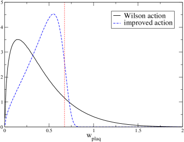
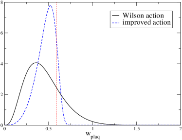
Figure 1: Histograms of the plaquette variable $w$ for the Wilson action and the improved action in the SU(2) and SU(3) case. The vertical lines show the corresponding effective cut $\gamma^{-1/q}$. The distributions were generated from simulations on $(L^{\prime}/a)^{4}=10^{4}$ volumes, where the lattice spacing was set to its coarsest value, defined by $L/a=4$ and $m_{100}(L)L=1.375$ and 1 for SU(2) and SU(3) respectively.

The optimization of the action is done by moving along the $\beta(\gamma)$ line to minimize the deviation of $u_{110}(L)\equiv m_{110}(L)L$ from its continuum limit. The latter was obtained by measuring the corresponding torelon masses at the same physical point $u_{100}(L)=u^{\star}$ and finer resolutions with the Wilson action and extrapolating to $a/L=0$. This way one obtains the pair of couplings ($\beta,\gamma$) which are optimal for this resolution (and the given choice of observables). One could proceed further on lattices with larger $L/a$, similarly to the case of the O($N$) spin model. Instead, we have chosen a less ambitious optimization: for finer resolutions we kept the same $\gamma$ as obtained on the coarse lattice $L/a=4$, and tuned only $\beta$ to obtain $u_{100}(L)=u^{\star}$ for $L/a=6$ and $8$. Then using these pairs of couplings ($\beta(a),\gamma$) we measured different quantities, like torelon masses on spatial lattices of different shapes, the static $q\overline{q}$ potential, and observables related to the gradient flow of the gauge fields.

It is worth to discuss briefly our choice of the basic physical quantity used for optimization. The torelon is an excitation characterized by an electric flux wrapping through the torus $L_{1}\times L_{2}\times L_{3}\times\infty$ in one (or several) periodic spatial directions. The Hilbert space of the transfer matrix is split into sectors characterized by quantum numbers $\mathbf{k}=(k_{1},k_{2},k_{3})$, where $k_{i}=0,\ldots,N-1$ for SU($N$). In particular, the value $k_{1}$ describes the transformation property of the corresponding state (the wave function in the strong-coupling basis) with respect to the multiplication by $z=\exp(2\pi i/N)$ of links $U_{1}(x_{1},x_{2},x_{3},t)$ at some plane with a given fixed $x_{1}$. Such a state can be created from a state in the vacuum sector $\mathbf{k}=(0,0,0)$ by multiplying it by a product of traces of Polyakov loops, or by the trace of a single Polyakov type loop wrapping around $(k_{1},k_{2},k_{3})$ times the spatial volume. We denote the trace of the Polyakov loop $\Phi_{i}$ in the direction $i$ on time slice $t$ by

$$\phi_{i}(t)=\mathrm{Tr}\,\Phi_{i}(t)\,,\quad i=1,2,3\,,$$ (2.3)

and

$$\phi_{\mathbf{k}}(t)=\phi_{1}(t)^{k_{1}}\phi_{2}(t)^{k_{2}}\phi_{3}(t)^{k_{3}}\,,\quad k_{i}=0,\ldots,N-1\,.$$ (2.4)

With this the torelon mass $m_{\mathbf{k}}=m_{\mathbf{k}}(L_{1},L_{2},L_{3})$ is obtained from the exponential fall-off of the correlation function

$$\langle\phi_{\mathbf{k}}(0)\phi_{\mathbf{k}}^{\dagger}(t)\rangle\sim A\exp(-m_{\mathbf{k}}t)\,.$$ (2.5)

The torelon mass (more precisely the energy difference between the lowest state in the sector characterized by electric flux $\mathbf{k}$ and the vacuum state) has a special dependence on the size and shape of the 3-volume. For small volumes $L\ll 1/T_{c}$ it is extremely small (it is given by a tunneling through a high barrier vanBaal ). In this case the flux is completely spread in the transverse direction. In a cubic 3-volume $L^{3}$ with increasing $L$ the flux assumes a finite width (“flux tube”) while its energy increases as $m_{100}(L)\sim\sigma L$, where $\sigma$ is the string tension. There is a relatively sharp transition between these two regimes, and we have chosen our physical lattice sizes (i.e. the value of $u^{\star}$) to be roughly in this region.

For asymmetric volumes $m_{100}(L_{1},L_{2},L_{3})$ increases with $L_{1}$, and decreases with increasing transverse sizes $L_{2}$, $L_{3}$. For $L_{1}=1/T_{c}$, $L_{2}=L_{3}=\infty$ the system undergoes a phase transition. We work here, however, in volumes where all spatial sizes $L_{i}$ are of $\mathcal{O}\left(1/T_{c}\right)$, hence the observables are smooth functions of $\beta$.

3 The SU(2) case

On a cubic spatial volume $L^{3}$ we define the fixed physical volume via the dimensionless combination $m_{100}L\equiv u_{100}(L)=u^{\star}=1.375$ i.e. the lattice size is measured in torelon mass units. At the chosen $u^{\star}$ value we measured the diagonal torelon state $u_{110}(L)$ on cubic spatial lattices of size $L/a=4,6,8,10$ using the Wilson action. The temporal extent $L_{t}$ was chosen to be either $10L$ or $20L$, the former corresponding to free boundary conditions in the time direction and the latter to periodic boundary conditions in the time direction. The advantage of free boundary conditions is that one can use a smaller lattice volume, with the drawback that time-like correlators can only be measured sufficiently far way from the ends. We used both setups to cross-check that they give consistent determinations of the torelon mass. The extrapolation to the continuum limit using a linear fit in $a^{2}$ gave $u_{110}(L)=2.888(5)$ (cf. figure 2).

To optimize the couplings in eq. (2.2) we tried first the choice $q=2$ on a $4^{3}\times 80$ lattice, but a more significant improvement of the cut-off effect has been found by increasing the power, and for the rest of our simulations we took $q=10$. Increasing $\gamma$ from the standard action case ($\gamma=0$) helps to decrease the cut-off effect for $u_{110}(L)$. We went up with this until $\gamma=52$, corresponding to an effective cut $\delta=\gamma^{-1/q}=0.67$ for $w$. At $L/a=4$ and $\gamma=52$ the condition

$$u_{100}(L)\equiv m_{100}(L)L=u^{\star}$$ (3.1)

yields $\beta=-2.4811$ (cf. table 1). Increasing $\gamma$ further – i.e. decreasing the effective constraint $\delta$ – lowers $\beta$, and the action density becomes restricted practically to a narrow region for $w$ closely below $\delta$. This would slow down significantly the effectiveness of the Monte Carlo simulations. We repeated the procedure for the improved action on $L/a=6$ and $8$, holding $q=10$ and $\gamma=52$ fixed.

The $u_{110}$ torelon masses measured using the standard Wilson action and separately the improved action are plotted in figure 2, together with the extrapolations to the continuum limit. The couplings of the actions are given in table 1, where we include an extrapolation from simulations to the chosen value of the physical point $u_{100}(L)=u^{\star}=1.375$. For the error propagation we used $du_{110}(L)/du_{100}(L)\approx 1.8$, measured by repeating the simulation at slightly different $\beta$.

In contrast to the situation with the O($N$) non-linear sigma model, for the SU($N$) case we could not completely eliminate the cut-off effects for the chosen pair of physical quantities, $u_{100}(L)$ and $u_{110}(L)$, on the coarsest $L/a=4$ lattice using the single-plaquette improved action with only one tunable parameter. However, the improved action significantly reduces the cut-off effect at $L/a=4$ down to 1%, compared to 6% for the Wilson action, and by $L/a=6$ the improved action result is essentially compatible with the continuum value. For both actions, the lattice artifacts appear to be ${\cal O}(a^{2})$ and we make our continuum extrapolations assuming quadratic dependence on the lattice spacing. We see very good agreement between the extrapolated values for the two lattice actions. We could make a more accurate determination for the continuum value of $u_{110}(L)$ with a constrained fit of Wilson and improved action data which demands that they have a common continuum limit, but that would not serve our purpose here to check for consistency between the two independent sets of simulations.

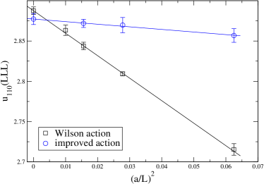
Figure 2: Cut-off effects of $u_{110}(L)$ on cubic lattices $L^{3}$ for the Wilson action and the improved action at $u_{100}(L)=1.375$ for SU(2).

9$L/a$	9999$\beta$	$\gamma$	$u_{100}(L)$	$u_{110}(L)$	$u_{110}^{\star}(L)$	$a$[fm]
4	2.29342	0.	1.3746(8)	2.7148(71)	2.7154(72)	0.175
6	2.42660	0.	1.3754(4)	2.8100(23)	2.8093(24)	0.112
8	2.51350	0.	1.3756(7)	2.8450(44)	2.8438(46)	0.082
10	2.58220	0.	1.3769(13)	2.8667(58)	2.8633(63)	0.064
4	$-2.4811$	52.	1.3737(16)	2.8544(81)	2.8568(85)
6	$-1.3720$	52.	1.3735(19)	2.8670(89)	2.8697(95)
8	$-0.7770$	52.	1.3730(13)	2.8683(46)	2.8719(51)

Table 1: Parameters of the SU(2) action and $u_{100}(L)$, $u_{110}(L)$ on cubic lattices at different lattice spacings, for the Wilson and the improved actions. The column $u_{110}^{\star}(L)$ is the value extrapolated to $u_{100}(L)=1.375$. For reference we include for the Wilson action the value of the lattice spacing as set via the string tension with $\sqrt{\sigma}=420$ MeV Lucini:2005vg .

3.1 Scaling Tests

Once the parameters of the action have been set as described above, we can proceed to examine the cut-off dependence of other physical quantities, to see what improvement the new action delivers. We start with a discussion of torelon masses measured on asymmetric spatial volumes.

We have measured the torelon masses on asymmetric spatial lattices both for the improved action and the standard Wilson action. Note that this is a completely independent set of lattice simulations from the ones which were used to tune the action parameters. We have considered shapes of type $(L,L,3L/2),(L,3L/2,3L/2),(L,L,2L)$ and $(L,2L,2L)$, with the shorthand notation $(LLr),(Lrr),(LLR)$ and $(LRR)$ in the plots and text. The corresponding results are shown in Figs. 3-5 for torelons which wrap around either one or two of the short spatial directions. One could also try to detect lattice artifacts in the heavier states such as the $u_{111}$ torelon in symmetric and asymmetric spatial volumes, but we found these masses could not be extracted with sufficient accuracy to be useful for comparison of cut-off dependence.

Let us first examine the $u_{100}$ states. As discussed earlier, the torelon wrapping around the shortest distance gets lighter as the transverse spatial directions increase in size. For example the $u_{100}(LRR)$ state is 2.5 times lighter than $u_{100}(L)=1.375$. This makes their determination from the exponential decay of Polyakov loop correlators somewhat easier, as the signal persists for larger time separation. We see that both for the improved and the Wilson actions the lattice artifacts again appear to be ${\cal O}(a^{2})$. Once extrapolated to the continuum, there is very good agreement between the two sets of simulations, except for some possible tension for $u_{100}(LRR)$. Note that there is no tuning done at this stage: the bare couplings $\beta$ and $\gamma$ have been fixed by requiring $u_{100}(L)=u^{\star}=1.375$. The improved action has consistently smaller lattice artifacts than the Wilson action, and on the coarsest lattice $L/a=4$, the cut-off dependence in e.g. the $u_{100}(LRR)$ is reduced from $\sim 25$% with the Wilson action to $\sim 4$% for the improved action.

We next discuss the $u_{110}$ states. An interesting empirical observation is that, while the $u_{100}$ masses approach the continuum limit from above, the $u_{110}$ masses approach it from below. Unfortunately, the statistical precision is not good enough to make a strong statement about reduced artifacts with the new action at finite lattice spacing. It is important however that we find consistency in the continuum results between the Wilson and improved action simulations, which are both determined with better than 1% precision.

Given that our tuning of the action parameters used $u_{100}(LLL)$ and $u_{110}(LLL)$, both measured on cubic $L^{3}$ spatial volumes, one of the limitations was the reduced statistical accuracy of the heavier $u_{110}$ state. An alternative strategy would be to fix the optimal couplings by choosing the pair $u_{100}(LLL)$ and $u_{100}(Lrr)$, the second state having a lighter mass and hence being easier to measure. However there is the drawback that one needs two full sets of simulations on both symmetric and asymmetric spatial lattices to complete the tuning. We pursued this approach and found the results were similar: with the new lattice action we could not completely eliminate the cut-off dependence on the coarsest $L/a=4$ lattice. Hence we do not show these results here.

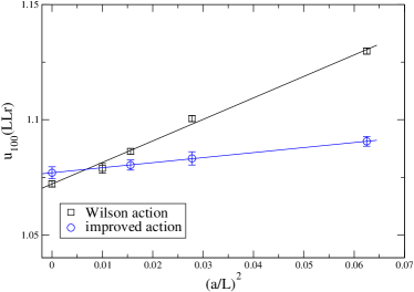
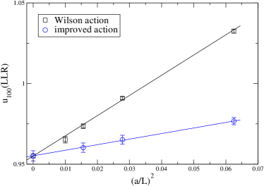
Figure 3: The $u_{100}$ torelon mass for SU(2) measured on spatial volumes (left) $(L,L,3L/2)$ and (right) $(L,L,2L)$.

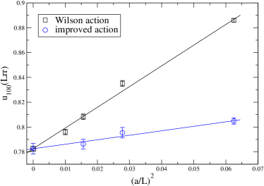
Figure 4: The $u_{100}$ torelon mass for SU(2) measured on spatial volumes (left) $(L,3L/2,3L/2)$ and (right) $(L,2L,2L)$.

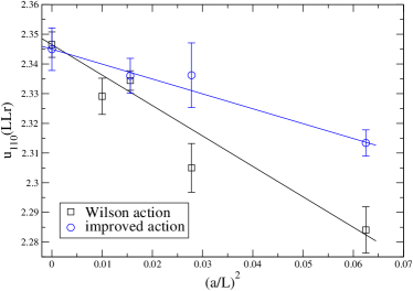
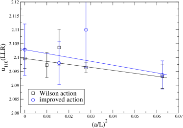
Figure 5: The $u_{110}$ torelon mass for SU(2) measured on spatial volumes (left) $(L,L,3L/2)$ and (right) $(L,L,2L)$.

At this point it is interesting to note that the SU(2) case is special. Considering a large spatial volume $L^{3}$, the flux tubes going along the diagonal directions, say along $(1,1,0)$ and $(1,-1,0)$ are obviously two different states. However, they belong to the same sector $\mathbf{k}=(1,1,0)$ in the SU(2) case. As a consequence, these states are mixed, and the eigenstates of the transfer matrix are even/odd w.r.t. $90^{\circ}$ rotation in the 1-2 plane. The operators producing these mass eigenstates from the vacuum sector can be constructed by

$$\phi_{110}^{(\pm)}(t)=\mathrm{Tr}\left(\Phi_{1}(t)\Phi_{2}(t)\pm\Phi_{1}(t)\Phi_{2}^{\dagger}(t)\right).$$ (3.2)

One expects that the energy difference between the odd and even lowest states is relatively large for small $L$ (where the width of the flux spreads over the available volume, and there is a large overlap between fluxes going along the two diagonals) and tiny for large $L$. Note that the operator given in (2.4) is an even one. Similar eigenstates also appear in the 111 sector. Although for some cases we measured the odd torelon masses like $m_{110}^{(-)}(L)$, we did not use them in this work.

3.2 Static Potential

In this section we present the scaling behavior of quantities related to the static potential. Usually the force between quarks is used as a practical and simple way to fix the scale, relating the bare coupling and the lattice spacing in physical units Sommer:1993ce . Here we consider the reverse approach. We investigate the approach to the continuum limit of the force between static quarks after fixing the scale with the torelon mass.

We have performed numerical simulations of SU(2) Yang-Mills theory comparing the standard Wilson action and the improved one. We have considered the bare couplings tuned with the torelon mass $m_{100}(L)$ for $L=4$, $6$ and $8$ and listed in table 1. The actual sizes of the simulated lattices were $24^{4}$, $36^{4}$ and $36^{3}\times 48$, respectively, for the three above parameter sets. The static potential has been measured on axis from the two-point correlation function of Polyakov loops at distance $r$

$$V(r)=-\frac{1}{L_{0}}\mbox{log}\langle\Phi(0)\Phi(r)\rangle$$ (3.3)

where $L_{0}$ is the lattice size along the temporal direction. The Monte Carlo simulations have been carried out using the multi-level algorithm Luscher:2001up . The force $F$ is obtained from the static potential by

$$F(r^{\prime})=V(r)-V(r-1)\,,$$ (3.4)

where $r^{\prime}$ is a properly chosen point between $r$ and $r-1$. The simplest case is the midpoint $r^{\prime}=r-1/2$. The cut-off effects can be somewhat reduced by choosing $r^{\prime}=r_{I}(r)$, the tree-level improved midpoint distance between $r$ and $(r-1)$ Sommer:1993ce . We present here the naive choice $r^{\prime}=r-1/2$, but the qualitative behavior of the cut-off effect is the same with the other choice as well.

The force is a dimensionful physical observable and it is useful to investigate its scaling behavior by considering the dimensionless quantity

$$H(r)=F(r)r^{2}.$$ (3.5)

We have studied the approach to the continuum limit of two scales, $r_{1}$ and $r_{2}$ defined as the distances where $H(r)$ has the values 1.0 and 1.65, respectively. Note that – as we mentioned above – one usually fixes the scale by defining the Sommer parameter, $r_{0}=0.5\,\mathrm{fm}$, as the distance where $H(r_{0})=1.65$. In figure 6 we show the scaling behavior of $r_{1}/L_{0}$ and $r_{2}/L_{0}$ as a function of $(a/L_{0})^{2}$ where the scale $L_{0}$ is defined by the torelon mass through $L_{0}m_{100}(L_{0})=1.375$. With the improved action, the reduction of lattice artifacts in the static force is less pronounced than in the torelon masses. For both actions the artifacts appear to be linear in $a^{2}$ and there is very good agreement between the continuum extrapolation results.

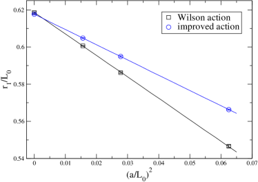
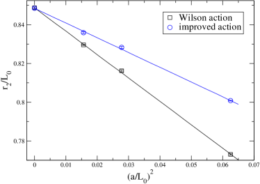
Figure 6: Approach to the continuum limit of $r_{1}/L_{0}$ (left) defined by $H(r_{1})=1$ and $r_{2}/L_{0}$ (right) defined by $H(r_{2})=1.65$ as a function of $(a/L_{0})^{2}$. $L_{0}$ is defined by $u_{100}(L_{0})=1.375$ .

It is important to note that the lattice artifacts of the static potential can be only partially attributed to the properties of the lattice action. The choice of the operator (say smeared Polyakov loops versus naive ones) also contributes, and it is not easy to separate these effects. Even in continuum electrostatics, the force between two charges of cubic shape is not exactly proportional to $1/r^{2}$, it also depends on the relative orientation of the cubes.

4 The SU(3) case

Due to its obvious relevance as part of QCD, and as a possible prelude for future work, we also tuned and tested the improved action in SU(3) gauge theory, and compared it to the standard Wilson action to see how much the cut-off effects could be suppressed. Because much of the procedure is similar to the SU(2) work described above, we avoid a detailed description of the common aspects.

We use the same parametrization of the gauge action as in eq. (2.2) and the same value $q=10$ to curb large fluctuations of the plaquette. For the tuning procedure, we again choose to keep the physical volume fixed in units of the torelon mass, with the precise value being $m_{100}(L)L\equiv u_{100}(L)=u_{100}^{\star}=1.0$. Note that for the same value of $L/a$ this corresponds to a somewhat finer lattice spacing than in our SU(2) study. Starting on the coarsest lattice $L/a=4$, we tested a range of values of $\gamma$, for each one finding the tuned coupling $\beta(\gamma)$ where the above condition was satisfied. We simultaneously measured the $u_{110}$ torelon mass at the same $\gamma$ and $\beta(\gamma)$ values. We found that for $\gamma=200$ the cut-off effects in the $u_{110}$ state were largely removed at this coarse lattice spacing. This corresponds to an effective cut on the plaquette values at $\delta=\gamma^{-1/q}=0.59$. Going to larger values of $\gamma$ significantly reduces the efficiency of the Monte Carlo simulations, with decreasing improvement in reducing lattice artifacts. For this reason, we used the fixed value $\gamma=200$ for the remainder of the SU(3) study.

$L/a$	9999$\beta$	$\gamma$	$u_{100}(L)$	$u_{110}(L)$	$u_{110}^{\star}(L)$	$a$[fm]
4	5.7299	0.	1.0000(11)	2.0990(32)	2.0990(37)	0.159
6	5.9806	0.	1.0000(9)	2.1797(28)	2.1797(33)	0.096
8	6.1749	0.	1.0000(25)	2.2050(53)	2.2050(74)	0.070
10	6.3364	0.	1.0000(36)	2.2066(100)	2.2066(126)	0.056
12	6.4741	0.	1.0000(35)	2.2141(110)	2.2141(130)	0.047
4	$-2.4104$	200.	1.0000(28)	2.1811(74)	2.1811(96)
6	0.2174	200.	1.0000(16)	2.1965(37)	2.1965(51)
8	1.4882	200.	1.0000(71)	2.2057(70)	2.2057(89)

Table 2: Parameters of the SU(3) action and $u_{100}(L)$, $u_{110}(L)$ on cubic lattices for the Wilson and the improved actions. The column $u_{110}^{\star}(L)$ includes in its error the propagated uncertainty in determining the location of $u_{100}(L)=1$. For reference we include for the Wilson action the value of the lattice spacing as set via the Sommer parameter $r_{0}=0.5$ fm Necco:2001xg .

We repeated the tuning exercise for the improved action at $L/a=6$ and 8, as well as finding the corresponding bare couplings for the Wilson action over a range of lattice sizes from $L/a=4$ to 12. Our procedure to tune the action parameters was technically slightly different for the SU(3) case. We measured simultaneously the torelon masses at $\sim 40$ nearby $\beta$ values, and fitted the $\beta$-dependence by a 5-th order polynomial. Then from these fits we determined the appropriate $\beta$ value from $u_{100}(L)=u^{\star}$ and used this to determine $u_{110}(L)$. The errors were determined by a bootstrap procedure. To present the data in a similar way as in table 1, in table 2 we give the value $u_{110}(L)$ corresponding to “fixed $\beta$” and $u^{\star}_{110}(L)$ corresponding to “fixed $u_{100}(L)=u^{\star}$”.

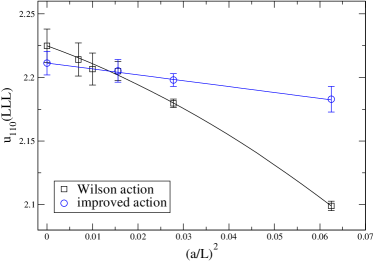
Figure 7: Cut-off effects of $u_{110}(L)$ on cubical lattices $L^{3}$ for the Wilson action and the improved action at $u_{100}(L)=1$ for SU(3).

We show the results for the $u_{110}(L)$ torelon mass for both improved and Wilson actions in figure 7. At the coarsest lattice spacing, the cut-off effects for the improved action are $\sim 1$% compared to $\sim 5$% for the Wilson action. Although both are small effects, at the level of accuracy we could reach they are clearly observable. Similar to SU(2), by $L/a=6$ the improved action measurement lies almost on top of the continuum extrapolated value. The overall smaller size of the cut-off effects compared to the SU(2) case is possibly due to the choice of a smaller value of $u_{100}^{\star}$. One contrast with respect to the SU(2) findings is that at this level of accuracy, the continuum extrapolation must be quadratic in $a^{2}$ for the Wilson action if one wishes to include the $L/a=4$ data point. For the improved action, an extrapolation linear in $a^{2}$ describes the data perfectly well.

4.1 Scaling Tests

As before for SU(2), once we complete the tuning procedure for $\gamma$ and $\beta(\gamma)$ on symmetric spatial volumes, we next move to asymmetric spatial volumes to examine what improvement the new action brings. The torelon mass results are shown in Figs. 8-10. The first question is whether or not there is good consistency between the continuum extrapolated results using the two lattice actions, to which the answer is yes. For the $u_{100}$ states the cut-off effects are largely suppressed on the coarsest $L/a=4$ lattice with the new action. For the Wilson action on $L\times L\times 2L$ and $L\times 2L\times 2L$ volumes, again the continuum extrapolation of the $u_{100}$ mass is quadratic in $a^{2}$ for the Wilson action, whereas the improved action extrapolation appears to be linear in $a^{2}$. The relative cut-off effect for the Wilson action increases as we go towards the largest spatial volume $L\times 2L\times 2L$, at which point the torelon is very light with $u_{100}(LRR)\approx 0.035$, given that the same state on a symmetric volume corresponds to $u_{100}=1$. The $u_{110}$ masses are determined with 1% accuracy or better, but as for SU(2), there is no clear reduction of lattice artifacts with the newly proposed action.

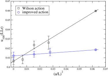
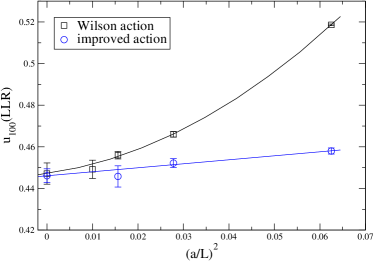
Figure 8: The $u_{100}$ torelon mass for SU(3) measured on spatial volumes (left) $(L,L,3L/2)$ and (right) $(L,L,2L)$.

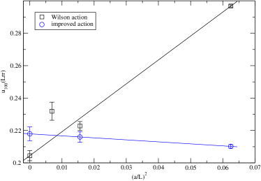
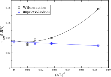
Figure 9: The $u_{100}$ torelon mass for SU(3) measured on spatial volumes (left) $(L,3L/2,3L/2)$ and (right) $(L,2L,2L)$.

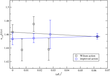
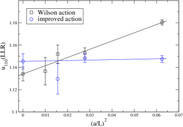
Figure 10: The $u_{110}$ torelon mass for SU(3) measured on spatial volumes (left) $(L,L,3L/2)$ and (right) $(L,L,2L)$.

To compare these lattice artifacts to those for the mixed fundamental-adjoint action we also measured the torelon masses for the action used in Hasenbusch:2004yq . Fixing the adjoint coupling to $\beta_{a}=-4.0$ as in Hasenbusch:2004yq , with the fundamental coupling $\beta_{f}=9.398$ for $L/a=4$ we obtained $u_{100}(L)=1.0036(8)$ and $u_{110}(L)=2.1502(27)$. This yields the extrapolated value $u_{110}^{\star}(L)=2.1435(31)$, which is halfway between values for the Wilson action and the newly proposed action (cf. table 2 and figure 7). Hence the mixed fundamental-adjoint action brings some improvement, but not as much as the new action we present.

4.2 Gradient flow observables

The gradient flow is a recently developed method which smooths out lattice fields in a controlled fashion and from which renormalized observables can be measured with very high accuracy Luscher:2010iy . In the following we make use of the fact that the gauge field obtained at flow time $t/a^{2}>0$ is a smooth renormalized field Luscher:2011bx . Hence, the expectation values of local gauge invariant expressions in this field are well-defined physical quantities that probe the theory at length scales on the order of $\sqrt{t}$. In particular, we will consider observables related to the action density $E(t)$ at flow time $t$, and the set of its derivatives

$$W^{(n)}(t)=(t\cdot\partial_{t})^{n}\left(t^{2}E(t)\right)\,.$$

One possible discretization of the action density on the lattice makes use of the sum of unoriented plaquettes with a common lower-left corner Luscher:2010iy and is denoted by $E_{\text{plaq}}(t)$, but we also used a more symmetric clover-type discretization $E_{\text{sym}}(t)$.

One way to exploit the gradient flow is to extract the lattice spacing. For example, one can define the lattice scale $\sqrt{t_{0}}$ via the requirement that

$$W^{(0)}_{0}\equiv\left.t^{2}\langle E(t)\rangle\right|_{t_{0}}=c,$$ (4.1)

where in the original investigation Luscher:2010iy the value $c=0.3$ was chosen. The corresponding value of $t_{0}/a^{2}$ can be measured with very good precision and be used as a reference scale when taking the continuum limit $a\rightarrow 0$. Similarly one can define a scale $w_{0}$ set by the requirement that

$$W^{(1)}_{0}\equiv\langle W^{(1)}(t)\rangle_{t=w_{0}^{2}}=c^{\prime},$$ (4.2)

where again there is freedom in the choice of the parameter $c^{\prime}$, which in the literature has first been tested for the choice $c^{\prime}=0.3$ Borsanyi:2012zs . Note that for a given choice of $c$ and $c^{\prime}$, the dimensionless ratio $t_{0}/w_{0}^{2}$ is physical and has a well-defined value in the continuum limit. Further derivatives of the action density renormalized at flow time $t_{0}$ can be determined by evaluating

$$W^{(n)}_{0}\equiv\langle W^{(n)}(t_{0},L)\rangle$$ (4.3)

and the continuum limit of these quantities is taken by $\lim_{a\rightarrow 0}W^{(n)}_{0}$.

Unlike the mass spectrum of the theory, gradient flow observables are not spectral quantities, therefore their cut-off dependence follows from (a) the lattice action used in the Monte Carlo generation of the ensembles, (b) the action used in implementing the flow, and (c) the lattice discretization of the action density. We generated separate ensembles using both the standard Wilson and improved lattice gauge actions over a range of lattice volumes and lattice spacings. For both sets, we use the Wilson action in the flow and we consider both $E_{\text{plaq}}$ and $E_{\text{sym}}$ to facilitate the continuum limit. It turns out that the gradient flow observables in lattice units are essentially independent of the volume above $L/\sqrt{t_{0}}\gtrsim 8.0-8.5$. As a consequence, we restricted our analysis of the results to simulations for which $L/\sqrt{t_{0}}>10.0$.

The quantification of the lattice artifacts due to the specific choice of the gradient flow action is beyond the scope of the present work, but the ones due to the discretization of the action density operator can be estimated by comparing the observables evaluated with $E_{\text{plaq}}$ and $E_{\text{sym}}$. In figure 11 we show the continuum limit of $W^{(0)}(t_{0})$ using the symmetrized definition for the action density while $t_{0}$ is determined from the plaquette definition. By construction $W^{(0)}(t_{0})$ takes the value $0.3$ in the continuum, independent of the discretization employed for the action density. The continuum limits displayed in figure 11 show that within two standard deviations this is indeed the case for our simulation results, both for the Wilson and the improved gauge action.

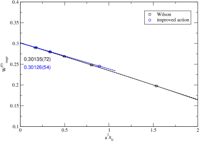
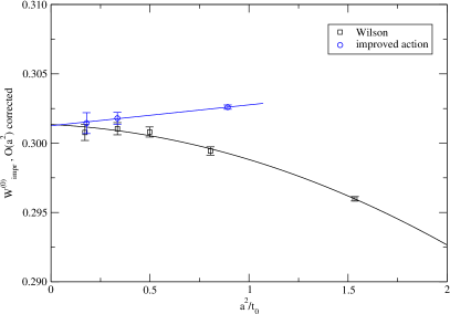
Figure 11: Continuum limit of $W^{(0)}(t_{0})$ using the symmetrized definition for the action density while $t_{0}$ is determined from the plaquette definition. Original data (left) and ${\cal O}(a^{2})$ corrected data (right).

In order to enhance the differences between the two actions, we removed the average ${\cal O}(a^{2})$ correction which one can assume stems from the discretization of the action density. We fit the results of the Wilson and improved action separately with an ansatz $c_{0}+c_{1}a^{2}+c_{2}a^{4}$, then average $c_{1}$ from both fits, and subtract $c_{1,ave}a^{2}$ from the original data. This is a convenient way to magnify the deviations. The result is displayed in the right plot of figure 11 and illustrates that the continuum extrapolations can be achieved by employing an ${\cal O}(a^{2})$ correction for the improved action, while ${\cal O}(a^{2})$ and ${\cal O}(a^{4})$ corrections are necessary for the Wilson action. However, it is clear that the differences between the results from the Wilson and the improved gauge action are very small. We assign this to the fact that the lattice artifacts introduced through the discretization of the operator and/or the choice of the flow procedure are so large that they dominate the ones due to the choice of the action for Monte Carlo simulation.

Yet another part of the challenge in quantifying the magnitude of cut-off effects is the ambiguity in the choice of lattice scale. To illustrate this, in figure 12 we consider the dimensionless ratio $t_{0}/w_{0}^{2}$ as a function of the lattice spacing expressed in units of $t_{0}$ (left plot) and in units of the torelon mass $m_{100}$ (right plot) determined earlier in the spectroscopy study. On the coarsest lattices, corresponding to $am_{100}=1/4$ for the new action, cut-off effects are now significantly smaller with the improved action. Still, the dominant effect at finite lattice spacing is the choice of the action density operator. We tried to separate out the effect of the operator by considering a linear combination of $E_{\text{plaq}}$ and $E_{\text{sym}}$, so as to reduce the lattice artifacts stemming from the discretization of the action density operator. However, even in the improved combination the difference between the standard and new lattice actions is not dramatic.

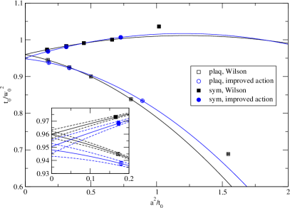
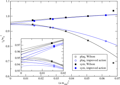
Figure 12: Continuum limit of the dimensionless ratio $t_{0}/w_{0}^{2}$ using the plaquette and the symmetrized definition for the action density in terms of $a^{2}/t_{0}$ (left plot) and in terms of $(am_{100})^{2}$ (right plot).

Given the high precision of the gradient flow method, it is interesting to investigate how many derivatives of the action density can be accurately measured. In figure 13 we show the continuum limit of the first and second derivatives of the action density calculated from both the plaquette and symmetrized definition, and for both gauge actions, with $t_{0}$ always being determined from the corresponding definition. We see that lattice artifacts remain large and are again dominated by the choice of operator, not the lattice action used to generate the ensemble. Most important, we see consistent continuum results across the various discretizations, and cut-off effects which are always well described by ${\cal O}(a^{2})$ and ${\cal O}(a^{4})$ corrections.

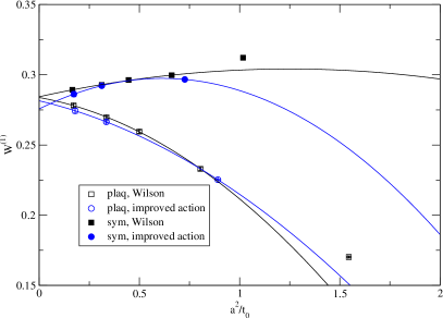
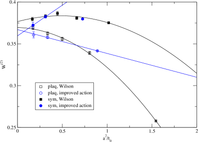
Figure 13: Continuum limit of the dimensionless derivatives $W^{(1)}(t_{0})$ and $W^{(2)}(t_{0})$ using the plaquette and the symmetrized definition for the action density.

4.3 Plaquette distribution

To investigate further the origin of cut-off effects in observables related to the gradient flow, we studied the distribution of the plaquette and its evolution along the flow. This is shown in figures 14-16. The plaquette distribution on the original gauge configurations generated during the Monte Carlo simulation are very different, by design: the new action essentially suppresses large fluctuations, with the peak occurring further from the limiting value where the plaquette is unity. As we tune to finer lattice spacing, the distributions move smoothly. If we inspect the plaquette distributions at flow time $t_{0}$ in figures 15 and 16, a different picture emerges. The Wilson and improved action ensembles have very similar distributions once the coarse fluctuations are smoothened out, with a rapidly decreasing tail of plaquette values away from 1. Using higher resolution to probe the region closest to 1, we see again the strong similarity between the ensembles. The gradient flow washes out lattice artifacts contained in the original lattice action, which are replaced by discretization effects of the flow scheme instead. Obviously, the matching of the distributions between the two actions is in line with matching the lattice spacings from the gradient flow, and this is the reason why the gradient flow observables from the two actions show rather similar lattice artifacts.

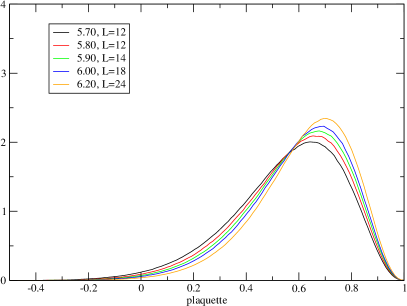
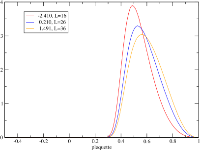
Figure 14: Distribution of the plaquette values of the original gauge field configurations. The left panel corresponds to the Wilson ensembles while the right panel shows the improved action ensembles.

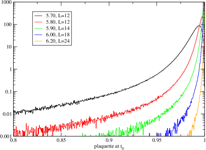
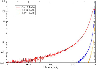
Figure 15: Distribution of the plaquette values of the gauge field configurations at flow time $t_{0}$. The left panel corresponds to the Wilson ensembles while the right panel shows the improved action ensembles, both at flow time $t_{0}$.

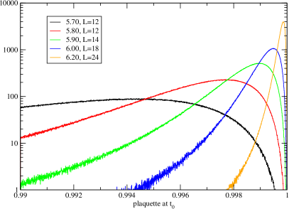
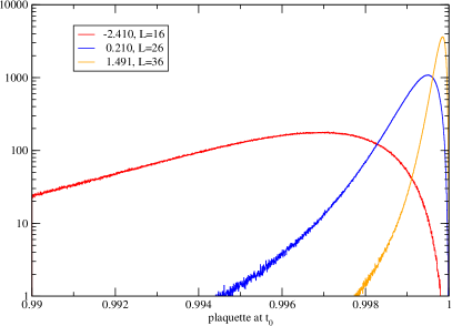
Figure 16: Magnification of the distribution of the plaquette values of the gauge field configurations. Left plot for Wilson ensembles, right plot for improved action ensembles at flow time $t_{0}$.

5 Algorithms and Cost Estimates

The obvious drawback to using an improved action in lattice simulations is the increased numerical cost, both in construction and in the Monte Carlo simulation, where smaller updates are needed for e.g. the Metropolis algorithm to have a reasonable acceptance rate. Hence an increased time is necessary in reaching a given numerical accuracy for a fixed computational resource. This has to be balanced against the expectation of being able to determine continuum results using coarser lattices than for the standard action. The motivation to examine a new action as parametrized in eq. (2.2) is that using only powers of the basic plaquette minimizes the numerical cost, while the suppression of large plaquette fluctuations is achieved in a way very different than for lattice actions constructed along the Symanzik improvement program.

Let us consider the numerical slowdown. For one sweep of a lattice volume, the CPU time taken for the improved action relative to the Wilson action is $t_{\rm imp}/t_{\rm Wil}=1.9$, both for SU(2) and SU(3) gauge theory. In order to estimate the autocorrelation time, we compare the squared relative error of the Polyakov loop correlator at distance $t=L$, normalized to the same number of sweeps, $(\Delta C(t)/C(t))^{2}\times n_{\rm sweep}$, which we found for SU(3) is 1.4 times larger with the improved action than for the Wilson action (for an acceptence rate $\sim 0.5$ for both actions). For a different determination of the autocorrelation time, we also examined the torelon mass error, also normalized to the same number of sweeps, $(\Delta m)^{2}\times n_{\rm sweep}$. For this quantity we find an increase by a factor of 1.5 going from the standard to the new action, essentially the same value. Hence to achieve a given statistical accuracy our new action is about 3 times more expensive in computer time than the Wilson action. However, the reduction in cut-off effects more than compensates for the increased cost. As a rough estimate, taking into account that the $a^{2}$ cut-off effect is reduced by a factor $\sim 5$, to reach the same cut-off error and statistical error one gains in computer time a factor $5^{3}/3\approx 40$, assuming the CPU time needed for an independent configuration grows like $(L/a)^{6}$ (lattice volume $\times$ critical slowing down). We can only speculate that for full QCD the gain could be even larger.

We use two different algorithms for Monte Carlo simulations with the improved action. One is a standard Metropolis update, where a trial gauge link is generated by a rotation of the original gauge link, followed by an accept/reject decision. The rotation has an adjustable parameter, which allows one to tune to whatever desired acceptance rate. A different algorithm is where a trial gauge link is generated using the standard heathbath algorithm for the Wilson action, but with a bare coupling $\beta^{\prime}\neq\beta$. The trial gauge link is then accepted or rejected with a Metropolis step based on the change of the action $(\beta-\beta^{\prime})w+\gamma w^{q}$. The adjustable parameter here is $\beta^{\prime}$ which can be tuned to improve the acceptance rate, however the rate cannot be made arbitrarily close to 100%. We find similar efficiency between the two algorithms in our Monte Carlo results.

6 Conclusions

The type of lattice action we propose and study in this paper is somewhat unusual, given that it does not have the usual naive continuum limit. On the basis of universality, the essential elements are the dimensionality of the system and that the lattice action has the correct internal symmetries. Our numerical results fully support this view and show beyond any doubt that our chosen discretization gives the correct continuum theory.

The findings regarding suppression of lattice artifacts depend on the observable in question. In the case of spectral quantities such as the torelon masses it was possible to almost fully remove cut-off dependence on the coarsest lattice we simulate. For non-spectral quantities such as the static quark potential and force, and observables given by the gradient flow such as the lattice scales $t_{0}$ and $w_{0}$, improvement in the operators is necessary beyond just improvement of the action, as can be seen from the reduction but not the removal of artifacts. We did not measure other spectral quantities such as the glueball spectrum, the critical temperature $T_{c}$ and the string tension $\sigma$, since those studies would require larger numerical simulations. The tuning strategy we choose is based on the torelon spectrum. The parametrization is general – one could extend it without increasing the numerical cost by adding an adjoint plaquette term to the action, which opens up the possibility that additional tuning of the extra parameters would give even further reduction of lattice artifacts.

Our study of the gradient flow and its use in scale setting, as well as observables given by higher order derivatives of the renormalized action density, is a useful test of the accuracy of the scheme and of the systematics due to lattice artifacts, as well as a test for universality.

The newly proposed lattice action is cheap and would be straightforward to incorporate into simulations with dynamical fermions. The crucial question is how much of the improvement carries over to such simulations, which remains to be investigated.

7 Acknowledgments

The research leading to these results has received funding from the Schweizerischer Nationalfonds and from the European Research Council under the European Union’s Seventh Framework Programme (FP7/2007-2013)/ ERC grant agreement 339220. We also acknowledge support by the US National Science Foundation under the grants NSF 0970137 and 1318220. KH wishes to thank the Institute for Theoretical Physics and the Albert Einstein Center for Fundamental Physics at the University of Bern for their support.

References

- (1) K. Symanzik, Nucl. Phys. B 226, 187 (1983).
- (2) K. Symanzik, Nucl. Phys. B 226, 205 (1983).
- (3) M. Lüscher and P. Weisz, Commun. Math. Phys. 97, 59 (1985).
- (4) M. Lüscher and P. Weisz, Phys. Lett. B 158, 250 (1985).
- (5) P. Hasenfratz and F. Niedermayer, Nucl. Phys. B 414, 785 (1994) [hep-lat/9308004].
- (6) W. Bietenholz and U.-J. Wiese, Nucl. Phys. B 464, 319 (1996) [hep-lat/9510026].
- (7) F. Niedermayer, P. Rüfenacht and U. Wenger, Nucl. Phys. B 597, 413 (2001) [hep-lat/0007007].
- (8) P. Hasenfratz, S. Hauswirth, T. Jörg, F. Niedermayer and K. Holland, Nucl. Phys. B 643, 280 (2002) [hep-lat/0205010].
- (9) C. Gattringer et al. [Bern-Graz-Regensburg Collaboration], Nucl. Phys. B 677, 3 (2004) [hep-lat/0307013].
- (10) R. W. B. Ardill, K. J. M. Moriarty and M. Creutz, Comput. Phys. Commun. 29, 97 (1983).
- (11) T. Blum, C. E. DeTar, U. M. Heller, L. Karkkainen, K. Rummukainen and D. Toussaint, Nucl. Phys. B 442, 301 (1995) [hep-lat/9412038].
- (12) U. M. Heller, Phys. Lett. B 362, 123 (1995) [hep-lat/9508009].
- (13) M. Hasenbusch and S. Necco, JHEP 0408, 005 (2004) [hep-lat/0405012].
- (14) W. Bietenholz, K. Jansen, K.-I. Nagai, S. Necco, L. Scorzato and S. Shcheredin, JHEP 0603 (2006) 017 [hep-lat/0511016].
- (15) H. Fukaya, S. Hashimoto, T. Hirohashi, K. Ogawa and T. Onogi, Phys. Rev. D 73 (2006) 014503 [hep-lat/0510116].
- (16) M. Lüscher, Nucl. Phys. B 549 (1999) 295 [hep-lat/9811032].
- (17) M. Hasenbusch, P. Hasenfratz, F. Niedermayer, B. Seefeld and U. Wolff, Nucl. Phys. Proc. Suppl. 106, 911 (2002) [hep-lat/0110202].
- (18) F. Knechtli, B. Leder and U. Wolff, Nucl. Phys. B 726, 421 (2005) [hep-lat/0506010].
- (19) J. Balog, F. Niedermayer and P. Weisz, Phys. Lett. B 676, 188 (2009) [arXiv:0901.4033 [hep-lat]].
- (20) J. Balog, F. Niedermayer and P. Weisz, Nucl. Phys. B 824, 563 (2010) [arXiv:0905.1730 [hep-lat]].
- (21) M. Bögli, F. Niedermayer, M. Pepe and U.-J. Wiese, JHEP 1204, 117 (2012) [arXiv:1112.1873 [hep-lat]].
- (22) W. Bietenholz, U. Gerber, M. Pepe and U.-J. Wiese, JHEP 1012, 020 (2010) [arXiv:1009.2146 [hep-lat]].
- (23) J. Balog, private communication.
- (24) P. de Forcrand, M. Pepe and U.-J. Wiese, Phys. Rev. D 86, 075006 (2012) [arXiv:1204.4913 [hep-lat]].
- (25) J. Balog, F. Niedermayer, M. Pepe, P. Weisz and U.-J. Wiese, JHEP 1211, 140 (2012) [arXiv:1208.6232 [hep-lat]].
- (26) O. Akerlund and P. de Forcrand, JHEP 1506, 183 (2015), [arXiv:1505.02666 [hep-lat]].
- (27) M. Lüscher, P. Weisz and U. Wolff, Nucl. Phys. B 359, 221 (1991).
- (28) M. Lüscher, Phys. Lett. B 118, 391 (1982).
- (29) R. Sommer, Nucl. Phys. B 411, 839 (1994) [hep-lat/9310022].
- (30) M. Lüscher and P. Weisz, JHEP 0109, 010 (2001) [hep-lat/0108014].
- (31) G. ’t Hooft, Nucl. Phys. B 153, 141 (1979).
- (32) P. van Baal, Nucl. Phys. B 264, 548 (1986).
- (33) B. Lucini, M. Teper and U. Wenger, JHEP 0502, 033 (2005) [hep-lat/0502003].
- (34) S. Necco and R. Sommer, Nucl. Phys. B 622, 328 (2002) [hep-lat/0108008].
- (35) M. Lüscher, JHEP 1008, 071 (2010) [JHEP 1403, 092 (2014)] [arXiv:1006.4518 [hep-lat]].
- (36) M. Lüscher and P. Weisz, JHEP 02, 051 (2011) [arXiv:1101.0963 [hep-ph]].
- (37) S. Borsanyi, S. Dürr, Z. Fodor, C. Hoelbling, S. D. Katz, S. Krieg, T. Kurth and L. Lellouch et al., JHEP 1209, 010 (2012) [arXiv:1203.4469 [hep-lat]].