Likelihood of Cyber Data Injection Attacks to Power Systems

Abstract

Cyber data attacks are the worst-case interacting bad data to power system state estimation and cannot be detected by existing bad data detectors. In this paper, we for the first time analyze the likelihood of cyber data attacks by characterizing the actions of a malicious intruder. We propose to use Markov decision process to model an intruder’s strategy, where the objective is to maximize the cumulative reward across time. Linear programming method is employed to find the optimal attack policy from the intruder’s perspective. Numerical experiments are conducted to study the intruder’s attack strategy in test power systems.

I Introduction

State estimation [1] solves for power system states from obtained measurements. The correct estimation of systems states is vital for the reliable operation of power systems. Since bad data can result in significant errors in the outcome of state estimation and potentially lead to catastrophic consequences, the detection and identification of bad data has been extensively studied [3, 6, 14, 13, 21] in state estimation.

The integration of cyber infrastructures in future smart grids inevitably increases the possibility of cyber attacks. Cyber data attacks, firstly studied in [12], means that a malicious intruder with system configuration information simultaneously manipulates multiple measurements and the injected errors cannot be detected by any bad data detector.

State estimation in the presence of cyber data attacks has attracted much research attention recently [2, 4, 9, 11, 12, 17, 16, 18]. Some work focused on the identification of a small number of key measurement units such that if those units are protected from an intruder, the intruder cannot launch a successful cyber data attack [2, 4, 8]. A few recent work [17, 11, 19] considered the detection of cyber data attacks in a power system with Supervisory Control and Data Acquisition (SCADA) systems or phasor measurement units (PMUs) and various detection methods have been proposed.

What is missing in the literature of cyber data attacks is the analysis of the frequency of data attacks in smart grids and the likelihood of attacks at a given system state. This paper takes the first step to analyze the likelihood of data attacks from the intruder’s perspective. We consider a scenario that if a cyber data attack is detected by the operator, the affected measurement units will be protected for some time. Thus, the intruder’s current action affects its future available actions. To address such challenge in developing an attack strategy, we propose to use Markov Decision Process (MDP) [15] to model the intruder’s attack decision across time. The solution to the resulting MDP is a mapping from system states to the intruder’s actions (attack or not, which bus to attack and how much error to inject). Numerical experiments are carried on PJM 5-bus system to verify the proposed approach and study the likelihood of cyber attacks in such systems.

The rest of the paper is organized as follows. We motivate the problem and introduce cyber data attacks and MDP in Section II. We formulate the intruder’s attack strategy as an MDP and introduce its solution method in Section III. Section IV records our numerical study on an example network. We conclude the paper in Section V.

II Problem Motivation and Background

We first introduce the definition and existing work on cyber data attacks in Section II-A. We then motivate and introduce the problem of likelihood analysis of cyber data attacks in Section II-B. One main contribution of our paper is to model this problem as a Markov Decision Process (MDP). MDPs are introduced in Section II-C.

II-A Cyber Data Attacks in Power Systems

In a power system, the state is usually represented by bus voltage magnitudes $\bm{V}\in\mathcal{R}^{n}$ and angles $\bm{\theta}\in[-\pi,\pi]^{n}$, where $n$ is the number of buses. State estimation [1] solves for system states from the obtained measurements. Under the AC measurement model, the measurements $\bm{z}$ can be expressed as a nonlinear function of state variables $\bm{x}=(\bm{V}$,$\bm{\theta}$):

$$\bm{z}=h(\bm{x})+\bm{\omega},$$ (1)

where $\bm{\omega}$ represents the random measurement noise.

In the AC state estimation, the state variables are determined from the weighted least square optimization problem:

$$\bm{\hat{x}}=\arg\min(\bm{z}-h(\bm{x}))^{T}\cdot\bm{R}^{-1}\cdot(\bm{z}-h(\bm{x})),$$ (2)

where $\bm{R}$ is the covariance matrix of measurement noise $\bm{\omega}$.

Malicious intruders can hack the measuring devices and inject interacting errors to the measurements. If they have sufficient system information and choose the errors $\bm{e_{z}}$ satisfying

$$\begin{split}\bm{z}+\bm{e_{z}}&=h(\bm{x^{\prime}})+\bm{\omega}\\ &=h(\bm{V}+\bm{e_{V}},\bm{\theta}+\bm{e_{\theta}})+\bm{\omega},\end{split}$$ (3)

where $\bm{e_{V}}$ and $\bm{e_{\theta}}$ represent the resulting errors on state variables $\bm{V}$ and $\bm{\theta}$ respectively, the manipulated measurements cannot be detected by existing bad data detectors. In this case, instead of correctly estimating state variables ($\bm{V},\bm{\theta}$), the operator would obtain a wrong estimate $(\bm{V}+\bm{e_{V}},\bm{\theta}+\bm{e_{\theta}})$.

Since such cyber data attacks cannot be identified by bad data detectors, many efforts have been devoted to identify and protect a small number of key measurement units such that an intruder cannot inject unobservable attacks without hacking protected units [2, 4, 8]. A few recent work [17, 11, 19] considered the detection of data attacks and various detection methods have been proposed.

The potential financial risks of cyber data attacks are studied in [20] and [7], where the congestion pattern is defined as the set of congested lines. By injecting false data without being detected, the intruders could change the congestion pattern and thus change the locational marginal price (LMP). The intruders can obtain financial reward from the resulting change in LMP.

In this paper, we restrict our attention to attacks that satisfy (3) and result in a change of the system congestion pattern. By launching a data attack, if a line’s real power is wrongly estimated to exceed its capacity while it actually is not, or the power is wrongly estimated to below its limit while the line is actually congested, then the intruder can gain a reward from the attack.

II-B Likelihood of Cyber Data Attacks

One important question that has not been considered before is the analysis of the likelihood of cyber data attacks at a given operating state of power systems.

In this paper, we act as an intruder and aim to find the optimal attack strategy from an intruder’s perspective. We assume that an intruder can obtain a reward from a change of the congestion pattern by injecting false data without being detected. The intruder aims to maximize the cumulative reward. If a cyber data attack, however, is detected by detection methods such as [17, 11, 19], we assume the intruded measuring devices will be protected for some time so that an intruder cannot change the measurements of these devices during the period. A detected attack, therefore, can limit the intruder’s future actions and thus reduce the future reward. Since the state of a power system changes across time, and the future state is unknown to the intruder, it needs to decide when and which buses to attack to maximize the total rewards based on its current estimate. We employ Markov Chains [15] to model the evolution of power system states and formulate the intruder’s decision process as a Markov Decision Process [15]. The solution of resulting MDP is a mapping from system states to the intruder’s actions.

II-C Markov Decision Processes (MDPs)

An MDP is a mathematical framework employed to model the decision-making process in stochastic environments. In this framework, the system is modeled via a series of states $S$. Each state $s\in S$ has an associated set of actions $A(s)$. In time step $t$, a decision is made based on the system’s current state $s_{t}\in S$, and an action $a_{t}\in A(s_{t})$ is chosen to conduct. The cost of taking action $a_{t}$ at state $s_{t}$ is $G(s_{t},a_{t})$. Then following the state transition probability distribution, the system transits to a new state $s_{t+1}$ with a probability of $P(s_{t+1}|s_{t},a_{t})$. A reward $R(s_{t+1}|s_{t},a_{t})$ is received from the state transition. As the system evolves, a sequence of rewards is obtained. The aim for decision-makers is to choose sequential actions that yield maximal expected rewards over the total decision-making horizon. The MDP problem can be solved by numerous methods, like value iteration, policy iteration and linear programming approaches discussed in [15].

III Problem Formulation and Solution

In Section III-A, the problem is formulated from the perspective of attackers and the strategy of cyber data attacks is modeled as an infinite-horizon MDP. The solution method of resulting MDP is discussed in Section III-B.

III-A Problem Formulation

III-A1 States and Time Steps

Here we employ bus voltage magnitudes, angles and the states of measuring devices together as system states in an MDP. Because the measurements contain noise and an intruder may have limited knowledge of the states of a power system, we use discrete states to model the intruder’s estimate of actual power system states. For example, let $V_{i}$ denote the voltage magnitude of bus $i$, $V_{i}^{\max}$ and $V_{i}^{\min}$ denote the upper bound and lower bound of $V_{i}$ respectively. $\Delta V_{i}=V_{i}^{\max}-V_{i}^{\min}$. $n_{V}$ denotes the number of discrete states in the range. We define the state of the voltage magnitude of bus $i$ as

$$\bar{V}_{i}=q/(n_{V}-1),\ q\in\{0,1,\cdots,n_{V}-1\},$$ (4)

if $V_{i}\in\left[V_{i}^{\min}+q\times\tfrac{\Delta V_{i}}{n_{V}-1},V_{i}^{\min}+(q+1)\times\tfrac{\Delta V_{i}}{n_{V}-1}\right)$. Similarly, let $\theta_{i}$ denote the voltage angle of bus $i$, $\theta_{i}^{\max}$ and $\theta_{i}^{\min}$ denote its upper bound and lower bound respectively, $n_{\theta}$ denote the number of discrete states. $\Delta\theta_{i}=\theta_{i}^{\max}-\theta_{i}^{\min}$. We say the state of the voltage angle of bus $i$ is

$$\bar{\theta}_{i}=q/(n_{\theta}-1),\ q\in\{0,1,\cdots,n_{\theta}-1\},$$ (5)

if $\theta_{i}\in\left[\theta_{i}^{\min}+q\times\tfrac{\Delta\theta_{i}}{n_{\theta}-1},\theta_{i}^{\min}+(q+1)\times\tfrac{\Delta\theta_{i}}{n_{\theta}-1}\right)$. The state of the $j$th measuring device is denoted by a variable $\bar{U}_{j}$:

$$\bar{U}_{j}=\begin{cases}1&\text{$j$th device is open to attack},\\ 0&\text{$j$th device is protected from intrusion }.\end{cases}$$ (6)

If a measuring device is protected, then an intruder cannot change any measurements of that device. Otherwise, an intruder can change partial or all measurements of that device.

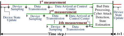
Figure 1: Event sequence with cyber data attacks. An intruder changes the observations of measuring devices to mislead the operator.

We consider a discrete-time system, and the time step is set as the duration between two consecutive instants of state estimation. The sampling rate of measuring devices can be higher than the state estimation frequency, as shown in Fig. 1. Attacks can happen during either device sampling or data transmission to control center. We assume if intruders decide to attack a device during step $t$, they need to change all the measurements of that device in the time step. Otherwise, the attack can be easily detected by comparing consecutive measurements. If a power system has $M$ buses and $N$ devices, the state $s_{t}$ at time step $t$ is

$$\begin{split}s_{t}&=\left[\bar{\bm{V}}(t),\bar{\bm{\theta}}(t),\bar{\bm{U}}(t)\right]\\ &=\left[\bar{V}_{1}(t),\cdots,\bar{V}_{M}(t),\bar{\theta}_{1}(t),\cdots,\bar{\theta}_{M}(t),\bar{U}_{1}(t),\cdots,\bar{U}_{N}(t)\right],\end{split}$$ (7)

where $\bar{V}_{i}(t)$, $\bar{\theta}_{i}(t)$ and $\bar{U}_{j}(t)$ represent the states of voltage magnitude and angle of bus $i$ and the state of $j$th device at time step $t$ respectively.

III-A2 Actions, Rewards and Costs

Since the reward results from a change in the congestion pattern, in order to change the line power, the intruder needs to inject errors to the estimate of voltage phasors of incident buses. Let $e_{V_{i}}$ and $e_{\theta_{i}}$ denote the injected errors to the voltage magnitude and angle of bus $i$ respectively. To make the problem tractable, we assume $e_{V_{i}}$ and $e_{\theta_{i}}$ can only be multiples of $\frac{\Delta V_{i}}{n_{V}-1}$ and $\frac{\Delta\theta_{i}}{n_{\theta}-1}$ respectively, and the resulting estimates of system variables still lie in individual allowable range. In this case, there are totally $n_{V}\times n_{\theta}$ available ways to inject errors to one bus voltage phasor. Note that in order to pass the bad data detection, given $\bm{e_{V}}$ and $\bm{e_{\theta}}$, an intruder needs to choose the injected errors $\bm{e_{z}}$ to measurements according to (3).

We call a set of buses and lines as target buses and target lines respectively if the intruder attempts to change the congestion pattern of these lines by injecting errors on the target buses. Since an intruder may have limited resources to launch attacks, we assume at each time step the intruder can manipulate the states of at most $d$ bus voltages. The intruder, therefore, has at most $\sum_{i=0}^{d}\tbinom{M}{i}$ ways to select target buses.

The launched attacks can be detected by some recently developed methods, as presented in section II-B. Here we use $p_{d}(s,a)$ to denote the probability that an action $a$ at state $s$ is detected by the network operator. We suppose it is a function of injected errors on the bus voltage magnitudes and angles:

$$p_{d}(s,a)=1-\exp\left(-C\times\sum_{i=1}^{M}\left(\frac{|e_{V_{i}}|}{\Delta V_{i}}+\frac{|e_{\theta_{i}}|}{\Delta\theta_{i}}\right)\right),$$ (8)

where $C$ is a positive constant. Intuitively, a larger $C$ means a higher probability with which the launched attack can be detected.

Since the bus voltage magnitudes and angles are in discretized states, instead of computing the power flow of line $ij$ directly from one specific state $(\bar{\bm{V}},\bar{\bm{\theta}})$, we can obtain the lower and upper bound of its absolute value, denoted as $P_{ij}^{\min}(\bar{\bm{V}},\bar{\bm{\theta}})$ and $P_{ij}^{\max}(\bar{\bm{V}},\bar{\bm{\theta}})$ respectively. Since the reward results from a change in the congestion pattern, we define the reward as a function proportional to the gap between the line’s flow limit and the power bounds with injected errors:

$$R_{ij}=\begin{cases}K_{ij}\times\left(P_{ij}^{\min}(\bar{\bm{V^{\prime}}},\bar{\bm{\theta^{\prime}}})-P_{ij}^{\text{M}}\right)/P_{ij}^{\text{M}},\\ \text{if}\enspace P_{ij}^{\min}(\bar{\bm{V^{\prime}}},\bar{\bm{\theta^{\prime}}})>P_{ij}^{\text{M}}>P_{ij}^{\max}(\bar{\bm{V}},\bar{\bm{\theta}});\\ K_{ij}\times\left(P_{ij}^{\text{M}}-P_{ij}^{\max}(\bar{\bm{V^{\prime}}},\bar{\bm{\theta^{\prime}}})\right)/P_{ij}^{\text{M}},\\ \text{if}\enspace P_{ij}^{\min}(\bar{\bm{V}},\bar{\bm{\theta}})>P_{ij}^{\text{M}}>P_{ij}^{\max}(\bar{\bm{V^{\prime}}},\bar{\bm{\theta^{\prime}}}).\end{cases}$$ (9)

where $K_{ij}$ is the given reward weight of line $ij$, $P_{ij}^{\text{M}}$ is the power flow limit of line $ij$, $(\bar{\bm{V^{\prime}}},\bar{\bm{\theta^{\prime}}})$ is the resulting estimate of system states by injecting errors $(\bm{e_{V}},\bm{e_{\theta}})$ to $(\bar{\bm{V}},\bar{\bm{\theta}})$.

The expected immediate reward from action $a$ at state $s$ is:

$$\begin{split}R(s,a)&=\sum_{s^{\prime}}P(s^{\prime}|s,a)\times R(s^{\prime}|s,a)\\ &=(1-p_{d}(s,a))\times\sum_{ij\in\Phi(s,a)}R_{ij}.\end{split}$$ (10)

where $\Phi(s,a)$ is the set of target lines.

We assume the cost to intrude an accessible measuring device is fixed and known to an intruder, denoted by $g_{u}$. Let $f(\Phi(s,a))$ denote the number of intruded measuring devices in attack $a$, the attack cost at state $s$ is:

$$G(s,a)=g_{u}\times f(\Phi(s,a)).$$ (11)

III-A3 State Transition Probabilities

We assume all measuring devices that are currently open to attack will stay open without attack. An action $a$ at state $s$ is detected with probability $p_{d}(s,a)$, and the intruded devices will be protected as a whole in the next time step. Each protected device will change to open in the next time step with a fixed probability $p_{T}$. Intuitively, a smaller $p_{T}$ indicates that once protected, a device is more likely to stay inaccessible to intruders for a longer period of time. When $p_{T}=0$, it means the protected devices will no longer be accessible to intruders.

To model the dynamics of a power system, we assume each load in the system evolves independently as a Markov Chain [15] and the system state is determined from economic dispatch. We assume each load has $n_{L}$ states and a load can transit from state $q_{1}$ to state $q_{2}$ with a fixed and known probability $p_{q_{1},q_{2}}$. In practice, one can learn these transition probabilities from historical data. In this case, in a power network with $M$ buses and $N$ devices, if $M_{L}$ loads evolve as Markov Chains, the total number of system state is $n_{L}^{M_{L}}\times 2^{N}$.

III-B MDP Solutions

A linear programming approach [5, 15] is applied to solve MDP. A stationary policy $\pi$ for an MDP is a mapping $\pi:S\mapsto A$, where $\pi(s)$ is the action taken in state $s$. We define $W_{\pi}(s)$ as the cumulative expected net reward by starting from state $s$ and following policy $\pi$,

$$W_{\pi}(s)=E\left[\sum_{t=0}^{\infty}\gamma^{t}\left(R(s_{t},\pi(s_{t}))-G(s_{t},\pi(s_{t}))|s_{0}=s\right)\right],$$ (12)

where $\gamma\in[0,1)$ is the discount factor for future reward. The value of state $s$ is the maximal cumulative reward,

$$W^{*}(s):=\max_{\pi\in\Pi}\,W_{\pi}(s),$$ (13)

where $\Pi$ is the set of all available policies. The policy that achieves the maximum in (13) is the optimal policy $\pi^{*}$. It is shown in [5] that $W^{*}(s)$ is the optimal solution to the following optimization problem:

$$\begin{split}\min_{Q}&\sum_{s\in S}Q(s)\\ \text{s.t.}\ &Q(s)\geq R(s,a)-G(s,a)+\gamma\sum_{s^{\prime}}P(s^{\prime}|s,a)Q(s^{\prime})\\ &\qquad\qquad\forall a\in A(s),\ \forall s,s^{\prime}\in S.\end{split}$$ (14)

Therefore, we can find $W^{*}(s)$ by solving (14) and compute $\pi^{*}(s)$ defined as

$$\operatorname*{arg\,max}_{a\in A(s)}(R(s,a)-G(s,a)+\gamma\sum_{s^{\prime}}P(s^{\prime}|s,a)W^{*}(s^{\prime})).$$ (15)

The optimal attack strategy is a mapping between system state $s$ and the corresponding optimal action $\pi^{*}(s)$. An intruder can solve the MDP to obtain the strategy offline and then inject attacks accordingly in real-time operations.

IV Simulation

We test our proposed method on the PJM 5-bus system. The basic system configuration and the generation bids, generation MW limits and MW loads are shown in Fig. 2. More details can be found in [10].

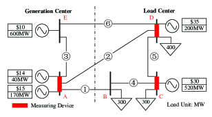
Figure 2: The PJM 5-bus system

1) States of loads and transition probability. Each load is assumed to have 2 states. The loads in Fig. 2 are the base case loads. Another state for each load is half of its base case. The transition probability from one state to another is 0.5.

2) Measuring device transition probability. $p_{T}$ is set 0.5. The attack detection probability is calculated from (8).

3) Costs. The number of target buses at each time step is at most one. The reward weight of each line is 1. The cost $g_{u}$ is set as 0.05.

4) Discount factor. The discount factor $\gamma=0.95$.

We solve the economic dispatch in MATPOWER toolbox in MATLAB. The power flow limit of each line is set 300 MW. We relax the constraint in economic dispatch from $P_{ij}\leq P_{ij}^{\text{M}}$ to $P_{ij}\leq 1.2P_{ij}^{\text{M}}$. We set $V^{\max}=1.1$ p.u. (per unit), $V^{\min}=1.0$ p.u., $n_{V}=5$; $\Delta\theta=5\degree,n_{\theta}=10,\theta_{i}^{\max}$ and $\theta_{i}^{\min}$ are determined from the actual values of bus $i$ in eight load states. For each discretized state, we calculate the lower and upper bounds of each line power flow. One line can be an available target line if the upper bound of its power flow is below the power limit or the lower bound is over the limit.

We solve (14) and (15) to obtain the optimal actions for $2^{3}\times 2^{3}=64$ states and compute the static distribution probabilities of all states. The attack probability of one line is computed as the sum of the distribution probabilities of the states under which the optimal action is to change the congestion pattern of that line. The intrusion probability of one device is the sum of the distribution probabilities of the states under which the optimal action requires manipulating partial or all measurement of that device. The results of the likelihood of data attacks are shown in Figs. 3 and 4.

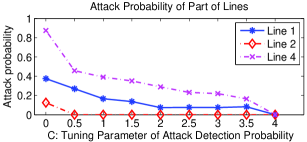
Figure 3: Attack probabilities of part of lines

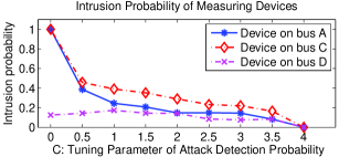
Figure 4: Intrusion probabilities of measuring devices

Generally, as $C$ increases, the attack probability of each line and each measuring device decreases. When $C=0$, it means the launched attack cannot be detected by network operators. In this case, the intruders always choose the action that brings about the maximal immediate net reward. When $C\geq 4$, the net expected reward for each action is negative, hence the optimal action for all states is no attack.

V Conclusion and Discussions

We for the first time analyze the likelihood of cyber data attacks to power systems. We model an intruder’s attack strategy as a Markov Decision Process (MDP). We compute the optimal attack action at a given power system state from an intruder’s perspective. We study the likelihood of cyber data attacks on a small system through simulation. One ongoing work is to apply the method to likelihood analysis of cyber data attacks on larger power systems.

References

- [1] A. Abur and A. G. Exposito, Power system state estimation: theory and implementation. CRC Press, 2004.
- [2] R. B. Bobba, K. M. Rogers, Q. Wang, H. Khurana, K. Nahrstedt, and T. J. Overbye, “Detecting false data injection attacks on DC state estimation,” in Proc. the First Workshop on Secure Control Systems (SCS), 2010.
- [3] J. Chen and A. Abur, “Placement of PMUs to enable bad data detection in state estimation,” IEEE Trans. Power Syst., vol. 21, no. 4, pp. 1608–1615, 2006.
- [4] G. Dán and H. Sandberg, “Stealth attacks and protection schemes for state estimators in power systems,” in Proc. IEEE International Conference on Smart Grid Communications (SmartGridComm), 2010, pp. 214–219.
- [5] D. P. de Farias and B. Van Roy, “The linear programming approach to approximate dynamic programming,” Operations Research, vol. 51, no. 6, pp. 850–865, 2003.
- [6] E. Handschin, F. Schweppe, J. Kohlas, and A. Fiechter, “Bad data analysis for power system state estimation,” IEEE Trans. Power App. Syst., vol. 94, no. 2, pp. 329–337, 1975.
- [7] L. Jia, J. Kim, R. J. Thomas, and L. Tong, “Impact of data quality on real-time locational marginal price,” Power Systems, IEEE Transactions on, vol. 29, no. 2, pp. 627–636, 2014.
- [8] T. Kim and H. Poor, “Strategic protection against data injection attacks on power grids,” IEEE Trans. Smart Grid, vol. 2, no. 2, pp. 326–333, 2011.
- [9] O. Kosut, L. Jia, R. Thomas, and L. Tong, “Malicious data attacks on smart grid state estimation: Attack strategies and countermeasures,” in Proc. IEEE International Conference on Smart Grid Communications (SmartGridComm), 2010, pp. 220–225.
- [10] F. Li and R. Bo, “Small test systems for power system economic studies,” in Power and Energy Society General Meeting, 2010 IEEE. IEEE, 2010, pp. 1–4.
- [11] L. Liu, M. Esmalifalak, Q. Ding, V. A. Emesih, and Z. Han, “Detecting false data injection attacks on power grid by sparse optimization,” IEEE Trans. Smart Grid, vol. 5, no. 2, pp. 612–621, 2014.
- [12] Y. Liu, P. Ning, and M. K. Reiter, “False data injection attacks against state estimation in electric power grids,” ACM Transactions on Information and System Security (TISSEC), vol. 14, no. 1, p. 13, 2011.
- [13] H. M. Merrill and F. C. Schweppe, “Bad data suppression in power system static state estimation,” IEEE Trans. Power App. Syst., no. 6, pp. 2718–2725, 1971.
- [14] A. Monticelli and A. Garcia, “Reliable bad data processing for real-time state estimation,” IEEE Trans. Power App. Syst., no. 5, pp. 1126–1139, 1983.
- [15] M. L. Puterman, “Markov decision processes: Discrete stochastic dynamic programming,” 1994.
- [16] H. Sandberg, A. Teixeira, and K. H. Johansson, “On security indices for state estimators in power networks,” in Proc. the First Workshop on Secure Control Systems (SCS), 2010.
- [17] H. Sedghi and E. Jonckheere, “Statistical structure learning of smart grid for detection of false data injection,” in Proc. IEEE Power and Energy Society General Meeting (PES), 2013, pp. 1–5.
- [18] A. Tajer, S. Kar, H. V. Poor, and S. Cui, “Distributed joint cyber attack detection and state recovery in smart grids,” in Proc. IEEE International Conference on Smart Grid Communications (SmartGridComm), 2011, pp. 202–207.
- [19] M. Wang, P. Gao, S. Ghiocel, J. H. Chow, B. Fardanesh, G. Stefopoulos, and M. P. Razanousky, “Identification of "unobservable" cyber data attacks on power grids,” in Proc. IEEE SmartGridComm, 2014.
- [20] L. Xie, Y. Mo, and B. Sinopoli, “Integrity data attacks in power market operations,” IEEE Trans. Smart Grid, vol. 2, no. 4, pp. 659–666, 2011.
- [21] W. Xu, M. Wang, L. Lai, and A. Tang, “Sparse error correction from nonlinear measurements with applications in bad data detection for power networks,” IEEE Trans. Signal Process., vol. 61, no. 24, pp. 6175–6187, 2013.