The Extreme Walking Behavior in a 331-TC Model

Abstract

It is quite possible that the Technicolor problems are related to the poorly known self-energy expression, or the way chiral symmetry breaking (CSB) is realized in non-abelian gauge theories. Actually, the only known laboratory to test the CSB mechanism is QCD. The TC dynamics may be quite different from the QCD , this fact has led to the walking TC proposal making the new strong interaction almost conformal and changing appreciably its dynamical behavior. There are different ways to obtain of extreme walking (or quasi-conformal) technicolor theories, in this paper we propose an scheme to obtain this behavior based on an extension of the electroweak sector of the standard model, in the context of so called 331-TC model.

I Introduction

The $125$ GeV new resonance discovered at the LHC LHC has many of the characteristics expected for the Standard Model (SM) Higgs boson. If this particle is a composite or an elementary scalar boson is still an open question that probably will be answered in the next LHC run. In recent papers the ATLAS and CMS Collaborationsdiboson reported an experimental anomaly in diboson production with apparent excesses in $WW$, $WZ$ and $ZZ$ channels and this anomaly have inspired a number of theoretical papers proposing as an explanation the production of heavy weak bosons, $W^{\prime}$ and $Z^{\prime}$ .

Thus, it becomes interesting to investigate the possibility of obtaining a light scalar boson in the context of models which features contributions from new heavy weak bosons $W^{\prime}$ and $Z^{\prime}$. In some extensions of the standard model (SM), as in the so called 3-3-1 models3m1 $SU(3)_{{}_{L}}\otimes SU(3)_{{}_{c}}\otimes U(1)_{{}_{X}}$, new massive neutral and charged gauge bosons, $Z^{\prime}$ and $V^{\pm}$, are predicted. The 3-3-1 model is the minimal gauge group that at the leptonic level admits charged fermions and their antiparticles as members of the same multiplet, the predictions of the $GW=SU(2)_{{}_{L}}\otimes U(1)_{{}_{Y}}$ alternative models are leptoquark fermions with electric charges $5/3$ and $4/3$ and bilepton gauge bosons with lepton number $L=\pm 2$. The quantization of electric charge is inevitable in the $G=3m1$ modelsQQ with three non-repetitive fermion generations brea-king generation universality and does not depend on the character of the neutral fermions.

In the Ref.Das was suggested that the gauge symmetry breaking of a specific version of a 3-3-1 model3m1 would be implemented dynamically because at the scale of a few TeVs the $U(1)_{X}$ coupling constant becomes strong and the exotic quark $T$(charge $5/3$) will form a $U(1)_{X}$ condensate breaking $SU(3)_{{}_{L}}\otimes U(1)_{X}$ to the electroweak symmetry. This possibility was explored by us in the Ref.331us assuming a model based on the gauge symmetry $SU(2)_{TC}\otimes SU(3)_{{}_{L}}\otimes SU(3)_{{}_{c}}\otimes U(1)_{{}_{X}}$ , where the electroweak symmetry is broken dynamically by a technifermion condensate, that is characterized by the $SU(2)_{TC}$ Technicolor (TC) gauge group. The early technicolor models weinberg suffered from problems like flavor changing neutral currents (FCNC) and contributions to the electroweak corrections not compatible with the experimental data, as can be seen in the reviews of Ref.tc . However, the TC dynamics may be quite different from the known strong interaction theory, i.e. QCD, this fact has led to the walking TC proposal walk , which are theories where the incompatibility with the experimental data has been sol-ved, making the new strong interaction almost conformal and changing appreciably its dynamical behavior.

We can obtain an almost conformal TC theory, when the fermions are in the fundamental representation, introducing a large number of TC fermions ($n_{TF}$), leading to an almost zero $\beta$ function and flat asymptotic coupling constant. The cost of such procedure may be a large S parameterpeskin incompatible with the high precision electroweak measurements. However, this problem can be solved by assuming that TC fermions are in other representations than the funda-mentalsannino1 and an effective Lagrangian analysis indicates that such models also imply in a light scalar Higgs boson sannino2 . This possibility was also investigated and confirmed through the use of an effective potential for composite operators us1 and through a calculation involving the Bethe-Salpeter equation (BSE) for the scalar state us2 .

The reason for the existence of the different models (or different potentials) for a composite scalar boson, is a consequence of our poor knowledge of the strongly interacting theories, that is reflected in the many choices of parameters in the effective potentials. The possibility of obtaining a light composite scalar according to the approach discussed in Ref.us1 , is that this result is a direct consequence of extreme walking (or quasi-conformal) technicolor theories, where the asymptotic self-energy behavior is described by Irregular form of TC fermionsus1 ; us2

$$\Sigma^{(0)}(p^{2})\sim\mu\left[1+bg^{2}(\mu^{2})\ln\left(p^{2}/\mu^{2}\right)\right]^{-\gamma}\,.$$ (1)

In the Ref.twoscale we considered the possibility of a light composite scalar boson arising from mass mixing between a relatively light and heavy scalar singlets from a see-saw mechanism expected to occur in two-scale Technicolor (TC) models and we identified that, regardless of the approach used for generating a light composite scalar boson, the behavior exhibited by extreme walking technicolor theories, is the main feature needed to produce a light composite scalar boson compatible with the boson observed at the LHC.

After this brief motivation of the importance of extreme walking behavior to generate a light composite scalar boson in TC models, in addition to possibility of 331-TC model contain the necessary requirements to explain the anomaly in diboson production, in this paper we propose an scheme to obtain the quasi-conformal behavior based on an extension of the electroweak sector of the standard model, 331-TC model ($SU(N)_{TC}\otimes[SU(3)_{{}_{L}}\otimes SU(3)_{{}_{c}}\otimes U(1)_{{}_{X}}]$). In this model only exotic techniquarks ($U^{\prime},D^{\prime}$) will acquire dynamically generated mass due $U(1)_{X}$ interaction at $\Lambda_{{}_{331}}\!\!\sim\!O(TeV)$ . The terminology exotic refers to nomenclature used in $331$ models to designate the allocation of fractional charges assigned to the new quarks ($T,D$). In analogy with this nomenclature ($U^{\prime},D^{\prime}$) are termed ”exotic techniquarks”, and all techniquarks are in the fundamental representationn, $(R=F)$, of $SU(N)_{TC}$.

Technicolor models with fermions in the fundamental representation are subject to strong experimental constraints that comes from the limits on the $S$ parameter. In our case, the contribution due to the TC sector should still lead to a value to the S parameter compatible with the experimental data. At low energies, i.e. at the scale associated with electroweak symmetry breaking, we should only consider the contribution of four techniquarks because (U ’and D’) are singlets of $SU(2)_{L}$ and do not contribute directly to the bosons (W and Z) masses

The exotic technifermions will present the extreme walking behavior, the usual techniquarks ($U,D$) will present the known asymptotic self-energy behavior predicted by the operator product expansion(OPE)ope . The exotic techniquarks will have two different energy scales and the 331-TC model corresponds to an example of two-scale Technicolor (TC) model. This article is organized as follows: In section II we present the $U(1)_{X}$ contribution to fermions and technifermions self-energy, in section III we compute the dynamically generated masses to heavy exotic quarks $(T,S,D)$ and techniquarks $(U^{\prime},D^{\prime})$ , where we reproduce the results obtained in Ref.Das for heavy exotic quarks. In the section IV we illustrate how to obtain the extreme walking behavior in the context of 331-TC model and Section V contains our conclusions.

II The $U(1)_{X}$ Contribution to Fermions and Technifermions Self-Energy

As described in Refs.Das ; 331us the gauge symmetry breaking in 3-3-1 models can be implemented dynamically because at the scale of a few TeVs the $U(1)_{X}$ coupling constant becomes strong. The exotic quark $T$ introduced will form a condensate breaking $SU(3)_{{}_{L}}\otimes U(1)_{X}$ to electroweak symmetry, in this paper we will numerically determine the $U(1)_{X}$ contribution to dynamic mass of exotic quarks $(T,S,D)$ and techniquarks $(U^{\prime},D^{\prime})$ that appear in the fermionic content of the model331us following the same procedure described in Ref.Das . The Schwinger-Dyson equation for quarks(techni-quarks) due to $U(1)_{X}$ interaction can be written asDas ; 331us

$$S^{-1}(p)=\not{\!\!p}-i\int\frac{d^{4}q}{(2\pi)^{4}}\Gamma_{\mu}(p,q)S(q)\Gamma_{\nu}D^{\mu\nu}_{{}_{M_{Z^{\prime}}}}(p-q)$$ (2)

where in the equation above we assumed the rainbow approximation for the vertex $\Gamma_{\mu,\nu}$, with $\Gamma_{\mu,\nu}=(g_{{}_{V}}\gamma_{\mu,\nu}-g_{{}_{A}}\gamma_{\mu,\nu}\gamma_{5})$, $g_{{}_{V}}=g^{2}_{X}(Y_{{}_{L}}+Y_{{}_{R}})/4$ and $g_{{}_{A}}=g^{2}_{X}(Y_{{}_{L}}-Y_{{}_{R}})/4$, where $Y_{i}$ are $U(1)_{{}_{X}}$ hypercharges attributed at chiral components of the exotic quarks(techniquarks).

With the purpose of simplifying the calculations it is convenient to choose the Landau Gauge. In this case the $Z^{\prime}$ propagator can be written in the following form

$$iD^{\mu\nu}_{{}_{M_{Z^{\prime}}}}(p-q)=-i\frac{\left[g_{\mu\nu}-(p-q)_{\mu}(p-q)_{\nu}/(p-q)^{2}\right]}{(p-q)^{2}-M^{2}_{Z^{\prime}}}.$$

Writing the quark propagator as $i{S}_{{}_{F}}^{\,-1}(p)=i(\not{p}-\Sigma_{X}(p^{2}))$, and considering the equation above, we finally can write in the euclidean space the gap equation for $\Sigma(p^{2})$Das

$$\Sigma_{X}(p^{2})= a\int_{0}^{p^{2}}d^{2}qq^{2}\frac{\Sigma_{X}(q^{2})}{[q^{2}+\Sigma^{2}_{X}(q^{2})]}\frac{1}{[p^{2}+M^{2}_{Z^{\prime}}]}+$$ (3)

$$a\int_{p^{2}}^{\Lambda^{2}}d^{2}qq^{2}\frac{\Sigma_{X}(q^{2})}{[q^{2}+\Sigma^{2}_{X}(q^{2})]}\frac{1}{[q^{2}+M^{2}_{Z^{\prime}}]}$$

where $a=\frac{g^{2}_{{}_{X}}Y_{{}_{L}}Y_{{}_{R}}}{16\pi^{2}}=\beta Y_{{}_{L}}Y_{{}_{R}}$. To obtain the last equation we assumed the angle approximation to transform the term
$\frac{1}{(p-q)^{2}+M^{2}_{Z^{\prime}}}$ as

$$\frac{1}{(p-q)^{2}+M^{2}_{Z^{\prime}}}=\frac{\theta(p-q)}{p^{2}+M^{2}_{Z^{\prime}}}+\frac{\theta(q-p)}{q^{2}+M^{2}_{Z^{\prime}}}.$$ (4)

The integral equation described above can be transformed into a differential equation for $f(x)$ introducing the new variables $x=\frac{p^{2}}{M^{2}}$, with $f(x)=\frac{\Sigma_{X}(x)}{M}$ and $\alpha=\frac{M_{Z^{\prime}}}{M}$ that we reproduce below

$$f^{\prime\prime}(x)+\frac{2}{x+\alpha^{2}}f^{\prime}(x)+\frac{\beta Y_{{}_{L}}Y_{{}_{R}}}{(x+\alpha^{2})^{2}}\frac{xf(x)}{(x+f^{2}(x))}=0,$$ (5)

where $M\equiv\Sigma_{X}(0)$ is the dynamical mass of exotic quarks(or techniquarks) generated by $U(1)_{X}$ interaction and the respective boundary conditions for $f(x)$ are $f(0)=1$ and $f^{\prime}(0)\\ =0$. In order to obtain the mass spectrum generated due to $U(1)_{X}$ interaction, we follow the same procedure described in Ref.Das where the $(Y_{i})$ hipercharges of exotic quarks $(T,S,\\ D)$ were assumed according to the table 1 and we include the corresponding hipercharges of exotic techniquarks $(U^{\prime},D^{\prime})$ 331us that are singlets of $SU(3)_{c}$.

Table 1: $(Y_{i})$ Hipercharges of exotic quarks $(T,S,D)$ and exotic techniquarks $(U^{\prime},D^{\prime})$.

$Y_{L}$	$Y_{R}$	Exotic Fermion	Charge
		(Technifermion)
$-4/3$	$-10/3$	T	$+5/3$
$+2/3$	$+8/3$	D,S	$-4/3$
$-1$	$-3$	U’	$+3/2$
$+1$	$+3$	D’	$-3/2$

III Dynamically generated masses of exotic quarks and techniquarks due $U(1)_{X}$ contribution

As commented in the previous section we follow the same procedure described in Ref.Das , therefore, in order to get an estimate of the $U(1)_{X}$ dynamically generated mass, for exotic fermions(or technifermions), we will numerically solve the Eq.(3) imposing an ultraviolet cutoff $\Lambda$ on this equation. If the gap equation accepts a $M_{T}$ solution($M_{T}$ is mass of exotic quark (T)), then the gauge symmetry $SU(3)_{{}_{L}}\otimes U(1)_{{}_{X}}$ is dynamically broken to $SU(2)_{{}_{L}}\otimes U(1)_{{}_{Y}}$ and the $Z^{\prime}$, $V^{\pm}$, and $U^{\pm\pm}$ gauge bosons become massive. The $Z^{\prime}$ mass is given by $M_{Z^{\prime}}=\frac{g_{X}}{4}F_{\Pi}\left(Y^{T}_{L}-Y^{T}_{R}\right)$ , where $F_{\Pi}$ is the pseudoscalar decay constant and we calculate it using the Pagels-Stokar approximation that is given by

$$F_{\Pi}=\frac{1}{4\pi^{2}}\int\!\!\frac{dp^{2}p^{2}}{(p^{2}+\Sigma^{2}_{X}(p^{2}))^{2}}\!\!\left[\Sigma^{2}_{X}(p^{2})-\frac{p^{2}}{2}\frac{d\Sigma_{X}(p^{2})}{dp^{2}}\Sigma_{X}(p^{2})\right]$$ (6)

Assuming the set of variables described below of Eq.(4), the above equation together with the definition of $M_{Z^{\prime}}$, allows to write the Pagels-Stokar relation as

$$1=\frac{\beta}{\alpha^{2}}\int^{\left(\!\frac{\Lambda}{M_{Z^{\prime}}}\!\right)^{2}\!\!\alpha^{2}}_{0}\!\!\!\!\!\!\!\!\frac{dxx}{(x+f^{2}(x))^{2}}\!\!\left[f^{2}(x)-\frac{x}{2}\frac{df(x)}{dx}f(x)\right],$$ (7)

where the coefficients $\alpha$ and $\beta$ were defined in the previous section.

According to the description given in Das the consistency requirement imposed about the solution of Eq.(5) is that the mass of the exchanged particle $Z^{\prime}$(or $\alpha=\frac{M_{Z^{\prime}}}{M}$) has to be equal to $Z^{\prime}$ mass (or $\alpha$) obtained using Eq.(7). In other words the solutions of the gap equation Eq.(5) are iteratively improved by starting with a trial guess for the exchanged boson mass and then comparing it with the predicted mass obtained using the Eq.(7). In the Fig I we show the behavior of Eq.(7) assuming the numerical solution of Eq. (5) for $\Lambda=42TeV$, $M_{Z^{\prime}}=2TeV$ as a function of parameters $\alpha$ and $\beta$. In the table II we show the results obtained for the dynamically generated masses for heavy exotic quarks $(T,S,D)$ and exotic techniquarks $(U^{\prime},D^{\prime})$ , where we reproduce the results obtained in Ref.Das for heavy exotic quarks .

Table 2: The dynamically generated heavy exotic quarks(techniquarks) masses for different $U(1)_{X}$ gauge coupling $g_{X}$ and cutoff $\Lambda$.

$\Lambda(TeV)$	$M_{Z^{\prime}}(TeV)$	$g_{X}$	$\beta$	$M_{T}(TeV)$	$M_{S,D}(TeV)$	$M_{U^{\prime},D^{\prime}}(TeV)$
42	2.00	2.576	0.0420	5.73	0.76	0.82
42	2.50	2.576	0.0420	7.57	0.55	0.67
90	3.00	2.541	0.0409	8.22	0.92	1.12
162	4.00	2.526	0.0404	10.64	1.22	1.41
196	4.50	2.523	0.0403	11.94	1.34	1.47
247	5.00	2.514	0.0400	13.16	1.52	1.75

Figure 1: Plot of numerical solution of Eqs. (5) and (7) as function of parameters $\alpha$ and $\beta$ to $\Lambda=42TeV$, $M_{Z^{\prime}}=2TeV$. To $g_{X}=2.576$($\beta=0.042$) we get $M_{T}=5.73TeV$($\alpha=0.349$) which corresponds to the first value obtained for $M_{T}$ described in Ref.Das .

IV The Extreme Walking Behavior in a 331-TC Model

Theories with large anomalous dimensions ($\gamma_{m}>1$) are quite desirable for technicolor phenomenology takeuchi ; tc , it is known for a long date that four-fermion interactions are responsible for harder self-energy solutions in non-Abelian gauge theories ($\gamma_{m}\sim 2$)takeuchi ; miranski . In the model considered in this work we show that due to the $U(1)_{X}$ interaction only the exotic techniquarks ($U^{\prime},D^{\prime}$) will acquire an dynamical mass $M_{U^{\prime}}=M_{D^{\prime}}=O(TeV)$ at $\Lambda_{331}\sim O(TeV)$. The result is that at this energy scale a bare mass appears in the (TC) Schwinger-Dyson equation assigned to exotic techniquarks, ($U^{\prime},D^{\prime}$) , what leads to a very ”hard” self-energy, or a self-energy of the irregular type, Eq.(1), only for exotic techniquarks ($U^{\prime},D^{\prime}$). In this section considering a four-fermion approximation for $U(1)_{X}$ interaction associated to these techniquarks we will show that the results for $M_{U^{\prime}}=M_{D^{\prime}}=O(TeV)$ are of the same order as obtained in the previous section, in this case $F_{\Pi}$ equation is given by

$$F^{2}_{\Pi}=\frac{1}{4\pi^{2}}\int\!\!\frac{dp^{2}p^{2}M^{2}_{X}}{(p^{2}+M^{2}_{X})^{2}}$$ (8)

where $M_{X}=M_{U^{\prime}}=M_{D^{\prime}}$ or $M_{T}$. As in the previous section, the equation above together with the definition of $M_{Z^{\prime}}$, allows us to write

$$1\approx\frac{\beta}{\alpha^{2}}\int\!\!\frac{dp^{2}p^{2}}{(p^{2}+M^{2}_{X})^{2}}.$$ (9)

For a similar choice of parameters, used in the previous section, for example $\Lambda=42$ TeV, $\beta=0.042$ and $M_{Z^{\prime}}=2.5$ TeV we obtain $M_{T}\approx 6.3$TeV and $M_{U^{\prime}}=M_{D^{\prime}}\approx 0.6$TeV so that the contribution due $U(1)_{X}$ to the mass of exotic techniquarks can be approximated by a four-fermion interaction and the exotic techniquarks exhibit a self-energy behavior of the irregular type.

To illustrated the extreme walking behavior exhibited only by the exotic technifermions we consider the full gap equation for the ”exotic techniquark U’” that contains the sum of two contributions, the $U(1)_{X}$ interaction and TC interaction, and we consider the presence of dynamically massive technigluons. The problems for chiral symmetry breaking in this case have been discussed recently, where confinement may play an important roleagn ; rdn ; fdn . In this work we consider that technigluons acquire a dynamical mass along the line of QCD as proposed by CornwallCornwall many years ago and the dynamical technigluon mass behaves asagn ; rdn

$$m^{2}_{tg}(k^{2})=\frac{m^{4}_{tg}(0)}{k^{2}+m^{2}_{tg}(0)},$$ (10)

with $m_{tg}(0)\approx\Lambda_{TC}$ and the technifermion dynamical mass will be given by

$$\!\!\!\!\!M_{TC}(p^{2})=\frac{C_{2}}{(2\pi)^{4}}\int\!\!\frac{K(g,p)d^{4}k}{[k^{2}+M^{2}_{TC}(k^{2})]},$$ (11)

where

$$K(g,p)=\frac{3\bar{g}^{2}_{tc}(p-k)M_{TC}(k^{2})}{(p-k)^{2}+m_{tg}^{2}((p-k)^{2})}$$

$M_{TC}(p^{2})$ is the dynamical techniquark mass, and $C_{2}$ is the Casimir operator for the technifermionic representation with effective TC coupling ${\bar{g}}_{tc}$, given by

$${\bar{g}}^{2}_{tg}(p^{2})=\frac{1}{b_{TC}\ln[(p^{2}+4m^{2}_{tg}(p^{2}))/\Lambda_{TC}^{2}]}\,,$$ (12)

in this expression $b_{TC}$ is the first $\beta_{TC}$ function coefficient and we consider the Landau gauge. Similarly to the previous section the integral equation described by Eq.(11) can be transformed into a differential equation for $h(x)$ introducing the new variables $x=\frac{p^{2}}{M^{2}_{TC}(0)}$, with $h(x)=\frac{M_{TC}(x)}{M_{TC}(0)}$ and $\delta=\frac{m_{tg}(0)}{M_{TC}(0)}$ we obtain

$$h^{\prime\prime}(x)+\frac{2}{x+\delta^{2}}h^{\prime}(x)+\frac{3C_{2}g^{2}_{TC}(x)}{16\pi^{2}(x+\delta^{2})^{2}}\frac{xh(x)}{(x+h^{2}(x))}=0.$$ (13)

The full gap equation for the ”exotic techniquark U’” can be written as

$$M_{U^{\prime}}(x)=M_{TC}(0)h(x)+M_{X}(4f),$$ (14)

in the Fig.(2a)[Blue curve] we show the behavior of $M_{TC}(x)=\frac{\langle\bar{U}{U}\rangle}{\Lambda^{2}}$, that corresponds to the dynamical mass generated for the the usual techniquarks $(U,D)$ obtained with Eq.(13). In the Fig.(2b)[Red curve] we include the contribution of $U(1)_{X}$ effective four-fermion interaction and we show the behavior of the dynamical mass generated for the exotic techniquarks $(U^{\prime},D^{\prime})$, which is described by $M_{U^{\prime}}(x)=\frac{\langle\bar{U^{\prime}}{U^{\prime}}\rangle}{\Lambda^{2}}$.

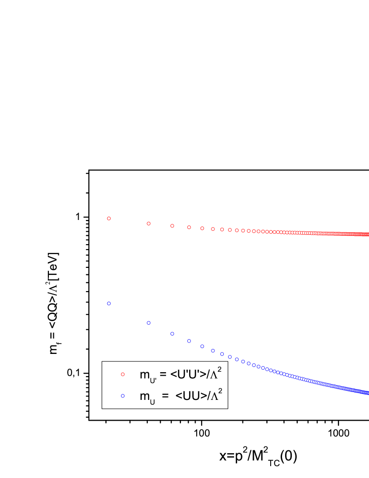
Figure 2: In this figure we plot the behavior of $M_{TC}(x)=\frac{\langle\bar{U}{U}\rangle}{\Lambda^{2}}$ obtained with Eq.(13) to $N_{TC}=SU(2)_{TC}$ and $n_{TF}=6$ fig.(2a)[curve in Blue] and in the fig.(2b)[curve in Red] we show the behavior of dynamical mass generated for the exotic techniquarks $(U^{\prime},D^{\prime})$, given by $M_{U^{\prime}}(x)=\frac{\langle\bar{U^{\prime}}{U^{\prime}}\rangle}{\Lambda^{2}}$.

V Conclusions

In the Refs.us1 ; us2 ; us3 ; twoscale we discussed the possibility of obtaining a light composite TC scalar boson, this result is a direct consequence of extreme walking (or quasi-conformal) technicolor theories, where the asymptotic self-energy behavior is described by Eq.(1). The extreme walking technicolor can be obtained in three different ways and in this paper we propose an scheme to obtain the quasi-conformal behavior based on an extension of the electroweak sector of the standard model, in the so called 331-TC model ($SU(N)_{TC}\otimes SU(3)_{{}_{L}}\otimes SU(3)_{{}_{c}}\otimes U(1)_{{}_{X}}$), where the exotic quark $T$ introduced will form a $U(1)_{X}$ condensate $(\langle\bar{T}T\rangle)$ breaking $SU(3)_{{}_{L}}\otimes U(1)_{X}$ to electroweak symmetry that is broken by an usual technifermion condensate. As the comment presented in the introductory section, 3-3-1 models predicted new massive weak gauge bosons, $Z^{\prime}$ and $V^{\pm}$, and this model has the necessary requirements to explain the reported diboson anomaly.

Following the same procedure described in Ref.Das , the solutions of the gap equation, Eq.(5), were iteratively improved by starting with a trial guess for the exchanged boson mass and then comparing it with the predicted mass obtained using the Eq.(7). In the table II we show the results obtained for the dynamically generated masses of heavy exotic quarks $(T,S,D)$ and exotic techniquarks $(U^{\prime},D^{\prime})$ , where we reproduce the results obtained in Ref.Das for heavy exotic quarks. In Ref.an3 we discuss a mechanism for the dynamical mass generation, including the mass generation for the t quark, in the case of grand unified theories that incorporate quarks and techniquarks. We expect that a similar mechanism to the one described in an3 can be developed and incorporated in the present model. In the section 4 we show that the results obtained in the table II, ($M_{U^{\prime}}=M_{D^{\prime}}=O(TeV)$), are of the same order as the ones obtained with a four-fermion approximation for the $U(1)_{X}$ interaction and in the Fig.2 [Red Curve ] we show the extreme walking behavior displayed only by exotic techniquarks ($U^{\prime},D^{\prime}$) due to their strong $U(1)_{X}$ interaction because $Y^{U^{\prime}}_{L}Y^{U^{\prime}}_{R}=3$ (see table I). The exotic technifermions have two different energy scales and the 331-TC model corresponds to an example of two-scale Technicolor (TC) model, in the Ref.twoscale we considered the possibility of a light TC composite boson arising from mass mixing between a relatively light and heavy composite scalar singlets from a see-saw mechanism expected to occur in two-scale TC model. We emphasize that the see-saw mechanism expected to occur in this model is not exactly the same one described in the Ref[16], in the model proposed the extreme walking behavior displayed by exotic techniquarks is due to their strong $U(1)_{X}$ interaction and in this case in Eq.(1), $\mu\approx\Lambda_{2}=\Lambda_{331}$, and $\Lambda_{2}$ it is not generated by the TC sector. In order to provide a example we consider the $SU(2)_{TC}$ case with the technifermionic content showed in[6], where $n_{TF}=6$. With this we obtain $m_{\phi_{1}}\sim 124$ GeV, $m_{\phi_{2}}\sim 8.3$TeV to $\Lambda_{331}=3TeV$ and $\Lambda_{ETC}\approx 90$TeV. Therefore, in this scenario it is possible to obtain a light composite TC scalar boson and include the necessary requirements to explain the diboson anomaly, the determination of the scalar spectrum for composite Higgs bosons of this model will be presented in detail in a future work.

- (1) ATLAS Collaboration, Phys. Lett. B 716, 1 (2012); CMS Collaboration, Phys. Lett. B 716, 30 (2012).
- (2) G. Aad et al. [ATLAS Collaboration], arXiv:1506.00962 [hep-ex]; V. Khachatryan et. al. [CMS Collaboration], JHEP 08 173 (2014), V. Khachatryan et. al. [CMS Collaboration], JHEP 08 174 (2014).
- (3) M. Singer, J. W. F. Valle and J. Schechter, Phys. Rev. D 22, 738 (1980); F. Pisano and V. Pleitez, Phys. Rev. D 46, 410 (1992); P. H. Frampton, Phys. Rev. Lett. 69, 2889 (1992); R. Foot, H. N. Long and Tuan A. Tran, Phys. Rev. D 50, 34 (1994); H. N. Long, Phys. Rev. D 54, 4691 (1996); F. Pisano and V. Pleitez, Phys. Rev. D 51, 3865 (1995); Adrian Palcu, Mod. Phys. Lett. A 24, 2175 (2009).
- (4) F. Pisano, Mod. Phys. Lett A 11, 2639 (1996); A. Doff and F. Pisano, Mod. Phys. Lett A 14, 1133 (1999); A. Doff and F. Pisano, Phys.Rev. D 63, 097903 (2001); C. A. de S. Pires and O. P. Ravinez, Phys. Rev. D 58, 035008 (1998); C. A. de S. Pires, Phys. Rev. D 60, 075013 (1999); P. V. Dong and H. N. Long, Int. J. Mod. Phys. A 21, 6677 (2006).
- (5) Prasanta Das and Pankaj Jain, Phys. Rev. D 62, 075001 (2000).
- (6) A. Doff, Phys. Rev. D 81, 117702 (2010).
- (7) H. D. Politzer, Nucl. Phys. B 117, 397 (1976).
- (8) L. Susskind, Phys. Rev. D 20 , 2619 (1979); S. Dimopoulos and L. Susskind, Nucl. Phys. B 155 , 237 (1979); S. Weinberg, Phys. Rev. D 13, 974 (1976); S. Weinberg, Phys. Rev. D 19 1277 (1979).
- (9) C. T. Hill and E. H. Simmons, Phys. Rept. 381, 235 (2003) [Erratum-ibid. 390, 553 (2004)]; F. Sannino, hep-ph/0911.0931; K. Lane, Technicolor 2000 , Lectures at the LNF Spring School in Nuclear, Subnuclear and Astroparticle Physics, Frascati (Rome), Italy, May 15-20, 2000.
- (10) B. Holdom, Phys. Rev. D 24,1441 (1981); Phys. Lett. B 150, 301 (1985); T. Appelquist, D. Karabali e L. C. R. Wijewardhana, Phys. Rev. Lett. 57, 957 (1986); T. Appelquist and L. C. R. Wijewardhana, Phys. Rev. D 36, 568 (1987); T. Appelquist, M. Piai and R. Shrock, Phys. Lett. B 593 , 175 (2004). M. E. Peskin and T. Takeuchi, Phys. Rev. Lett. 65, 964 (1990); Phys. Rev. D 46, 381 (1992).
- (11) M. E. Peskin and T. Takeuchi, Phys. Rev. Lett. 65, 964 (1990); Phys. Rev. D 46, 381 (1992).
- (12) F. Sannino and K. Tuominen, Phys. Rev. D 71, 051901 (2005); R. Foadi, M. T. Frandsen, T. A. Ryttov and F. Sannino, Phys. Rev. D 76, 055005 (2007).
- (13) T. A. Ryttov and F. Sannino, Phys. Rev. D 78, 115010 (2008).
- (14) A. Doff, A. A. Natale and P. S. Rodrigues da Silva, Phys. Rev. D 77, 075012 (2008).
- (15) A. Doff, A. A. Natale and P. S. Rodrigues da Silva, Phys. Rev. D 80, 055005 (2009).
- (16) A. Doff and A. A. Natale, Phys. Lett. B 748, 55 (2015).
- (17) A. Doff, Eur.Phys.J. C 60 285-289,(2009).
- (18) T. Takeuchi, Phys. Rev. D 40, 2697 (1989); K.-I. Kondo, S. Shuto and K. Yamawaki, Mod. Phys. Lett. A 6, 3385 (1991).
- (19) V. A. Miransky and K. Yamawaki, Mod. Phys. Lett. A 04, 129 (1989); V. A Miransky, M. Tanabashi and K. Yamawaki, Phys. Lett. B 221, 177 (1989).
- (20) H. Pagels and S. Stokar, Phys. Rev. D20, 2947 (1979).
- (21) A. Doff, F. A. Machado and A. A. Natale, New. J. Phys. 14, 103043 (2012).
- (22) J. M. Cornwall, Phys. Rev. D 26, 1453 (1982).
- (23) A. C. Aguilar and A. A. Natale, JHEP 0408, 057 (2004).
- (24) R. M. Capdevilla, A. Doff and A. A. Natale, Phys. Lett. B 744, 325 (2015).
- (25) A. Doff, E. G. S. Luna and A. A. Natale, Phys. Rev. D 88, 055008 (2013).
- (26) A. Doff and A. A. Natale, Eur.Phys.J. C 32, 417 (2003). Phys. Rev. D 88, 055008 (2013).