Optimal Qubit Control Using Single-Flux Quantum Pulses

Abstract

Single flux quantum pulses are a natural candidate for on-chip control of superconducting qubits. We show that they can drive high-fidelity single-qubit rotations—even in leaky transmon qubits—if the pulse sequence is suitably optimized. We achieve this objective by showing that, for these restricted all-digital pulses, genetic algorithms can be made to converge to arbitrarily low error, verified up to a reduction in gate error by 2 orders of magnitude compared to an evenly spaced pulse train. Timing jitter of the pulses is taken into account, exploring the robustness of our optimized sequence. This approach takes us one step further towards on-chip qubit controls.

I Introduction

Rapid single flux quantum (RSFQ) technology has been and is originally pursued as an ultra-high-speed classical computing platform Likharev and Semenov (1991); Likharev (2012). The ability to generate reproducible identical pulses at a high clock rate has been demonstrated in integrated circuits Castellano et al. (2007). Next to its original motivation of ultrafast digital circuits, this ability makes RSFQ technology a highly viable candidate for the on-chip generation of control pulses and readout for quantum computers based on Josephson devices Orlando et al. (2002); Feldman and Bocko (2001); Ohki et al. (2007); Semenov and Averin (2003); Fedorov et al. (2007, 2014). The switching time lies in the picosecond range, leading to fast quantum gates Ohki et al. (2005), but the timing of the single-voltage pulses to control the devices is a major challenge Gaj et al. (1997). The integration capabilities of RSFQ technology are compatible with scaling quantum processors McDermott and Vavilov (2014); Fowler et al. (2012); for example, one can load pulse sequences into shift registers Mukhanov (1993). Then again, the present-day control scheme is based on room-temperature electronics, whose signals are transmitted as analog signals through filters into a cryostat, which creates large physical overhead.

Besides these engineering considerations, both techniques present distinct paradigms for control design. Room-temperature generators have high-amplitude resolution (currently, 12 bits are typical) at limited speed; thus, methods of analog pulse shaping can be applied Glaser et al. (2015) to approximating the experiment with high accuracy. This approximation has been done in superconducting qubits, e.g., within the derivative removal by adiabatic gate (DRAG) and wah-wah method Motzoi et al. (2009); Schutjens et al. (2013), that suppress leakage into higher energy levels. These pulses can be readily calibrated using a protocol named Ad-HOC Egger and Wilhelm (2014).

On the other hand, SFQ pulses only have a single bit of amplitude resolution: in a given time interval, there is either a pulse or not. The RSFQ sequence proposed in Ref. McDermott and Vavilov (2014) again reveals the challenge of balancing gate speed with suppression of leakage in transmon qubits similar to DRAG, demonstrating the need for advanced pulse design methods which cannot be solved by evenly spaced pulses alone. While their amplitude resolution is minimal, an RSFQ sequence has a very short time constant of the pulse train—much shorter than the intrinsic frequencies of the qubit system—that can be expected to simulate analog control. To explore this matter, one needs to depart from the conventional optimal-control paradigms as reviewed in Ref. Glaser et al. (2015), which often involve gradients, and focus instead on digital control and algorithms that can optimize these fully discrete controls.

In this paper we show that optimal-control methods, based on genetic algorithms adapted to digital control, can be used to improve gate operations with trains of SFQ pulses. The single bit of amplitude resolution is encoded in a discretized time evolution, which also limits possible clock frequencies. We show that uneven and relatively densely populated bit-string pulse sequences can be used to suppress leakage as well as to drastically reduce gate times up to the speed limit. We also verify that optimized pulse sequences are robust against timing jitter, the degree of which depends on the clock integration.

II SFQ control

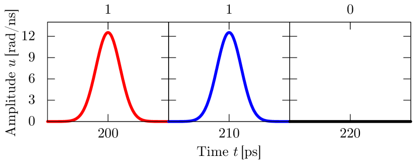
Figure 1: (Color online) Time slicing of the evolution: in each frame, the control amplitude $u(t)$ either has a Gaussian shape (1) or vanishes (0). Therefore, only two unitary operators $\boldsymbol{U}_{i}$ need to be calculated, each with a duration of $2t_{c}$ (here, 10 ps). The gap between two consecutive pulses is always an integer multiple of $2t_{c}$.

Figure 2: Bit-string representation of the pulse sequence before (top) and after (bottom) the optimization for a gate time of 20 ns. A vertical black line indicates the time when a pulse is applied, and white space the duration of the free evolution.

As a simple model, we use a qubit with a leakage level such as the transmon qubit Koch et al. (2007); Girvin (2011) that can be controlled with voltage pulses. Our single-qubit target gate is a rotation around the $y$ axis, i.e., a Pauli-$Y$ gate with an arbitrary global phase. The time-dependent system Hamiltonian in units of $\hbar$ reads

$$\boldsymbol{H}(t)=\boldsymbol{H}_{0}+u(t)\boldsymbol{H}_{1}\,,$$ (1)

with drift and control terms

$$\boldsymbol{H}_{0}=\begin{bmatrix}0&0&0\\ 0&\omega&0\\ 0&0&2\omega+\Delta\end{bmatrix}\,,\quad\boldsymbol{H}_{1}=\begin{bmatrix}0&\frac{-i}{2}&0\\ \frac{i}{2}&0&\frac{-i}{\sqrt{2}}\\ 0&\frac{i}{\sqrt{2}}&0\end{bmatrix}\,,$$ (2)

where $\omega$ is the qubit’s angular frequency and $\Delta$ the anharmonicity of the third level. Gate operations are performed by changing the control amplitude $u(t)$. However, instead of finding a proper pulse shape with a duration of several nanoseconds, we apply a single-picosecond pulse repeatedly. This pulse is switched on and off as stored in a shift register and controlled by a clock. The pulse shape we use is a truncated Gaussian with standard deviation $\tau$ and total duration $2t_{c}$

$$u(t)=\frac{\delta\theta}{\sqrt{2\pi}\tau}e^{-t^{2}/2\tau^{2}}\qquad\int_{-t_{c}}^{t_{c}}u(t)dt\approx\delta\theta\,.$$ (3)

The area $\delta\theta$ is approximated by the numerical integration of the pulse shape. It matches the rotation angle on the Bloch sphere for an infinitely narrow $\delta$ pulse. To flip the Bloch vector around the $y$ axis, we can thus set a lower bound of $n=\pi/\delta\theta$ pulses. Note that the three-level model outlined in Eq. (2) is sufficient to describe the qubit dynamics — we perform a posteriori verifications with more levels and find no discernible difference.

We simulate our system by slicing the total gate time into $N$ time steps of length $2t_{c}$, i.e., the clock period. Choosing $\tau$ accordingly ensures that the applied voltage pulse shape $u(t)$ vanishes at the beginning and the end of a the time interval. We interpret the free evolution of the system in a time interval $[t_{i},t_{i}+2t_{c}]$ as a pulse with zero amplitude. Figure 1 shows an example of two consecutive pulses followed by an interval without an applied pulse. The time difference between two applied pulses is always a positive integer multiple of the pixel length $2t_{c}$. For each interval $[t_{i},t_{i}+2t_{c}]$, the time evolution is captured in a unitary matrix $\boldsymbol{U}(t_{i})\equiv\boldsymbol{U}(t_{i}+2t_{c},t_{i})$. Since we apply a single pulse only if it is necessary, each unitary is chosen out of a given database containing just two unitary operators, $\boldsymbol{U}_{0}$ and $\boldsymbol{U}_{1}$. For both our work and future practical applications, this can be done efficiently by storing all of the relevant system parameters in this database. Therefore, the pulse sequence can be represented as bit string, where zeros represent a free-evolution interval $\boldsymbol{U}_{0}$ and ones an applied voltage pulse $\boldsymbol{U}_{1}$; see Fig. 2. The total time evolution reads

$$\boldsymbol{U}(t_{\textrm{gate}})=\prod_{i=N-1}^{0}\boldsymbol{U}(t_{i})=\boldsymbol{U}(t_{N-1})\cdots\boldsymbol{U}(t_{0})\,.$$ (4)

The database that the unitaries are chosen from consists of

$$\boldsymbol{U}_{0} =\exp\left(-2it_{c}\boldsymbol{H}_{0}\right)=\boldsymbol{U}_{0}(2t_{c})$$ (5)

$$\boldsymbol{U}_{1} =\boldsymbol{U}_{0}(t_{c})\left[\mathcal{T}\exp\left(-i\int_{-t_{c}}^{t_{c}}\boldsymbol{H}(t)dt\right)\right]\boldsymbol{U}_{0}(-t_{c})\,.$$ (6)

Any adjustment in the experiment can be captured in the database and all characterization of the pulses has to be done once in order to find these two database entries.

The target gate is a Pauli-$Y$ gate, where we allow an arbitrary phase for the leakage level, and the global phase is neglected when using an appropriate fidelity function [Eq. (8)],

$$\boldsymbol{U}_{\mathrm{target}}=\begin{bmatrix}0&-1&0\\ 1&0&0\\ 0&0&e^{i\varphi}\end{bmatrix}\,.$$ (7)

We optimize our time evolution within the computational subspace of the qubit. The average fidelity function therefore reads Rebentrost and Wilhelm (2009)

$$\Phi=\frac{1}{4}\left|\text{tr}\left\{\boldsymbol{U}^{\dagger}_{\mathrm{target}}\boldsymbol{P}_{Q}\boldsymbol{U}(t_{\mathrm{gate}})\boldsymbol{P}_{Q}\right\}\right|^{2}\,,$$ (8)

with the projector onto the qubit subspace $\boldsymbol{P}_{Q}$.

Typical values for a transmon qubit Koch et al. (2007) are for the qubit transition frequency $\omega/2\pi=5$ GHz and its anharmonicity $\Delta/2\pi=-200$ MHz. The pulse area and duration are set to $\delta\theta=\pi/100$ and $2t_{c}=10$ ps, respectively, limiting the clock frequency to 100 GHz. The gate time chosen is $t_{g}=20$ ns, leading to a total number of $N=2000$ pixels.

As a starting point, we use the sequence presented in Refs. Bodenhausen et al. (1976); McDermott and Vavilov (2014), so we have exactly $n=100$ pulses in the beginning. After each pulse we wait $t_{\mathrm{wait}}=2\pi/\omega-2t_{c}$ for the qubit to complete a full precession before applying another pulse. This scheme increases the gate fidelities with an increasing number of applied pulses, while decreasing the area underneath the pulse shape with the same rate. It also leads to longer gate times, however, because every additional pulse increases the gate time by $2\pi/\omega$ due to the waiting time.

III Genetic algorithms

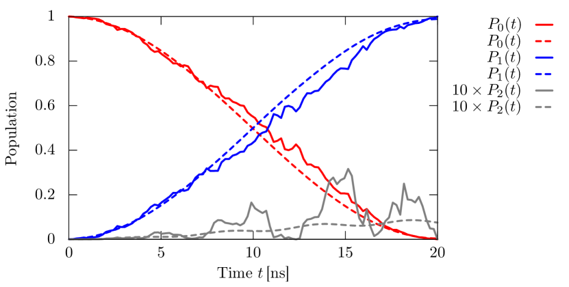
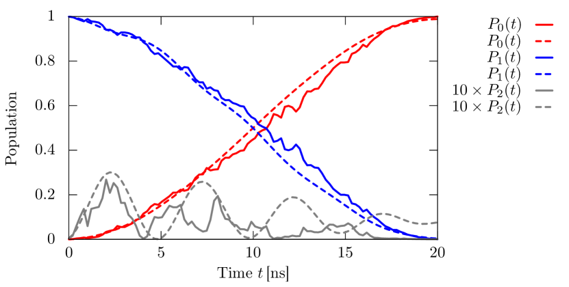
Figure 3: Populations of a qutrit starting in the ground (top panel) and excited (bottom panel) state for the optimized sequence (solid lines) and the initial sequence (dashed lines). The population of the leakage level is enhanced by a factor of 10 for better legibility. The algorithm suppresses leakage to the ending gate time.

As gradient-based algorithms are not straightforward here, we use a genetic algorithm Whitley (1994); Sutton and Boyden (1994) to optimize the pulse sequence. This versatile tool for global optimization is a natural candidate for the problem at hand, since our pulse sequence is already encoded in a binary string. Other genetic algorithms have been applied successfully in analog quantum optimal control, e.g., to optimize laser pulses to control molecules Judson and Rabitz (1992).

Here, we search for a local minimum in the control landscape starting with the sequence described earlier Bodenhausen et al. (1976); McDermott and Vavilov (2014), and stop as soon as we reach the target fidelity. Within the genetic algorithm framework, every solution for the variational parameters of the control problem is encoded in a genome. At each iteration, a selection of genomes will be merged by a crossover of genome pairs. The new and old genomes are mutated and the genomes with the best fitness make it to the next generation. Finding the right parameters for the genetic algorithm can be difficult, but it is common practice for most optimization problems to choose a high crossover and a low mutation probability Hartmann and Rieger (2002). The parameters of our optimization are shown in Table 1.

Population size	70
Mutation probability	0.001
Crossover probability	0.9
Number of genomes to select for mating	64
Maximum allowed iterations	200 000
Target fitness	0.9999
Elitism	1

Table 1: Parameters used in the genetic algorithm. See Ref. Whitley (1994) for background.

Using that algorithm and setting our gate fidelity as a fitness measure we found the solutions for the sequence shown in Fig. 2 and for the populations shown in Fig. 3. The algorithm mainly corrects for leakage into the third energy level, which always leads to an increase in the number of pulses—in the solutions presented here, from $n=100$ to $n=301$. The time taken for a run is about 150 s and the improvement is shown in Fig. 4. We encounter a broad variation over different runs indicating the presence of an abundance of local traps. This is consistent with the common observation that, in principle, trap-free control landscape Rabitz et al. (2004) develops traps when the space of the available pulse shapes is strongly constrained.

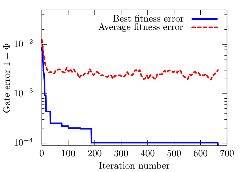
Figure 4: Starting with a sequence shown in Ref. Bodenhausen et al. (1976); McDermott and Vavilov (2014), genetic algorithms are used for optimization. At each iteration, a new population of different pulse sequences is created from their parents, while the best solution of a generation with the lowest fidelity error is kept until either the algorithm finds a better one or a given threshold is exceeded.

IV Quantum speed limit

With the genetic algorithm at hand, we can search for shorter gate times $t_{\textrm{gate}}$ for the Pauli-$Y$ gate. We keep the widths of the pulses constant, which decreases the number of pixels with a decreasing gate time. The reachable fidelities are shown in Fig. 5. The shortest possible gate time we could find within the genetic algorithm is $t_{\textrm{gate}}=6$ ns. Each optimization stops if a fidelity $>0.9999$ is reached or the maximum number of iterations (200 000) is exceeded. We point out that, for short gate times, the evenly spaced pulse sequence is no longer a viable solution if we do not have any control of the pulse amplitude.

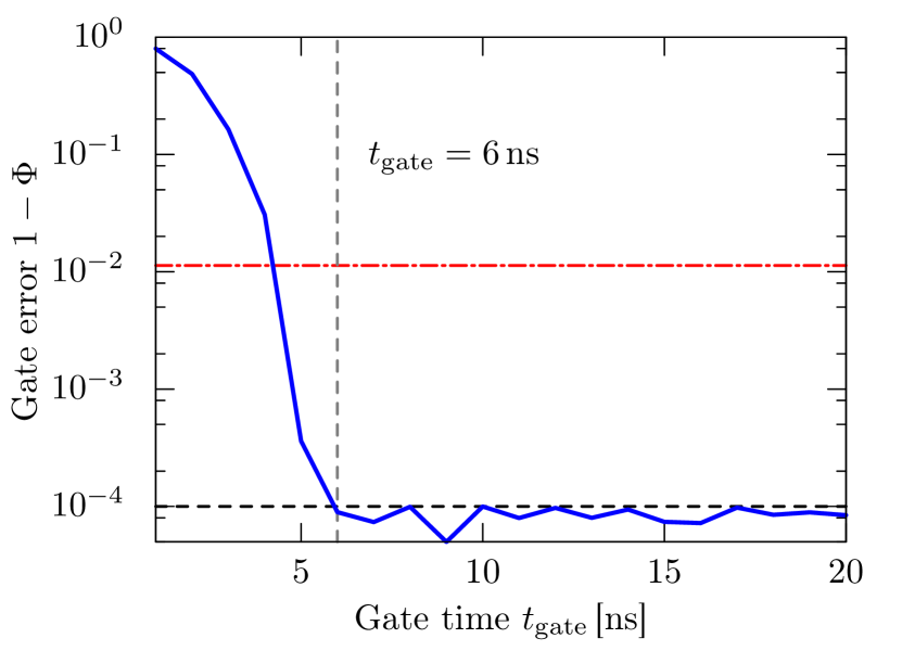
Figure 5: The gate errors of the optimizations for different gate times. The widths of the pulses have been kept constant; i.e., the number of pixels changes with the gate time linearly. The horizontal red dash-dotted line is the fidelity error of the initial sequence for 20 ns, and the horizontal black dashed line indicates the stopping condition of the algorithm when a fidelity $>0.9999$ has been reached.

V Timing errors

So far the clock has been assumed to be a perfect one. Here, we take inevitable timing errors into account, that lead to small pulse delays Rylyakov and Likharev (1999) and, therefore, to deviations from the optimal fidelity. We simulate timing errors by multiplying every applied pulse $\boldsymbol{U}_{1}$ in the optimized sequence with a free-evolution operator of a time interval $\delta t$ from the right, and its adjoint from the left. Therefore, a positive $\delta t$ indicates a pulse which arrives with a delay, and a negative $\delta t$ indicates that the pulse arrives earlier:

$$\boldsymbol{U}_{1}^{\prime}=\boldsymbol{U}_{0}(-\delta t)\boldsymbol{U}_{1}\boldsymbol{U}_{0}(\delta t)\,.$$ (9)

$\delta t$ is a normal distributed random time with standard deviation $\sigma$ for external jitter and $\sqrt{k}\sigma$ for internal jitter, where $k$ is the applied pulse number. For each value of $\sigma$, the fidelity of the time evolution has been averaged over 1000 runs for the optimized sequence. As can be obtained from Fig. 6, the external clocking scheme is more robust by an order of magnitude of the standard deviation. It is still within the target fidelity when the jitter time scale is 10 % of the pulse width, while, for an internal clock it is around 1 %. If the jitter time reaches the pulse duration, the gate error is still on the same scale as where we started our optimization. We therefore conclude that an external clock should be used in favor of an internal one for future devices.

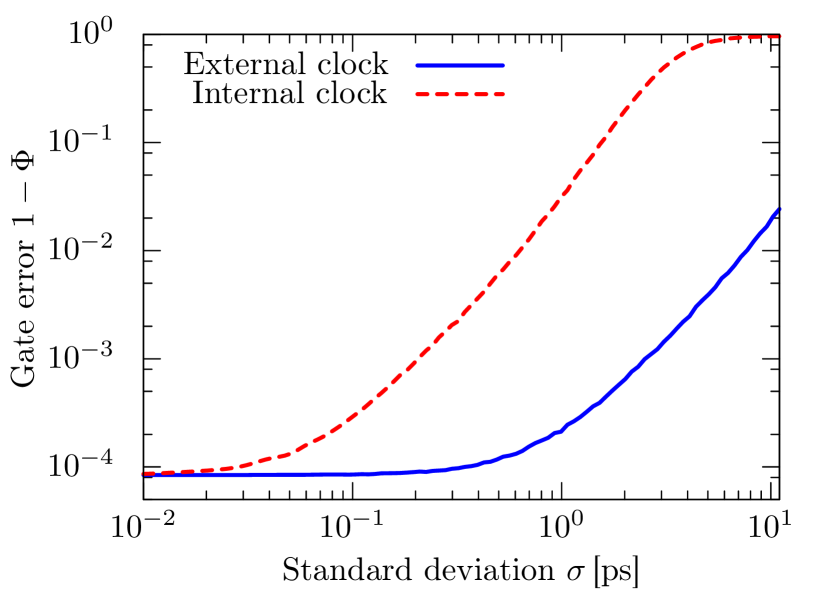
Figure 6: The gate error of the optimized sequence for timing jitters with constant variance (external clock) and linear growing variance (internal clock). The gate errors have been averaged over 1000 runs of the time evolution for each value of $\sigma$.

VI Conclusion

We successfully develop and apply an optimal-control method for pulses with only a single bit of amplitude resolution. Finding the right binary string leads to minimization of the leakage error in the transmon system, and thus gate-control precision compatible with the requirements of fault-tolerant quantum computing. The results presented here show a fidelity improvement of several orders of magnitude over equal pulse-spacing sequences while being robust under external timing jitter. RSFQ shift registers are needed to perform the optimized sequence and are an essential part of on-chip SFQ-qubit control. This makes the underlying SFQ-pulse platform together with the single-bit optimal-control theory a possible and attractive candidate for an integrated control layer in a quantum processor.

References

- Likharev and Semenov (1991) K. K. Likharev and V. K. Semenov, “RSFQ logic/memory family: a new Josephson-junction technology for sub-terahertz-clock-frequency digital systems,” IEEE Trans. Appl. Supercond. 1, 3–28 (1991).
- Likharev (2012) K. K. Likharev, “Superconductor digital electronics,” Physica C Supercond. 482, 6–18 (2012).
- Castellano et al. (2007) Maria Gabriella Castellano, Fabio Chiarello, Roberto Leoni, Guido Torrioli, Pasquale Carelli, Carlo Cosmelli, Marat Khabipov, Alexander B. Zorin, and Dmitri Balashov, “Rapid single-flux quantum control of the energy potential in a double SQUID qubit circuit,” Supercond. Sci. Technol. 20, 500 (2007).
- Orlando et al. (2002) T. P. Orlando, S. Lloyd, L. S. Levitov, K. K. Berggren, M. J. Feldman, M. F. Bocko, J. E. Mooij, C. J. P. Harmans, and C. H. van der Wal, “Flux-based superconducting qubits for quantum computation,” Physica C Supercond. 372–376, 194–200 (2002).
- Feldman and Bocko (2001) Marc J. Feldman and Mark F. Bocko, “A realistic experiment to demonstrate macroscopic quantum coherence,” Physica C Supercond. 350, 171–176 (2001).
- Ohki et al. (2007) Thomas A. Ohki, Michael Wulf, and Marc J. Feldman, “Low-Jc rapid single flux quantum (RSFQ) qubit control circuit,” IEEE Trans. Appl. Supercond. 17, 154–157 (2007).
- Semenov and Averin (2003) Vasili K. Semenov and Dmitri V. Averin, “SFQ control circuits for josephson junction qubits,” IEEE Trans. Appl. Supercond. 13, 960–965 (2003).
- Fedorov et al. (2007) Arkady Fedorov, Alexander Shnirman, Gerd Schön, and Anna Kidiyarova-Shevchenko, “Reading out the state of a flux qubit by josephson transmission line solitons,” Phys. Rev. B 75, 224504 (2007).
- Fedorov et al. (2014) Kirill G. Fedorov, Anastasia V. Shcherbakova, Michael J. Wolf, Detlef Beckmann, and Alexey V. Ustinov, “Fluxon readout of a superconducting qubit,” Phys. Rev. Lett. 112, 160502 (2014).
- Ohki et al. (2005) Thomas A. Ohki, Michael Wulf, and Mark F. Bocko, “Picosecond on-chip qubit control circuitry,” IEEE Trans. Appl. Supercond. 15, 837–840 (2005).
- Gaj et al. (1997) Kris Gaj, Eby G. Friedman, and Marc J. Feldman, “Timing of multi-gigahertz rapid single flux quantum digital circuits,” J. VLSI Signal Process. Syst. Signal Image Video Technol. 16, 247–276 (1997).
- McDermott and Vavilov (2014) R. McDermott and M. G. Vavilov, “Accurate qubit control with single flux quantum pulses,” Phys. Rev. Applied 2, 014007 (2014).
- Fowler et al. (2012) Austin G. Fowler, Matteo Mariantoni, John M. Martinis, and Andrew N. Cleland, “Surface codes: Towards practical large-scale quantum computation,” Phys. Rev. A 86, 032324 (2012).
- Mukhanov (1993) Oleg A. Mukhanov, “Rapid single flux quantum (RSFQ) shift register family,” IEEE Trans. Appl. Supercond. 3, 2578–2581 (1993).
- Glaser et al. (2015) Steffen J. Glaser, Ugo Boscain, Tommaso Calarco, Christiane P. Koch, Walter Köckenberger, Ronnie Kosloff, Ilya Kuprov, Burkard Luy, Sophie Schirmer, Thomas Schulte-Herbrüggen, D. Sugny, and Frank K. Wilhelm, “Training Schrödinger’s cat: quantum optimal control,” Eur. Phys. J. D 69, 279 (2015).
- Motzoi et al. (2009) F. Motzoi, J. M. Gambetta, P. Rebentrost, and F. K. Wilhelm, “Simple pulses for elimination of leakage in weakly nonlinear qubits,” Phys. Rev. Lett. 103, 110501 (2009).
- Schutjens et al. (2013) R. Schutjens, F. A. Dagga, D. J. Egger, and F. K. Wilhelm, “Single-qubit gates in frequency-crowded transmon systems,” Phys. Rev. A 88, 052330 (2013).
- Egger and Wilhelm (2014) D. J. Egger and F. K. Wilhelm, “Adaptive hybrid optimal quantum control for imprecisely characterized systems,” Phys. Rev. Lett. 112, 240503 (2014).
- Koch et al. (2007) Jens Koch, Terri M. Yu, Jay Gambetta, A. A. Houck, D. I. Schuster, J. Majer, Alexandre Blais, M. H. Devoret, S. M. Girvin, and R. J. Schoelkopf, “Charge-insensitive qubit design derived from the Cooper pair box,” Phys. Rev. A 76, 042319 (2007).
- Girvin (2011) Steven M. Girvin, “Circuit QED: Superconducting qubits coupled to microwave photons,” in Quantum Machines: Measurement and Control of Engineered Quantum Systems (Oxford University Press, 2011).
- Rebentrost and Wilhelm (2009) P. Rebentrost and F. K. Wilhelm, “Optimal control of a leaking qubit,” Phys. Rev. B 79, 060507 (2009).
- Bodenhausen et al. (1976) Geoffrey Bodenhausen, Ray Freeman, and Gareth A. Morris, “A simple pulse sequence for selective excitation in Fourier transform NMR,” J. Magn. Reson. 23, 171–175 (1976).
- Whitley (1994) Darrell Whitley, “A genetic algorithm tutorial,” Stat. Comput. 4, 65–85 (1994).
- Sutton and Boyden (1994) Patrick Sutton and Sheri Boyden, “Genetic algorithms: A general search procedure,” Am. J. Phys. 62, 549–552 (1994).
- Judson and Rabitz (1992) R. S. Judson and H. Rabitz, “Teaching lasers to control molecules,” Phys. Rev. Lett. 68, 1500–1503 (1992).
- Hartmann and Rieger (2002) Alexander K. Hartmann and Heiko Rieger, Optimization Algorithms in Physics (Wiley-VCH, Weinheim, 2002).
- Rabitz et al. (2004) Herschel A. Rabitz, Michael M. Hsieh, and Carey M. Rosenthal, “Quantum optimally controlled transition landscapes,” Science 303, 1998–2001 (2004).
- Rylyakov and Likharev (1999) A. V. Rylyakov and K. K. Likharev, “Pulse jitter and timing errors in RSFQ circuits,” IEEE Trans. Appl. Supercond. 9, 3539–3544 (1999).