H₂ distribution during the formation of multiphase molecular clouds

Abstract

Context. H₂ is the simplest and the most abundant molecule in the interstellar medium (ISM), and its formation precedes the formation of other molecules.

Aims. Understanding the dynamical influence of the environment and the interplay between the thermal processes related to the formation and destruction of H₂ and the structure of the cloud is mandatory to understand correctly the observations of H₂.

Methods. We performed high-resolution magnetohydrodynamical colliding-flow simulations with the adaptive mesh refinement code RAMSES in which the physics of H₂ has been included. We compared the simulation results with various observations of the H₂ molecule, including the column densities of excited rotational levels.

Results. As a result of a combination of thermal pressure, ram pressure, and gravity, the clouds produced at the converging point of HI streams are highly inhomogeneous. H₂ molecules quickly form in relatively dense clumps and spread into the diffuse interclump gas. This in particular leads to the existence of significant abundances of H₂ in the diffuse and warm gas that lies in between clumps. Simulations and observations show similar trends, especially for the HI-to-H₂ transition (H₂ fraction vs total hydrogen column density). Moreover, the abundances of excited rotational levels, calculated at equilibrium in the simulations, turn out to be very similar to the observed abundances inferred from FUSE results. This is a direct consequence of the presence of the H₂ enriched diffuse and warm gas.

Conclusions. Our simulations, which self-consistently form molecular clouds out of the diffuse atomic gas, show that H₂ rapidly forms in the dense clumps and, due to the complex structure of molecular clouds, quickly spreads at lower densities. Consequently, a significant fraction of warm H₂ exists in the low-density gas. This warm H₂ leads to column densities of excited rotational levels close to the observed ones and probably reveals the complex intermix between the warm and cold gas in molecular clouds. This suggests that the two-phase structure of molecular clouds is an essential ingredient for fully understanding molecular hydrogen in these objects.

1 Introduction

It is well known that stars form in dense and self-gravitating molecular clouds and that the star formation rate per unit area ($\Sigma_{\mathrm{SFR}}$) is on average relatively well correlated with the H₂ surface density ($\Sigma_{\mathrm{H_{2}}}$) (Leroy et al. 2013; Lada et al. 2012; Wong & Blitz 2002; Bigiel et al. 2008).

Although H₂ is the simplest and most abundant molecule in the interstellar medium (ISM), it is very hard to observe directly. Because of its homonuclear nature, H₂ lacks a permament dipole and only weak quadrupolar transitions are allowed. Moreover, excitation energies are very high and require very high temperatures or strong ultraviolet (UV) fields to excite its rotational levels (Kennicutt & Evans 2012). H₂ can be observed in emission by infrared (IR) rovibrational transitions (Burton et al. 1992; Santangelo et al. 2014; Habart et al. 2011), or in absorption at far-ultraviolet (far-UV) wavelengths from the Lyman and Werner bands. These bands were first observed by Spitzer & Jenkins (1975) using the Copernicus satellite. The Far Ultraviolet Spectroscopic Explorer (FUSE) (Moos et al. 2000) offered new perspectives on the study of H₂ in the ISM through its sensitivity, which is $10^{5}$ times higher than Copernicus in the far-UV part of the spectrum, providing measurements of H₂ column densities (of the total column density of H₂ and for several rotational levels $J$) along translucent lines of sight (Wakker 2006; Sheffer et al. 2008).

While it seems to be clear that molecular gas is well correlated with star formation at different scales, it is still an open question how the gas becomes molecular. Since understanding the atomic-to-molecular hydrogen (HI-to-H₂) transition is of the highest importance for understanding the star-forming process, numerous models have been developed (e.g. Krumholz et al. 2008; Sternberg et al. 2014) and seem able to reproduce many of the observed constraints. While extremely useful, these models leave aside the dynamical aspects of H₂ formation. In particular, the question of the relatively long timescale that is needed to form the H₂ molecules has for many years been difficult to reconcile with short-lived and quickly forming molecular clouds. The typical timescale for H₂ formation is of the order of $10^{9}{\rm yr}/n$ (Hollenbach et al. 1971), which would lead to ages older than 10 Myr for molecular clouds of mean densities of the order of 10-100 cm^-3 (Blitz & Shu 1980). However, Glover & Mac Low (2007a) and Glover & Mac Low (2007b), who have simulated the formation of molecular hydrogen in supersonic clouds, showed that H₂ can form relatively quickly in the dense clumps induced by the shocks, leading to a significantly shorter timescale (typically of about 3 Myr). Recently, Micic et al. (2012) explored the influence of the turbulent forcing and showed that it has a significant influence on the timescale of H₂ formation. This is because compressible forcing leads to denser clumps than solenoidal forcing, for which the motions are less compressible. This clearly shows that dynamics is playing an important role in the process of HI-to-H₂ transition, at least at the scale of a molecular cloud.

In the Milky Way most of the molecular hydrogen is in the form of low-temperature gas, but different observations have brought to light the existence of large amounts of fairly warm H₂ in the ISM (Valentijn & van der Werf 1999; Verstraete et al. 1999). Gry et al. (2002) and Lacour et al. (2005) have shown that the H₂ excitation resulting from UV pumping and from H₂ formation cannot account for the observed population of H₂ excited levels ($J>2$). Excited H₂ is likely explained by the presence of a warm and turbulent layer associated with the molecular cloud. But in such warm gas, which is characterised by very low densities ($n_{\mathrm{H}}\approx 1-10\leavevmode\nobreak\ \mathrm{cm^{-3}}$) and very high temperatures ($T\approx 10^{3}-10^{4}\leavevmode\nobreak\ \mathrm{K}$), H₂ formation on grain surfaces becomes negligible, which accordingly leads to an apparent contradiction. Recently, Godard et al. (2009) have investigated the possibility that warm H₂ could form during intermittent high-energy dissipation events such as vortices and shocks. They showed in particular that under plausible assumptions for the distributions of these events, the observed abundance of excited H₂ molecules could be reproduced. Another possibility to explain the abundance of these excited H₂ molecules is that they could be formed in dense gas and then be transported in more diffuse and warmer medium. This possibility has been investigated by Lesaffre et al. (2007) using a 1D model and a prescription to take into account the turbulent diffusion between the phases. In particular, they found that the abundance of H₂ molecules at low density and high temperature increases with the turbulent diffusion efficiency.

While different in nature, previous works (Glover & Mac Low 2007a, b; Lesaffre et al. 2007; Godard et al. 2009) therefore consistently found that the formation of H₂ is significantly influenced by the dynamics of the flow in which it forms. Although the exact mechanism that leads to the formation of molecular clouds is still under investigation, it seems unavoidable to consider converging streams of diffuse gas (e.g. Hennebelle & Falgarone 2012; Dobbs et al. 2014). What exactly triggers these flows is not fully elucidated yet but is most likely due a combination of gravity, large-scale turbulence, and large-scale shell expansion. Another important issue is the thermodynamical state of the gas. The diffuse gas out of which molecular clouds form is most likely a mixture of phases made of warm and cold atomic hydrogen (HI) and even possibly somewhat diffuse molecular gas. Such a multiphase medium presents strong temperature variations (typically from 8000 K to lower than 50 K). This causes the dynamics of the flow to be significantly different from isothermal or nearly isothermal flow (see Audit & Hennebelle 2010, for a comparison between barotropic and two-phase flows). Moreover, the two-phase nature of the diffuse atomic medium has been found to persist in molecular clouds (Hennebelle et al. 2008; Heitsch et al. 2008a; Banerjee et al. 2009; Vázquez-Semadeni et al. 2010; Inoue & Inutsuka 2012). This in particular produces a medium in which supersonic clumps of cold gas are embedded in a diffuse phase of subsonic warm gas. Consequently, the question about the consequences of the multiphase nature of a molecular cloud are for the formation of H₂. Clearly, various processes may occur. First of all, the dense clumps are continuously forming and accreting out of the diffuse gas because molecular clouds continue to accrete. Second, some of the H₂ formed at high density is likely to be spread in low-density high-temperature gas because of the phase exchanges.

We here present numerical simulations using a simple model for H₂ formation within a dynamically evolving turbulent molecular cloud that is formed through colliding streams of atomic gas. Such flows, sometimes called colliding flows, have been widely used to study the formation of molecular clouds because they represent a good compromise between the need to assemble the diffuse material from the large scales and the need to accurately describe the small scales within the molecular clouds (Hennebelle & Pérault 1999; Ballesteros-Paredes et al. 1999; Heitsch et al. 2006; Vázquez-Semadeni et al. 2006; Clark et al. 2012). The content of this paper is as follows: in Sect. 2 we present the governing equations and the physical processes, such as H₂ formation. In Sect. 3 we describe the numerical setup that we use to perform the simulations. In Sect. 4 we present the results of our simulations, first describing the general structure of the cloud and then focussing on the H₂ distribution. We perform a few complementary calculations that aim at better understanding the physical mechanisms at play in the simulations. Then in Sect. 5 we compare our results with various observations that have quantified the abundance of H₂ and find very reasonable agreements. Finally, we summarise and discuss the implications of our work in Sect. 6.

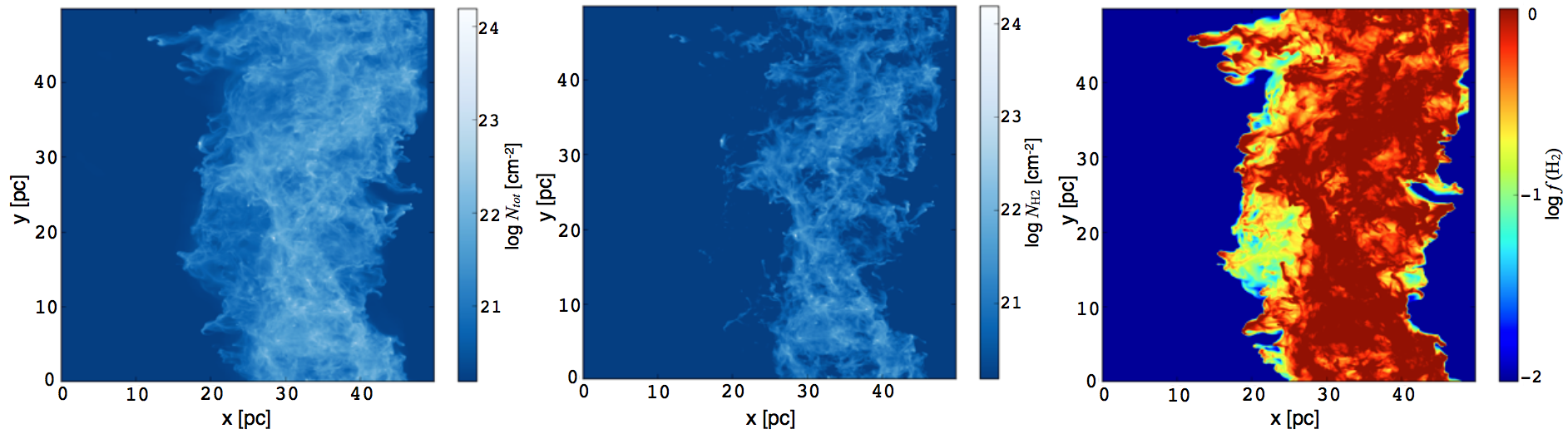
Figure 1: Column density maps. Total hydrogen column density map (left), H₂ column density map (centre), and molecular fraction (right). The gas enters the box from both sides ($x$-axis), and the conditions for the other sides are periodic. The gas is compressed along the $x$-direction and the cloud forms toward the middle of the box.

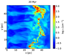
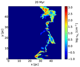
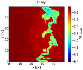
Figure 2: Slices cut through the mid-plane. The panel on the left shows the total number density of hydrogen nucleons, the panel in the centre shows the number density of molecular hydrogen (on the same scale), and the panel on the right shows the mean shielding factor for the H₂ photodissociation rate coefficient, calculated as $\langle\exp(-\tau_{d,1000})f_{\mathrm{shield}}\rangle$.

2 Physical processes

2.1 Governing fluid equations

We consider the usual compressive magnetohydrodynamical equations that govern the behaviour of the gas. These equations written in their conservative form are

$$\frac{\partial\rho}{\partial t}+\nabla\cdot(\rho\mathbf{v}) = 0,$$ (1)

$$\frac{\partial\rho\mathbf{v}}{\partial t}+\nabla\cdot(\rho\mathbf{v}\mathbf{v}-\mathbf{B}\mathbf{B})+\nabla P = -\rho\nabla\phi,$$ (2)

$$\frac{\partial E}{\partial t}+\nabla\cdot[(E+P)\mathbf{v}-\mathbf{B}(\mathbf{B}\mathbf{v})] = -\rho{\cal L},$$ (3)

$$\frac{\partial\mathbf{B}}{\partial t}+\nabla\cdot(\mathbf{v}\mathbf{B}-\mathbf{B}\mathbf{v}) = 0,$$ (4)

$$\nabla^{2}\phi = 4\pi G\rho,$$ (5)

where $\rho$, $\mathbf{v}$, $\mathbf{B}$, $P$, $E$, and $\phi$ are the mass density, velocity field, magnetic field, total energy, and the gravitational potential of the gas, respectively, and $\cal L$ is the net loss function that describes gas cooling and heating.

2.2 Chemistry of H₂

The fluid equations (Eqs. 1-5) are complemented by an equation that describes the formation of the H₂ molecules,

$$\frac{\partial n_{\mathrm{H_{2}}}}{\partial t}+\nabla\cdot(n_{\mathrm{H_{2}}}\mathbf{v}) = k_{\mathrm{form}}n(n-2n_{\mathrm{H_{2}}})-k_{\mathrm{ph}}n_{\mathrm{H_{2}}},$$ (6)

where $n$ is the total hydrogen density, $n_{\mathrm{H_{2}}}$ represents the density of H₂, and $k_{\mathrm{form}}$ and $k_{\mathrm{ph}}$ represent the formation and destruction rates of H₂.

2.2.1 H₂ formation

When two hydrogen atoms encounter each other in the gas phase, they cannot radiate the excess of energy because of the lack of an electric dipole moment, and therefore H₂ formation in the gas phase is negligible. It is widely accepted today that H₂ is formed through grain catalysis (Hollenbach & Salpeter 1971; Gould & Salpeter 1963). Hydrogen atoms can adsorb onto the grain surfaces and encounter another hydrogen atom to form a H₂ molecule through two mechanisms: the Langmuir-Hinshelwood mechanism, where atoms are physisorbed (efficient in shielded gas), and the Eley-Rideal mechanism, or chemisorption (efficient on warm grains) (Le Bourlot et al. 2012; Bron et al. 2014). The detailed physical description of these two mechanisms is complex and the numerical treatment is computationally expensive. For this reason we adopted a simpler description for H₂ formation on grain surfaces, given by the following mean formation rate:

$$k_{\mathrm{form,0}}=3\times 10^{-17}\leavevmode\nobreak\ \mathrm{cm^{3}s^{-1}}.$$ (7)

This rate was first derived by Jura (1974), using Copernicus observations, and was confirmed by Gry et al. (2002) using FUSE observations. The formation rate depends on the local gas temperature and on the adsorption properties of the grain, therefore this value is corrected for by the dependence on temperature and by a sticking coefficient:

$$k_{\mathrm{form}}=k_{\mathrm{form,0}}\sqrt{\frac{T}{100\ \mathrm{K}}}\times S(T).$$ (8)

$S(T)$ is the empirical expression for the sticking coefficient of hydrogen atoms on the grain surface as described in Le Bourlot et al. (2012),

$$S(T)=\frac{1}{1+\left(\frac{T}{T_{2}}\right)^{\beta}},$$ (9)

where we use the same fitting values as Bron et al. (2014), namely $T_{2}=464\leavevmode\nobreak\ \mathrm{K}$, and $\beta=1.5$.

2.2.2 H₂ destruction

The main mechanism that destroys the H₂ molecule is photodissociation by absorption of UV photons in the $912$ - $1100$ $\mathrm{\SIUnitSymbolAngstrom}$ range (Lyman and Werner transitions). In a UV field of strength $G_{0}$, H₂ is photodissociated in optically thin gas at a rate (Draine & Bertoldi 1996) of

$$k_{\mathrm{ph,0}}=3.3\times 10^{-11}G_{0}\ \mathrm{s^{-1}},$$ (10)

but the H₂ gas can protect itself against photodissociation by two shielding effects. The first shielding effect is the continuous dust absorption, while the second effect is the line absorption due to other H₂ molecules, called self-shielding. Draine & Bertoldi (1996) showed that the photodissociation rate can be written as

$$k_{\mathrm{ph}}=e^{-\tau_{d,1000}}f_{\mathrm{shield}}(\mathcal{N}_{\mathrm{H_{2}}})k_{\mathrm{ph,0}}.$$ (11)

The first term is the effect of the dust. Here $\tau_{d,1000}=\sigma_{d,1000}\mathcal{N}_{tot}$ is the optical depth along a line of sight ($\sigma_{d,1000}=2\times 10^{-21}\mathrm{cm^{-2}}$ is the effective attenuation cross section for dust grains at $\lambda=1000\ \mathrm{\SIUnitSymbolAngstrom}$ and $\mathcal{N}_{tot}$ is the total column density of hydrogen). The second term is the self-shielding factor, and we use the same approximation,

$$f_{\mathrm{shield}}=\frac{0.965}{(1+x/b_{5})^{2}}+\frac{0.035}{(1+x)^{1/2}}\mathrm{exp}(-8.5\times 10^{-4}(1+x)^{1/2}),$$ (12)

where $x=\mathcal{N}_{\mathrm{H_{2}}}/5\times 10^{14}\leavevmode\nobreak\ \mathrm{cm^{-2}}$, $b_{5}=b/10^{5}\leavevmode\nobreak\ \mathrm{cm\ s^{-1}}$, where $b$ is the Doppler-broadening parameter, which is typically $2\leavevmode\nobreak\ \mathrm{km\ s^{-1}}$, but it can reach values as high as $10\leavevmode\nobreak\ \mathrm{km\ s^{-1}}$ (Shull et al. 2000). We assume that the turbulent contribution dominates, then we use $b=2\leavevmode\nobreak\ \mathrm{km\ s^{-1}}$ (see Appendix B for the influence of this choice on the shielding coefficient).

2.3 Thermal processes

For the heating and cooling of the gas, we used the same treatment as we did previously (Valdivia & Hennebelle 2014) (see also Audit & Hennebelle 2005), which we describe in this section and call the standard heating and cooling, to which we have added the thermal feedback from H₂, described in Sect. 2.3.1.

The dominant heating process in the gas is due to the ultraviolet flux from the interstellar radiation field (ISRF) through the photoelectric effect on grains (Bakes & Tielens 1994; Wolfire et al. 1995), where we use the effective UV field strength, calculated using our attenuation factor $\chi$ for the UV field. We also include the heating by cosmic rays (Goldsmith 2001), which is important in well shielded regions.

The primary coolant at low temperature is the ${}^{2}P_{3/2}\rightarrow\ ^{2}P_{1/2}$ [CII] fine-structure transition at $158\leavevmode\nobreak\ \mathrm{\mathrm{\SIUnitSymbolMicro}m}$ (Launay & Roueff 1977; Hayes & Nussbaumer 1984; Wolfire et al. 1995). At higher temperature, fine-structure levels of OI can be excited and thus contribute to the cooling of the gas. We include the [OI] $63\leavevmode\nobreak\ \mathrm{\mathrm{\SIUnitSymbolMicro}m}$ and $146\leavevmode\nobreak\ \mathrm{\mathrm{\SIUnitSymbolMicro}m}$ line emission (Flower et al. 1986; Tielens 2005; Wolfire et al. 2003). For the Lyman $\alpha$ emission, which becomes dominant at high temperatures, we use the classical expression of Spitzer (1978). We also include the cooling by electron recombination onto dust grains using the prescription of Wolfire et al. (1995, 2003) and Bakes & Tielens (1994). We note that strictly speaking, this cooling function does not include molecular cooling in spite of the high densities reached in the simulation. However, it leads to temperatures that are entirely reasonable even at high densities and therefore appears to be sufficiently accurate, in particular because we are not explicitly solving for the formation of molecules in addition to H₂ (see Levrier et al. 2012, for a quantitative estimate).

2.3.1 Thermal feedback from H₂

To the atomic cooling, described before, we added the molecular cooling by H₂ lines and the heating by H₂ formation and destruction.
During the H₂ formation process, about $4.5\leavevmode\nobreak\ \mathrm{eV}$ are released. The distribution of this energy into translational energy, H₂ internal energy (rotational and vibrational excitation), and into the grain heating is not well known, and the derived fraction of this energy that actually heats the gas varies from one author to another (Le Bourlot et al. 2012; Glover & Mac Low 2007a). We consider an equipartition of the energy, which means that one-third of the energy released goes into heating the gas,

$$\Gamma_{\mathrm{form}}=2.4\times 10^{-12}k_{\mathrm{form}}n_{\mathrm{H}}n\ \mathrm{erg\ s^{-1}cm^{-3}}.$$ (13)

H₂ photodissociation provides an additional heating source. Following Black & Dalgarno (1977) and Glover & Mac Low (2007a), we assumed $0.4\ \mathrm{eV}$ released into the gas per photodissociation,

$$\Gamma_{\mathrm{ph}}=6.4\times 10^{-13}k_{\mathrm{ph}}n_{\mathrm{H_{2}}}\ \mathrm{erg\ s^{-1}cm^{-3}}.$$ (14)

H₂ contributes to the cooling of the gas through line emission and can become strong for the diffuse medium under certain conditions (Glover & Clark 2014; Gnedin & Kravtsov 2011). As H₂ is a homonuclear molecule, only quadrupolar transitions are allowed, and thus, the ortho and para states can be treated independently. In our simulations we adopted the cooling function from Le Bourlot et al. (1999). This is a function of temperature, total density, $n(\mathrm{HI})/n(\mathrm{H_{2}})$ relative abundance, and of the ortho-to-para-H₂ ratio (OPR). It considers transitions between the first $51$ rovibrational energy levels. As the cooling function is quite insensitive to the OPR, we fixed it to 3 for simplicity.

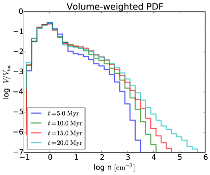
Figure 3: Density PDF evolution. Colour lines show the density PDF at $t=5$ (blue), $10$ (green), $15$ (red), and $20$ Myr (light blue).

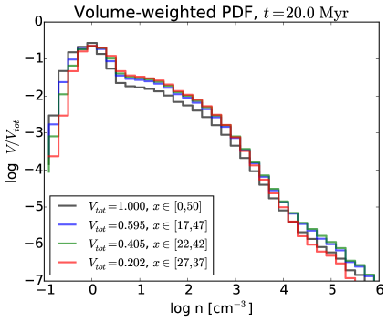
Figure 4: Volume filling factor as a function of density in different regions. $V_{tot}$ is the volume fraction of each region.

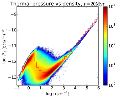
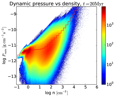
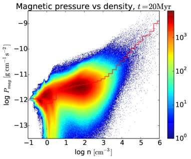
Figure 5: Different pressures in the ISM vs density. The top panel shows the thermal pressure, $P_{th}=nkT$, the middle panel the ram pressure, $P_{ram}=\rho V^{2}$, and the bottom panel the magnetic pressure, $P_{mag}=B^{2}/8\pi$ in the simulation box. The red line shows the mean value per density bin. The colour scale indicates the number of points.

Figure 6: Statistics of clumps. The top panel shows the mass spectrum, the second panel their internal velocity dispersion as a function of size, the third panel the kinetic $\beta=P_{ram}/P_{mag}$ , and the bottom panel displays the H₂ fraction as a function of mass.

3 Numerical setup and initial conditions

As already discussed, colliding flows are a practical ansatz to gather matter to form a molecular cloud (Inoue & Inutsuka 2012; Audit & Hennebelle 2005; Vázquez-Semadeni et al. 2007; Heitsch et al. 2005, 2006, 2008b; Micic et al. 2013) to mimic large-scale converging flows, as in Galactic spiral arms or in super-bubble collisions.

3.1 General setup

The setup is very similar to the one that Valdivia & Hennebelle (2014) used. The size of the simulation box is $L=50\leavevmode\nobreak\ \mathrm{pc}$ and it is initially uniformly filled with atomic gas, with initial number density $n_{\mathrm{tot}}=1\leavevmode\nobreak\ \mathrm{cm^{-3}}$ and initial temperature $T=8000\leavevmode\nobreak\ \mathrm{K}$. Atomic gas, with the same number density and temperature, is injected from the left and right sides of the box with an average velocity $V_{0}=15\leavevmode\nobreak\ \mathrm{km\ s^{-1}}$, aligned with the $x$-axis, which is modulated by a function of amplitude $\epsilon=0.5$, producing a slightly turbulent profile, as in Audit & Hennebelle (2005). We use periodic boundary conditions for the remaining sides. The gas is initially uniformly magnetised, with a moderate magnetic field ($\sim 2.5\leavevmode\nobreak\ \mathrm{\mathrm{\SIUnitSymbolMicro}G}$) aligned with the inflowing gas. This configuration avoids boundary issues and facilitates the building of the cloud. Introducing an angle between the magnetic and the velocity fields would be more realistic, but this very simplified framework requires relatively small angles (Hennebelle & Pérault 2000; Körtgen & Banerjee 2015; Inoue & Inutsuka 2012).

3.2 Radiative transfer and dust shielding

Molecular clouds are embedded in the interstellar radiation field (ISRF), which is assumed to be isotropic and constant throughout the space (Habing 1968). The whole simulation is embedded in an external and isotropic UV field that is assumed to be monochromatic, of strength $G_{0}=1.7$ in Habing units, and which heats the gas. UV photons are assumed to enter the computational box from all directions and undergo interactions with dust grains in their pathways before reaching any cell. The intensity of the UV field varies from one point to another according to the dust shielding factor $\chi$, which is calculated at each point of the simulation box for each timestep using our tree-based method, which is fully described in Valdivia & Hennebelle (2014). Hence, the strength of the local UV field, after dust shielding, can be written $\overline{G}_{0}\leavevmode\nobreak\ =\leavevmode\nobreak\ \chi G_{0}$, where $\chi=\langle e^{-2.5\mathrm{A_{V}}}\rangle=\langle e^{-1.3\times 10^{-21}\mathcal{N}_{\mathrm{tot}}}\rangle$, is the mean shielding factor due to dust. This mean value is calculated using a fixed number of directions. In our previous work (Valdivia & Hennebelle 2014) we have shown that the number of directions is not crucial for the dynamical evolution of the cloud. For simplicity and numerical efficiency, we therefore used 12 directions ($M=3$ intervals for the polar angle and $N=4$ for the azimuthal angle), which has turned out to be an excellent compromise between accuracy and efficiency.

We adapted the code to also compute the self-shielding (stated by Eq. 12). More precisely, along each direction we computed not only the total gas density, but also the H₂ column density from which we computed the shielding coefficient, $f_{\mathrm{shield}}$, and the extinction due to dust, $\tau_{d,1000}$. Since the UV flux is assumed to be isotropic, the final photodissociation rate is obtained by taking the mean value over all directions. We define $\chi_{\rm shield}$ as

$$\chi_{\rm shield}={k_{\mathrm{ph}}\over k_{\mathrm{ph,0}}}=\langle e^{-\tau_{d,1000}}f_{\mathrm{shield}}(\mathcal{N}_{\mathrm{H_{2}}})\rangle.$$ (15)

3.3 Numerical resolution and runs performed

To perform our simulations we employed the adaptive mesh refinement code RAMSES (Teyssier 2002; Fromang et al. 2006). RAMSES solves the MHD equations using the HLLD Riemann solvers. It preserves the nullity of the divergence of the magnetic field thanks to the use of a staggered mesh. To solve Eq. (6), we used operator splitting, solving first for the advection (which is identical to the conservation equation) and then subcycling to solve for the right-hand side. In AMR codes the refinement is done on a cell-by-cell basis. In our simulations, the refinement criterion is the density. When a cell reaches a given density threshold, it is split into eight smaller cells, each one having the same mass and volume. The process is repeated recursively until the maximum resolution is reached. In our fiducial run, we allowed two AMR levels $\ell_{min}=8$ and $\ell_{max}=10$, leading to an equivalent numerical resolution of $1024^{3}$ cells and an effective spatial resolution of about $0.05\leavevmode\nobreak\ \mathrm{pc}$. For the first refinement level (from level $\ell=8$ to $\ell=9$) the density threshold is $n_{\mathrm{thresh}}=50\leavevmode\nobreak\ \mathrm{cm^{-3}}$ and for the next refinement, the density threshold is $n_{\mathrm{thresh}}=100\leavevmode\nobreak\ \mathrm{cm^{-3}}$. To investigate numerical convergence, a particularly crucial issue when chemistry is considered, we also performed a high-resolution run for which the resolution was doubled (that is to say, using levels from 9 to 11 with the same refinement criterion).

We ran our simulations for about 20 Myr. We note that these calculations are somewhat demanding because of the short timesteps induced by high temperatures, therefore it was not possible to run the high-resolution simulations up to this point. This run reaches up to 15 Myr. To check further for convergence, we also performed low-resolution runs (128³ and 256³ , see Appendix) that we compared with our highest resolution simulations. We also performed complementary runs in which we modified the physics of H₂ formation to better understand how H₂ is formed. More precisely, in these runs we suppressed the H₂ formation above a certain density threshold,

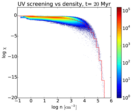
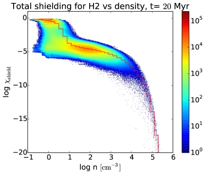
Figure 7: UV screening factor vs density (top panel) and total shielding coefficient for H₂ vs density (bottom panel) at $t=20\leavevmode\nobreak\ \mathrm{Myr}$. The red line shows the mean value per density bin, and the colour scale indicates the number of points.

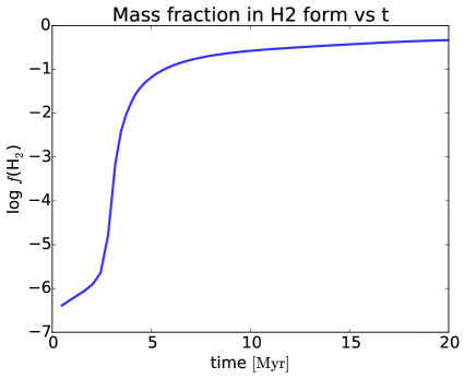
Figure 8: Evolution of the molecular fraction in the simulation box as a function of time.

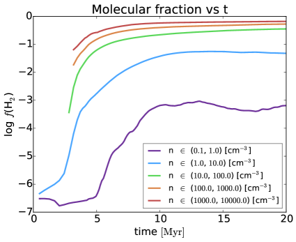
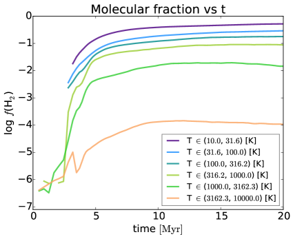
Figure 9: Molecular fraction evolution. In the top panel we show the evolution per density bin (the density increases from purple to red), in the bottom panel the evolution per temperature bin (the temperature increases from purple to salmon).

$t=5\leavevmode\nobreak\ \mathrm{Myr}$	$t=10\leavevmode\nobreak\ \mathrm{Myr}$	$t=15\leavevmode\nobreak\ \mathrm{Myr}$	$t=20\leavevmode\nobreak\ \mathrm{Myr.}$

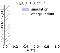
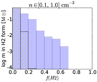
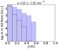
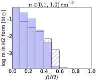
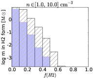
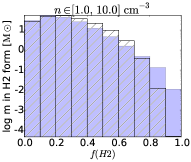
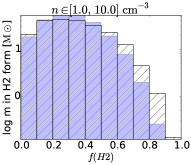
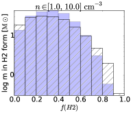
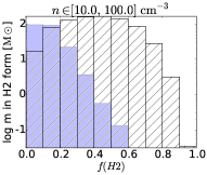
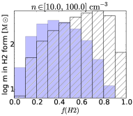
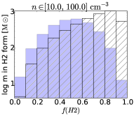
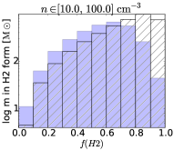
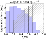
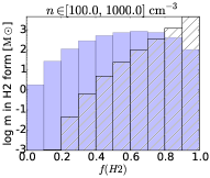
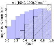
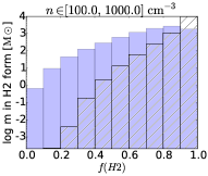
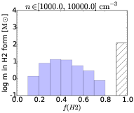
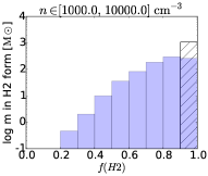
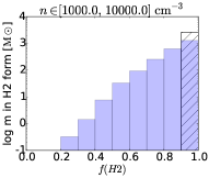
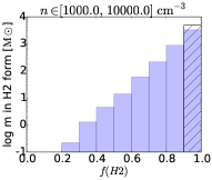
Figure 10: Mass in H₂ form per density bin. Comparison between the simulation (blue) and the calculation at equilibrium (dashed) for different timesteps. From left to right: $t=5,10,15,$ and $20\leavevmode\nobreak\ \mathrm{Myr}$. From top to bottom: density bins $n\leavevmode\nobreak\ \in\leavevmode\nobreak\ (0.1,1),(1,10),(10,100),(100,1000),(1000,10000)\leavevmode\nobreak\ \mathrm{[cm^{-3}]}$. Note the change of vertical scale.

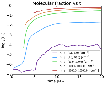
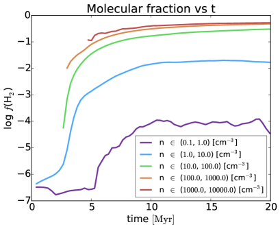
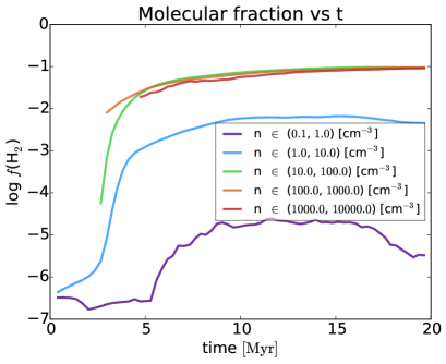
Figure 11: Evolution of the molecular fraction, where the formation of H₂ has been suppressed for gas denser than a fixed threshold. The top panel corresponds to the standard case, with no suppression of H₂ formation. The middle panel shows the evolution for a density threshold of $n=1000\leavevmode\nobreak\ \mathrm{[cm^{-3}]}$, while the panel at the bottom corresponds to a density threshold of $n=100\leavevmode\nobreak\ \mathrm{[cm^{-3}]}$

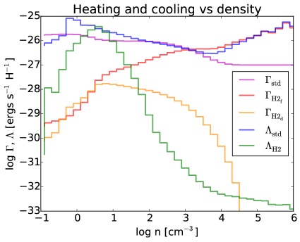
Figure 12: Various cooling and heating contributions as a function of density. As can be seen, H₂ does not have a dominant influence except at densities of about 4 cm^-3 where H₂ cooling (green line) becomes comparable to the standard ISM cooling (blue line) and at high densities where the heating by H₂ formation (red line) is significant (but without modifying the temperature substantially).

4 Results

We now present the results of our calculations. We start by discussing the general properties of the clouds because it is essential to understand in which context the hydrogen molecules form. Then we discuss the abundance and distribution of H₂ itself. Finally, we perform various complementary calculations aiming at better understanding in which conditions H₂ forms.

4.1 Qualitative description of the cloud

As many colliding flow calculations have been performed during the past decade, we do not attempt here to display all the steps that the flow experiences (see references above for accurate descriptions), so we quickly summarise the main steps. First, the WNM flows collide, which triggers the transition for a fraction of the gas into moderately dense gas , that is to say, densities of the order of 100-1000 cm^-3 as a consequence of the thermal instability and ram pressure. Second, when enough gas has been accumulated, gravity becomes important and triggers infall, first at small scales and then at larger ones. This leads to a continuous increase of the dense gas fraction.

The left panels of Figs. 1 and 2 show the column density along the $z$-direction and a density cut in the $xy$ plane at time 20 Myr, respectively. As we show below, this corresponds to a phase where gravity already plays a significant role. The density cut shows that the flow is very fragmented. The dense gas is organised into dense clumps that are embedded in diffuse and warm gas. The column density typically spans 2-3 orders of magnitude from a few 10²¹ cm^-2 to at least 10²⁴ cm^-2 in some very compact regions, the dense cores in which gravity triggers strong infall. The column density map is also clumpy, but less obviously structured than the density cut.

4.1.1 Density PDF and volume filling factor

In many respects the density distribution is an essential cloud property that reveals the dynamical state of the cloud and strongly influences the formation of H₂.

Figure 3 shows the density probability distribution function (PDF) at time 5, 10, 15, and 20 Myr. The peak at low density ($n\simeq 1$ cm^-3) is simply a consequence of the initial conditions and boundary conditions (which inject WNM from the boundaries), the rest, at higher densities, represents the cold phase, whose formation has been triggered by the thermal instability. Because of the supersonic turbulence that develops in the cold gas, the density PDF is broad and presents a lognormal shape (Kritsuk et al. 2007; Federrath et al. 2008). At later times, more cold gas accumulates and the PDF broadens. The high-density tail tends to become less steep. At intermediate densities ($\rho\sim$ 10³-10⁴ cm^-3) the shape is compatible with a power law with an exponent between -1 and -2. This is typical of what has been found in super-sonic turbulent simulations that include gravity (Kritsuk et al. 2011). At very high densities ($>10^{4}-10^{5}$ cm^-3), the density field flattens. This occurs because we did not use sink particles, and the very dense gas therefore piles up and accumulates within a few grid cells. This feature is thus a numerical artefact and represents a limit of the simulations.

Figure 4 shows the density PDF for different computational box regions at a time of 20 Myr. The four lines show the results for four different box regions (as shown in the label). The black line shows the whole box, the red line is limited to the densest regions of the computational box. The volume filling factor is clearly dominated by the warm and diffuse gas. Selecting gas of densities $n<3$ cm^-3, we find that it typically occupies 70$\%$ for the region located between $x=27$ and $x=37$ (85$\%$ for the whole computational box). The dense gas, even in the densest region, occupies only a tiny fraction, for example we find that the gas denser than 100 cm^-3 has a filling factor of about 3$\%$ (respectively 1.5$\%$ for the whole box). The remaining 26$\%$ (13$\%$) are filled with gas of densities between 3 and 100 cm^-3. We therefore conclude that the interclump medium that occupies most of the volume, is itself made of two components: a warm gas that is similar to the standard WNM, but can be slightly denser, and a cold gas that is similar to the CNM, but contains, as we show below, a significant fraction of H₂. They typically occupy about 70$\%$ and 25$\%$ percent of the volume, respectively.

4.1.2 Pressure of various phases

Another important diagnostic for characterizing the dynamics of a medium are the different pressures. Figure 5 shows the thermal, $P_{th}$, dynamical, $P_{ram}$, and magnetic, $P_{mag}$, pressures equal to $P_{th}=nkT$, $P_{ram}=\rho V^{2}$ and $P_{mag}=B^{2}/8\pi$, respectively.

The dynamical pressure clearly dominates the thermal pressure by typically one to two orders of magnitude in the dense gas ($n>10$ cm^-3), while they are more similar in the diffuse gas. The magnetic pressure lies in between the two, with values a few times higher than that of the thermal pressure. $P_{ram}$ and $P_{mag}$ increase with density, and at densities of the order of $n\simeq 10^{3}$ cm^-3, they are about one order of magnitude higher than their mean values at $n\simeq 10$ cm^-3. This means that while the low-density gas that fills the volume provides some confining pressure, it has a limited influence on the clumps.

Altogether, these results indicate that the molecular cloud produced in this calculation can be described by density fluctuations or clumps, induced by both ram pressure and gravity. The clumps occupy a tiny fraction of the volume, which is filled by a mixture of warm diffuse and dense HI gas (occupying a fraction ¿70$\%$ and ¿$20\%$ of the volume, respectively). This low-density material feeds the clumps, which grow in mass. This picture agrees well with the measurement performed by Williams et al. (1995), who found that the interclump medium typically has a density of a few particles per cm^-3 and a high velocity dispersion of several km s^-1.

4.1.3 Clump statistics

Because the cloud is organised into clumps, we further quantified the simulations by providing some statistics. To identify the clumps, we used a density threshold of 1000 cm^-3 and a friends-of-friends algorithm. This structure is important for the chemistry evolution because very significant density and temperature gradients arise at the edge of clumps . Figure 6 shows the mass spectrum, the velocity dispersion, and the kinetic $\beta$ parameter (that is to say, $P_{ram}/P_{mag}$) of the clumps. The mass spectrum for masses above a few 0.1 $M_{\odot}$ presents a power law with an index of about $-1.7$, which is very similar to what has been shown in related works (e.g. Audit & Hennebelle 2010; Heitsch et al. 2008b). The velocity dispersion within the clumps as a function of their size is about $\sigma\simeq 1\leavevmode\nobreak\ {\rm km\,s^{-1}}(L/1{\rm pc})$, which is close to the Larson relation (Larson 1981; Hennebelle & Falgarone 2012). The third panel shows that the kinetic $\beta$ parameter is typically of the order of, or slightly below 1, showing that the magnetic field plays an important role within the clumps.

4.2 Molecular hydrogen

We now discuss the H₂ abundance. The middle and right panels of Fig. 1 show the H₂ column density and molecular abundance, $f(\mathrm{H}_{2})=2n(\mathrm{H}_{2})/n$. As expected, the high column density regions are dominated by the H₂ molecules, and values of $f({\rm H}_{2})$ close to 1 are obtained there. The values of $f({\rm H}_{2})$ are obviously significantly lower in the outer parts of the cloud.

4.2.1 UV screening factor

The middle and right panels of Fig. 2 show a cut of $n({\rm H}_{2})$ and the value of the shielding parameter, $\chi_{\rm shield}=k_{\mathrm{ph}}/k_{\mathrm{ph,0}}$. This latter steeply decreases when entering the cloud, where it takes values of the order of $10^{-3}$. A comparison between the density cut with $k_{\mathrm{ph}}/k_{\mathrm{ph,0}}$ reveals that there are regions of diffuse material in which the shielding parameter is low. This is because these regions are surrounded by dense gas in which H₂ is abundant, which provides an efficient self-shielding. As a consequence, there are low-density regions that contain a relatively high abundance of H₂ (see left and middle panels of Fig. 2).

A more quantitative statement can be drawn from Fig. 7, which displays the distribution of the dust shielding, $\chi$ (top panel), and of the total shielding $\chi_{\rm shield}$ as a function of density (bottom panel). As expected, most low-density cells are associated with $\chi$ values that are close to 1, that is to say, they are weakly shielded. There is a fraction of them, however, that presents values of $\chi_{\rm shield}$ as low as 10^-5. At higher densities, the mean value of $\chi$ decreases with a steep drop between $n\simeq 10^{3}$ and $10^{4}$ cm^-3 , which corresponds to the point where the dust significantly absorbs the UV external field. For the total shielding, a steep drop is observed at about 10 cm^-3. There is a broad scatter, however, which increases from $n=1$ to $n=10^{4}$ cm^-3 for the dust shielding and tends to decrease for the total shielding $\chi_{\rm shield}$. This indicates that the mean value of $\chi_{\rm shield}$ is not sufficient information to quantify the abundance of H₂ expected at a given density. This is a clear consequence of the complex cloud structure. Since $\chi_{\rm shield}$ plays a key role in the formation of H₂, this complex distribution certainly makes molecular hydrogen formation in a multiphase turbulent cloud a complicated problem.

4.2.2 Global evolution of molecular hydrogen

Figure 8 shows $f({\rm H}_{2})$, the mean molecular fraction within the whole cloud, as a function of time. During the first 5 Myr, $f({\rm H}_{2})$ exponentially increases from nearly 0 to about $\simeq 0.1$. After this phase, $f({\rm H}_{2})$ continues to increase in a more steady almost linear way. Near 15 Myr, about 40$\%$ of the gas is in H₂ molecules. Since, as discussed before, the cloud is rather inhomogeneous in density and temperature, we also plot the time evolution per bin of density and temperature. The corresponding curves are displayed in Fig. 9. As expected, the total distribution closely follows the values of the densest bins, that is to say, it corresponds to densities higher than 100-1000 cm^-3. For these densities, the timescale for H₂ formation is thus of a few ($\simeq 6-8$) Myr. As recalled previously, this typical timescale is about $10^{9}/n$ yr. The timescale we observe in the simulation therefore agrees well with this scaling. Altogether, this agrees well with the results of Glover & Mac Low (2007a, b), who found that H₂ could be formed quickly in molecular clouds because it preferentially forms into clumps that are significantly denser than the rest of the cloud. In the present case, the mean density of our cloud at time 5-10 Myr would be about 10-100 cm^-3 (depending on exactly which area is selected), and this would lead to a timescale for H₂ formation of the order of 10 to 100 Myr.

The relatively short amount of time ($\simeq 10$ Myr) after which there is a significant amount of H₂ in low density gas ($n\simeq 1-10$ cm^-3) is somewhat more surprising. The expected timescale for H₂ formation in this density range would be about 10⁸ Myr. Figure 9 shows that the behaviour of $f({\rm H}_{2})$ is similar, although not identical, to the behaviour at higher densities. There is a fast increase followed by a slowly increasing phase. The slope changes at about 4 Myr however, and this is different from the higher density evolution. The steady evolution starts at about 8 Myr instead of 5-6 Myr for the denser regions. This suggests that the presence of H₂ at low density is triggered by formation of H₂ in the dense gas. This can occur in various non-exclusive ways. First of all, some dense gas can expand back and mix with diffuse gas. This may occur either through a sonic expansion, through evaporation, or through numerical diffusion. Second of all, some of the diffuse gas may be surrounded by dense gas in which $f({\rm H}_{2})$ is large and therefore has a low $\chi_{\rm shield}$. Below we attempt to analyse these mechanisms in more detail.

Finally, we note that in the bottom panel of Fig. 9 there is a small (1-10$\%$) but nevertheless non-negligible fraction of H₂ within gas of relatively high temperature, that is, $T>300$ K. Since H₂ is the first molecule involved in producing other molecules and since some of them, such as CH⁺, are formed through reactions with high activation barriers (of the order of $4300\leavevmode\nobreak\ \mathrm{K}$ for CH⁺, see Agúndez et al. 2010), the presence of H₂ could have consequences for the production of these species, as proposed in Lesaffre et al. (2007). In the same way, as discussed below, this warm H₂ contains molecules in excited high $J$ rotational levels, which can therefore contribute to the gas cooling.

4.2.3 Detailed distribution of molecular hydrogen

To further quantify the distribution of H₂ in the cloud, we display histograms of $f({\rm H}_{2})$ per density bin (Fig. 10). We also draw the distribution of $f({\rm H}_{2})$ obtained at equilibrium in the same panel. Knowing the density, $n$, the temperature, $T$ and the shielding factor, $\chi_{\rm shield}$, we solve Eq. (6) at equilibrium. We note that this distribution is not fully self-consistent since the value of $\chi_{\rm shield}$ should in principle be recalculated to be consistent with this equilibrium distribution (this would imply performing several iterations). In practice, the goal here is simply to compare with the time-dependent distribution to gain insight into the H₂ production mechanisms, and it is therefore easier to have exactly the same formation and destruction rates.

In particular, the equilibrium distribution is expected to be different from the time-dependent distribution for at least two main reasons. First, since the H₂ formation timescale is somewhat long, if the time-dependent $f({\rm H}_{2})$ lies below the equilibrium timescale, it will indicate that the H₂ abundance has been limited by the time to form the molecule. Second, if the time-dependent $f({\rm H}_{2})$ is above the equilibrium value, it will indicate that $f({\rm H}_{2})$ has increased because of an enrichment coming from denser gas. As discussed above, this could operate through the expansion or the evaporation of cold clumps, a process that we call turbulent diffusion, or through numerical diffusion. The latter is quantified in the appendix by performing convergence studies that suggest that it remains limited. Another possibility is that the H₂ excess has been produced during a phase where the fluid parcel was more shielded by the surrounding material and therefore the UV field was lower. The two effects probably act simultaneously and are difficult to separate.

At a time of 5 Myr (left panels), all density bins show an excess of the equilibrium distribution with respect to the time-dependent distribution. This is clearly due to the long timescale needed to form H₂. The differences between the equilibrium and time-dependent distributions become eventually less important. For example, the two distributions are obviously closer at a time of 20 Myr (right panels) than at a time of 5 Myr. However, they are not identical. Since all distributions at a time of 15 Myr and 20 Myr are similar, the persistence of the differences between the equilibrium and time-dependent distributions indicates that this is most likely the result of a stationary situation. It most likely reflects the accretion process, that is to say, HI gas (possibly mixed with a fraction of H₂) is continuously being accreted within denser clumps and therefore the dense gas does not become fully molecular. This interpretation is also consistent with the fact that the effect is more pronounced for the fourth density bin (line 4) than for the fifth and highest one (line 5). Considering now the lowest density bin (first line), we find the reverse effect at a time of 10 and 15 Myr: the time-dependent distribution dominates the equilibrium distribution. This is most likely an effect of the turbulent diffusion. Because of the low mass contained in this low-density bin, this remains a limited effect, however.

The second density bin (line 2), which corresponds to $n$ between 1 and 10 cm^-3 , is slightly puzzling. No significant differences are seen between the two distributions, which is surprising. One possibility is that various effects compensate for each other. That is to say, the time delay to form H₂ (clearly visible for the three denser density bins) may be compensated for by an enrichment from the denser gas. This might possibly occur for the second density bin at time 20 Myr (fourth column, second line) where overall a small excess of time-dependent H₂ is found, but for $f({\rm H}_{2})>0.7$ the equilibrium distribution dominates.

4.2.4 Spatial fluctuations

As a complement to the time evolution of $f({\rm H}_{2})$, it is also worthwhile to investigate the spatial fluctuations at a given time. In this respect, the clumps constitute natural entities for studying the spatial variations. The bottom panel of Fig. 6 shows $f({\rm H}_{2})$ within the clumps. For the most massive clumps, the value of $f({\rm H}_{2})$ is close to 1 and the dispersion remains weak. In contrast, the dispersion becomes very high for the less massive clumps, and the value of $f({\rm H}_{2})$ can in some circumstances be rather low. This shows that clump histories, that is to say, their ages and the local UV flux in which they grow, have a major influence on $f(\mathrm{H_{2}})$.

4.2.5 Further analysis of H₂ formation

To better quantify the interdependence of the different density bins, we conducted three complementary low-resolution runs for which the formation of H₂ was suppressed ($k_{\mathrm{form}}$ was set to zero) above a given density threshold. Figure 11 displays the result. In the top panel, no threshold is applied. In the middle and bottom panels a threshold of 1000 cm^-3 and 100 cm^-3, respectively, is applied. For the threshold 1000 cm^-3, the values of $f({\rm H}_{2})$ are not significantly changed except for the highest density range (for $n>1000$ cm^-3). On the other hand, with a threshold 100 cm^-3, the values of $f({\rm H}_{2})$ decrease by a factor of about 3 for all density bins. This clearly shows that most of the H₂ molecules in the low-density gas form at a density of a few 100 cm^-3. While the shielding provided by molecules in gas denser than this value could contribute to enhance the more diffuse gas, the filling factor of the dense gas is too small to strongly affect the diffuse gas, which has a much larger filling factor (see Fig. 4). Therefore we conclude that the H₂ abundance within the low-density gas (¡100 cm^-3) is very likely a consequence of turbulent mixing and gas exchange between diffuse and dense gas.

4.3 Thermal balance

To quantify the influence of the H₂ molecule on thermodynamics, we present the contributions of the various heating and cooling terms to the thermal balance as a function of density. Figure 12 shows the standard ISM cooling (blue curve) and the cooling by H₂ (green curve). The latter clearly remains below the former throughout, except at a density of about 3-5 cm^-3 , where they become similar. At densities above $3\times 10^{4}\leavevmode\nobreak\ \mathrm{cm^{-3}}$ the ”standard” heating curve (magenta) is dominated by the heating caused by cosmic rays and reaches the intermediate value for shielded gas proposed by Goldsmith (2001). While the heating due to H₂ destruction remains negligible at any density (orange curve), the heating due to its formation (red curve) is the dominant heating mechanism at high densities. This does not affect the temperature very strongly, however. It remains equal to about 10 K. Moreover, at higher densities (above $\sim 10^{5}\leavevmode\nobreak\ \mathrm{cm^{-3}}$ ) other processes that are not included in our simulations can take over, such as collisions with dust grains and the cooling by other molecular lines, such as CO.

Finally, as can be seen for densities between $1$ to $\sim 50\leavevmode\nobreak\ \mathrm{cm^{-3}}$, the cooling dominates the heating by a factor of a few. This indicates that there is another source of heating equal to the difference, which is due to the mechanical energy dissipation. This latter therefore appears to have a contribution similar to the UV heating. This explains why warm gas is actually able to survive within molecular clouds. In the same way that density is much higher than in the rest of the ISM, kinetic energy is also higher and provides a significant heating (e.g. Hennebelle & Inutsuka 2006).

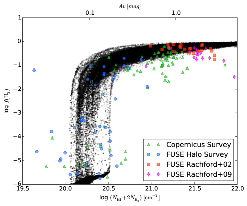
Figure 13: Molecular fraction as a function of total hydrogen column density. Comparison with the Copernicus survey (Savage et al. 1977) and FUSE (Gillmon et al. 2006; Rachford et al. 2002, 2009).

5 Comparison to observations

We now compare our results with various observations that fall into two categories. The first observations have attempted to measure the molecular fraction, that is, the total column density of H₂ with respect to the total column density. The second observations have measured the excited levels of H₂, therefore presumably tracing high-temperature gas. These two sets of observations are therefore complementary and very informative.

5.1 Molecular fraction vs column density

The H₂ column density has been estimated along several lines of sight mainly (though not exclusively) with the Copernicus satellite (Savage et al. 1977) and the FUSE observatory (Gillmon et al. 2006; Rachford et al. 2002, 2009). These observations probe lines of sight spanning a wide range of column densities and therefore constitute a good test for our simulations, although a difference to keep in mind is that the lines of sight extracted from our simulations are all taken from a $50\leavevmode\nobreak\ \mathrm{pc}$ region and therefore are more homogeneous than the observed lines of sight.

Figure 13 shows the molecular fraction $f({\rm H}_{2})$ as a function of total column density for all lines of sight of the simulations (taken along the $z$-direction) and the available lines of sight reported in Gillmon et al. (2006), and Rachford et al. (2002, 2009). The simulation results and the observations agree rather well, many observational data directly fall into the same regions as simulated data. In particular, the two regimes, that is, the vertical transition branch at column densities of between $10^{20}$ and $3\times 10^{20}\leavevmode\nobreak\ \mathrm{cm}^{-3}$ as well as the higher column density region, are clearly seen both in observations and in the simulation.

This said, there are also data points that are not reproduced by any of the lines of sight from the simulations. This is particularly the case for column densities higher than $3\times 10^{21}\leavevmode\nobreak\ \mathrm{cm}^{-2}$ and for the Copernicus survey at column densities of around $\simeq 10^{21}\leavevmode\nobreak\ \mathrm{cm}^{-2}$. The most likely explanation is that the UV flux is different from the standard value we assumed in our study. We stress in particular that the measurements were made in absorption toward massive stars. Because these are strong emitters of UV radiation, it may not be too surprising that our measurements lead to higher values of $f({\rm H}_{2})$. A more quantitative estimate should entail a detailed modelling of every line of sight, including the UV flux in the regions of interest and specific cloud parameters, such as column densities. This is beyond the scope of the present paper.

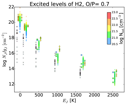
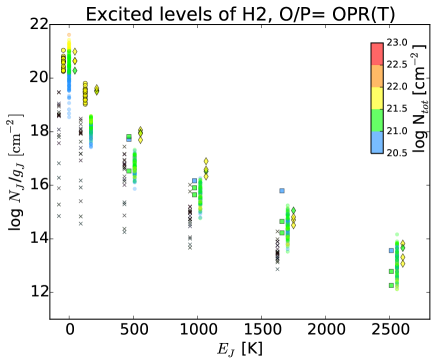
Figure 14: H₂ population distribution along different lines of sight at a time $t=20\leavevmode\nobreak\ \mathrm{Myr}$, using an ortho-to-para ratio of $0.7$ (top), and at thermal equilibrium (bottom). The symbols correspond to the observational data of Wakker (2006) (cross), Rachford et al. (2002) (circle), Gry et al. (2002) (square), and Lacour et al. (2005) (diamond). Colours correspond to the total column density range.

Figure 15: H₂ level population distribution for individual cells in the simulation calculated at $20\leavevmode\nobreak\ \mathrm{Myr}$: using an ortho-to-para ratio OPR = $0.7$ (top) and at thermal equilibrium (bottom).

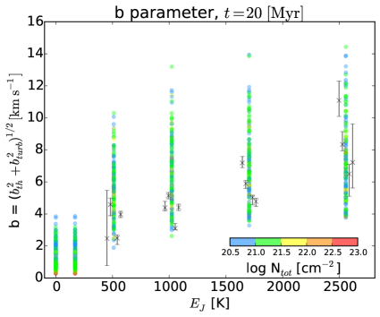
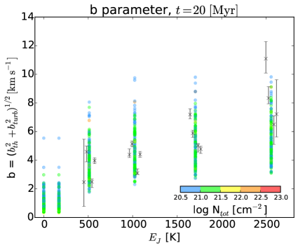
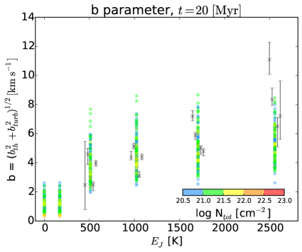
Figure 16: $b$-parameter along several lines of sight for excited levels of H₂ and comparison with the data from Lacour et al. (2005). The top panel shows lines of sight along the $x$-axis, the middle panel those along the $y$-axis, and the bottom panel the lines along the $z$-axis.

5.2 Excited levels of H₂

We now compare our results with the observations of rotational levels of the H₂ molecule, which require high temperatures to be excited.

As investigated by previous authors (Lacour et al. 2005; Godard et al. 2009), these data cannot be explained by pure UV excitation. While Lacour et al. (2005) concluded that to explain the observations, a warm layer associated with the cold gas should be present, Godard et al. (2009) performed detailed modelling that entailed shocks or vortices. The general idea is that in such dissipative small -scale structures the temperature reaches high values because of the intense mechanical heating. Interestingly, Godard et al. (2009) obtained a nice agreement between their model and the data. We stress that the small dissipative scales that are determinant in these models cannot be described in our simulations, which have a limited resolution of the order of $\simeq 0.1\leavevmode\nobreak\ \mathrm{pc}$. On the other hand, as our simulations contained large quantities of warm H₂, it is worthwhile to investigate whether the inferred populations of excited H₂ can be reproduced quantitatively.

5.2.1 Calculation of population levels and column densities

We calculated the population of the first six rotational levels ($J$) of $\mathrm{H_{2}}$ as in Flower et al. (1986), based on the approach of Elitzur & Watson (1978). This calculation was made in post-processing for all grid cells. It needs the total hydrogen number density, the $\mathrm{H_{2}}$ number density, the $\mathrm{He}$ number density (we assumed $10\%$ of the total $\mathrm{H}$), the temperature, and the ortho-to-para ratio (OPR). It assumes thermal equilibrium and includes spontaneous de-excitation and collisional excitation by $\mathrm{HI}$, by $\mathrm{He}$, and by other $\mathrm{H_{2}}$ molecules.

The OPR is not very well known in the ISM (e.g. Le Bourlot 2000) and may need a specific time-dependent treatment, which is beyond the scope of this paper. Even though the OPR of newly formed H₂ molecules is thought to take values close to 3 (Takahashi 2001), observations differ. In high-density regions ($n(\mathrm{H_{2}})\sim 10^{5}\leavevmode\nobreak\ \mathrm{cm}^{-3}$) observations seem to favour values as low as $0.25$ (Neufeld et al. 2006; Pagani et al. 2011; Dislaire et al. 2012), while in translucent clouds intermediate values close to $0.7$ are preferred (Myers et al. 2015; Gry et al. 2002; Lacour et al. 2005; Nehmé et al. 2008; Ingalls et al. 2011; Rachford et al. 2009). Because we investigate the role of low-density gas regions in the distribution of excited rotational levels of H₂, we assumed an OPR= $0.7$, suitable for translucent clouds such as those produced in our simulations. We also considered for comparison an OPR given by thermal equilibrium that reaches the statistical weight of 3 at high temperatures ($T\gtrsim 300\leavevmode\nobreak\ \mathrm{K}$).

After we obtained the populations of the H₂ rotational levels and column density, we integrated along several lines of sight in the $z$-direction.

5.2.2 Comparison with observed column densities

Figure 14 shows the distribution of the column densities corresponding to the various rotational levels in the simulation. The top panel shows results for an OPR equal to $0.7,$ while the bottom panel shows results for the thermal equilibrium assumption. The colour coding shows the total column density of the corresponding line of sight. The symbols correspond to the observational data of Wakker (2006) (cross), Rachford et al. (2002) (circle), Gry et al. (2002) (square), and Lacour et al. (2005) (diamond).

The simulation results are divided into two groups of points, very low column densities coming from the WNM that is located outside the molecular cloud (blue points) and higher column densities (green and yellow points) that come from the gas belonging to the molecular cloud. For the $J=0$ and 1 levels, the column densities are more or less proportional to the total column density. This is indeed expected since most of H₂ molecules are in one of these two levels. Their respective abundance significantly depends on the assumption used for the OPR. While there is about a factor 10 between the first two rotational levels for $N_{J}/g_{J}$ when the OPR is equal to 0.7, it is almost a factor thousand when the OPR is assumed to be at thermal equilibrium.

The situation is different for the higher levels. The highest column densities of the excited rotational levels do not correspond to the highest total hydrogen column densities, and there is generally no obvious correlation between the two. This is because the high $J$ levels come from the warm gas (with temperatures of between a few hundred and a few thousand Kelvin), which itself has a low column density and is largely independent of the cold gas.

The comparison with the observational data is very enlightening. The agreement with the simulation results is very good in general. The observational data points have column densities that are very similar to the simulation data. The best agreement is found for OPR$=0.7$ , for which the simulation data points are slightly above the observational ones, while for an OPR at thermal equilibrium simulation data points are below the observed points. This probably suggests that the actual OPR lies in between, close to $0.7$. This might be in conflict with some of the data of Gry et al. (2002) and Lacour et al. (2005) for $J=2$ by about a factor on the order of 3-10. If confirmed, this would indicate that another mechanism, such as the one proposed by Godard et al. (2009), could operate and contribute to excite H₂.

To help understand the origin of the excited rotational levels in the simulation, Fig. 15 displays the mean density of the H₂ excited levels for five density bins and the complete distribution for the two OPR used in this work. Figure 15 shows that the choice of the OPR mainly affects the dense, and thus colder gas, which is the main contributor to the populations of the two first levels ($J=0$ and $J=1$). The OPR at thermal equilibrium for very dense and cold gas is close to zero, which dramatically affects the ratio between the populations of these two levels. At lower densities in warmer gas, the OPR becomes closer to $3$, but the populations do not differ much from those calculated using OPR= $0.7$. For the excited level the highest contributions are found in gas of total density between 1 and 10 cm^-3. This means that very diffuse gas with $n<1$ cm^-3 and moderately dense gas (with $n$ between 10 and 100 cm^-3) contribute in roughly equal proportions to the excited levels. We recall that the peak of the cooling contribution of H₂ lies precisely in this density domain (see Fig. 12).

5.2.3 Velocity dispersion of individual rotational levels

The conclusion we can draw so far is that the population of the excited levels of H₂ ($J\geq 2$) is dominated by the warm H₂ that is interspersed between the cold and dense molecular clumps. This ”layer” of warm gas is directly associated with the molecular cloud and agrees well with the proposition made by Lacour et al. (2005). These authors made another interesting observation. They found that the width of the lines associated with the excited levels increases with $J$. To investigate whether our simulation exhibits the same trends, we calculated the mean velocity dispersion along several (125 along each axis) lines of sight for each excited level. Figure 16 shows the mean Doppler-broadening parameter, $b$, linked to the velocity dispersion $\sigma$ by $b^{2}=2^{1/2}\sigma^{2}$, and where

$$\sigma^{2}={\int\rho\left((v_{i}-\langle v_{i}\rangle)^{2}+C_{s}^{2}\right)dx\over\int\rho dx},$$ (16)

where $C_{s}$ is the local sound speed, $v_{i}$ is the $i$ component of the local velocity, and $\langle v_{i}\rangle$ is the mean velocity along the $i$-direction. Figure 16 displays the results. Since the colliding flow configuration is highly non-isotropic, we calculated these velocity dispersions along the $x$-axis (top panel), the $y$-axis (middle panel), and the $z$-axis (bottom panel). While a more accurate treatment would consist of simulating the line profiles and then applying the same algorithm as the authors used, this simple estimate is already illustrative. From $\sigma^{2}$, we can infer the width of the line and the $b$ parameter.

The trends in the simulation and in the observations are similar. Higher $J$ levels tends to be associated with larger $b$. The agreement is quantiatively satisfying for the $y-$ and $z$-directions. Similar to the observations, the simulated lines of sight present a slightly higher velocity dispersion for higher $J$. The agreement is poor for the lines of sight along the $x$-direction because they present a dispersion that is too high with respect to the observations. This is most likely an artefact of the colliding flow configuration.

The trend of larger $b$ for higher $J$ stems for the fact that higher levels need warmer gas to be excited. Therefore the fluid elements, which are enriched in high rotational levels, have higher temperatures and therefore higher velocity dispersions (since both are usually correlated).

Altogether, these results suggest that the excited rotational level abundances reveal the complex structure of molecular clouds that is two-phase in nature and entails warm gas deeply interspersed with the cold gas due to the mixing induced by turbulence.

6 Conclusions

We have performed high-resolution magneto-hydrodynamical simulations to describe the formation of molecular clouds out of diffuse atomic hydrogen streams. We particularly focused on the formation of the H₂ molecule itself using a tree-based approach to evaluate UV shielding (see Valdivia & Hennebelle 2014).

In accordance with previous works (Glover & Mac Low 2007a), we found that H₂ is able to form much faster than simple estimates, based on cloud mean density, would predict. The reason for this is that because the clouds are supersonic and have a two-phase structure, H₂ is produced in clumps that are much denser than the clouds on average.

As a result of a combination of phase exchanges and high UV screening deep inside the multiphase molecular clouds (numerical convergence tests suggest that numerical diffusion is not responsible of this process), a significant fraction of H₂ develops even in the low-density and warm interclump medium. This warm H₂ contributes to the thermal balance of the gas, and in the range of density $3-10\leavevmode\nobreak\ \mathrm{cm}^{-3}$ its cooling rate is similar to the standard cooling rate of the ISM.

Detailed comparisons with Copernicus and FUSE observations showed a good agreement overall. In particular, the fraction of H₂ varies with the total gas column density in a very similar way, showing a steep increase between column densities $10^{20}$ and $3\times 10^{20}\leavevmode\nobreak\ \mathrm{cm}^{-3}$ and a slow increase at higher column densities. There is a trend for the high column density regions to present H₂ fractions significantly below the values inferred from the simulations, however. This is a possible consequence of the constant UV flux assumed in this work. Interestingly, the column densities of the excited rotational levels obtained at thermal equilibrium reproduce the observations fairly well. This is a direct consequence of the presence of H₂ molecules in the warm interclump medium and suggests that the H₂ populations in excited levels reveal the two-phase structure of molecular clouds.

Appendix A Numerical convergence: resolution study

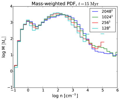
Figure 17: Mass-weighted density PDF for a series of numerical resolutions. The discrepancy between low- and high-resolution runs is very significant. The difference between the resolution of the standard and high resolution runs is low, except for the highest density bins, which contain little mass.

$t=10\leavevmode\nobreak\ \mathrm{Myr}$	$t=15\leavevmode\nobreak\ \mathrm{Myr}$

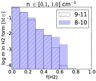
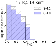
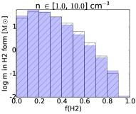
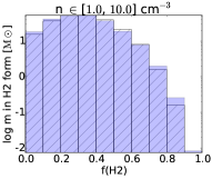
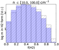
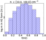
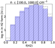
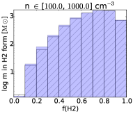
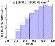
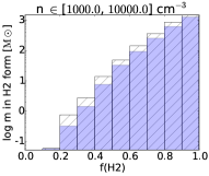
Figure 18: Mass in H₂ per density bin. Comparison between the standard resolution simulations (levels 8-10, in blue) and the high-resolution simulations (levels 9-11, dashed) at a time of $10$ and $15\leavevmode\nobreak\ \mathrm{Myr}$. From top to bottom: density bins $n\leavevmode\nobreak\ \in\leavevmode\nobreak\ (0.1,1),\ (1,10),\ (10,100),\ (100,1000),\ (1000,10000)\leavevmode\nobreak\ \mathrm{[cm^{-3}]}$. The differences between the two remain fairly limited, showing that numerical convergence is not a great problem.

Numerical resolution is a crucial issue particularly in the context of chemistry. Here we compare runs of various resolutions.

Figure 17 shows the mass-weighted density PDF at a time of $15\leavevmode\nobreak\ \mathrm{Myr}$ for four different resolutions, $128^{3}$, $256^{3}$, $1024^{3}$ , and $2048^{3}$ (for the two last and higher resolutions this represents the highest effective resolution since AMR was used, as described above). The density PDF of low-resolution runs is quite different from the higher ones, which shows the importance of the numerical resolution. The two highest resolution runs present similar but not identical PDFs. This suggests that for the highest resolution runs, numerical convergence for the density PDF is nearly reached, although strictly speaking, it would be necessary to perform runs with an even higher resolution. This conclusion agrees well with the results of Federrath (2013), who found that the density PDF converges for a resolution inbetween $1024^{3}$ and $2048^{3}$ for isothermal self-gravitating simulations.

Figure 18 shows $f({\rm H}_{2})$ distribution in five density bins at times of $10$ and $15\leavevmode\nobreak\ \mathrm{Myr}$ for the standard and high-resolution runs (effective $1024^{3}$ and $2048^{3}$ resolution). Overall, the two simulations agree well. The differences are similar to the differences found in the density PDF. In particular, this suggests that numerical diffusion is not primarily responsible of the fraction of warm H₂ that we observe at low density (as discussed in Sect. 4.2).

Appendix B Influence of the $b$ Doppler parameter

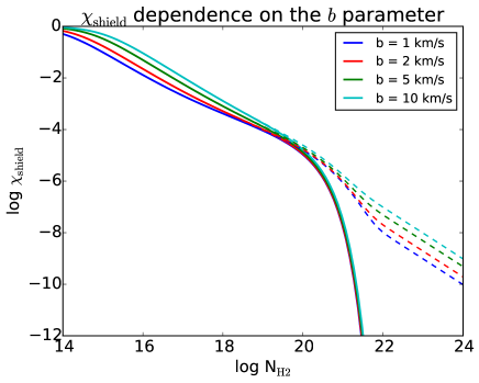
Figure 19: Total shielding coefficient for H₂, $\chi_{\mathrm{shield}}$, as a function of total H₂ column density for several values of the $b$ Doppler parameter. The dashed lines show the expected value in absence of shielding by dust.

Figure 19 shows the dependence of the total shielding coefficient for H₂ (shielding by H₂ and by dust) on the $b$ Doppler parameter as a function of total H₂ column density. The total column density was approximated as $\mathcal{N}_{\mathrm{tot}}\approx 2\times\mathcal{N}_{\mathrm{H_{2}}}$, which sets a lower limit to the influence of dust shielding. The $\chi_{\mathrm{shield}}$ parameter varies within less than one order of magnitude for different $b$ parameters ranging from $1$ to $10\leavevmode\nobreak\ \mathrm{km\ s^{-1}}$. In the H₂ column density range of interest ($\mathcal{N}_{\mathrm{H_{2}}}\sim 10^{17}-10^{22}\leavevmode\nobreak\ \mathrm{cm^{-2}}$) all values are very similar. At higher column densities the shielding is dominated by dust.

References

- Agúndez et al. (2010) Agúndez, M., Goicoechea, J. R., Cernicharo, J., Faure, A., & Roueff, E. 2010, ApJ, 713, 662
- Audit & Hennebelle (2005) Audit, E. & Hennebelle, P. 2005, A&A, 433, 1
- Audit & Hennebelle (2010) Audit, E. & Hennebelle, P. 2010, A&A, 511, A76
- Bakes & Tielens (1994) Bakes, E. L. O. & Tielens, A. G. G. M. 1994, ApJ, 427, 822
- Ballesteros-Paredes et al. (1999) Ballesteros-Paredes, J., Vázquez-Semadeni, E., & Scalo, J. 1999, ApJ, 515, 286
- Banerjee et al. (2009) Banerjee, R., Vázquez-Semadeni, E., Hennebelle, P., & Klessen, R. S. 2009, MNRAS, 398, 1082
- Bigiel et al. (2008) Bigiel, F., Leroy, A., Walter, F., et al. 2008, AJ, 136, 2846
- Black & Dalgarno (1977) Black, J. H. & Dalgarno, A. 1977, ApJS, 34, 405
- Blitz & Shu (1980) Blitz, L. & Shu, F. H. 1980, ApJ, 238, 148
- Bron et al. (2014) Bron, E., Le Bourlot, J., & Le Petit, F. 2014, A&A, 569, A100
- Burton et al. (1992) Burton, M. G., Hollenbach, D. J., & Tielens, A. G. G. 1992, ApJ, 399, 563
- Clark et al. (2012) Clark, P. C., Glover, S. C. O., Klessen, R. S., & Bonnell, I. A. 2012, MNRAS, 424, 2599
- Dislaire et al. (2012) Dislaire, V., Hily-Blant, P., Faure, A., et al. 2012, A&A, 537, A20
- Dobbs et al. (2014) Dobbs, C. L., Krumholz, M. R., Ballesteros-Paredes, J., et al. 2014, Protostars and Planets VI, 3
- Draine & Bertoldi (1996) Draine, B. T. & Bertoldi, F. 1996, ApJ, 468, 269
- Elitzur & Watson (1978) Elitzur, M. & Watson, W. D. 1978, A&A, 70, 443
- Federrath (2013) Federrath, C. 2013, MNRAS, 436, 1245
- Federrath et al. (2008) Federrath, C., Klessen, R. S., & Schmidt, W. 2008, ApJ, 688, L79
- Flower et al. (1986) Flower, D. R., Pineau-Des-Forets, G., & Hartquist, T. W. 1986, MNRAS, 218, 729
- Fromang et al. (2006) Fromang, S., Hennebelle, P., & Teyssier, R. 2006, A&A, 457, 371
- Gillmon et al. (2006) Gillmon, K., Shull, J. M., Tumlinson, J., & Danforth, C. 2006, ApJ, 636, 891
- Glover & Clark (2014) Glover, S. C. O. & Clark, P. C. 2014, MNRAS, 437, 9
- Glover & Mac Low (2007a) Glover, S. C. O. & Mac Low, M.-M. 2007a, ApJS, 169, 239
- Glover & Mac Low (2007b) Glover, S. C. O. & Mac Low, M.-M. 2007b, ApJ, 659, 1317
- Gnedin & Kravtsov (2011) Gnedin, N. Y. & Kravtsov, A. V. 2011, ApJ, 728, 88
- Godard et al. (2009) Godard, B., Falgarone, E., & Pineau Des Forêts, G. 2009, A&A, 495, 847
- Goldsmith (2001) Goldsmith, P. F. 2001, ApJ, 557, 736
- Gould & Salpeter (1963) Gould, R. J. & Salpeter, E. E. 1963, ApJ, 138, 393
- Gry et al. (2002) Gry, C., Boulanger, F., Nehmé, C., et al. 2002, A&A, 391, 675
- Habart et al. (2011) Habart, E., Abergel, A., Boulanger, F., et al. 2011, A&A, 527, A122
- Habing (1968) Habing, H. J. 1968, Bull. Astron. Inst. Netherlands, 19, 421
- Hayes & Nussbaumer (1984) Hayes, M. A. & Nussbaumer, H. 1984, A&A, 134, 193
- Heitsch et al. (2005) Heitsch, F., Burkert, A., Hartmann, L. W., Slyz, A. D., & Devriendt, J. E. G. 2005, ApJ, 633, L113
- Heitsch et al. (2008a) Heitsch, F., Hartmann, L. W., & Burkert, A. 2008a, ApJ, 683, 786
- Heitsch et al. (2008b) Heitsch, F., Hartmann, L. W., Slyz, A. D., Devriendt, J. E. G., & Burkert, A. 2008b, ApJ, 674, 316
- Heitsch et al. (2006) Heitsch, F., Slyz, A. D., Devriendt, J. E. G., Hartmann, L. W., & Burkert, A. 2006, ApJ, 648, 1052
- Hennebelle et al. (2008) Hennebelle, P., Banerjee, R., Vázquez-Semadeni, E., Klessen, R. S., & Audit, E. 2008, A&A, 486, L43
- Hennebelle & Falgarone (2012) Hennebelle, P. & Falgarone, E. 2012, A&A Rev., 20, 55
- Hennebelle & Inutsuka (2006) Hennebelle, P. & Inutsuka, S.-i. 2006, ApJ, 647, 404
- Hennebelle & Pérault (1999) Hennebelle, P. & Pérault, M. 1999, A&A, 351, 309
- Hennebelle & Pérault (2000) Hennebelle, P. & Pérault, M. 2000, A&A, 359, 1124
- Hollenbach & Salpeter (1971) Hollenbach, D. & Salpeter, E. E. 1971, ApJ, 163, 155
- Hollenbach et al. (1971) Hollenbach, D. J., Werner, M. W., & Salpeter, E. E. 1971, ApJ, 163, 165
- Ingalls et al. (2011) Ingalls, J. G., Bania, T. M., Boulanger, F., et al. 2011, ApJ, 743, 174
- Inoue & Inutsuka (2012) Inoue, T. & Inutsuka, S.-i. 2012, ApJ, 759, 35
- Jura (1974) Jura, M. 1974, ApJ, 191, 375
- Kennicutt & Evans (2012) Kennicutt, R. C. & Evans, N. J. 2012, ARA&A, 50, 531
- Körtgen & Banerjee (2015) Körtgen, B. & Banerjee, R. 2015, ArXiv e-prints
- Koyama & Inutsuka (2002) Koyama, H. & Inutsuka, S.-i. 2002, ApJ, 564, L97
- Kritsuk et al. (2007) Kritsuk, A. G., Norman, M. L., Padoan, P., & Wagner, R. 2007, ApJ, 665, 416
- Kritsuk et al. (2011) Kritsuk, A. G., Norman, M. L., & Wagner, R. 2011, ApJ, 727, L20
- Krumholz et al. (2008) Krumholz, M. R., McKee, C. F., & Tumlinson, J. 2008, ApJ, 689, 865
- Lacour et al. (2005) Lacour, S., Ziskin, V., Hébrard, G., et al. 2005, ApJ, 627, 251
- Lada et al. (2012) Lada, C. J., Forbrich, J., Lombardi, M., & Alves, J. F. 2012, ApJ, 745, 190
- Larson (1981) Larson, R. B. 1981, MNRAS, 194, 809
- Launay & Roueff (1977) Launay, J.-M. & Roueff, E. 1977, Journal of Physics B Atomic Molecular Physics, 10, 879
- Le Bourlot (2000) Le Bourlot, J. 2000, A&A, 360, 656
- Le Bourlot et al. (2012) Le Bourlot, J., Le Petit, F., Pinto, C., Roueff, E., & Roy, F. 2012, A&A, 541, A76
- Le Bourlot et al. (1999) Le Bourlot, J., Pineau des Forêts, G., & Flower, D. R. 1999, MNRAS, 305, 802
- Leroy et al. (2013) Leroy, A. K., Walter, F., Sandstrom, K., et al. 2013, AJ, 146, 19
- Lesaffre et al. (2007) Lesaffre, P., Gerin, M., & Hennebelle, P. 2007, A&A, 469, 949
- Levrier et al. (2012) Levrier, F., Le Petit, F., Hennebelle, P., et al. 2012, A&A, 544, A22
- Micic et al. (2013) Micic, M., Glover, S. C. O., Banerjee, R., & Klessen, R. S. 2013, MNRAS, 432, 626
- Micic et al. (2012) Micic, M., Glover, S. C. O., Federrath, C., & Klessen, R. S. 2012, MNRAS, 421, 2531
- Moos et al. (2000) Moos, H. W., Cash, W. C., Cowie, L. L., et al. 2000, ApJ, 538, L1
- Myers et al. (2015) Myers, A. T., McKee, C. F., & Li, P. S. 2015, MNRAS, 453, 2747
- Nehmé et al. (2008) Nehmé, C., Le Bourlot, J., Boulanger, F., Pineau Des Forêts, G., & Gry, C. 2008, A&A, 483, 485
- Neufeld et al. (2006) Neufeld, D. A., Melnick, G. J., Sonnentrucker, P., et al. 2006, ApJ, 649, 816
- Pagani et al. (2011) Pagani, L., Roueff, E., & Lesaffre, P. 2011, ApJ, 739, L35
- Rachford et al. (2009) Rachford, B. L., Snow, T. P., Destree, J. D., et al. 2009, ApJS, 180, 125
- Rachford et al. (2002) Rachford, B. L., Snow, T. P., Tumlinson, J., et al. 2002, ApJ, 577, 221
- Santangelo et al. (2014) Santangelo, G., Antoniucci, S., Nisini, B., et al. 2014, A&A, 569, L8
- Savage et al. (1977) Savage, B. D., Bohlin, R. C., Drake, J. F., & Budich, W. 1977, ApJ, 216, 291
- Sheffer et al. (2008) Sheffer, Y., Rogers, M., Federman, S. R., et al. 2008, ApJ, 687, 1075
- Shull et al. (2000) Shull, J. M., Tumlinson, J., Jenkins, E. B., et al. 2000, ApJ, 538, L73
- Spitzer (1978) Spitzer, L. 1978, Physical processes in the interstellar medium
- Spitzer & Jenkins (1975) Spitzer, Jr., L. & Jenkins, E. B. 1975, ARA&A, 13, 133
- Sternberg et al. (2014) Sternberg, A., Le Petit, F., Roueff, E., & Le Bourlot, J. 2014, ApJ, 790, 10
- Takahashi (2001) Takahashi, J. 2001, ApJ, 561, 254
- Teyssier (2002) Teyssier, R. 2002, A&A, 385, 337
- Tielens (2005) Tielens, A. G. G. M. 2005, The Physics and Chemistry of the Interstellar Medium
- Valdivia & Hennebelle (2014) Valdivia, V. & Hennebelle, P. 2014, A&A, 571, A46
- Valentijn & van der Werf (1999) Valentijn, E. A. & van der Werf, P. P. 1999, ApJ, 522, L29
- Vázquez-Semadeni et al. (2010) Vázquez-Semadeni, E., Colín, P., Gómez, G. C., Ballesteros-Paredes, J., & Watson, A. W. 2010, ApJ, 715, 1302
- Vázquez-Semadeni et al. (2007) Vázquez-Semadeni, E., Gómez, G. C., Jappsen, A. K., et al. 2007, ApJ, 657, 870
- Vázquez-Semadeni et al. (2006) Vázquez-Semadeni, E., Ryu, D., Passot, T., González, R. F., & Gazol, A. 2006, ApJ, 643, 245
- Verstraete et al. (1999) Verstraete, L., Falgarone, E., Pineau des Forets, G., Flower, D., & Puget, J. L. 1999, in ESA Special Publication, Vol. 427, The Universe as Seen by ISO, ed. P. Cox & M. Kessler, 779
- Wakker (2006) Wakker, B. P. 2006, ApJS, 163, 282
- Williams et al. (1995) Williams, J. P., Blitz, L., & Stark, A. A. 1995, ApJ, 451, 252
- Wolfire et al. (1995) Wolfire, M. G., Hollenbach, D., McKee, C. F., Tielens, A. G. G. M., & Bakes, E. L. O. 1995, ApJ, 443, 152
- Wolfire et al. (2003) Wolfire, M. G., McKee, C. F., Hollenbach, D., & Tielens, A. G. G. M. 2003, ApJ, 587, 278
- Wong & Blitz (2002) Wong, T. & Blitz, L. 2002, ApJ, 569, 157