Effect of geometry and Reynolds number on the turbulent separated flow behind a bulge in a channel

Abstract

Turbulent flow separation induced by a protuberance on one of the walls of an otherwise planar channel is investigated using Direct Numerical Simulations. Different bulge geometries and Reynolds numbers – with the highest friction Reynolds number simulation reaching a peak of $\Rey_{\tau}=900$ – are addressed to understand the effect of the wall curvature and of the Reynolds number on the dynamics of the recirculating bubble behind the bump. Global quantities reveal that most of the drag is due to the form contribution, whilst the friction contribution does not change appreciably with respect to an equivalent planar channel flow. The size and position of the separation bubble strongly depends on the bump shape and the Reynolds number. The most bluff geometry has a larger recirculation region, whilst the Reynolds number increase results in a smaller recirculation bubble and a shear layer more attached to the bump. The position of the reattachment point only depends on the Reynolds number in agreement with experimental data available in the literature. Both the mean and the turbulent kinetic energy equations are addressed in such non homogeneous conditions revealing a non trivial behaviour of the energy fluxes. The energy introduced by the pressure drop follows two routes: part of it is transferred towards the walls to be dissipated and part feeds the turbulent production hence the velocity fluctuations in the separating shear layer. Spatial energy fluxes transfer the kinetic energy into the recirculation bubble and downstream near the wall where it is ultimately dissipated. Consistently, anisotropy concentrates at small scales near the walls irrespective of the value of the Reynolds number. In the bulk flow and in the recirculation bubble, isotropy is restored at small scales and the isotropy recovery rate is controlled by the Reynolds number. Anisotropy invariant maps are presented, showing the difficulty in developing suitable turbulence models to predict separated turbulent flow dynamics. Results shed light on the processes of production, transfer and dissipation of energy in this relatively complex turbulent flow where non-homogeneous effects overwhelm the classical picture of wall bounded turbulent flows which typically exploits streamwise homogeneity.

1 Introduction

Flow separation consists of fluid flow around bodies becoming detached, causing the fluid closest to the object’s surface to flow in reverse or different directions, most often giving rise to turbulent fluctuations. The flow separation can be induced either by geometrical singularities, for example in presence of sharp corners, or by smooth geometry variations, as those occurring over a curved wall. The resulting adverse pressure gradient is sufficient to cause flow detachment.

Given its importance from both theoretical and practical point of view, the study of turbulence and separation has long been of interest to the fluid mechanics community, see e.g. Simpson (1989) for a review. However, due to its complexity, this classic subject is still widely investigated. The separation of fluid flow from objects inevitably results in effects such as increased drag and mixing, momentum and energy transfer and vortex shedding. An understanding of such effects is helpful to improve road vehicle performance, in the study of fluid-structure interaction, to regulate air mixing with other substances such as pollutants or fuels, in the study of boundary layer control, see e.g. Marusic et al. (2014) and Bai et al. (2014). In modern bioengineering studies such as in hemodynamics, the nature of the flow and the intensity of the shear stresses helps to determine whether lesions occur at particular vascular sites, as described by Epstein & Ross (1999).

Turbulent boundary layers with pressure gradients are a common characteristic of many aerodynamic flows such as the flow past airfoils, gas turbine blades, sails and diffusers. To correctly predict the behaviour and the efficiency of such components, the understanding of separation and reattachment mechanisms together with the associated energy behaviour is essential, see e.g. Harun et al. (2013) and references therein. The fundamental physics is indeed complex and no entirely satisfactory turbulence models for numerical simulation of high Reynolds number separated flows are nowadays available. This is mainly due to the complexity of the geometries inducing separation and to the difficulty in obtaining sufficiently accurate experimental or numerical data for reliable statistical analysis.

Flow separation occurs in both external and internal flows. In external flows, boundary layer separation is induced by strong curvature effects and the associated adverse pressure gradient (APG). The understanding of such complex interplay among flow curvature, APG and separation is considered one of the most challenging issues in fluid dynamics both for modelling, Wilcox (1998), and most recent DNSs, Soria et al. (2017). In these conditions, the classical scaling of turbulent statistics is not valid since the flow separation modifies the Reynolds shear stress distribution as discussed by Skaare & Krogstad (1994). In internal flows, such as channel or pipe flows, on average the pressure decreases in the flow direction. However, the pressure gradient may locally revert due to, for example, an abrupt change of section and/or the presence of curved walls. In this case, a localised separated flow occurs characterised by a statistically steady recirculation region and by an eventual reattachment downstream. In such conditions, turbulence develops in highly anisotropic and non-homogeneous conditions. In addition to the non-homogeneous effects induced by the wall, it is fundamental to address the non-homogeneous effects in the streamwise direction where the dynamics of turbulent fluctuations occurs under rapidly changing conditions, see e.g. Chen et al. (2006); Gualtieri & Meneveau (2010) for a similar study in the context of turbulent flows subjected to rapid time variations of the mean flow.

The statistical characterisation of separated flows in presence of adverse pressure gradients is challenging due to the difficulty to control the actual pressure gradient and the ensuing separated flow in presence of curved flows, see Alam & Sandham (2000). The experimental generation of turbulent flow with an APG is not standardised and the different approaches employed lead to substantially different configurations. Skaare & Krogstad (1994) and Krogstad & Skaare (1995) performed a detailed study of a turbulent boundary layer in presence of a strong APG and constant skin friction coefficient, providing a detailed analysis of the turbulence statistics including the budget of the kinetic energy. Some studies are focused on the intermediate state of separating and re-attaching flow, such as the experimental study of a boundary layer that is maintained on the verge of separation conducted by Elsberry et al. (2000). On the other hand, Castro & Epik (1998) study the separated flow at the leading edge of a flat plate in a wind tunnel considering two different conditions: with and without added homogeneous isotropic turbulence. In Webster et al. (1996) the experimental data of an APG boundary layer created by a bump in the wall are provided and a detailed analysis of turbulence statistics is discussed. Dengel & Fernholz (1990) performed experimental measurements of an APG turbulent boundary layer reporting different cases of pressure distributions, with and without reverse flow, showing the strong dependence of the near-wall flow properties on the presence or absence of the recirculation region. To address the turbulent flow separation on smooth geometry the ERCOFTAC test case 81 has been employed in the literature. A period hill experiment has been designed by Manhart at TU Munich, Rapp & Manhart (2011). This experimental setup is made by nine consecutive 2D bumps to reproduce an infinite channel with periodic bumps in the streamwise direction. Kähler et al. (2016) carry out several measurements on this experimental setup to address the separated flow. High resolution particle image velocimetry and particle tracking velocimetry highlight the crucial role of the spatial resolution close to the wall. As stated by the authors, the difficulties to perform these measurements can be compared to those encountered in obtaining reliable Large Eddy Simulations (LES), see e.g. the discussion in Gualtieri et al. (2007).

A geometry similar to the ERCOFTAC test case 81 is also employed for validation of different numerical methods and subgrid models for LES and RANS, Šarić et al. (2007), Hickel et al. (2008), Peller & Manhart (2006), Temmerman et al. (2003), Mellen et al. (2000), Breuer et al. (2009), Diosady & Murman (2014), Fröhlich et al. (2005). From this collection of works, separation and reattachment points or turbulence intensity in the recirculation bubble are found to strongly depend on modelling and numerics, Šarić et al. (2007), Temmerman et al. (2003) .

Among the methods used in numerics to introduce an APG, one of the easiest ways is to use wall flow suction. Alternatively, the APG can be prescribed by a body force. Na & Moin (1998a) and Na & Moin (1998b) performed a Direct Numerical Simulation (DNS) of a separated boundary layer on a flat plate using suction and blowing velocity distributions at the upper boundary. The inflow condition was taken from Spalart’s temporally evolving zero pressure gradient (ZPG) simulation, see Spalart (1988). Chong et al. (1998) used these data to analyse the topology of near-wall coherent structures using the invariants of the velocity gradient tensor. The comparison of experimental and DNS data is presented in Spalart & Watmuff (1993) for turbulent boundary layers with different pressure gradients. The DNS was performed using a spectral code with a fringe region to deal with periodic conditions in the non-homogeneous streamwise direction and the friction velocity at the edge of the boundary layer was prescribed to reproduce the pressure gradient of the experiment. A similar numerical technique was used by Skote et al. (1998) for simulations of self-similar turbulent boundary layers in adverse pressure gradients prescribed by the freestream velocity. Skote & Henningson (2002) performed the DNS of separated boundary layer flow with two different adverse pressure gradients, while Ohlsson et al. (2010) addressed the separation in a three dimensional turbulent diffuser. On to relatively more complex geometries, Le et al. (1997a) concentrated on the re-attachment location and the skin friction coefficient behind a backward facing step.

Issues related to the separation control have been investigated by Neumann & Wengle (2004), by means of Large Eddy Simulations (LES). The LES performed by Wu & Squires (1998) was compared to the results by Webster et al. (1996) and it emerged that the use of a coarse resolution with an eddy viscosity model did not allow an accurate description of the small coherent vortical structures in the near wall region which were observed in experiments. LES has been performed by Kuban et al. (2012) to evaluate the consistency and accuracy with respect to similar DNS simulations. Indeed, the sub-grid scale models needed in any LES are expected to hamper the physics at the smallest scales, calling for the use of DNS where no modelling assumptions are introduced. Simulations of channel flow with a lower curved wall were performed by Marquillie & Ehrenstein (2003) at relatively low Reynolds numbers for a two dimensional case to study the onset of nonlinear oscillations. Marquillie et al. (2008) investigated the vorticity and kinetic energy budget downstream of such lower curved wall. Marquillie et al. (2011) and Laval et al. (2012) expanded on these simulations by studying the vorticity and streaks dynamics and linking the streaky structures to the kinetic energy production.

The present work deals with the Direct Numerical Simulation (DNS) of a fully turbulent channel with a lower curved wall, or bump, which produces the flow separation. The simulations are based on the spectral element method, as implemented in Nek5000 (Fischer et al., 2008). The basic domain, a planar channel equipped with a lower curved wall, is essentially repeated infinite times and is sufficiently long to allow the flow beyond the bump to re-attach. This is numerically obtained with periodic boundary conditions in the streamwise direction to avoid artificial inlet and outlet conditions. The highest Reynolds number simulation reaches $\Rey_{\tau}=900$ over the bump that is, presumably, one of the highest friction Reynolds number achieved for such a configuration.

The objective is to study the effects of the bump geometry and Reynolds number on flow separation. One of the global quantities available from experiments is the position of the reattachment point, an elusive quantity to reproduce in numerical simulations, due to the need of using closure models to reach sufficiently high Reynolds numbers. In our case, we can directly compare the simulations with the experiments, observing a good agreement with the available data. Beside classical first and second-order statistics, the present DNSs provide access to high quality data concerning pressure and friction drag and to wall shear stress and pressure coefficient distributions at the walls. In the present flow geometry, the energetics of the flow is rather complex and needs an accurate discussion. In particular, the shear layer at the boundary of the separation bubble acts as source of turbulent kinetic energy, which is spatially redistributed through the domain by the associated energy fluxes. In the analysis a crucial role is played by the corresponding terms in the kinetic energy budget of the mean flow, which are usually trivial in absence of separation. Locally the flow turns out to be strongly anisotropic, with anisotropy persisting down to the smallest scales. This effect was already discussed for the zero pressure gradient boundary layer, Jacob et al. (2008), and for the homogeneous shear flow, Casciola et al. (2007). In the present case, the analysis of the anisotropy of both large and small scales is studied via the deviatoric components of the Reynolds stresses and the pseudo-dissipation tensor. Increasing the Reynolds number, isotropy recovery at small scale is found to occur in the recirculating bubble. However, the anisotropy persists in the shear layer where the production of turbulent kinetic energy overwhelms the energy cascade forcing the shear scale to approach the dissipative scales. The anisotropy invariant maps of the Reynolds stresses are finally used to quantify the different anisotropic states of the large turbulent scales. The results confirm that the present flow poses a significant challenge for turbulence modelling due to the existence of the recirculating bubble behind the bump and the adverse pressure gradient region along the opposite wall.

The paper is organised as follows: the dataset is presented in section §2 together with some basic statistics used for validation. The main results are reported in section §3 which is divided into several subsections illustrating different topics, i.e. instantaneous flow fields, Reynolds stress tensor, budget of mean and turbulent kinetic energies and anisotropy analysis, including anisotropy invariant maps. The last section §4 summarises the main findings of the paper.

2 Simulations

Simulation	$\Rey$	$\Rey_{\tau}$	$\overline{\Rey_{\tau}}$	$\Delta{x^{+}}$	$\Delta{z^{+}}$	$\Delta{y^{+}}_{max/min}$	$a$
A1	2500	300	160	2.8	2.8	3.7/0.5	0.15
B1	2500	300	160	2.8	2.8	3.7/0.5	0.25
C1	2500	300	160	2.8	2.8	3.7/0.5	0.50
A2	5000	550	280	4.4	5.0	6.0/0.7	0.15
A3	10000	900	550	6.5	7.0	9.5/0.9	0.15

Table 1: Simulation matrix. The nominal Reynolds numbers is $\Rey=h_{0}U_{b}/\nu$ where $h_{0}$ and $U_{b}$ are the half nominal channel height and the bulk velocity respectively. $\Rey_{\tau}=hu_{\tau}/\nu$ is the maximum friction Reynolds number taken at the bump tip with $u_{\tau}=\sqrt{\tau_{w}/\rho}$ the local shear velocity ($\tau_{w}$ is the local mean shear stress and $\rho$ is the density), and $h$ half the local channel height. The average friction Reynolds number is denoted with $\overline{\Rey_{\tau}}$ where averages are performed on both the upper and lower walls. $\Delta{x^{+}}$, $\Delta{z^{+}}$ and $\Delta{y^{+}}_{max/min}$ are the spatial resolution in the streamwise, spanwise and wall-normal directions made dimensionless with the average wall-unit. The parameter $a$ determines the different bump geometries, see text.

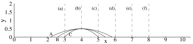
Figure 1: Sketch of the different bump geometries given by $y=-a\,(x-4)^{2}+0.5$ where $a$ is reported in table 1 and localisation of the different stations where statistics are addressed.

Five different simulations, whose parameters are summarised in table 1, have been carried out. Simulations A1, B1 and C1 have the same Reynolds number but different bump geometries, going from the most streamlined (A1) to the most bluff (C1) profile, see figure 1. A sketch of the whole three dimensional domain is shown in figure 3. Simulations A2 and A3 have the same bump geometry as simulation A1 but are performed at higher Reynolds numbers. Table 1 lists the nominal Reynolds number $Re$, the maximum friction Reynolds number $Re_{\tau}$ on the bump, the friction Reynolds number averaged on the top and bottom walls $\overline{\Rey_{\tau}}$ and the grid spacing in all directions. The grid is uniform in the streamwise and spanwise directions, and stretched in the wall normal direction to cluster grid nodes toward the walls, see table 1. The nominal Reynolds, $\Rey=h_{0}U_{b}/\nu$, is defined in terms of half the channel height, $h_{0}$, of the bulk velocity, $U_{b}$, and of the kinematic viscosity, $\nu$. The friction Reynolds number is $\Rey_{\tau}=hu_{\tau}/\nu$, with $u_{\tau}=\sqrt{\tau_{w}/\rho}$ the shear velocity ($\tau_{w}$ is the local mean shear stress and $\rho$ is the density), and $h$ half the local channel height. DNS is employed to solve the incompressible Navier-Stokes equations,

$$\frac{\partial u_{i}}{\partial t}+u_{j}\frac{\partial u_{i}}{\partial x_{j}}=-\frac{\partial p}{\partial x_{i}}+\frac{1}{Re}\frac{\partial^{2}u_{i}}{\partial x_{j}^{2}}\quad\quad\quad\frac{\partial u_{i}}{\partial x_{i}}=0,$$ (1)

where $u_{i}$ is the $i^{th}$ velocity component, and $p$ is the hydrodynamic pressure. Henceforth all length scales are made dimensionless with the nominal channel half-height, $h_{0}$, time scales with $h_{0}/U_{b}$ and pressures with $\rho U_{b}^{2}$.

The simulations are carried out using Nek5000, see Fischer et al. (2008), which is an open-source code that can simulate unsteady incompressible and low Mach number flows. The discretisation is based on the Spectral Element Method (SEM), see Patera (1984), whose formulation allows for Direct Numerical Simulations. Highly accurate numerical approaches for the simulation of wall bounded turbulent flows are crucial since it is desirable that the numerical error does not contaminate the multi-scale non-linear interactions. This feature is fulfilled by the SEM approach, which reconciles the high accuracy, typical of a spectral method, and the flexibility (in terms of geometrical configuration), typical of finite element approaches.

The grid spacing in the wall normal direction $y$ at the centre of the domain and at the walls is given by $\Delta{y^{+}}_{max}$ and $\Delta{y^{+}}_{min}$, respectively. The superscript $+$ denotes wall units referred to the average friction Reynolds number. The uniform grid spacing in the streamwise $x$ and spanwise direction $z$ in inner units is denoted by $\Delta{x^{+}}$ and $\Delta{z^{+}}$ respectively. These values, reported in table 1, are well within the grid resolution suggested by Kim et al. (1987) for well resolved DNS of wall bounded turbulent flows. Comparison of the local grid spacing, $\Delta=\sqrt[3]{\Delta x\Delta y\Delta z}$, with the local Kolmogorov scale, $\eta=\left(\nu^{3}/\epsilon_{T}\right)^{1/4}$ where $\epsilon_{T}$ is the turbulent kinetic energy dissipation rate, is shown in figure 2, in particular the quantity $\pi\eta/\Delta$ is reported for the highest Reynolds number case. The resolution requirement for a classical spectral method is $k_{max}\eta=\pi\eta/\Delta>1$. In the present case $\pi\eta/\Delta$ ranges between $1$ in the recirculation bubble and almost $3$ in the bulk of the flow, values adequate for the high fidelity reconstruction of the small scale dynamics of the flow, given the accurate dispersion characteristics of the spectral element method.

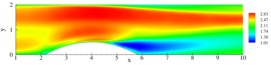
Figure 2: Kolmogorov scale with respect to the local grid spacing, $\pi\eta/\Delta$, for simulation A3, where $\Delta=\sqrt[3]{\Delta x\Delta y\Delta z}$.

The bump profile on the lower wall is generated using the equation $y=-a\,(x-4)^{2}+0.5$, where the coefficient $a$ is reported in table 1 for each simulation. The mesh for the lower Reynolds number case contains approximately 120 million grid points and the simulation was run on 8192 cores, using approximately 6 million core hours. The mesh for the higher Reynolds number case was run with approximately 400 million grid points on 32768 cores using approximately 30 million core hours. All simulations were run with a spectral element order $N=9$ except for the high Reynolds number simulation (A3) which was run at a spectral element order $N=11$. The reason for changing the spectral order is purely technical, motivated by the need of optimising the machine performance at changing dimensions of the simulation. All simulations were run on the FERMI Blue Gene/Q Tier0 system at the CINECA supercomputer centre in Bologna, Italy.

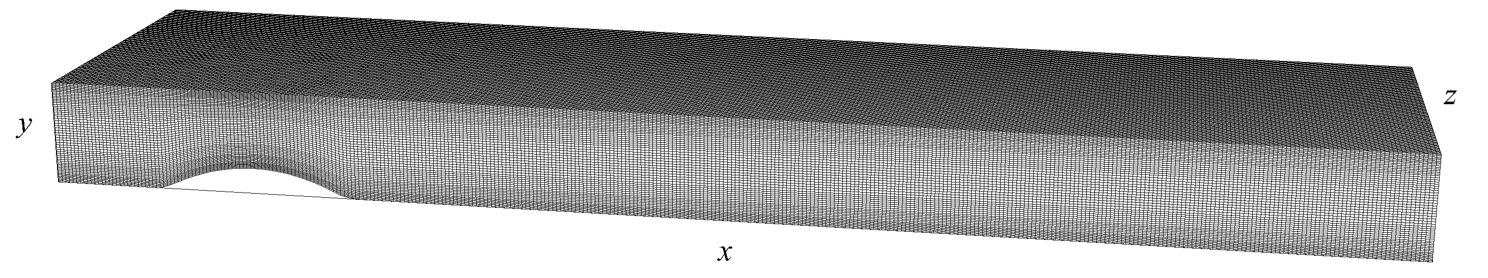
Figure 3: Sketch of the geometry of the channel with the curved lower wall for simulation (A). Periodic conditions are enforced in the streamwise, $x$, and spanwise, $z$, direction. No slip and impermeability are enforced on the top and bottom walls.

The geometry is shown in figure 3. The domain has dimensions $(L_{x}\times L_{y}\times L_{z})=(26\times 2\times 2\pi)$ to avoid flow confinement at high Reynolds number, see Lozano-Durán & Jiménez (2014) for similar issues in the context of planar channel flows. In the pictures, the flow is from left to right in the $x$ direction with periodic boundary conditions in both the $x$ and $z$ directions. No slip and zero normal velocity boundary conditions are imposed at the top and bottom walls. Accounting for periodicity, the actual geometry consists of an infinite channel with periodic bumps in the streamwise direction that are spaced by approximately 44 bump heights. The distance between consecutive bumps is enough to allow flow reattachment and to minimise the effects that the separation behind the fore bump may have on the aft bump. In this way, the use of inflow conditions, either synthetic or provided by companion channel simulations, is avoided. The flow is sustained by an overall pressure drop $\Delta p(t)$ in the $x$ direction that is modulated in time to keep the same constant flow rate for all simulations.

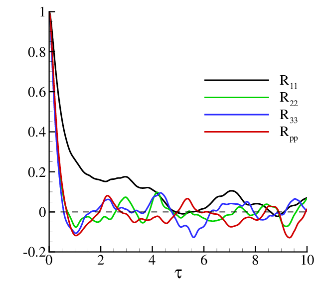
Figure 4: Temporal auto-correlation of velocity and pressure signals, for simulation A1, probed just after the bump at $x=5.8$ in panel (a) and at $x=24$ in panel (b). Panel (c) shows the spatial correlation of axial velocity fluctuations in the spanwise direction at $x=5.8$ and at $x=24$. All panels refer to the same distance from the upper planar wall, $d=2-y=1.6$. $\tau$ is normalised with $h_{0}/U_{b}$.

Approximately 500 statistically uncorrelated fields, separated by a time interval of $\Delta t_{stat}=6$, were collected for each simulation in order to obtain properly converging statistics. $\Delta t_{stat}$ is normalised with $h_{0}/U_{b}$. Defining the “flow-through time”, $t_{ft}$, as the time needed for a turbulent structure to travel all along the channel length, see Kähler et al. (2016), the simulation time is $T_{tot}=3000\simeq 115\,t_{ft}$, which makes sure that the velocity statistics converge (Kähler et al., 2016). Figure 4 shows, for simulation A1, the temporal auto-correlation of velocity,

$$R_{ii}(x,y,\tau) =\lim_{T\rightarrow\infty}\frac{1}{\pi T{u_{i}}_{\rm rms}^{2}}\int_{0}^{T}\int_{0}^{\pi}u^{\prime}_{i}(x,y,z,t)u^{\prime}_{i}(x,y,z,t+\tau)dzdt$$

$$=\frac{\langle u^{\prime}_{i}(x,y,z,t)u^{\prime}_{i}(x,y,z,t+\tau)\rangle}{{u_{i}}_{\rm rms}^{2}}\,,\qquad\mbox{no sum},$$

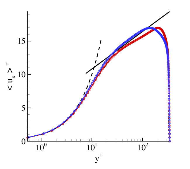
Figure 5: Plot of mean stream-wise (x-direction) velocity normalised with friction velocity, $\langle u_{x}\rangle^{+}=\langle u_{x}\rangle/u_{\tau}$, against $y^{+}$ at $x=24$ for simulations A1, A2 and A3 in panels (a), (b) and (c), respectively. The top and bottom wall velocities are represented by the blue and red lines, respectively. The dashed black line is the theoretical prediction, $\langle u_{x}\rangle^{+}=y^{+}$, in the viscous sub-layer. The solid black line is the theoretical prediction, $\langle u_{x}\rangle^{+}=1/k\,\log{(y^{+})}+A$, in the log-layer region with $k=0.41$ and $A=5.$

and pressure signals, $R_{pp}(x,y,\tau)=\langle p^{\prime}(x,y,z,t)p^{\prime}(x,y,z,t+\tau)\rangle/p_{\rm rms}^{2}$, probed at different locations inside the domain with the local root mean square fluctuation defined to normalise to one the correlation at zero time separation, i.e. $R_{ii}(x,y,0)=1$. Angular brackets indicate averages over the homogeneous coordinates, $z$ and $t$, while a prime indicates the fluctuation with respect to the local mean value. Some probes are located just beyond the bump (panel (a) of figure 4) and some others in the fully reattached flow (panel (b) of figure 4). The correlations confirm that fields separated by $\Delta t_{stat}$ are uncorrelated. For the same points, the spatial correlation of streamwise velocity fluctuations, $R_{xx}(x,y,\zeta)=\langle u^{\prime}_{x}(x,y,z,t)u^{\prime}_{x}(x,y,z+\zeta,t)\rangle/{u_{x}}_{\rm rms}^{2}$, in the spanwise direction, $z$, is shown in panel (c) of figure 4. The solid line refers to the correlation just beyond the bump whilst the dashed line refers to the correlation in the fully reattached flow. The spatial separation is normalised with (nominal) wall units $\zeta^{+}=\zeta\overline{\Rey_{\tau}}$. In the reattached flow region, the minimum correlation occurs at $\zeta^{+}\simeq 100$ assuring that the spanwise length is suitable to avoid confinement effects on the turbulent structures. Close to the bump, the correlation minimum occurs at $\zeta^{+}\simeq 80$. The inset in the figure reports the same quantities as a function of the spanwise separation normalised with the external unit.

Figure 5 shows plots of dimensionless mean stream-wise (x-direction) velocity, $\langle u_{x}\rangle^{+}=\langle u_{x}\rangle/u_{\tau}$, against $y^{+}=y\,\overline{\Rey_{\tau}}$ at $x=24$ averaged in the top half of the channel (blue) and in the bottom half (red), for simulations A1, A2 and A3. At this station, the flow almost entirely recovers the structure of a canonical turbulent channel flow. The plots show a well resolved viscous sub-layer, the buffer layer and the expected log-law region. The theoretical prediction for the viscous region close to the wall is represented by the dashed black line, $\langle u_{x}\rangle^{+}=y^{+}$. The symbols in the plots denote actual data points, showing the high resolution achieved in the simulation. The solid black line represents the log-law, $\langle u_{x}\rangle^{+}=1/k\log{y^{+}}+A$. The figure shows that, both at the bottom and top wall, this law is approached by the present data with better accuracy as the Reynolds number is increased, see the caption of the figure for the values of Von-Karman constant and intercept which are in agreement with those found in, e.g., Nagib & Chauhan (2008); Marusic et al. (2013).

3 Results

3.1 Instantaneous flow fields

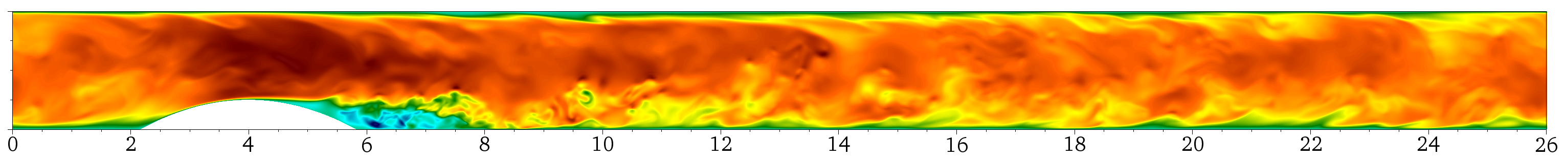
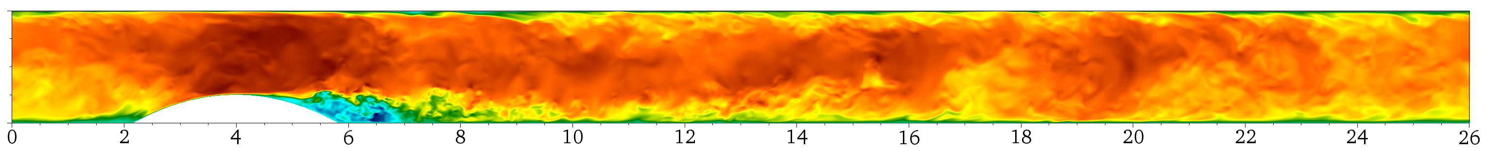
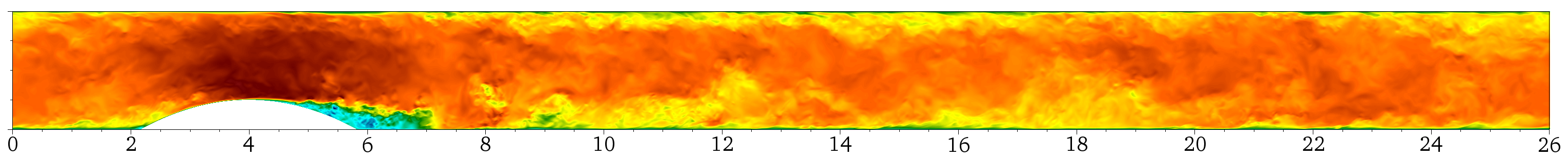
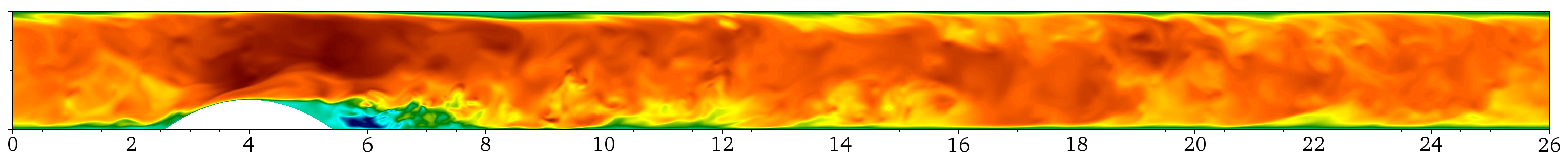
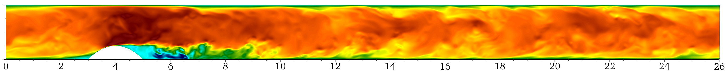
Figure 6: Instantaneous stream-wise velocity contour plots in x-y planes for all five simulations.

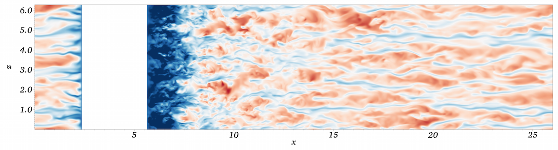
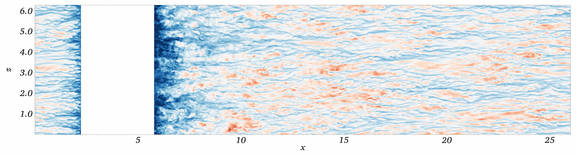
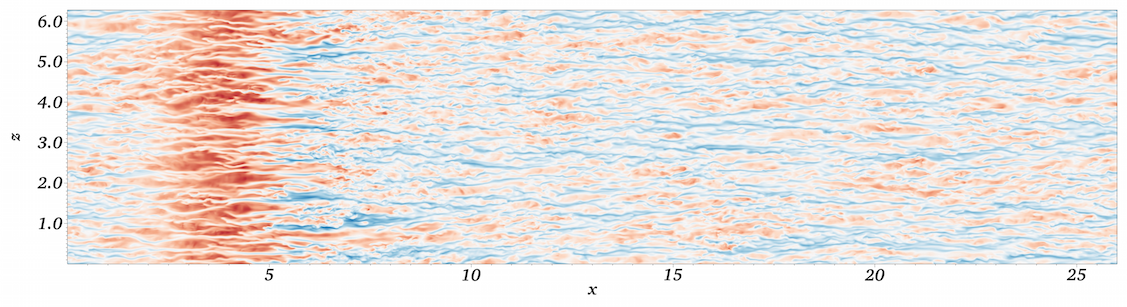
Figure 7: Instantaneous stream-wise velocity contour plots in x-z planes at $y^{+}=15$ in panels (a) and (b), $y=0.5$ in panels (c) and (d) and $y^{+}=15$ (from the top wall) in panels (e) and (f). Simulation A1 in panels (a), (c), (e) and simulation A3 in panels (b), (d) and (f).

Figure 6 shows instantaneous contour plots of streamwise velocity in the x-y plane for all the simulations. As expected, investing the bump, the flow velocity increases at the channel restriction and separates behind the bump with the formation of an intense shear layer between the bulk flow and the separation bubble close to the bottom wall. With increasing Reynolds number, cases A1, A2 and A3 progressively, structures at smaller scales appear. The separated region behind the bump becomes smaller, more attached to the bump and less protruded in the streamwise direction. It is interesting to compare, at least qualitatively, the flow snapshots for cases A1 and A3 with the smoke patterns used to visualise the boundary layer on a convex wall as shown in pg. 91 of the classical album by Van Dyke (1982). Indeed, in case A3 the flow impinging the bump is clearly characterised by small scale structures while case A1, even though nominally turbulent, appears smoother. Under this respect, case A3 can be regarded as producing a turbulent boundary layer between the external turbulent stream and the wall able to better withstand the adverse pressure gradients before separation. The separated region in front of the bump is also smaller at high Reynolds number. On the other hand, the separated region behind the bump becomes larger as the bump becomes bluffer. At the top wall, the boundary layer thickens after the constriction due to the adverse pressure gradient but separation is not observed. This effect is more evident for the lower Reynolds number cases, probably due to the higher extension of the recirculation bubble.

Figure 7 shows instantaneous contour plots of streamwise velocity in x-z planes at three wall normal distances for simulations A1 and A3 to qualitatively compare Reynolds number effects. At the higher Reynolds number, smaller structures are clearly present and the spacing between region of high and low speed is greatly reduced. In the far-downstream region and close to the walls, this is consistent with the expected scaling of streak spacing in internal units, Robinson (1991). In particular, panels (a) and (b) show xz-planes close to the bottom wall at $y^{+}=15$. This wall distance corresponds to the classical buffer layer of the channel flow. The empty region in the plot represents the intersection of the plane with the bump. The recirculation region behind the bump is characterised, at this distance from the wall, by negative velocity and small-scale structures. The size of the region where reverse flow occurs decreases when increasing the Reynolds number. Downstream, the small scale structures elongate in the flow direction and resemble the streaky structures found in turbulent planar channel flow. The xz-planes for simulations A1 and A3, in panels (c) and (d), respectively, just touch the top of the bump which is indicated by the continuous zero velocity line at $x=4$ in the contour plot. The acceleration of the flow just before the bump and its deceleration just behind can be observed. The small scale structures far away from the bump increase their length downstream. For simulation A3, the flow structures generated in the shear layer appear confined in a smaller region since the flow is more attached to the bump’s surface and the separated region protrudes less in the streamwise direction. Panels (e) and (f) show the xz-planes close to the top wall, at $y^{+}=15$. The effect of the bump on the velocity is still present and a clear velocity increase is seen at the bump’s location, due to the cross-section restriction. This is followed by a low velocity region corresponding to the end of the separation bubble at the opposite wall. In this region, the turbulent structures maintain a streamlined, streaky shape and no separated region is present.

3.2 Mean velocity and turbulent fluctuations

In the statistical analysis to follow, the average of a generic quantity $q$ is indicated with the angular brackets, $\langle q\rangle$, or with the capital letter, $Q$, according to convenience, while the fluctuation is indicated with the apex, $q^{\prime}$. Details of the recirculation bubble for all the simulations are shown in figure 8, providing the contour plot of the mean streamwise velocity $\langle u_{x}\rangle$ normalised with the bulk velocity. The black solid line highlights the zero isolines to better appreciate the mean flow reversal.

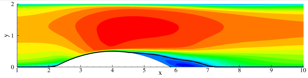
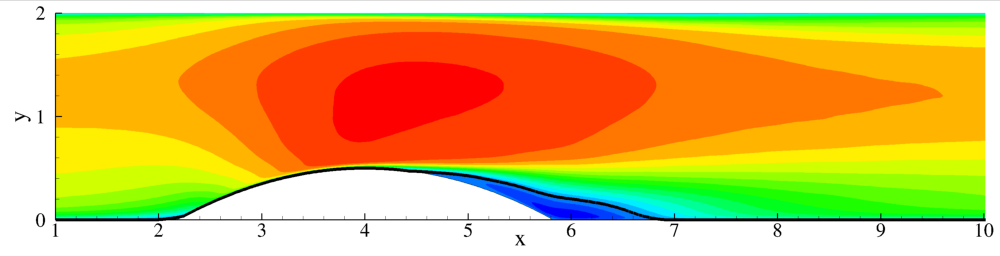
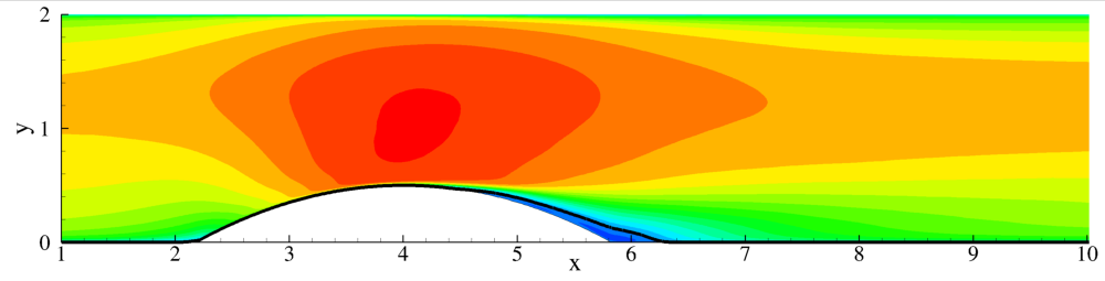
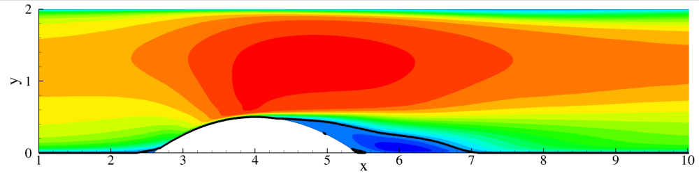
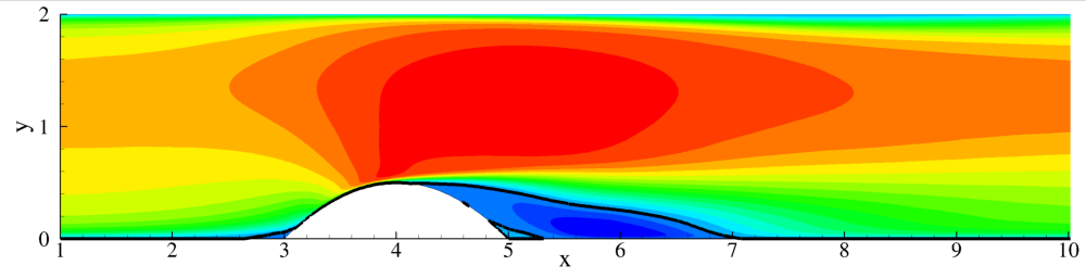
Figure 8: Average streamwise velocity $\langle u_{x}\rangle$ contour plots with isoline at $\langle u_{x}\rangle=0$ for all five simulations.

By progressively restricting the section, the first part of the bump makes the flow velocity increase consistently with the pressure decrease which is mechanically responsible for the acceleration. After the top of the bump the flow decelerates and a strong adverse pressure gradient occurs. This produces a backward flow near the bottom wall, giving rise to flow detachment. The bubble becomes smaller and more attached to the bump starting from the lower Reynolds number (A1) to the higher Reynolds number (A3). The profiles recuperate positive average velocity at the bottom wall behind the bump at an earlier x-position for simulation A3 compared to simulation A2 or A1. Concerning the effect of the geometry, the bubble becomes larger starting from the streamlined bump in simulation A1 to the more bluff geometry in simulation C1. However, the mean position of the reattachment point in the streamwise direction is basically independent of the bump width, at $x=7$ for all three geometries at $\Rey=2500$, while it clearly depends on the Reynolds number.

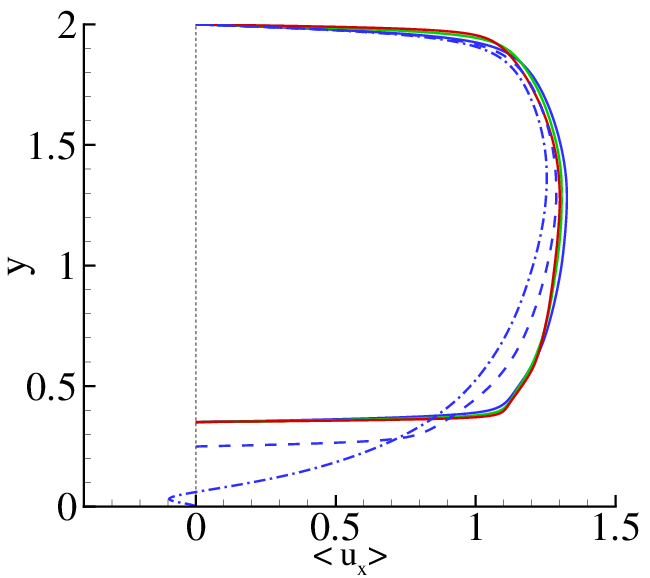
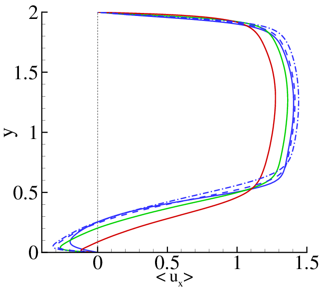
Figure 9: Mean axial velocity, $\langle u_{x}\rangle$, at six positions (a) to (f) corresponding to the stations in figure 1. Simulations A1, B1 and C1 are represented by solid, dashed and dashed-dotted blue lines respectively. Simulations A2 and A3 are represented by solid green and red lines respectively.

The above discussion is confirmed in detail by considering the mean velocity profiles extracted from figure 8 and reported in figures 9 and 10 at the downstream positions shown in figure 1. Simulations A1, B1 and C1 are represented by solid, dashed and dashed-dotted blue lines respectively whilst simulations A2 and A3 are represented by solid green and red lines respectively. Figure 9 shows mean streamwise velocity profiles for all five simulations. For the station shown in panel (a), the profiles are almost independent of the Reynolds number (solid lines) while they depend strongly on the geometry (broken lines), suggesting that the mean flow has already achieved a sort of asymptotic state. The profile for case C1 extends down to the bottom wall with a slightly negative velocity, indicating a small recirculating region ahead of the bump. At the tip of the bump, panel (b), all the profiles essentially exhibit the same behaviour. The recirculation is already well developed at the station of panel (c) for the bluffest bulge, case C1. Further downstream, panel (d), the wall-normal extension of the backward flow are well evident for all cases except for the highest Reynolds number (case A3), where the recirculation is more attached to the wall and extends less streamwise. Since the extension of the bubble is larger for the lower Reynolds number cases, it is still present at the station corresponding to panel (e). In contrast, reattachment already occurred for the higher Reynolds number (cases A2-A3). Further downstream, panel (f), the flow is attached for all conditions.

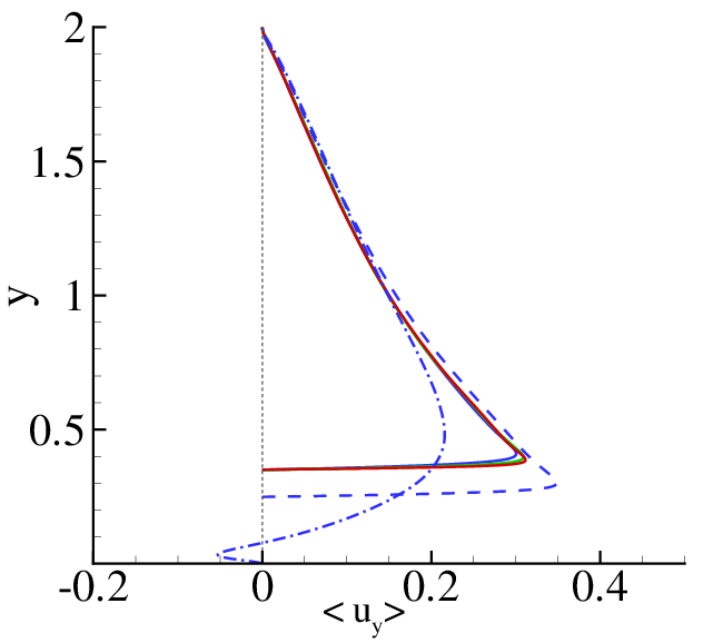
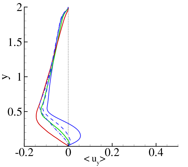
Figure 10: Mean wall-normal velocity, $\langle u_{y}\rangle$, at six positions (a) to (f) corresponding to the stations in figure 1. Simulations A1, B1 and C1 are represented by solid, dashed and dashed-dotted blue lines respectively. Simulations A2 and A3 are represented by solid green and red lines respectively.

Figure 10 shows the mean wall-normal velocity profiles. Wall-normal velocities are particularly intense as the flow invests the bump, panel (a). At the tip of the bump, panel (b), the positive (away from the bottom wall) wall-normal velocity peak is higher for the less streamlined bump (C1), indicating that the flow is strongly converging towards the opposite wall, leading to a contraction of the effective section (vena contracta). The wall-normal velocity is progressively reduced downstream, to eventually become negative. At intermediate stations, see e.g. panel (c), the wall-normal velocity is negative in the outer flow, indicating the trend toward reattachment to the lower wall. Approaching the wall, $\langle u_{y}\rangle$ becomes zero at the edge of the recirculation bubble. Inside the bubble $\langle u_{y}\rangle$ is positive, indicating that the profile is traversing the fore part of the bubble, recirculating clockwise. Moving further downstream, the external flow still moves toward the lower wall, but now the aft part of the bubble is reached, implying a negative wall-normal velocity also inside the bubble. Finally, the reattachment point is reached and the wall-normal average velocity tends to vanish in the entire channel section, starting to recover nearly parallel-flow conditions expected far away from the bump. The shorter bubble length leads to a more abrupt reattachment, as seen by the large negative wall-normal average velocity in the red plot of panel (c). The bluffest configuration induces an evident secondary recirculation bubble just below the primary one where the bump ends, see also figure 8. Note that in this figure a small bubble is also apparent just ahead of the bump.

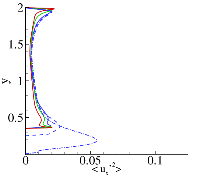
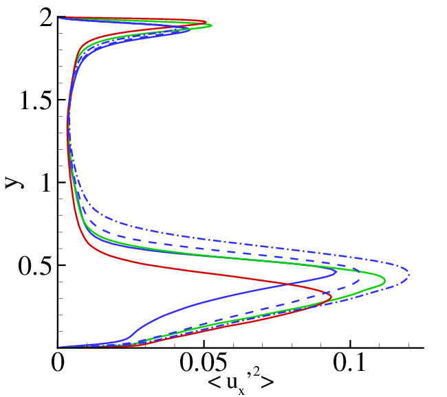
Figure 11: Mean streamwise velocity fluctuations, $\langle u_{x}^{\prime 2}\rangle$, at six positions (a) to (f) corresponding to the stations in figure 1. Simulations A1, B1 and C1 are represented by solid, dashed and dashed-dotted blue lines respectively. Simulations A2 and A3 are represented by solid green and red lines respectively.

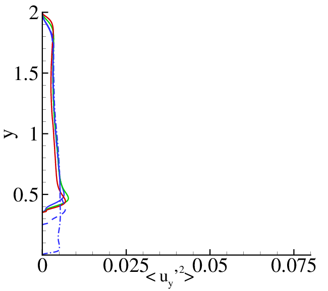
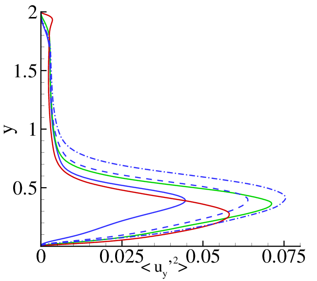
Figure 12: Mean wall-normal velocity fluctuations, $\langle u_{y}^{\prime 2}\rangle$, at six positions (a) to (f) corresponding to the stations in figure 1. Simulations A1, B1 and C1 are represented by solid, dashed and dashed-dotted blue lines respectively. Simulations A2 and A3 are represented by solid green and red lines respectively.

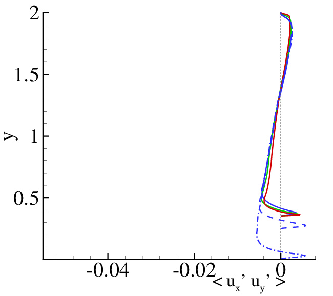
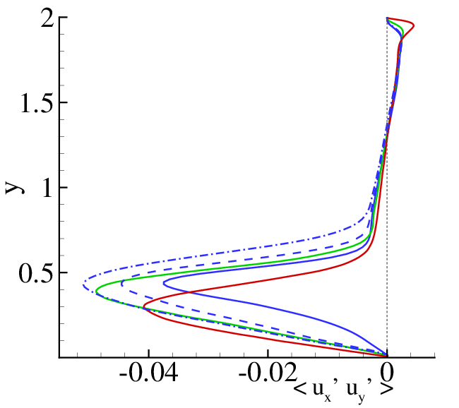
Figure 13: Reynolds stress, $\langle u_{x}^{\prime}u_{y}^{\prime}\rangle$, at six positions (a) to (f) corresponding to the stations in figure 1. Simulations A1, B1 and C1 are represented by solid, dashed and dashed-dotted blue lines respectively. Simulations A2 and A3 are represented by solid green and red lines respectively.

The next figures present the mean profiles for the fluctuating quantities, i.e. $\langle u_{x}^{\prime 2}\rangle$, $\langle u_{y}^{\prime 2}\rangle$ and $\langle u_{x}^{\prime}u_{y}^{\prime}\rangle$, at the same stations addressed above for the mean velocity profiles. Figure 11 shows mean streamwise velocity fluctuation profiles $\langle u_{x}^{\prime 2}\rangle$ for all five simulations. These are particularly strong close to the walls or inside the shear layer above the recirculating region, for all cases. The fluctuations are maximum in the high Reynolds number case (A3) and in the most bluff case (C1). In the former, the high velocity fluctuations are due to the higher Reynolds number, whilst in the latter, the fluctuations are fed by the strong flow separation induced by the bump shape. In the lower Reynolds number simulations, the regions with higher velocity fluctuations are larger, corresponding to a larger shear layer. The presence of the bump also results in an increase in fluctuations at the top wall, particularly evident for the lower Reynolds number simulations. The change in geometry also affects the maxima reached by the fluctuations. In particular, due to the increased size of the recirculating region, simulation C1 exhibits peak values which are comparable to simulation A3 in the shear layer, see panel (c). In correspondence of the recirculating region, the peaks are higher for case C1 with respect to the cases at the same Reynolds number, B1 and A1. The profiles for the wall-normal velocity fluctuations $\langle u_{y}^{\prime 2}\rangle$ and the Reynolds stress, $\langle u_{x}^{\prime}u_{y}^{\prime}\rangle$, follow a similar trend. The profiles are shown in figure 12 and figure 13 for all five simulations. The positive values of Reynolds stress confirm the presence of the small recirculation bubble ahead of the bump, panel (a) in figure 13.

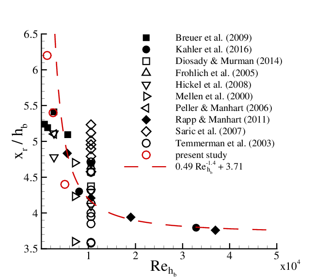
Figure 14: Dependence of the reattachment point normalised with the height of the obstacle $x_{r}/h_{b}$, on the Reynolds number based on $h_{b}$, $\Rey_{h_{b}}=\Rey\,h_{b}$. $h_{b}$ is the bump height normalised with the nominal channel half-height, $h_{0}$. Closed black symbols refer to experimental measurements, open black symbols to numerical simulations (mainly LES). Red dashed line is the exponential fit of the experimental data Kähler et al. (2016). Open red symbols are extracted from the present DNSs. Breuer et al. (2009), Kähler et al. (2016), Diosady & Murman (2014), Fröhlich et al. (2005), Hickel et al. (2008), Mellen et al. (2000), Peller & Manhart (2006), Rapp & Manhart (2011), Šarić et al. (2007), Temmerman et al. (2003)

The position of the reattachment point clearly does not depend on the dimension of the obstacle in the streamwise direction, but on the Reynolds number. These observations are in agreement with both numerical and experimental data already available in the literature. Figure 14 shows the reattachment point normalised with the height of the bump, $x_{r}/h_{b}$ as a function of the Reynolds number based on the bulk velocity and on the height of the bump, $\Rey_{h_{b}}=\Rey\,h_{b}$ (note that $h_{b}$ is the dimensionless bump height). Data have been collected in Kähler et al. (2016) from several experiments (closed symbols) and numerical simulations, mainly LES, (open symbols), whilst the open red circles are the present simulations.

Note that the geometries in these experiments and simulations only qualitatively corresponds to ours. We therefore focus the comparison on the re-attachment point whose position is mainly controlled by bump height and Reynolds number, quite independently of the detailed geometry. The red dashed line in the figure is a power-law fit, based on all experimental results, which asymptotically reaches $3.71\,x/h_{b}$ for large Reynolds numbers. The reattachment location scales with $\Rey_{h_{b}}$ to the power $-1.4$. The reattachment position moves further upstream with increasing Reynolds number due to the stronger turbulent mixing, i.e. due to a higher turbulent momentum transfer towards the wall. The present DNS data agree well with the experimental results of Kähler et al. (2016) and of Rapp & Manhart (2011). Overall, this compilation of data shows a significant scatter of data obtained by turbulence modeling and a certain inability of the models to capture the bubble reattachment position, see also the discussion in Kähler et al. (2016) for more details. Concerning the present DNS, the slight differences with the experiments can be attributed to details of the turbulence investing the bump and the confinement effect of the upper wall.

3.3 Pressure, drag and friction coefficients

The instantaneous pressure is decomposed as the sum of a contribution linearly decreasing in the streamwise direction, which is associated to the instantaneous pressure drop $\Delta p(t)$ across the channel, plus a departure $\tilde{p}$ from the linear law,

$$p({\bf x},t)=-\frac{\Delta p}{L_{x}}x+{\tilde{p}}({\bf x},t)\ .$$

In the present simulations $\Delta p(t)$ does not significantly fluctuate in time, oscillating within 1% at most, although its value is in principle continuously adjusted to keep the flow rate rigorously constant. The drag coefficient in terms of the present dimensionless variables is

$$C_{d}=4\frac{\Delta P}{L_{x}}=-\frac{2}{L_{x}}\int_{walls}\langle{\bf t}\rangle\cdot{\bf e}_{x}dl\,,$$

where $\Delta P=\langle\Delta p\rangle$ is the average pressure drop, $\bf t$ is the (dimensionless) traction at the wall (pressure plus shear force) and ${\bf e}_{x}$ is the unit vector in the streamwise direction. Wherever needed (see e.g. §3.4.2) the fluctuation of the pressure drop will be denoted by $\Delta p^{\prime}(t)$.

The drag increases moving from the most streamlined (A1) to the most bluff profile (C1), see table 2. On the other hand, the drag coefficient decreases with the increase in Reynolds number, from simulation A1, A2 to A3. For purpose of comparison, the drag in a planar channel at the same flow rate is $C_{d}^{channel}=4\left(\Rey_{\tau}^{0}/\Rey_{b}\right)^{2}$. The drag coefficient can be decomposed in form and friction components, namely

$$C_{d}^{form}=\frac{2}{L_{x}}{\bf e}_{x}\cdot\int_{walls}P\,{\bf n}\,dl\,,\qquad C_{d}^{friction}=-\frac{2}{L_{x}}{\bf e}_{x}\cdot\int_{walls}\mu\,\frac{\partial{\bf U}}{\partial n}dl\,,$$

where ${\bf n}$ is the unit normal exiting the fluid domain. The form drag coefficient increases by $50\%$ going from the most streamlined to most bluff shape. The observed decrease of the form drag coefficient with increasing Reynolds number is more than compensated by the larger velocity for flows in the same geometry implying, as obvious, the increase of the corresponding contribution to the resistance, $D^{form}\propto U_{b}^{2}C_{d}^{form}$. In the present geometry, the friction component is dominated by the straight part of the channel and its value is not significantly different from the one expected in a planar channel, see the small difference $C_{d}^{friction}-C_{d}^{channel}$ in table 2. This confirms that most of the bump-induced drag should be interpreted as form drag.

Case		$C_{d}$		$C_{d}^{form}$		$C_{d}^{channel}$		$C_{d}^{friction}-C_{d}^{channel}$
$A1$		$3.07\cdot 10^{-2}$		$1.06\cdot 10^{-2}$		$1.80\cdot 10^{-2}$		$0.21\cdot 10^{-2}$
$B1$		$3.26\cdot 10^{-2}$		$1.28\cdot 10^{-2}$		$1.80\cdot 10^{-2}$		$0.18\cdot 10^{-2}$
$C1$		$3.49\cdot 10^{-2}$		$1.55\cdot 10^{-2}$		$1.80\cdot 10^{-2}$		$0.14\cdot 10^{-2}$
$A2$		$2.68\cdot 10^{-2}$		$1.05\cdot 10^{-2}$		$1.44\cdot 10^{-2}$		$0.19\cdot 10^{-2}$
$A3$		$2.05\cdot 10^{-2}$		$7.07\cdot 10^{-3}$		$1.17\cdot 10^{-2}$		$0.17\cdot 10^{-2}$

Table 2: Drag coefficient decomposed into form and friction contributions and comparison against an equivalent planar channel. See text for definitions.

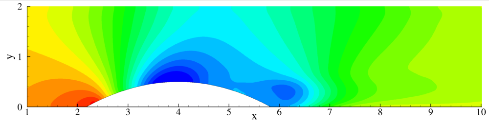
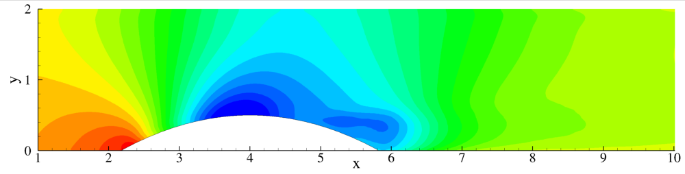
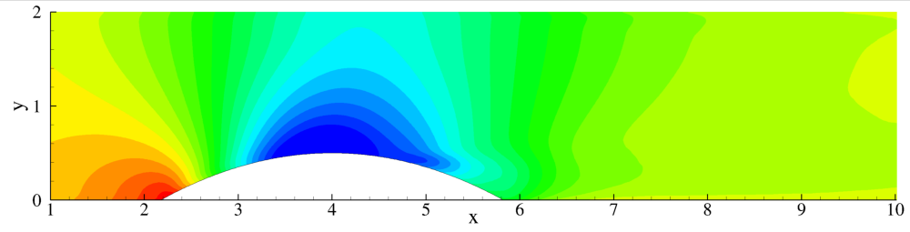
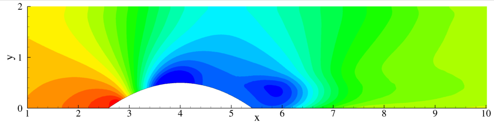
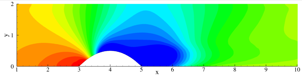
Figure 15: Average pressure $\langle p\rangle$ contour plots for all five simulations.

Given its relevance in determining the drag, the mean pressure field is shown in figure 15 for all simulations. Roughly, the qualitative behaviour is similar for all cases. A high pressure region occurs just before the bump where a stagnation point occurs. Further downstream the pressure decreases reaching its minimum in the high velocity region, at the top of the bump. The pressure field behind the bump is strongly influenced by the shape and dimension of the recirculation bubble. When the separation region is significant, cases A1, B1 and C1, a second pressure minimum develops inside the recirculation bubble. The high Reynolds number simulations where performed on the most streamlined geometry, which produces a smaller separation compared to the other geometries. With increasing Reynolds number, cases A2 and A3, the flow more easily faces the adverse pressure gradient due to enhanced turbulent mixing, resulting in delayed separation. As a consequence, pressure recovery behind the bump is more effective.

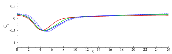
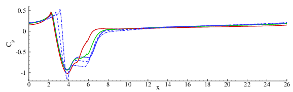
Figure 16: Modified pressure coefficient at the top and bottom walls of the domain, top and bottom panels respectively. Simulations A1, B1 and C1 are represented by solid, dashed and dashed-dotted blue lines respectively. Simulations A2 and A3 are represented by solid green and red lines respectively.

Given the average pressure drop along the channel, the effect of the bump on the wall pressure is better addressed in terms of a departure-pressure coefficient

$$C_{p}^{t/b}(x)=\left.2\,\langle{\tilde{p}}\rangle\right|_{y=2/y=0}\,,$$

where the superscripts ‘$t$’ and ‘$b$’ refer to the top and bottom wall respectively. Adding the linear term $-2x\Delta P/L_{x}$ recovers the standard definition of $C_{p}$. Figure 16 shows the departure-pressure at both walls. The effect of the bump extends to the opposite wall, with $C_{p}^{t}$ presenting a trough just after the bump tip (at $x=4$) and recovering downstream. The trough is smaller and shifted closer to the bump tip with increasing Reynolds number. At constant Reynolds number, the trough is more pronounced and farther away from the tip when the geometry is bluffer, i.e. simulations B1 and C1. At the bottom wall, as the flow reaches the bump, $C_{p}^{b}$ initially increases producing a small recirculation just ahead of the bump. The pressure then decreases to its minimum slightly ahead of the tip. These trends become stronger for the bluffer geometries. Immediately downstream of the tip, the pressure abruptly rises reaching the separation point. In the recirculation bubble the pressure remains almost constant, with the extension of the plateaux becoming smaller at increasing Reynolds number (red line). The extension of the plateaux is almost independent of the geometry, where $C_{p}^{b}$ decreases for bluffer bumps.

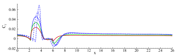
Figure 17: Mean skin friction coefficient along $x$ at the top and bottom walls of the domain in the top and bottom panels respectively. Simulations A1, B1 and C1 are represented by solid, dashed and dashed-dotted blue lines respectively. Simulations A2 and A3 are represented by solid green and red lines respectively.

Figure 17 shows the mean skin friction coefficient $C_{f}=2\,\tau_{w}$. At the top wall, $C_{f}$ is always positive, showing that the adverse pressure gradient (see figure 16) is too mild to induce average flow separation on the wall opposite to the bump. The maximum and minimum $C_{f}$ occur just before the bump tip and at the end of the bubble, respectively. At the bottom wall, the skin friction coefficient ahead of the bump becomes slightly negative due to the small recirculation bubble and reaches a positive peak as the flow approaches the tip of the bump. For the different Reynolds numbers, the position of the peak coincides but the maximum reduces with increasing Reynolds number. The peak is shifted towards the tip with increasing bluffness of geometry. A skin friction plateaux is observed behind the tip, along the bump where the cross-stream section of the channel increases. At the bubble, consistently with the backward flow at the wall, the skin friction is negative, with increasing absolute value for bluffer geometries and lower Reynolds numbers.

3.4 Mean kinetic energy and turbulent kinetic energy budgets

The Reynolds decomposition entails the splitting of the total kinetic energy in two parts, $K=K_{M}+k_{T}$, where $K_{M}=1/2\,\langle u_{i}\rangle\langle u_{i}\rangle$ is the kinetic energy of the mean flow and $k_{T}=1/2\langle u^{\prime}_{i}u^{\prime}_{i}\rangle$ is the turbulent kinetic energy. In literature, little attention is typically paid to the kinetic energy of the mean field and most interest is focused on the turbulent contribution. This is motivated by the usually simple flow configuration where the mean balance equation for $K_{M}$ is trivial. In the present case both mean and turbulent kinetic energy need to be dealt with explicitly. The reason is that the bump breaks the streamwise homogeneity and induces strong mean wall-normal velocities. This gives rise to non-trivial mean and turbulent spatial energy fluxes, dissipation, and turbulent kinetic energy production.

3.4.1 Mean kinetic energy

The (stationary) mean flow kinetic energy equation reads

$$\frac{\partial{\Phi_{M}}_{j}}{\partial x_{j}}=-\varepsilon_{M}-{\Pi}+\frac{\Delta P}{L_{x}}U_{x}\,,$$ (2)

where $\varepsilon_{M}=1/\Rey(\partial U_{i}/\partial x_{j})(\partial U_{i}/\partial x_{j})$ is the mean flow energy dissipation rate per unit volume and ${\Pi}=-\langle u^{\prime}_{i}u^{\prime}_{j}\rangle{\partial U_{i}}/{\partial x_{j}}$ is the turbulent kinetic energy production. ${U_{x}\Delta P}/{L_{x}}$ is the external average power input. The spatial flux,

$${\Phi_{M}}_{j}=U_{j}K_{M}+{U_{j}\langle{\tilde{p}}\rangle}-\frac{1}{\Rey}\frac{\partial K_{M}}{\partial x_{j}}+U_{i}\langle u^{\prime}_{i}u^{\prime}_{j}\rangle\,,$$ (3)

redistributes energy across the flow, overall providing zero net contribution to the power.

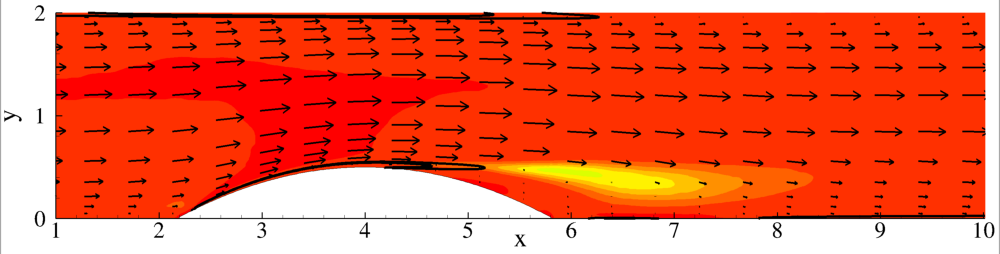
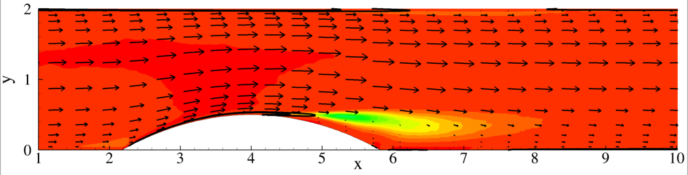
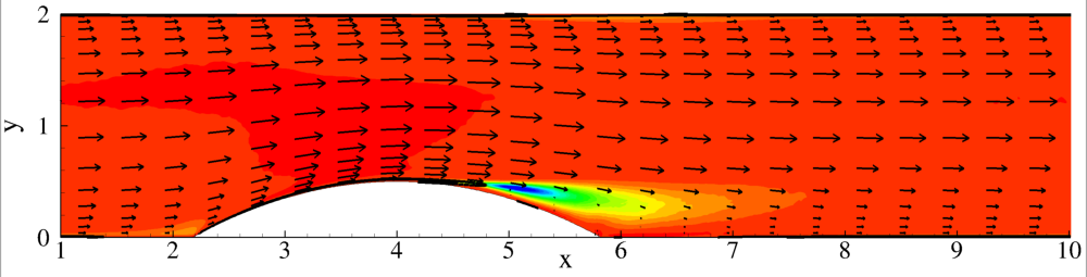
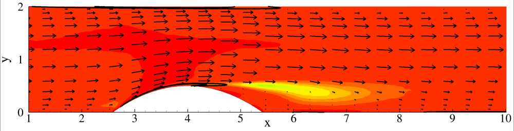
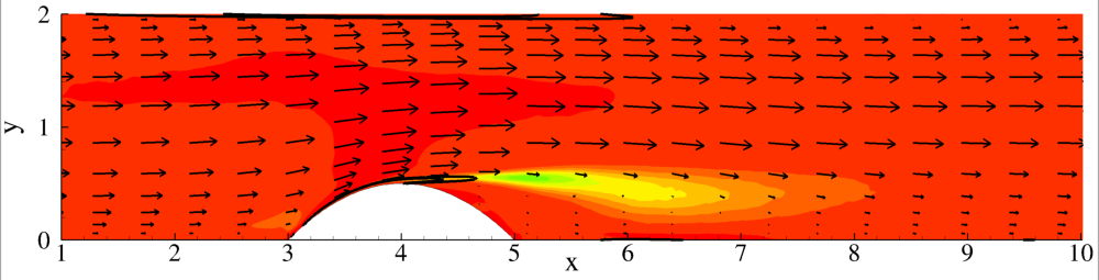
Figure 18: Mean kinetic energy balance equation: turbulent kinetic energy production $-\Pi$ (background colour), mean energy dissipation $\varepsilon_{M}$ (solid isolines) and mean energy spatial flux $\Phi_{M}$ (vectors).

Figure 18 shows the terms in equation (2) normalised with the total average power injection per unit volume, i.e. the total dissipation rate, $\int\left(\varepsilon_{M}+\varepsilon_{T}\right)dV$ where $\varepsilon_{T}=\langle 1/\Rey(\partial u^{\prime}_{i}/\partial x_{j})(\partial u^{\prime}_{i}/\partial x_{j})\rangle$ is the turbulent dissipation rate density. In the figure, the turbulent kinetic energy production rate, $-\Pi$, is shown in the background colour plot whilst solid isolines (mostly concentrated near the bump wall) represent the mean field dissipation, $\varepsilon_{M}$. Vectors correspond to the spatial flux $\Phi_{Mj}$.

Given the behaviour of the mean streamwise velocity, see figure 8, the mean energy input, ${U_{x}\Delta P}/{L_{x}}$, is largest at the bump tip. On the other hand, the production $-\Pi$, is concentrated in the detaching shear layer well behind the bump, where the largest fluctuation intensities are attained, as discussed in the previous section. This region acts as a sink of mean energy and is fed by the mean energy flux, ${\Phi_{M}}_{j}$, that is crucial in redistributing energy from the external input to the turbulent production. With respect to case A1, taken as a basis for comparison, the maximum turbulent production increases by almost 50% for the bluffer geometry and by 400% at the maximum Reynolds number. By definition, turbulent production is the product of mean flow gradients and Reynolds stresses. For the given geometry, the mean gradients in the shear layer slightly depend on Reynolds number, as shown in panel (c) of figure 9 which corresponds to the section of maximum production. This suggests that the mean field already attained an almost Reynolds independent state. On the other hand, turbulent stresses increase significantly at this section, see panel (c) of figure 13, resulting in the increased peak production apparent in figure 18. In general, the position of the energy production region depends, through the shear layer, on the dimensions and the position of the separation bubbles. Changing geometry at fixed, lower Reynolds number, the strength of the mean gradients in the same section, now in panel (d) of figure 9, are only marginally affected by the change in geometry. On the other hand, the Reynolds stresses are greatly enhanced passing from a streamlined to a bluff configuration, panel (d) in figure 13, consistent with the increasing peak energy production from case A1 to case C1 in figure 18.

Although hardly apparent in figure 18, for the considered cases the mean flow dissipation rate is not irrelevant, and contributes order 40% of the total dissipation in the system, consistently with significant mean velocity gradients, observed at the bump wall where the flow is abruptly accelerated.

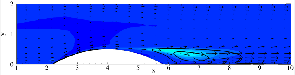
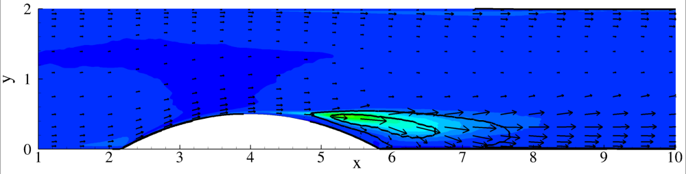
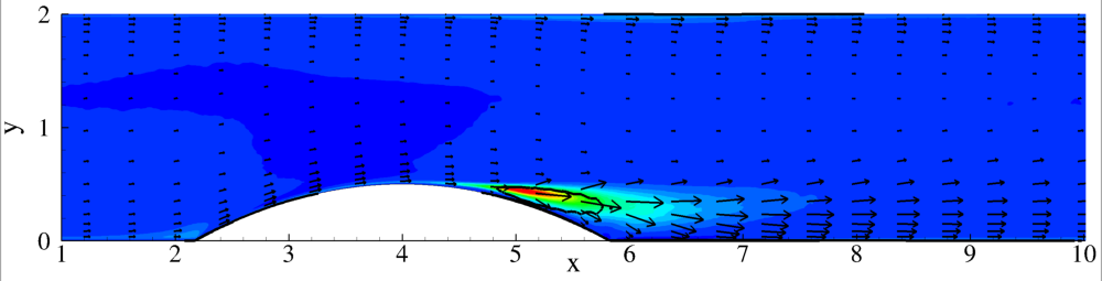
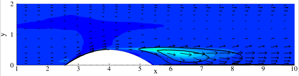
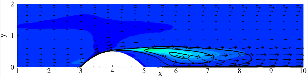
Figure 19: Turbulent kinetic energy balance equation: turbulent kinetic energy production $\Pi$ (background colour), turbulent energy dissipation $\varepsilon_{M}$ (solid isolines) and turbulent energy spatial flux $\Phi_{M}$ (vectors).

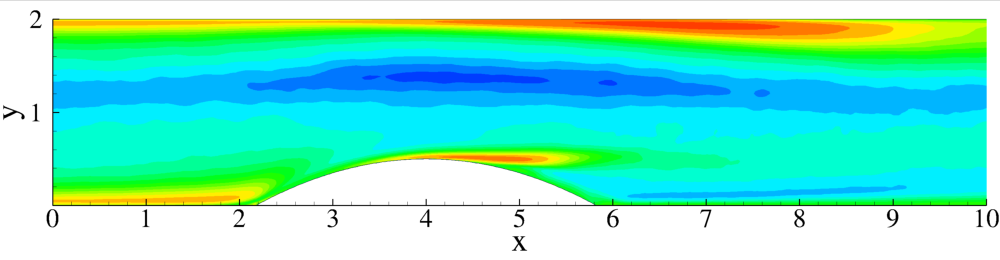
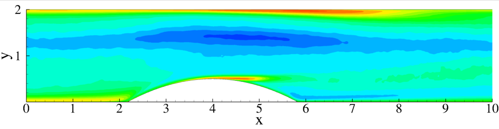
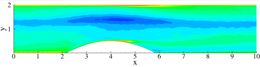
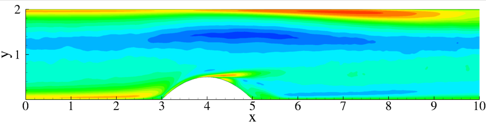
Figure 20: Norm of the deviatoric component of the Reynolds stress tensor, $||b||=\sqrt{b_{ij}b_{ij}}$ with $b_{ij}=\langle u^{\prime}_{i}u^{\prime}_{j}\rangle/\langle u^{\prime}_{k}u^{\prime}_{k}\rangle-1/3\,\delta_{ij}$, and $\delta_{ij}$ the components of the identity tensor.

3.4.2 Turbulent kinetic energy

The balance equation for the turbulent kinetic energy reads

$$\frac{\partial\Phi_{Tj}}{\partial x_{j}}=-\varepsilon_{T}+{\Pi}+\langle\frac{\Delta p^{\prime}(t)}{L_{x}}\,u^{\prime}_{x}\rangle\,,$$ (4)

where, as anticipated, $\varepsilon_{T}$ is the turbulent kinetic energy dissipation rate, $\Pi$, here with the opposite sign with respect to eq. (2), is the production and $\langle\Delta p^{\prime}\,u^{\prime}_{x}/L_{x}\rangle$ is the external source of fluctuating energy. The spatial flux,

$$\Phi_{Tj}=U_{j}k_{T}+\frac{1}{2}\langle u^{\prime}_{i}u^{\prime}_{i}u^{\prime}_{j}\rangle+{\langle\tilde{p}^{\prime}u^{\prime}_{j}\rangle}-\frac{1}{\Rey}\frac{\partial k_{T}}{\partial x_{j}}\,,$$ (5)

contributes zero net power when integrated over the whole domain. The energy locally provided by the fluctuations of pressure difference between inlet and outlet $\langle\Delta p^{\prime}\,u^{\prime}_{x}/L_{x}\rangle$ is negligible, $\max\limits_{x,y}{\langle\Delta p^{\prime}\,u^{\prime}_{x}/L_{x}\rangle}\simeq 10^{-5}\,\max\limits_{x,y}\Pi$.

Figure 19 shows the turbulent kinetic energy production, turbulent energy dissipation and spatial fluxes for all the simulations. The terms are normalised with the overall power injected in the system which, in the statistically steady state, is balanced by the total dissipation rate, $\int\left(\varepsilon_{M}+\varepsilon_{T}\right)dV$. The production term injects most energy in the shear layer behind the bump. From the shear layer the energy follows different paths, see the vector field in the figure where local energy release is associated with the (positive) divergence of the energy flux. The turbulent energy is transferred towards the centre of the channel, into the separation bubble or towards the wall, in particular behind the bump under the separation bubble. From the analysis of the dissipation field, $\varepsilon_{T}$, part of the energy is found to be locally dissipated in the shear layer and in the separation bubble. Most of the energy is dissipated at the bottom wall after the bump (note the isolines of dissipation concentrated in that region).

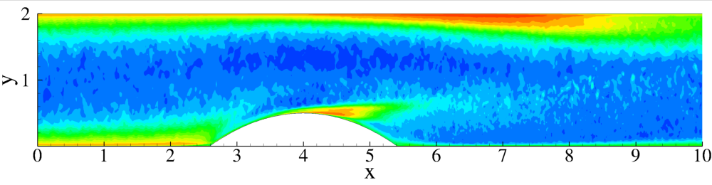
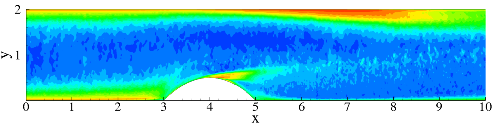
Figure 21: Norm of the deviatoric component of the pseudo dissipation tensor, $||d||=\sqrt{d_{ij}d_{ij}}$, where $d_{ij}=\epsilon_{ij}/\epsilon_{kk}-1/3\,\delta_{ij}$ and $\epsilon_{ij}=2/\Rey\langle\left(\partial u^{\prime}_{i}/\partial x_{k}\right)\left(\partial u^{\prime}_{j}/\partial x_{k}\right)\rangle$ is the pseudo dissipation tensor.

3.4.3 Large and small scale anisotropy

The anisotropy of the large turbulent scales is described by the deviatoric component of the Reynolds stress, $b_{ij}=\langle u^{\prime}_{i}u^{\prime}_{j}\rangle/\langle u^{\prime}_{k}u^{\prime}_{k}\rangle-1/3\delta_{ij}$, where $\delta_{ij}$ denotes the Kronecker symbol. Note that in isotropic conditions, $b_{ij}$ is identically zero. An overall measure of anisotropy is given by the norm $||b||=\sqrt{b_{ij}b_{ij}}$, figure 20. The anisotropy is particularly significant in the near wall region and in the shear layer, while the bulk flow and the recirculation bubble are almost isotropic, consistent with the Reynolds stress profiles of figures 11, 12 and 13. Increasing the Reynolds number, the anisotropic regions become progressively smaller, squeezed closer to the wall, on one side, and more concentrated in the shear layer, on the other. The extension of the isotropic region in the bulk widens, whilst it shrinks with the recirculation bubble in the separated region. As a result of the change in geometry, the bluffest bump produces the highest anisotropic content.

Figure 21 reports the norm, $||d||=\sqrt{d_{ij}d_{ij}}$, of the deviatoric component, $d_{ij}=\epsilon_{ij}/\epsilon_{kk}-1/3\,\delta_{ij}$, of the pseudo-dissipation tensor, $\epsilon_{ij}=2/\Rey\langle(\partial u^{\prime}_{i}/\partial x_{k})(\partial u^{\prime}_{j}/\partial x_{k})\rangle$. $||d||$ provides a measure of the small scale anisotropy content (Antonia et al., 1994; Pumir et al., 2016) and therefore, as $||d||$ approaches zero, isotropic behaviour of the smallest scales is achieved. The small scales in the recirculation bubble and in the bulk of the flow are isotropic, consistently with the isotropy of the large scales in the same regions. Strong anisotropy persists in the near wall regions and in the shear layer. The behaviour of $||d||$ is strongly dependent on the Reynolds number which ultimately sets the separation between the largest and the smallest scales. The regions of small-scale isotropy progressively increase with the Reynolds number, basically due to the shrinking of the large scale anisotropy regions. However, anisotropy still persists at small scales, irrespectively of the Reynolds number, near the walls and in the shear layer. This behaviour can be explained and understood by addressing the dynamics of a turbulent flow in presence of strong shear. In isotropic conditions the turbulence is forced at the largest scales comparable with the integral scale $L_{0}=(2k_{T})^{3/2}/\epsilon_{T}$ and is dissipated by viscosity at the Kolmogorov scale $\eta=(\nu^{3}/\epsilon_{T})^{1/4}$. In the inertial range ($\eta\ll r\ll L_{0}$) the energy is simply transferred from the large to the small scales. In turbulent shear flows the shear scale $L_{S}=\sqrt{\epsilon_{T}/S^{3}}$, extensively discussed in Casciola et al. (2003), where $S$ is the shear rate, plays a crucial role in explaining the dynamics. Basically the shear scale identifies the range of scales $L_{S}<r<L_{0}$ where the turbulence is driven by the (anisotropic) production of turbulent kinetic energy due to the Reynolds stresses. In the range of scales below $L_{S}$, $\eta<r<\L_{S}$, the dynamics of the turbulent fluctuations are driven by the process of energy cascade typical of isotropic flows, see e.g. Marati et al. (2004); Cimarelli et al. (2013) for a detailed analysis of the energy paths in a planar channel. It follows that the dynamics of a shear flow is described by two dimensionless parameters. The first one is the shear intensity $S^{*}=S\,(2k_{T})/\epsilon_{T}$, see e.g. Lee et al. (1990), that can be recast in terms of the shear scale as $S^{*}=\left(L_{0}/L_{S}\right)^{2/3}$, (Casciola et al., 2007). The shear intensity measures the separation between the shear scale and the integral scale thus providing the extension of the range of scales directly affected by the production mechanisms. The second parameter is the Corrsin parameter $S_{c}=S\sqrt{\nu/\epsilon_{T}}$ (Corrsin, 1958) that can be recast in terms of the shear scale as $S_{c}=\left(\eta/L_{S}\right)^{2/3}$. The Corrsin parameter measures the extension of the range between the shear scale and the Kolmogorov scale where the flow is driven by the inertial cascade. Clearly, only in the range of scales below the shear scale isotropisation of turbulent fluctuations can take place. The shear scale can be evaluated in spatially non homogeneous flows by considering the norm of the local mean velocity gradient $L_{S}=\sqrt{\epsilon_{T}/\left(\partial_{j}U_{i}\partial_{j}U_{i}\right)^{3/2}}$. In our case the shear scale is a field $L_{S}(x,y)$. In a similar way the local integral scale $L_{0}=(2k_{T})^{3/2}/\epsilon_{T}$ and the local Kolmogorov scale $\eta=(\nu^{3}/\epsilon_{T})^{1/4}$ can be considered. The shear strength $S^{*}$ and the Corrsin parameter $S_{c}$ are position dependent. When $S^{*}$ is large the whole range of scales is dominated by production and there is no room left for isotropy recovery at small scales. On the contrary, an isotropy recovery range is available where the Corrsin parameter is small. Figures 22 and 23 provide the fields $S^{*}$ and $S_{c}$ respectively, for the different Reynolds numbers and geometries considered in this paper. A joint analysis of $S^{*}$ and $S_{c}$ provides the physical interpretation of the observed anisotropy (figures 20 and 21). In the bulk region, $S^{*}$ decreases, denoting weak production of turbulent kinetic energy since the shear scale approaches the integral scale. Concurrently, $S_{c}$ is small, indicating a large separation between shear and Kolmogorov scale. This behaviour is generic and the only relevant changes are observed when the Reynolds number is increased, A1-A3. At large Reynolds number, the spatial region in the bulk where isotropisation occurs is broadened. The relative position of integral, shear and Kolmogorov scales in the bulk explains why the small scales are isotropic (figure 21). The conditions are different near the wall and in the shear layer. In these regions, see figure 22, $S^{*}$ is large and the whole range of scales is now dominated by turbulent kinetic energy production. Concurrently $S_{c}$ is order one, i.e. the shear scale is forced on the Kolmogorov scale (figure 23). This behaviour is again generic for the cases we address. In a nutshell, near the wall and in the shear layer there is no room for the formation of the inertial range where isotropisation can take place. The flow is driven by the anisotropic mechanisms of turbulent kinetic energy production, see figure 20 and the anisotropy persists down to the smallest scales (figure 21).

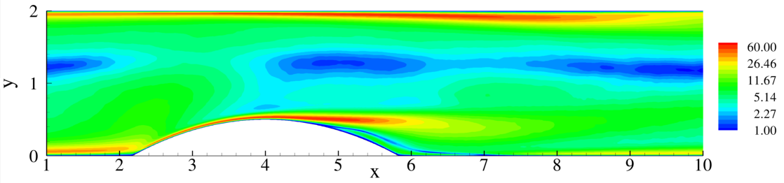
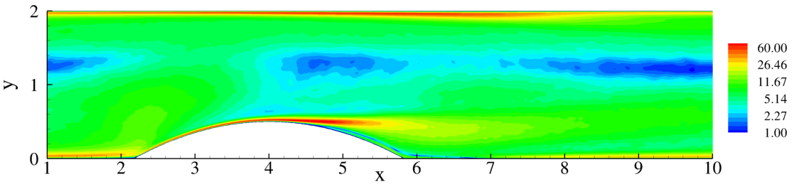
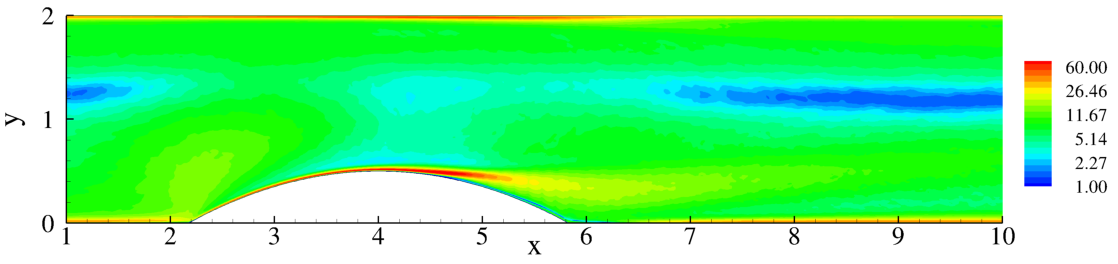
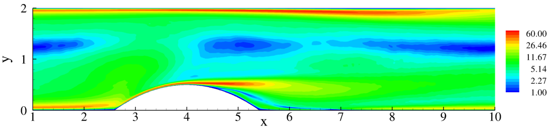
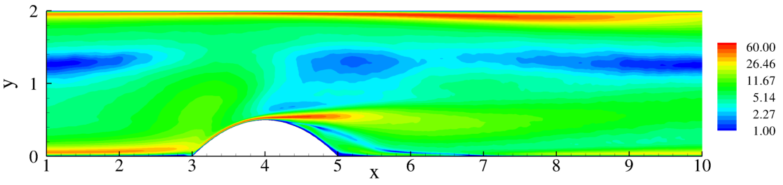
Figure 22: Shear intensity $S^{*}=S\,(2k_{T})/\epsilon_{T}=\left(L_{0}/L_{S}\right)^{2/3}$ in the flow domain for all simulations.

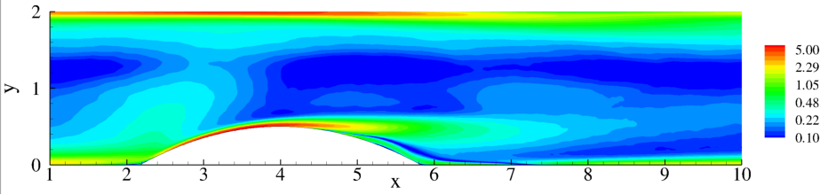
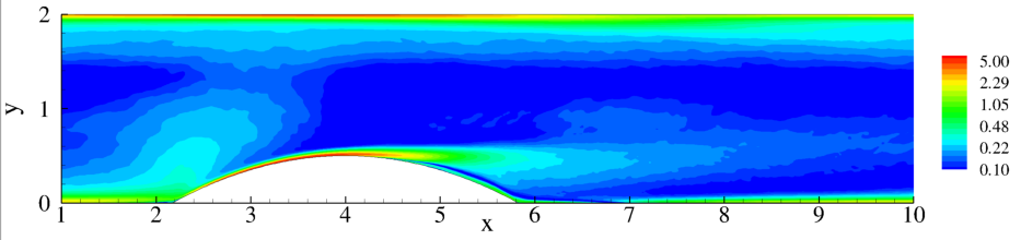
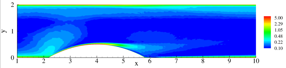
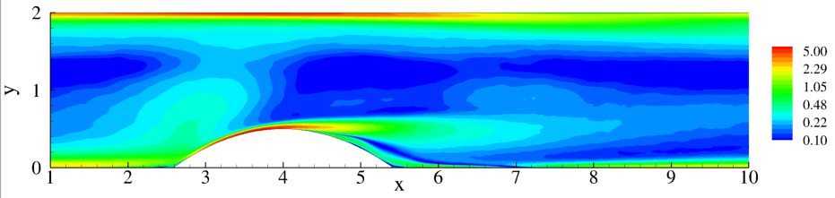
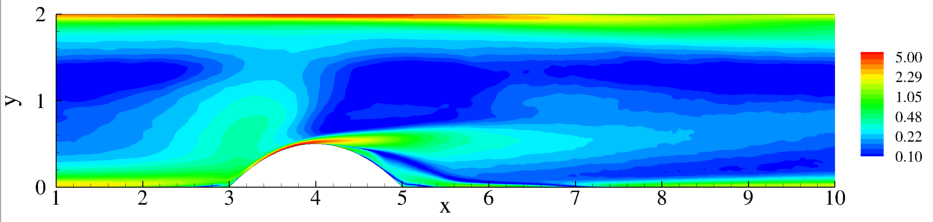
Figure 23: Corrsin parameter $S_{c}=S\sqrt{\nu/\epsilon_{T}}=\left(\eta/L_{S}\right)^{2/3}$ in the flow domain for all simulations.

3.4.4 Invariant Maps

The Anisotropy Invariant Map (AIM) originally introduced by Lumley & Newman (1977); Lumley (1979) provides a description of the different anisotropic states of the large turbulent scales. They are quantified in terms of the invariants of the anisotropy tensor, i.e. the deviatoric component of the Reynolds stress, $b_{ij}$, namely $I=b_{ii}=0$, $II=b_{ij}\,b_{ji}$ and $III=b_{ij}\,b_{jk}\,b_{ki}$. The admissible states of the flow must lie within a (curvilinear) triangle of the $II-III$ plane. This constraint comes from the requirement that the eigenvalues of $b_{ij}$ should be real and the squared velocity fluctuation in the principal direction must be positive. The admissible region is delimited above by the line $II=2/9+2III$ corresponding to statistically two-dimensional turbulence, i.e. the fluctuation intensity in one of the eigen-directions vanishes. The other two limiting lines, $II=3/2\left(16/9\,III^{2}\right)^{1/3}$, represent axisymmetric turbulence, i.e. the fluctuation intensity in two eigen-directions are identical. In the left branch ($III<0$), the fluctuation intensity in the third eigen-direction is smaller than the other two (pancake turbulence). In the right branch ($III>0$), the third component is larger than the other two (cigar-like turbulence). The corners correspond to: the isotropic state ($II=0,\,III=0$), the two-component isotropic state ($II=-1/36,\,III=1/6$), and the one-component state ($II=2/9,\,III=2/3$). In many applications, turbulence modelling exploits the idea of eddy viscosity which assumes that the Reynolds stress tensor is proportional (via the eddy-viscosity) to the mean strain rate tensor, see Speziale (1991); Gatski & Speziale (1993). Modelling is particularly challenging for separated flows. The AIM is helpful to directly take into account the anisotropy of the flow, see Jovičić et al. (2006); Kumar et al. (2009) and the general discussion in Jovanovic (2013) where $II$ and $III$ are used to compute the length scale appearing in the eddy-viscosity thus including anisotropic effects in the model.

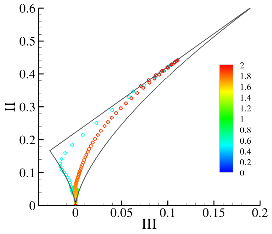
Figure 24: Anisotropy Invariant Map for case C1 at: (a) the tip of the bump; (b) end of the bump; (c) inside the recirculation region. Note that (a), (b) and (c) correspond to stations b), c) and d) of figure1. The color legend represents the $y$ coordinate.

Figure 24 shows the AIM for simulation C1 at three stations. At the tip of the bump, panel (a), close to the bump wall at $y=0.5$, turbulence is essentially two-dimensional. As $y$ increases, the points in the plot approach the lower left branch indicating axisymmetric turbulence. As expected, close to the centreline of the channel, the flow becomes isotropic. As the top wall is approached, the flow follows a trend similar to what is found in a planar channel (Gilbert & Kleiser, 1991) becoming two-dimensional again (red points) at the top wall. However, in our case due to the adverse pressure gradient at the top wall the trajectory followed in the map by the orange/red points is shifted away from the right branch, departing from the axisymmetric state typical of the planar channel flow. Panel (b) corresponds to the end of the bump which exhibits a more complex AIM. As the $y$ coordinate increases, the initial axisymmetric state is hardly reached and the trajectory in the $II-III$ plane follows an inner path towards the opposite axisymmetric state ($III>0$) as the shear layer is crossed (light blue). At the centreline, the flow is again isotropic and follows an inner path towards the top wall. These results are typical of separated flows as found, e.g., in the backward facing step configuration (Le et al., 1997b). Panel (c) shows the trajectory at a station closer to the reattachment point. Flow close to the lower wall is completely axisymmetric ($III<0$) until the shear layer is reached (light blue). The turbulence shifts from axisymmetric contraction to axisymmetric expansion, similar to panel (b). The flow is isotropic at the centreline and follows the same trend discussed for panel (a) and (b) as the top wall is reached. The analysis of the AIM suggests that the flow we are addressing is rather complex to model, due to the presence of the recirculating region behind the bump and the adverse pressure gradient along the top wall.

4 Conclusions

Turbulent separation behind a bump in channel flow is addressed using Direct Numerical Simulations (DNS) for different bump geometries and for Reynolds number ranging between $\Rey=2500$ and $\Rey=10000$. The latter is probably the largest Reynolds number ever achieved in the DNS of this specific configuration, corresponding to a maximum friction Reynolds number of approximately $\Rey_{\tau}=900$.

The separation behind the bump generates small scale structures which grow downstream, an intense shear layer and a recirculating region after the bump. Although the recirculation size depends on geometry, the reattachment position is constant. The reattachment point is controlled by the Reynolds number based on the bump height, as confirmed by the available experimental data, Kähler et al. (2016).

With increasing Reynolds number, a net decrease in drag coefficient is observed in association with the reduced dimensionless pressure drop needed to maintain the flow rate constant. The reduction is overwhelmed by the increase in the dimensional velocity, quadratically entering the expression for the drag force, leading to the expected increase in flow resistance. The drag increase with respect to that of an equivalent planar channel is almost entirely due to form effects induced by the separation, even though a significant increase in velocity, hence in local wall shear stress, is measured at the bump tip. At larger Reynolds number, the shear layer separating the recirculation bubble from the outer stream becomes more attached to the lower wall. Its fluctuations correspond to higher turbulent kinetic energy production peaks. The DNS captures a small recirculation originated by the sudden change in slope at the bump leading edge. The separation at the bottom wall affects the opposite near-wall region by inducing a significant adverse pressure gradient which is not sufficient to separate the flow at the upper wall.

Due to the strong non-homogeneity and the resulting mean gradients, the mean flow draws energy from the local external energy source, namely the pressure drop multiplied by velocity. The uptake mostly occurs in the bulk. Fluxes move this energy to the shear layer where it is partially dissipated but mostly intercepted by the production term to sustain the turbulent fluctuations. The dissipation in the mean flow is significant, given the strong mean gradients present at the walls and in the shear layer. Overall, the most important feature is the peak of turbulent kinetic energy production localised in the shear layer. The path taken by this energy bifurcates, in part sustaining the turbulent fluctuations inside the bubble and in part feeding the turbulence of the external flow downstream of the bubble. From the most streamlined to the bluffest bump, a 50% increase in peak energy production is observed. For fixed geometry, a fourfold Reynolds number change leads to approximately 400% increase in peak production.

In turbulence modelling, the level of anisotropy at both the large and small scales is crucial. They can be characterised in terms of the deviatoric components of Reynolds stress and pseudo-dissipation tensor, respectively. Apart from the near wall region, anisotropy at both large and small scales concentrates in the shear layer, irrespective of bump shape and Reynolds number. Interestingly, the small scales keep a high level of anisotropy in the shear layer, even at larger Reynolds number. This is due to the intensity of the mean gradients which maintain the production active close to dissipation scales. Finally, the analysis of the anisotropy invariant maps shows that the separated flow poses a significant difficulty for turbulence modelling due to the recirculating region behind the bump and the adverse pressure gradient along the top wall.

The research has received funding from the European Research Council under the ERC Grant Agreement no. 339446. We acknowledge PRACE for awarding us access to supercomputing resource FERMI based in Bologna, Italy through PRACE project no. 2014112647.

References

- Alam & Sandham (2000) Alam, M. & Sandham, N. D. 2000 Direct numerical simulation of ‘short’laminar separation bubbles with turbulent reattachment. Journal of Fluid Mechanics 403, 223–250.
- Antonia et al. (1994) Antonia, R.A., Djenidi, L. & Spalart, P.R. 1994 Anisotropy of the dissipation tensor in a turbulent boundary layer. Physics of Fluids 6 (7), 2475–2479.
- Bai et al. (2014) Bai, HL, Zhou, Y, Zhang, WG, Xu, SJ, Wang, Y & Antonia, RA 2014 Active control of a turbulent boundary layer based on local surface perturbation. Journal of Fluid Mechanics 750, 316.
- Breuer et al. (2009) Breuer, M., Peller, N., Rapp, Ch. & Manhart, M. 2009 Flow over periodic hills–numerical and experimental study in a wide range of reynolds numbers. Computers & Fluids 38 (2), 433–457.
- Casciola et al. (2003) Casciola, C. M., Gualtieri, P., Benzi, R. & Piva, R. 2003 Scale-by-scale budget and similarity laws for shear turbulence. Journal of Fluid Mechanics 476.
- Casciola et al. (2007) Casciola, C. M., Gualtieri, P., Jacob, B. & Piva, R. 2007 The residual anisotropy at small scales in high shear turbulence. Physics of Fluids 19 (10), 101704.
- Castro & Epik (1998) Castro, I. P. & Epik, E. 1998 Boundary layer development after a separated region. Journal of Fluid Mechanics 374, 91–116.
- Chen et al. (2006) Chen, J., Meneveau, C. & Katz, J. 2006 Scale interactions of turbulence subjected to a straining–relaxation–destraining cycle. Journal of Fluid Mechanics 562, 123–150.
- Chong et al. (1998) Chong, M. S., Soria, J., Perry, A. E., Chacin, J., Cantwell, B. J. & Na, Y. 1998 Turbulence structures of wall-bounded shear flows found using dns data. Journal of Fluid Mechanics 357, 225–247.
- Cimarelli et al. (2013) Cimarelli, A., De Angelis, E. & Casciola, C. M. 2013 Paths of energy in turbulent channel flows. Journal of Fluid Mechanics 715, 436–451.
- Corrsin (1958) Corrsin, Stanley 1958 Local isotropy in turbulent shear flow. National Advisory Committee for Aeronautics.
- Dengel & Fernholz (1990) Dengel, P. & Fernholz, H.H. 1990 An experimental investigation of an incompressible turbulent boundary layer in the vicinity of separation. Journal of Fluid Mechanics 212, 615–636.
- Diosady & Murman (2014) Diosady, L. T. & Murman, S. M. 2014 Dns of flows over periodic hills using a discontinuous galerkin spectral-element method. AIAA Paper 2784, 2014.
- Elsberry et al. (2000) Elsberry, K., Loeffler, J., Zhou, M.D. & Wygnanski, I. 2000 An experimental study of a boundary layer that is maintained on the verge of separation. Journal of Fluid Mechanics 423, 227–261.
- Epstein & Ross (1999) Epstein, F. H. & Ross, R. 1999 Atherosclerosis—an inflammatory disease. New England journal of medicine 340 (2), 115–126.
- Fischer et al. (2008) Fischer, Paul F, Lottes, James W & Kerkemeier, Stefan G 2008 nek5000 web page. Web page: http://nek5000. mcs. anl. gov .
- Fröhlich et al. (2005) Fröhlich, J., Mellen, C. P., Rodi, W., Temmerman, L. & Leschziner, M. A. 2005 Highly resolved large-eddy simulation of separated flow in a channel with streamwise periodic constrictions. Journal of Fluid Mechanics 526, 19–66.
- Gatski & Speziale (1993) Gatski, TB & Speziale, Charles G 1993 On explicit algebraic stress models for complex turbulent flows. Journal of fluid Mechanics 254, 59–78.
- Gilbert & Kleiser (1991) Gilbert, N & Kleiser, L 1991 Turbulence model testing with the aid of direct numerical simulation results. In 8th Symposium on Turbulent Shear Flows, Volume 2, , vol. 2, pp. 26–1.
- Gualtieri et al. (2007) Gualtieri, P., Casciola, C. M., Benzi, R. & Piva, R. 2007 Preservation of statistical properties in large-eddy simulation of shear turbulence. Journal of Fluid Mechanics 592, 471–494.
- Gualtieri & Meneveau (2010) Gualtieri, P. & Meneveau, C. 2010 Direct numerical simulations of turbulence subjected to a straining and destraining cycle. Physics of Fluids (1994-present) 22 (6), 065104.
- Harun et al. (2013) Harun, Z., Monty, J. P., Mathis, R. & Marusic, I. 2013 Pressure gradient effects on the large-scale structure of turbulent boundary layers. Journal of Fluid Mechanics 715, 477–498.
- Hickel et al. (2008) Hickel, S., Kempe, T. & Adams, N.A. 2008 Implicit large-eddy simulation applied to turbulent channel flow with periodic constrictions. Theoretical and Computational Fluid Dynamics 22 (3-4), 227–242.
- Jacob et al. (2008) Jacob, B., Casciola, C. M., Talamelli, A. & Alfredsson, P. H. 2008 Scaling of mixed structure functions in turbulent boundary layers. Physics of Fluids (1994-present) 20 (4), 045101.
- Jovanovic (2013) Jovanovic, Jovan 2013 The statistical dynamics of turbulence. Springer Science & Business Media.
- Jovičić et al. (2006) Jovičić, N, Breuer, M & Jovanović, J 2006 Anisotropy-invariant mapping of turbulence in a flow past an unswept airfoil at high angle of attack. Journal of fluids engineering 128 (3), 559–567.
- Kähler et al. (2016) Kähler, C. J., Scharnowski, S. & Cierpka, C. 2016 Highly resolved experimental results of the separated flow in a channel with streamwise periodic constrictions. Journal of Fluid Mechanics 796, 257–284.
- Kim et al. (1987) Kim, J., Moin, P. & Moser, R. 1987 Turbulence statistics in fully developed channel flow at low reynolds number. Journal of fluid mechanics 177, 133–166.
- Krogstad & Skaare (1995) Krogstad, P. A. & Skaare, P. E. 1995 Influence of the strong adverse pressure gradient on the turbulent structure in a boundary layer. Physics of Fluids 7 (8), 2014–2024.
- Kuban et al. (2012) Kuban, L., Laval, J.-P., Elsner, W., Tyliszczak, A. & Marquillie, M. 2012 Les modeling of converging-diverging turbulent channel flow. Journal of Turbulence (13), N11.
- Kumar et al. (2009) Kumar, V, Frohnapfel, B, Jovanović, J, Breuer, M, Zuo, Wangda, Hadzić, I & Lechner, R 2009 Anisotropy invariant reynolds stress model of turbulence (airsm) and its application to attached and separated wall-bounded flows. Flow, turbulence and combustion 83 (1), 81–103.
- Laval et al. (2012) Laval, J.-P., Marquillie, M. & Ehrenstein, U. 2012 On the relation between kinetic energy production in adverse-pressure gradient wall turbulence and streak instability. Journal of Turbulence (13), N21.
- Le et al. (1997a) Le, H., Moin, P. & Kim, J. 1997a Direct numerical simulation of turbulent flow over a backward-facing step. Journal of fluid mechanics 330, 349–374.
- Le et al. (1997b) Le, Hung, Moin, Parviz & Kim, John 1997b Direct numerical simulation of turbulent flow over a backward-facing step. Journal of fluid mechanics 330 (1), 349–374.
- Lee et al. (1990) Lee, Moon Joo, Kim, John & Moin, Parviz 1990 Structure of turbulence at high shear rate. Journal of Fluid Mechanics 216, 561–583.
- Lozano-Durán & Jiménez (2014) Lozano-Durán, A. & Jiménez, J. 2014 Effect of the computational domain on direct simulations of turbulent channels up to . Physics of Fluids 26 (1), 011702.
- Lumley (1979) Lumley, John L 1979 Computational modeling of turbulent flows. Advances in applied mechanics 18, 123–176.
- Lumley & Newman (1977) Lumley, John L & Newman, Gary R 1977 The return to isotropy of homogeneous turbulence. Journal of Fluid Mechanics 82 (01), 161–178.
- Marati et al. (2004) Marati, N., Casciola, C. M. & Piva, R. 2004 Energy cascade and spatial fluxes in wall turbulence. Journal of Fluid Mechanics .
- Marquillie et al. (2011) Marquillie, M., Ehrenstein, U. & Laval, J.-P. 2011 Instability of streaks in wall turbulence with adverse pressure gradient. Journal of Fluid Mechanics 681 (205-240), 30.
- Marquillie & Ehrenstein (2003) Marquillie, M. & Ehrenstein, U. W. E. 2003 On the onset of nonlinear oscillations in a separating boundary-layer flow. Journal of Fluid Mechanics 490, 169–188.
- Marquillie et al. (2008) Marquillie, M., Laval, J.-P. & Dolganov, R. 2008 Direct numerical simulation of a separated channel flow with a smooth profile. Journal of Turbulence (9), N1.
- Marusic et al. (2013) Marusic, I., Monty, J. P., Hultmark, M. & Smits, A. J. 2013 On the logarithmic region in wall turbulence. Journal of Fluid Mechanics 716, R3.
- Marusic et al. (2014) Marusic, I, Talluru, KM & Hutchins, N 2014 Controlling the large-scale motions in a turbulent boundary layer. In Fluid-Structure-Sound Interactions and Control, pp. 17–26. Springer.
- Mellen et al. (2000) Mellen, C. P., Frölich, J. & Rodi, W. 2000 Large eddy simulations of the flow over periodic hills. In IMACS World Congress.
- Na & Moin (1998a) Na, Y. & Moin, P. 1998a Direct numerical simulation of a separated turbulent boundary layer. Journal of Fluid Mechanics 374, 379–405.
- Na & Moin (1998b) Na, Y. & Moin, P. 1998b The structure of wall-pressure fluctuations in turbulent boundary layers with adverse pressure gradient and separation. Journal of Fluid Mechanics 377, 347–373.
- Nagib & Chauhan (2008) Nagib, H. M. & Chauhan, K. A. 2008 Variations of von kármán coefficient in canonical flows. Physics of Fluids 20 (10), 1518.
- Neumann & Wengle (2004) Neumann, J. & Wengle, H. 2004 Coherent structures in controlled separated flow over sharp-edged and rounded steps. Journal of Turbulence 5 (22), 14.
- Ohlsson et al. (2010) Ohlsson, J., Schlatter, P., Fischer, P. F. & Henningson, D. S. 2010 Direct numerical simulation of separated flow in a three-dimensional diffuser. Journal of Fluid Mechanics 650, 307–318.
- Patera (1984) Patera, A. T. 1984 A spectral element method for fluid dynamics. Journal of Computational Physics 54, 468–488.
- Peller & Manhart (2006) Peller, N. & Manhart, M. 2006 Turbulent channel flow with periodic hill constrictions. In New Results in Numerical and Experimental Fluid Mechanics V, pp. 504–512. Springer.
- Pumir et al. (2016) Pumir, Alain, Xu, Haitao & Siggia, Eric D 2016 Small-scale anisotropy in turbulent boundary layers. Journal of Fluid Mechanics 804, 5–23.
- Rapp & Manhart (2011) Rapp, Ch. & Manhart, M. 2011 Flow over periodic hills: an experimental study. Experiments in fluids 51 (1), 247–269.
- Robinson (1991) Robinson, S. K. 1991 Coherent motions in the turbulent boundary layer. Annual Review of Fluid Mechanics 23 (1), 601–639.
- Šarić et al. (2007) Šarić, S., Jakirlić, S., Breuer, M., Jaffrézic, B., Deng, G., Chikhaoui, O., Fröhlich, J., Von Terzi, D., Manhart, M. & Peller, N. 2007 Evaluation of detached eddy simulations for predicting the flow over periodic hills. In ESAIM: proceedings, , vol. 16, pp. 133–145. EDP Sciences.
- Simpson (1989) Simpson, R. L. 1989 Turbulent boundary-layer separation. Annual Review of Fluid Mechanics .
- Skaare & Krogstad (1994) Skaare, P. E. & Krogstad, P. A. 1994 A turbulent equilibrium boundary layer near separation. Journal of Fluid Mechanics 272, 319–348.
- Skote & Henningson (2002) Skote, M. & Henningson, D. S. 2002 Direct numerical simulation of a separated turbulent boundary layer. Journal of Fluid Mechanics 471, 107–136.
- Skote et al. (1998) Skote, M., Henningson, D. S. & Henkes, R. A. W. M. 1998 Direct numerical simulation of self-similar turbulent boundary layers in adverse pressure gradients. Flow, turbulence and combustion 60 (1), 47–85.
- Soria et al. (2017) Soria, J., Kitsios, V., Atkinson, C., Sillero, J. A., Borrell, G., Gungar, A. G. & Jimenez, J. 2017 Towards the direct numerical simulation of a self-similar adverse pressure gradient turbulent boundary layer flow. In Whither Turbulence and Big Data in the 21st Century?, pp. 61–75. Springer.
- Spalart (1988) Spalart, P. R. 1988 Direct simulation of a turbulent boundary layer up to r = 1410. Journal of Fluid Mechanics 187, 61–98.
- Spalart & Watmuff (1993) Spalart, P. R. & Watmuff, J. H. 1993 Experimental and numerical investigation of a turbulent boundary layer with pressure gradients. Journal of Fluid Mechanics 249, 337–371.
- Speziale (1991) Speziale, Charles G 1991 Analytical methods for the development of reynolds-stress closures in turbulence. Annual Review of Fluid Mechanics 23 (1), 107–157.
- Temmerman et al. (2003) Temmerman, L., Leschziner, M. A., Mellen, Christopher P. & Fröhlich, J. 2003 Investigation of wall-function approximations and subgrid-scale models in large eddy simulation of separated flow in a channel with streamwise periodic constrictions. International Journal of Heat and Fluid Flow 24 (2), 157–180.
- Van Dyke (1982) Van Dyke, M. 1982 An album of fluid motion .
- Webster et al. (1996) Webster, D. R., DeGraaff, D. B. & Eaton, J. K. 1996 Turbulence characteristics of a boundary layer over a two-dimensional bump. Journal of Fluid Mechanics 320, 53–69.
- Wilcox (1998) Wilcox, D. C. 1998 Turbulence modeling for CFD, , vol. 2. DCW industries La Canada, CA.
- Wu & Squires (1998) Wu, X. & Squires, K. D. 1998 Numerical investigation of the turbulent boundary layer over a bump. Journal of Fluid Mechanics 362, 229–271.