Orbits in the T Tauri triple system observed with SPHERE

Abstract

Aims. We present new astrometric measurements of the components in the T Tauri system, and derive new orbits and masses.

Methods. T Tauri was observed during the science verification time of the new extreme adaptive optics facility SPHERE at the VLT. We combine the new positions with recalibrated NACO-measurements and data from the literature. Model fits for the orbits of T Tau Sa and Sb around each other and around T Tau N yield orbital elements and individual masses of the stars Sa and Sb.

Results. Our new orbit for T Tau Sa/Sb is in good agreement with other recent results, which indicates that enough of the orbit has been observed for a reliable fit. The total mass of T Tau S is $2.65\pm 0.11\,M_{\odot}$. The mass ratio $M_{\rm Sb}:M_{\rm Sa}$ is $0.25\pm 0.03$, which yields individual masses of $M_{\rm Sa}=2.12\pm 0.10\,M_{\odot}$ and $M_{\rm Sb}=0.53\pm 0.06\,M_{\odot}$. If our current knowledge of the orbital motions is used to compute the position of the southern radio source in the T Tauri system, then we find no evidence for the proposed dramatic change in its path.

1 Introduction

T Tauri is a triple star which became the eponymous member of the class of low-mass, pre-main-sequence stars. It is located in the Taurus-Auriga star-forming region at a distance of $146.7\pm 0.6\rm\,pc$ (Loinard et al. 2007b). As brightest member of the class, it was the subject of many studies of the stellar components and/or the circumstellar material surrounding them.

Using speckle-interferometry, Dyck et al. (1982) were able to resolve T Tauri into two components separated by about $0\aas@@fstack{\prime\prime}7$, which are commonly called T Tau N and T Tau S. The southern component is only visible in the infrared, it has not been detected in the V-band down to 19.6 mag (Stapelfeldt et al. 1998). With the construction of larger telescopes, it became possible to resolve T Tau S itself into two stars named T Tau Sa and T Tau Sb (Koresko 2000). Because of their small separation ($\sim\,$50 mas at the time of the discovery) and short orbital period, it is possible to determine their orbital parameters within a reasonable time span. A number of authors have presented orbit fits (e.g. Beck et al. 2004; Johnston et al. 2004; Duchêne et al. 2006; Schaefer et al. 2006; Köhler et al. 2008; Köhler 2008; Schaefer et al. 2014), where the precision of the orbital parameters improved as more observational data became available. The nearby third component T Tau N can be used as astrometric reference to determine the individual orbits of Sa and Sb around their center of mass (Duchêne et al. 2006; Köhler et al. 2008; Köhler 2008). The ratio of the semi-major axes is equal to their mass ratio, while the sum of both masses can be computed from the Sa/Sb orbit. Together, we obtain individual masses for Sa and Sb. It turned out that T Tau Sa is the most massive component in the triple system, despite its faintness at optical and near-IR wavelengths (it was never detected in J-band, including the new SPHERE observations). The currently most likely explanation for this is that T Tau Sa and Sb are hidden behind circumstellar and/or circumbinary material (Duchêne et al. 2005).

In this work, we report on our astrometric analysis of observations taken during the science verification time of SPHERE. The data was analyzed independently by a different team, who presented their results in Csépány et al. (2015). In addition to the SPHERE data, we also recalibrated all the available NACO-data, in order to provide a more consistent astrometric reference frame. This includes two NACO-observations that were not published before. We use these data to derive improved orbital elements and masses, and discuss the implications for our understanding of the system.

This paper reports on the astrometric measurements taken with SPHERE. The science verification data also allowed us to image the extended emission in the T Tauri system in unprecedented detail. These results will be presented in a subsequent paper (Kasper et al., submitted to A&A).

Table 1: Pixel Scale and Orientation of our NACO-observations.

Epoch	Pixel scale	P.A. of the $y$-axis
	[mas/pixel]	[∘]
Dec. 2001	$13.241\pm 0.011$	$1.26\pm 0.10$
Dec. 2002	$13.239\pm 0.028$	$0.01\pm 0.06$
Dec. 2003	$13.262\pm 0.025$	$0.18\pm 0.13$
Dec. 2004	$13.295\pm 0.024$	$0.01\pm 0.10$
Dec. 2006	$13.258\pm 0.020$	$0.50\pm 0.06$
Sep. 2007	$13.270\pm 0.010$	$0.43\pm 0.12$
Feb. 2008	$13.283\pm 0.004$	$0.47\pm 0.10$
Oct. 2008	$13.269\pm 0.015$	$0.54\pm 0.10$
Feb. 2009	$13.266\pm 0.013$	$0.54\pm 0.08$

Table 2: New and recalibrated astrometric measurements of T Tau N – Sa – Sb

Date (UT)

Epoch

T Tau N - Sa

T Tau Sa - Sb

Filter

Instrument

$d$ [mas]

P.A. $[^{\circ}]$

$d$ [mas]

P.A. $[^{\circ}]$

2001 Dec 08, 3:34

2001.93470

$693.70$${}\pm{}$

$0.66$

$181.88$${}\pm{}$

$0.11$

$99.60$${}\pm{}$

$0.80$

$276.80$${}\pm{}$

$0.40$

K

NACO

2002 Dec 15, 2:31

2002.95306

$694.21$${}\pm{}$

$1.57$

$182.56$${}\pm{}$

$0.10$

$106.50$${}\pm{}$

$1.60$

$284.10$${}\pm{}$

$0.20$

Ks

NACO

2003 Dec 12, 3:14

2003.94424

$692.93$${}\pm{}$

$2.18$

$183.07$${}\pm{}$

$0.13$

$112.70$${}\pm{}$

$0.80$

$288.70$${}\pm{}$

$0.80$

Ks

NACO

2004 Dec 09, 4:06

2004.93818

$697.89$${}\pm{}$

$1.64$

$183.74$${}\pm{}$

$0.14$

$119.70$${}\pm{}$

$1.20$

$296.10$${}\pm{}$

$0.60$

Ks

NACO

2006 Oct 11, 8:50

2006.77582

$694.75$${}\pm{}$

$1.38$

$185.21$${}\pm{}$

$0.07$

$125.10$${}\pm{}$

$0.80$

$304.99$${}\pm{}$

$0.20$

Ks

NACO

2007 Sep 16, 8:00

2007.70659

$694.41$${}\pm{}$

$0.92$

$185.59$${}\pm{}$

$0.13$

$127.20$${}\pm{}$

$0.60$

$308.80$${}\pm{}$

$0.40$

Ks

NACO

2008 Feb 01, 0:38

2008.08358

$695.10$${}\pm{}$

$0.24$

$185.95$${}\pm{}$

$0.10$

$127.10$${}\pm{}$

$0.20$

$310.85$${}\pm{}$

$0.14$

Ks

NACO

2008 Oct 17, 6:18

2008.79333

$695.00$${}\pm{}$

$1.66$

$186.36$${}\pm{}$

$0.10$

$129.30$${}\pm{}$

$1.30$

$314.50$${}\pm{}$

$0.70$

Ks

NACO

2009 Feb 18, 0:32

2009.13216

$690.84$${}\pm{}$

$2.32$

$186.94$${}\pm{}$

$0.13$

$124.60$${}\pm{}$

$1.20$

$315.11$${}\pm{}$

$0.60$

Ks

NACO

2014 Dec 09, 3:36

2014.93676

$689.98$${}\pm{}$

$0.64$

$191.53$${}\pm{}$

$0.10$

$110.33$${}\pm{}$

$0.25$

$345.40$${}\pm{}$

$0.15$

BrG

SPHERE

2015 Jan 23, 2:20

2015.05981

—

—

$109.27$${}\pm{}$

$0.44$

$345.70$${}\pm{}$

$0.25$

Ks

SPHEREa

• T Tau N hidden behind the coronographic mask.

2 Observations and data reduction

Many measurements of the relative positions of two or three of the components of T Tau have been published in the past (Ghez et al. 1995; Roddier et al. 2000; White & Ghez 2001; Koresko 2000; Köhler et al. 2000; Duchêne et al. 2002; Furlan et al. 2003; Beck et al. 2004; Duchêne et al. 2005, 2006; Schaefer et al. 2006; Köhler et al. 2008; Köhler 2008; Schaefer et al. 2014). We use all of these data to solve for the orbit, with the exception of the points by Mayama et al. (2006), because they deviate significantly from the model and the other measurements.

2.1 NACO

Between 2001 and 2009, T Tauri was observed almost yearly with the adaptive optics, near-infrared camera NACO at the ESO Very Large Telescope (VLT) on Cerro Paranal, Chile (Rousset et al. 2003; Lenzen et al. 2003). Most of the data have already been published (Köhler et al. 2008; Köhler 2008), with the exception of the observations in October 2008 and February 2009. However, the astrometric calibration of the published data was derived from a field near the Trapezium in the Orion Nebula Cluster and coordinates by McCaughrean & Stauffer (1994). By now, much better coordinates are available (Close et al. 2012). Therefore, we recalibrated all the available NACO-data of T Tauri. The results of the new calibration are listed in Table 1, the new relative positions of T Tauri in Table 2. The new calibration resulted on average in a pixel scale that is 0.2 % larger and a rotation by 0.3° compared to the old calibration.

2.2 SPHERE

T Tauri was observed during the science verification time of the extreme adaptive optics facility SPHERE (Spectro-Polarimetric High-contrast Exoplanet REsearch) at the VLT (Beuzit et al. 2008) on December 9, 2014 and January 23, 2015. It was the target of two different science programs (PIs: Markus Kasper and Gergely Csépány).

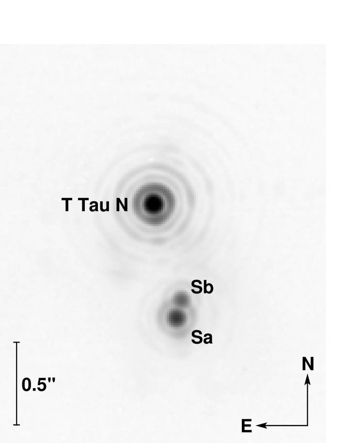
Figure 1: The T Tauri system imaged with SPHERE on December 9, 2014, displayed with a logarithmic scale.

We applied standard methods for infrared data reduction (dark subtraction, flatfield, and correction of bad pixels). Figure 1 shows one of the reduced images. The positions of the stars were measured with the Starfinder software (Diolaiti et al. 2000). Uncertainties were estimated by computing the standard deviation of positions measured in individual images.

In December 2014, T Tauri was imaged with the infrared dual-band imager and spectrograph (IRDIS) through a number of narrow-band filters. We measured the relative positions of the three components of T Tauri in the images obtained with the BrG filter, which has a central wavelength of $2162.9\rm\,nm$. The astrometric calibration was carried out by the instrument team and is described in the SPHERE user manual. During the science verification campaign, SPHERE observed a dedicated field in the outer region of the globular cluster 47 Tuc to derive astrometric calibration of the IRDIS broad-band H image, using the Hubble Space Telescope (HST) data as a reference (see Bellini et al. (2014) for the methods used to obtain HST measurements). The derived plate-scale was $12.232\pm 0.005\rm\,mas/pixel$ (for observations without a coronograph), and the $y$-axis of the IRDIS detector was at a position angle (P.A.) of $-1.764\pm 0.01^{\circ}$. The anamorphic distortion was corrected by multiplying the y-coordinates by $1.0062$. We used images taken with SPHERE’s internal grid mask to confirm that the pixel scale is the same with the H-band and the BrG filters.

In January 2015, images were recorded with IRDIS through a K-band filter. For most of these observations, T Tau N was hidden behind a coronographic mask (Csépány et al. 2015). Therefore, we did not measure its position, but only the relative positions of T Tau Sa and Sb. The pixel scale and orientation provided by the SPHERE consortium were used for the astrometric calibration.

The results for both observations are presented in Table 2. These data sets were reduced independently by Csépány et al. (2015), with different results for the positions. At the time of their analysis, the precise pixel scale and true north orientation were not known, which explains the different positions (G. Csépány, priv. comm.).

3 Orbit determination

3.1 The orbit of T Tauri Sa/Sb

To determine the orbit of T Tau Sa and Sb around each other, we followed the method described in Köhler et al. (2008). The first step was to find the best period, eccentricity and time of periastron with a grid search, while the remaining four orbital elements were written in the form of the Thiele-Innes constants and found using singular value decomposition. In a second step, we improved the results of this grid search by fitting all seven parameters simultaneously with a Levenberg-Marquardt $\chi^{2}$ minimization algorithm (Press et al. 1992). The orbit with the global minimum $\chi^{2}$ is shown in Fig. 2, and its orbital elements are listed in Table 3.

Table 3: Parameters of the best orbital solution for Sa – Sb.

Orbital Element	Value
Date of periastron $T_{0}$	$2450131$	$\,{}^{+208}_{-288}$
	(1996 Feb 17)
Period $P$ (years)	$27$	$\,{}^{+2}_{-2}$
Semi-major axis $a$ (mas)	$85$	$\,{}^{+4}_{-2}$
Semi-major axis $a$ (AU)	$12.5$	$\,{}^{+0.6}_{-0.3}$
Eccentricity $e$	$0.56$	$\,{}^{+0.07}_{-0.09}$
Argument of periastron $\omega$ (∘)	$48$	$\,{}^{+34}_{-25}$
P.A. of ascending node $\Omega$ (∘)	$92$	$\,{}^{+26}_{-36}$
Inclination $i$ (∘)	$20$	$\,{}^{+10}_{-6}$
System mass $M_{\rm S}$ ($\rm mas^{3}/year^{2}$)	$838$	$\,{}^{+29}_{-32}$
Mass error from distance error ($M_{\odot}$)		$\pm 0.032$
System mass $M_{\rm S}$ ($M_{\odot}$)	$2.65$	$\,{}^{+0.10}_{-0.11}$
reduced $\chi^{2}$	$2.7$
Mass ratio $M_{\rm Sb}/M_{\rm Sa}$	$0.25$	$\,\pm 0.03$
Mass of Sa $M_{\rm Sa}$ ($M_{\odot}$)	$2.12$	$\,\pm 0.10$
Mass of Sb $M_{\rm Sb}$ ($M_{\odot}$)	$0.53$	$\,\pm 0.06$

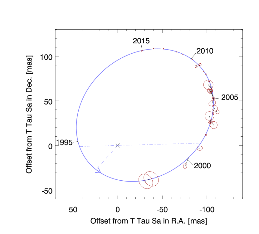
Figure 2: Best fitting orbit of T Tau Sb around Sa, in the rest frame of Sa. The observed positions are marked by their error ellipses and lines connecting the observed and calculated position at the time of the observations. The dash-dotted line indicates the line of nodes, the dashed line the periastron, and the arrow shows the direction of the orbital motion.

Uncertainties of the orbital elements were determined by analysing the $\chi^{2}$ function around its minimum. The 68 % confidence region for each parameter (the familiar $1\sigma$-interval in the case of a normal distribution) is the region where $\chi^{2}<\chi^{2}_{\rm min}+1$. Therefore, the uncertainties for the fit parameters depend on the value of $\chi^{2}$ at and around the minimum. The reduced $\chi^{2}$ of our fit was 2.7, more than one would expect for a good fit. This indicated that some of the measurement errors might have been underestimated. To avoid underestimating the uncertainties of the orbital elements as well, we rescaled the uncertainties of the observations so that the minimum $\chi^{2}$ was 1. Although some of the observations showed larger deviations from the model than others, we had no reason to trust any of the measurements less than the others. Therefore, we multiplied all observational uncertainties by the same factor $\sqrt{2.7}=1.64$. The uncertainties of the orbital elements in Table 3 are based on $\chi^{2}$ computed with these scaled measurement uncertainties.

Estimating the uncertainty of the mass required a special procedure. The mass itself was computed using Kepler’s third law ($M=a^{3}/P^{2}$, Kepler 1619). The semi-major axis $a$ and the period $P$ are usually strongly correlated. To obtain a realistic estimate for the uncertainty of the mass, we did not use standard error propagation. Instead, we considered a set of orbital elements where the semi-major axis was replaced by the mass. This is possible because Kepler’s third law gives an unambiguous relation between the two sets of elements. With the mass being one of the orbital elements, we treated it as one of the independent fit parameters and determined its uncertainty in the same way as for the other parameters.

3.2 The orbit of T Tauri S and the mass ratio $M_{\rm Sb}/M_{\rm Sa}$

The orbit of T Tau Sa and Sb around each other allows us to determine the sum of the masses of both components. To measure individual masses, we need to know the position of the center of mass (CM) of Sa and Sb. We followed the method described in Köhler et al. (2008) to do this. The path of the CM of Sa and Sb can be described in two ways: It is in orbit around T Tau N, and it is on the line from Sa to Sb, where its distance from Sa is a constant fraction of the separation of Sa and Sb. The fraction is $f=q/(1+q)$, with the mass ratio $q=M_{\rm Sb}/M_{\rm Sa}$.

Our model solves for eight parameters: the seven orbital elements of the orbit of the CM around T Tau N, and the fraction $f$. We compute $\chi^{2}$ from the difference between the position on the orbit and the position of the CM computed from the observed positions of Sa and Sb (note that the latter depends on the free parameter $f$). The fitting procedure is similar to that used for the orbit of Sa/Sb, except that the grid-search is carried out in 4 dimensions: eccentricity $e$, period $P$, time of periastron $T_{0}$, and the fractional mass $f$. Singular value decomposition was used again to fit the Thiele-Innes constants and hence the remaining orbital elements. To improve the fit further, about 150 orbit models with $\chi^{2}$ near the minimum were selected as starting points for a Levenberg-Marquart fit. Since this method assumes that the measurement errors are independent of the fitting parameters, $f$ cannot be treated like the other parameters. Instead, we perform a grid search over a narrow range in $f$ to find the minimum.

Köhler et al. (2008) and Köhler (2008) included unresolved observations of T Tau S as approximation for the position of the center of mass. However, the unknown offset between the center of light and the center of mass introduces an additional systematic error. Therefore, we used only resolved measurements of the positions of T Tau Sa and Sb in this work. Since both Köhler (2008) and this work are based on about 18 years of observational data, we can expect a fit of comparable quality.

If only the astrometric data were used, the best orbit solution corresponds to a system mass of 111$\,M_{\odot}$, which is clearly unphysical. In the same way as in Köhler et al. (2008), we introduced a system mass of $4.7\pm 1.0\,M_{\odot}$ as an additional constraint for the computation of $\chi^{2}$:

$$\chi^{2}=\sum_{i}\left(\@vec{r}_{i,\rm model}-\@vec{r}_{i,\rm obs}\over\Delta\@vec{r}_{i,\rm obs}\right)^{2}+\left(M_{\rm model}-4.7\,M_{\odot}\over 1.0\,M_{\odot}\right)^{2}$$

Here $\@vec{r}_{i,\rm obs}$ and $\Delta\@vec{r}_{i,\rm obs}$ are the observed position at time $i$ and the corresponding error, $\@vec{r}_{i,\rm model}$ is the position at time $i$ computed from the model, and $M_{\rm model}$ is the system mass computed from the orbit model. The mass estimate of $4.7\,M_{\odot}$ is the sum of our result for $M_{\rm S}$ in Sect. 3.1 and the mass of T Tau N estimated from its spectral energy distribution by Loinard et al. (2007b). They derived a mass for T Tau N of $1.83^{+0.20}_{-0.16}$ or $2.14^{+0.11}_{-0.10}$, depending on the theoretical pre-main-sequence track used. The uncertainty of $\pm 1.0\,M_{\odot}$ for our mass estimate was chosen to be about three times as large as the uncertainties of the estimates for $M_{\rm S}$ and $M_{\rm N}$, in order to avoid adding a constraint to the orbit fit that is more stringent than the astrometric data.

Table 4: Parameters of the best orbital solution for T Tau N–S.

Orbital Element	Value
Date of periastron $T_{0}$ (Epoch)	$1967$	$\,{}^{+25}_{-47}$
Period $P$ (years)	$4200$	$\,{}^{+5000}_{-3400}$
Semi-major axis $a$ (arcsec)	$2.9$	$\,{}^{+5.4}_{-1.7}$
Semi-major axis $a$ (AU)	$430$	$\,{}^{+790}_{-250}$
Eccentricity $e$	$0.7$	$\,{}^{+0.2}_{-0.4}$
Argument of periastron $\omega$ (∘)	$12$	$\,{}^{+10}_{-6}$
P.A. of ascending node $\Omega$ (∘)	$156$	$\,{}^{+11}_{-11}$
Inclination $i$ (∘)	$52$	$\,{}^{+4}_{-5}$
System mass ($\rm mas^{3}/year^{2}$)	$1468$	$\,{}^{+15}_{-15}$
Mass error from distance error ($M_{\odot}$)		$\pm 0.057$
System mass ($M_{\odot}$)	$4.6$	$\,{}^{+0.1}_{-0.1}$
reduced $\chi^{2}$	$3.7$

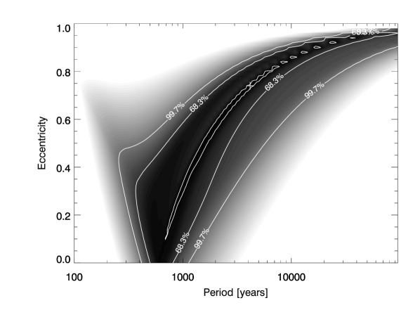
Figure 3: $\chi^{2}$ as function of period and eccentricity for the orbit of T Tau S around T Tau N. The cross marks the location of the best-fitting orbit solution (see Table 4). Contour lines show the $68.3\,\%$ and $99.7\,\%$ confidence regions (equivalent to $1\sigma$ and $3\sigma$ for a normal distribution). The innermost contour line is at $\chi^{2}_{\rm min}+0.2$. This has no particular significance, but demonstrates how flat $\chi^{2}$ is around the minimum.

The model with minimum $\chi^{2}$ is presented in Table 4, while the mass ratio $M_{\rm Sb}/M_{\rm Sa}$ is given in Table 3. Uncertainties were determined in the same way as for the orbit of Sa/Sb, Table 4 gives the 68 % confidence intervals. The uncertainties for the orbital elements are still large, due to the short section covered by the observations. Figure 3 shows $\chi^{2}$ of our orbit models as function of period and eccentricity. The orbit model whose parameters are listed in Table 4 is only one out of a wide range of models that fit the data almost equally well. Figure 4 shows the (formally) best orbit, the orbits at the lower and upper end of the 68 % confidence interval for the orbital period, and one circular orbit (eccentricity $e=0$). In the part of the orbit where observations have been collected, they are indistinguishable.

However, the main purpose of the fit is to determine the mass ratio of Sa and Sb, which is well constrained. Figure 5 shows the mass ratio as function of the orbital period for 150 orbit models that were the result of Levenberg-Marquart fits. Despite the large range in period, the mass ratio of all these solutions are remarkable similar. Even though the orbit of T Tau S around N is only weakly constrained, we are confident that our mass ratio $M_{\rm Sb}/M_{\rm Sa}$ is accurate within the uncertainties.

Figure 6 shows the motion of T Tau Sa and Sb in the rest frame of T Tau N, while Fig. 7 shows the offset of T Tau Sb as function of time. Both figures demonstrate that our model is a good fit for the motion of Sa and Sb relative to T Tau N.

The high eccentricity of the best-fitting orbit is surprising. However, high-eccentricity orbits are often the result of orbit fits to data that cover only a small fraction of the orbit. As more data are collected, the orbit solution usually converges towards an orbit with much lower eccentricity. We expect that this is also the case for the orbit of T Tau N/S. Therefore, the orbit presented in Table 4 should not be regarded as the most likely orbit, but only as one example of a large family of possible solutions. Even the confidence intervals in Table 4, while formally correct, are only an approximate representation to the probability distribution of the parameters. Even a circular orbit can not be ruled out from the data available (see Fig. 4).

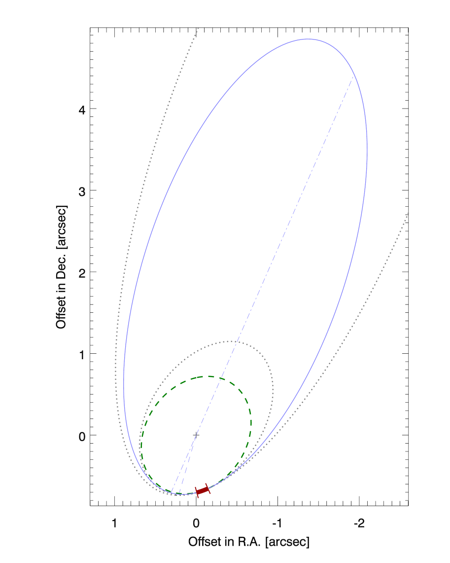
Figure 4: Motion of T Tau S around T Tau N. The solid line shows the orbit with the minimum $\chi^{2}$. The dotted lines show orbits at the short and long end of the confidence interval for the period (see Table 4), while the best circular orbit is shown by the dashed line. The thick section marks the part of the orbit that has been observed so far.

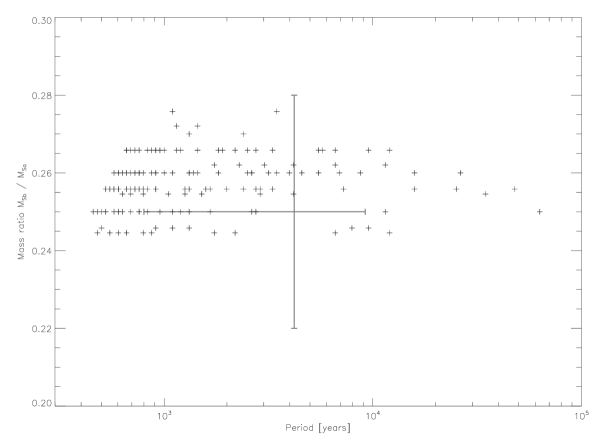
Figure 5: Mass ratio $M_{\rm Sb}/M_{\rm Sa}$ as function of the period of the T Tau N-S orbit model. These are the results of 150 runs of a Levenberg-Marquart fit starting with different initial estimates for the parameters (see Sect. 3.2). The quantized appearance is caused by the grid-based fit method for the mass ratio. The large cross indicates the 68 % confidence intervals for the period and mass ratio (see Tables 3 and 4). Note that the models plotted encompass a larger range in period than the 68 % confidence interval of the best solution.

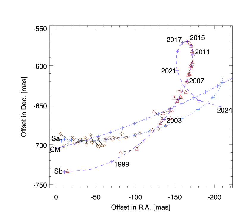
Figure 6: Motion of T Tau Sa and Sb in the reference frame of T Tau N. The path of Sa predicted by our orbit models is shown by the dotted line, the path of Sb by the dashed line, and the path of their center of mass by the dash-dotted line. The predicted positions on January 1 in every other year between 1997 and 2024 are marked by crosses. The observed positions of Sa are depicted by diamonds, those of Sb by triangles. Solid lines connect the observed and the predicted positions.

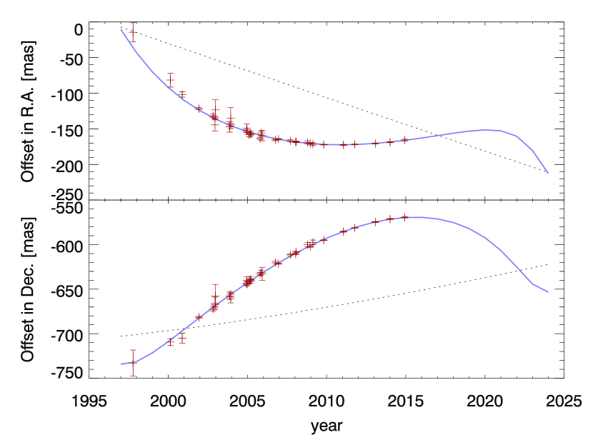
Figure 7: Offsets of T Tau Sb from T Tau N. The observed positions are marked by crosses with error bars. The solid line is our best fit for the motion of T Tau Sb, while the dotted line shows the motion of the center of mass of T Tau Sa and Sb.

Given the large uncertainty about the orbit, it might be surprising that the uncertainty of the system mass is very small, significantly smaller than in the term we added in the computation of $\chi^{2}$. However, to determine the mass, it is not always necessary to know the full orbit (see Sect. 4.2 in Köhler et al. 2008). The mass can be computed if both separation and acceleration are known. This is usually not the case for astrometric orbits, since their component parallel to the line of sight cannot be measured. However, these components are zero if the companion is at one of the nodes of the orbit. The information about separation and acceleration is inherently present in the data and results in an orbit solution with a well-constrained mass.

In the case of the orbit of T Tau N and S, the mass constraint selected one family of orbits from the larger set of orbits that agree with the astrometric data. For this family of orbits, the line of nodes is sufficiently close to the observations to result in a small mass uncertainty.

4 Discussion

4.1 Comparison to previous results

The orbital elements for our best fit for the motion of T Tau Sa and Sb around each other are very similar to the preliminary orbit presented by Schaefer et al. (2014). Both solutions agree well within $1\sigma$. We take this as sign that the fraction of the orbit observed so far is large enough to allow a reliable orbit fit, and that our orbits are close to the true orbit.

Most of the uncertainties of our orbit are significantly smaller than for the orbit of Schaefer et al. (2014). Although more and better data should improve the fit, we did not expect to reduce some of the uncertainties by a factor of two, since the orbital coverage was only extended by one year. This might be due to the improved calibration of the old NACO data. However, the argument of periastron and the P. A. of the line of nodes of our solution are less well constrained than those of Schaefer et al. (2014). The position of the periastron is difficult to determine, since the inclination of the orbit counteracts the (already moderate) eccentricity of the orbit, resulting in a projected orbit that is closer to circular than the true orbit. The small inclination of only $20^{\circ}$ (smaller than in Schaefer et al. (2014)) makes it more difficult to find the orientation of the line of nodes. Finally, the P. A. of the line of nodes and the argument of periastron are correlated, since only both angles together give the position of the periastron relative to north.

We note that a similar orbit was already published in Köhler (2008), which was significantly different from the orbit in Köhler et al. (2008), although only one additional astrometric measurement was used in Köhler (2008).

For the orbit of T Tau N and S around each other, the observed section is very small (less than 10° in position angle), which results in very large errors for any orbital elements derived from the data. It would be premature to even speak of a “preliminary orbit”. Given the large uncertainties, it is also not possible to predict when a reasonable solution will be possible. Nevertheless, our orbit solution is similar to the orbits presented in Köhler (2008) and Csépány et al. (2015). The period and semi-major axis are better constrained, due to the new data acquired since Köhler (2008) and the better calibration compared to Csépány et al. (2015).

However, to estimate the mass ratio $M_{\rm Sb}/M_{\rm Sa}$, we do not need the full orbit of T Tau S around N, but only a good estimate of the path of the center of mass at the times of our observations. Therefore, we can derive the mass ratio with relatively small uncertainties. In fact, our value of $0.25\pm 0.03$ is close to those reported by Duchêne et al. (2006) and Köhler (2008). Inclusion of the new data reduced the uncertainty of the mass ratio and the masses of Sa and Sb by a factor 2 – 3.

4.2 The compact radio source near T Tau Sb

Loinard et al. (2003, 2005) observed a compact radio source which they identified with T Tau Sb. Their astrometric measurements indicate a dramatic change in the motion of the radio source. Loinard et al. (2003) speculated that T Tau Sb underwent an ejection and might even leave the system on an unbound orbit. However, Furlan et al. (2003) found that T Tau Sb and the radio source move on distinct paths, and suggested a fourth object as the source of the radio emission.

In our orbit fit described in Sect. 3.1, we also tried parabolic and hyperbolic orbits for T Tau Sb, i.e. unbound orbits that would result in T Tau Sb leaving the system. These orbits do not fit the data very well, the best orbit has a reduced $\chi^{2}=5.82$, much higher than the best elliptical (bound) orbit. Furthermore, if T Tau Sb was on one of the unbound orbits matching the data, it would leave the system in an eastern direction. This is almost the opposite direction of the motion of the radio source (cf. Loinard et al. 2003).

In Fig. 8, we compare the positions of the radio source reported by Loinard et al. (2003) and our orbit of T Tau Sb, both in the reference frame of the center of mass of T Tau Sa+Sb. Note that the radio positions in this plot differ from those in Loinard et al. (2003). Loinard et al. (2003) computed the offsets from T Tau Sa with a linear approximation of the path of Sa, which does not take into account the orbital motion of Sa and Sb. We recalculated the offsets of the radio source from T Tau N, and subtracted the position of the CM of Sa+Sb, computed from the orbit found in Sect. 3.2. With the recalculated offsets, there is hardly any sign of a dramatic change of its orbit.

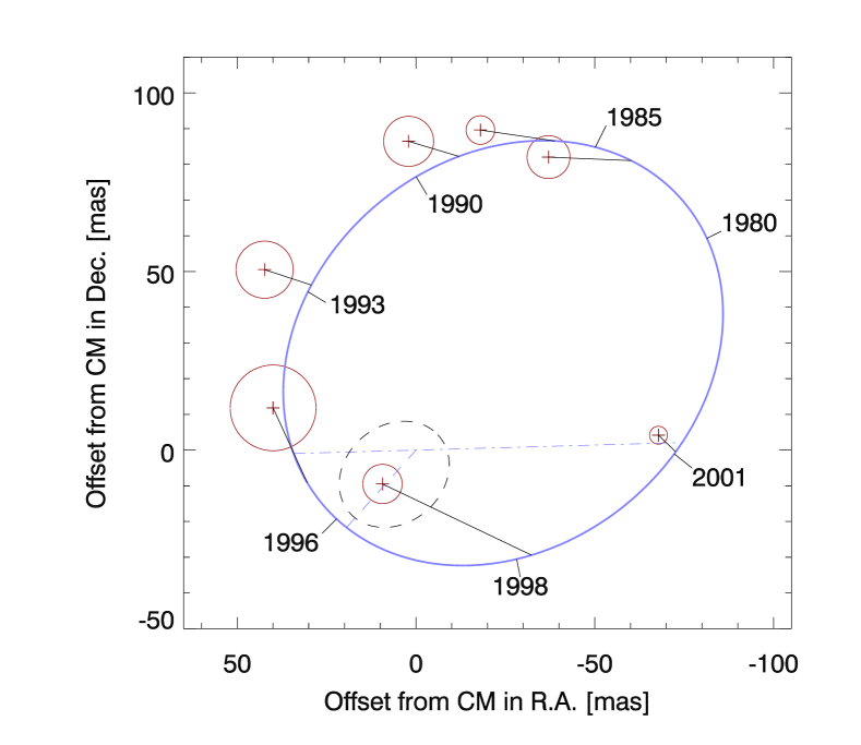
Figure 8: Positions of the radio source reported by Loinard et al. (2003), in the reference frame of the center of mass of T Tau Sa+Sb. Overplotted are our orbits for T Tau Sa (dashed ellipse) and T Tau Sb (continuous ellipse). Lines connect the positions of the radio source with the expected position of T Tau Sb at the same time.

However, it is obvious that the radio source is not identical with T Tau Sb. Yet they appear to be close enough to imply a relation between the star and the radio source. Loinard et al. (2007a) suggested the radio emission comes from the jets of Sb hitting the circumbinary disk. If this is true, then it is surprising that the position of the radio source relative to T Tau Sb changes within a few years. However, our knowledge of the geometry of the system is limited. Ratzka et al. (2009) argue that the circumstellar disk around T Tau Sb is seen not far from face-on, which implies that the jet axis is close to the line of sight. The circumbinary disk has to be nearly edge-on to provide the observed extinction. This means that the circumbinary disk is not aligned with the disk around T Tau Sb or the binary orbit. Given this complex geometry, it is conceivable that the offset from T Tau Sb of the intersection of jet and circumbinary disk changes on the timescale of the binary orbit.

There appears to be a systematic offset between T Tau Sb and the radio source, with the radio source always east of the star. This might indicate the orientation of the jet. However, considering the difficulties in registering the radio observations with the infrared images and the uncertainties of the T Tau N-S orbit which was extrapolated more than 20 years into the past, estimating the jet direction from this systematic offset would be extremely uncertain.

Finally, we note that the circumbinary material in front of T Tau S has to be distributed over at least 20 – 25 AU in both R.A. and Dec. to explain the permanently high extinction of T Tau Sb. The star has been observed from the most southern to the most northern point in its orbit, but no significant brightening was observed. The material causing the extinction might not be circumbinary, but a cloud in the T Tau system that happens to lie on our line of sight to T Tau S.

4.3 Are there more components in the system?

Nisenson et al. (1985) detected another source $0\aas@@fstack{\prime\prime}27$ north of T Tau N using speckle imaging techniques in the visual wavelength regime. The source was later identified in the K-band by Maihara & Kataza (1991), but neither Gorham et al. (1992) nor Stapelfeldt et al. (1998) detected it. The magnitude difference to T Tau N was $4.33\pm 0.09\rm\,mag$ at 521 nm (Nisenson et al. 1985) and $3.46\pm 0.32\rm\,mag$ in the K-band (Maihara & Kataza 1991).

Csépány et al. (2015) found a tentative companion 144 mas south of T Tau N. They found magnitude differences of $4.96\pm 0.30\rm\,mag$ at $1.02\rm\,\mu m$ and $4.37\pm 0.30\rm\,mag$ at $1.34\rm\,\mu m$. Considering the long time difference and the different wavelengths, this is comparable to the brightness reported by Nisenson et al. (1985) and Maihara & Kataza (1991).

If both Nisenson et al. (1985) and Csépány et al. (2015) observed the same object, then its position angle has changed by about 180° in 30 years, which corresponds to an orbital period of 60 years. With a semi-major axis of $\sim 0.2^{\prime\prime}$ or 30 AU, a system mass of $7.5\,M_{\odot}$ would be required, clearly more than the mass expected for T Tau N plus a faint companion. It is also not possible that the two sources are a background star. The proper motion of T Tau is $(15.51,-13.67)\rm\,mas/yr$ (van Leeuwen 2007), i.e. it is moving south. Therefore, a background star would move from south to north relative to T Tau. We conclude that the two additional companions – if both are real – are not the same object.

Unfortunately, the dynamical mass derived by our orbit fit in Sect. 3.2 cannot be used to exclude additional objects in the system, since we used our best estimate for the total mass as constraint for the fit. It is therefore not surprising that the total mass of the best orbit is close to the expected total mass.

5 Summary

We present an astrometric measurement of the stars in the T Tauri triple system obtained with SPHERE, and recalibrated data obtained with NACO. After careful calibration, the SPHERE data is as precise as the best astrometric data from NACO. Time will tell whether SPHERE is stable enough to maintain this high precision over several years.

We determine the orbital elements of the T Tau Sa/Sb binary and find very good agreement with the latest orbit by Schaefer et al. (2014). This indicates that the observed fraction of the orbit is large enough for a good orbit fit.

The orbit of the binary around T Tau N is only weakly constrained. Its period is of the order of several thousand years, therefore no progress can be expected in the foreseeable future. However, we successfully use T Tau N as astrometric reference to find the position of the center of mass of the Sa/Sb binary. This allows us to derive the mass ratio and individual masses of the stars. The masses of T Tau Sa and Sb are $2.12\pm 0.10\,M_{\odot}$ and $0.53\pm 0.06\,M_{\odot}$, which confirms that T Tau Sa is at least as massive as T Tau N, despite the large contrast in visible light.

We used the newly derived orbits to compute the position of the radio source reported by Loinard et al. (2003) in the reference frame of T Tau S. We find no evidence for a dramatic chance in its orbital path. Given its proximity to T Tau Sb, the interpretation that it is related, but not identical to T Tau Sb is still valid.

The orientation of the disks in the T Tau S binary remains puzzling. The circumstellar disk around T Tau Sb is only moderately inclined (Ratzka et al. 2009). It might be co-planar with the binary orbit, which has an inclination of about $20^{\circ}$. On the other hand, the circumstellar disk around T Tau Sa and the circumbinary disk are seen nearly edge-on, since they have been suggested to explain the large extinction. Therefore, both disks are approximately perpendicular to the binary orbit. The extinction in front of T Tau S is more or less constant over the observed section of the binary orbit (almost half of it). Therefore, the material causing the extinction must be distributed over at least 20 – 25 AU. This raises the question whether it really forms a circumbinary disk, or is distributed in a different way in front of T Tau S.

The orbit of T Tau S is now well understood. Our knowledge of the circumstellar and circumbinary material, however, remains sketchy. More high-resolution observations at longer wavelengths will be required to reveal the orientation of the disks around T Tau Sa and Sb, and the nature of the material in front of both stars.