Suppressing Spectral Diffusion of the Emitted Photons with Optical Pulses

Abstract

In many quantum architectures the solid-state qubits, such as quantum dots or color centers, are interfaced via emitted photons. However, the frequency of photons emitted by solid-state systems exhibits slow uncontrollable fluctuations over time (spectral diffusion), creating a serious problem for implementation of the photon-mediated protocols. Here we show that a sequence of optical pulses applied to the solid-state emitter can stabilize the emission line at the desired frequency. We demonstrate efficiency, robustness, and feasibility of the method analytically and numerically. Taking nitrogen-vacancy (NV) center in diamond as an example, we show that only several pulses, with the width of 1 ns, separated by few ns (which is not difficult to achieve) can suppress spectral diffusion. Our method provides a simple and robust way to greatly improve the efficiency of photon-mediated entanglement and/or coupling to photonic cavities for solid-state qubits.

The ability to transfer quantum information between the stationary qubits via photons is at the heart of many applications such as long-range quantum networks and quantum interface between distant qubits KimbleQuInternet ; DLCZ ; ChildressRepeater ; BernienHanson ; PfaffHanson ; QDTeleport . The photon-mediated entanglement is based on indistinguishable photons (having the same polarization and frequency) emitted by two different stationary qubits and entangled with them ChildressRepeater ; BarrettKok ; BernienHanson ; PfaffHanson . It is of central importance for such solid-state qubits as quantum dots and color centers, which are often difficult to couple directly, while the photon-mediated protocols present a very promising alternative BernienHanson ; PfaffHanson ; QDTeleport . At low temperatures, a noticeable fraction of photons emitted from these qubits is concentrated in the zero-phonon line (ZPL) and is insensitive to the phonon absorption/emission. The photons emitted into the ZPL are naturally entangled to the originating solid-state qubits ToganLukin ; BuckleyAwsch ; NVzpls2 ; QDTeleport ; CarterGammonQDcavity ; SantoriVuckovicYamamoto ; QDSpinPhotEnt , and constitute excellent flying qubits; the emission into the ZPL can be enhanced by placing the qubit into a cavity HuetalSiVinNanocav ; FaraonEtalNatPhot .

However, ensuring indistinguishability of the photons emitted by two different quantum dots or color centers remains a crucial challenge FuEtal ; BassettAwschElTunNV ; QDspdif1 ; QDspdif2 ; QDspdif3 ; BernienHanson ; PfaffHanson ; HansomAtature ; AcostaBeausoleil . Changes in the local strain and motion of the charges around the emitter lead to slow random variation (spectral diffusion) of the energies of the levels involved in the photon emission. The position of the ZPL (i.e. the frequency of the emitted photons) fluctuates with the amplitude far exceeding the natural linewidth. Thus, the spectral overlap between the photons coming from two different qubits is greatly reduced, resulting in low efficiency of the heralded entanglement process. The same problem occurs when the qubit is coupled to the photonic cavity: due to spectral diffusion of the ZPL, the overlap of the emitted photons with the cavity line is diminished, thereby reducing the Purcell enhancement. Due to severity of the problem, solutions have been actively sought, and the schemes based e.g. on active feedback BassettAwschElTunNV ; HansomAtature ; AcostaBeausoleil ; PrechtelEtal , three-level emitters coupled to the cavities SantoriBeausoleil ; HeEtalPRL , special emission regimes MattAtatureNCommResFl ; MattAtaturePRLResFl , have been explored.

Here we suggest a conceptually simple, general, and robust protocol for suppressing the spectral diffusion of the ZPL of the solid-state emitters. Since the frequency of the emitted light is determined by the average phase accumulated between the states of the emitter over the spontaneous emission time, one can modify the emission spectrum by changing the phase between the relevant states with optical pulses. Below we show that by applying a series of short optical control pulses to the solid-state emitter, the center of the zero-phonon emission line can be pinned at any desired frequency, determined by the carrier frequency of the pulses; this is demonstrated both analytically and numerically. Taking NV centers in diamond as an example, we show that only several pulses of 1 ns width (corresponding to the optical Rabi frequency of 0.5 GHz), separated by 5–6 ns, are sufficient to suppress the spectral diffusion of the ZPL. The protocol is robust with respect to small non-idealities of the pulses, and is explicitly shown to significantly improve the photon indistinguishability. Our work shows how the emission spectrum can be engineered using the pulse protocol, despite fast internal dynamics of the photon bath. Further exploring this venue can be of much interest for a wide class of problems concerning photon emission.

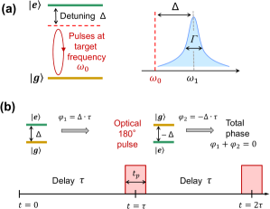
Figure 1: (Color online) (a) Excited state of the two-level system (solid-state emitter) is shifted by random amount $\Delta$ from the desired position $\omega_{0}$, so that the spontaneous emission line (of width $\Gamma$) is centered at $\omega_{1}=\omega_{0}+\Delta$. To shift the line to the target frequency, a sequence of pulses with the carrier frequency $\omega_{0}$ is applied. (b) The optical 180^∘ control pulses are applied periodically, with the interval $\tau$. In the rotating frame, each pulse swaps the ground and the excited state, reversing the detuning $\Delta\to-\Delta$. The total phase accumulated before and after the pulse is nullified, and emission happens as if the detuning was absent, with ZPL centered at $\omega_{0}$.

We model the solid-state emitter as a two-level system, emitting photons in the course of spontaneous transition from the excited state $|e\rangle$ (where the emitter initially is), located at the energy $\hbar\omega_{1}$ above the ground state $|g\rangle$ (below we set $\hbar=1$), see Fig. 1(a). The optical control pulses, each of very short duration $t_{p}$, are applied at the carrier frequency $\omega_{0}$, so it is convenient to work in the rotating-wave approximation (RWA), using the basis rotating with the frequency $\omega_{0}$. The system’s Hamiltonian then has the form

$$H=H_{c}(t)+\frac{\Delta}{2}\sigma_{z}-i\sum_{k=0}^{L-1}g_{k}\left(a^{\dagger}_{k}\sigma^{-}-a_{k}\sigma^{+}\right)+\sum_{k=0}^{L-1}\omega_{k}a^{\dagger}_{k}a_{k},$$ (1)

where $\Delta=\omega_{1}-\omega_{0}$ is the detuning of the ZPL from the target frequency, caused by the random fluctuation in the local strain or charge environment; this detuning is static on the spontaneous emission timescale. The operators $\sigma_{z}=|e\rangle\langle e|-|g\rangle\langle g|$, $\sigma^{+}=|e\rangle\langle g|$, and $\sigma^{-}=(\sigma^{+})^{\dagger}$ describe the emitter, $a_{k}$ is the annihilation operator of the $k$-th photon mode ($L$ modes in total), $g_{k}$ is its coupling strength, and $\omega_{k}$ is its detuning from $\omega_{0}$. The Hamiltonian $H_{c}(t)$, describing the control pulses, can be taken as $H_{c}(t)=(\Omega/2)[\sigma^{+}+\sigma^{-}]$ during the pulses and zero otherwise; for ideal (instantaneous, 180^∘) pulses $\Omega=\pi/t_{p}$ and $t_{p}\to 0$ (experimentally, the optical Rabi frequency $\Omega$ should be large in comparison with the typical $\Delta$). During the pulses, under strong driving $\Omega\ll\Gamma$, the incoherent scattering is dominant Milonni . By including the RWA directly in the Hamiltonian, we assume that $\omega_{1}$ is appropriately renormalized AckerhaltEberly ; RF_KimbleMandel77 , and the non-Markovian effects Milonni ; MarkovApprox_WodEberl in the electromagnetic bath can be neglected.

Our approach is based on a qualitative argument that the frequency of the emitted light is determined by the average rate of phase accumulation AckerhaltEberly ; RF_KimbleMandel77 ; OptPulsesKhitrin between the states $|e\rangle$ and $|g\rangle$ over the time of spontaneous emission $t_{0}$. This is due to the fact that on the timescales short in comparison with the time $t_{0}$ the emitter and the emitted radiation constitute a single coherently evolving quantum system, and the properties of the emitted photon are determined by the whole history of what happened to the emitter during the spontaneous emission time, not only by its instant condition. In our case, by applying the optical control pulses, the average (over the timescale $t_{0}$) rate of the phase accumulation is modified, because each pulse changes $\sigma_{z}$ to $-\sigma_{z}$, so the detuning term $(\Delta/2)\sigma_{z}$ changes its sign, see Fig. 1. If several pulses are applied within the time $t_{0}=1/\Gamma$ then the average detuning is nullified, and the appropriately averaged accumulated phase corresponds to the emission frequency $\omega_{0}$. Below, we assume a simple periodic pulse pattern with the inter-pulse delay $\tau$, as shown in Fig 1(c).

There is a similarity between our approach and the dynamical decoupling (DD) method, which has been used to decouple various quantum systems from their environment DD1 ; DD2 ; DD3 ; DD4 . However, in contrast with the standard optical pulse DD Kurizki ; Walther , the control pulses here do not attempt to cancel the coupling of the qubit to the electromagnetic bath; this would require extremely short Walther inter-pulse delay $\tau\lesssim\omega_{0}^{-1}$ and would suppress emission altogether. Instead, we use the pulses to cancel the detuning, and in this way redirect emission from some electromagnetic modes to others. It may also be possible to achieve the same effect with the continuous control of the emitter, in analogy to the continuous-wave decoupling cwd1 ; cwd2 ; cwd3 ; cwd4 , and consider the sequences with other pulse timings SupMat : this could provide novel ways of modifying the properties of the emitted photons, and constitute an interesting topic for future research.

We characterize the emission spectrum via the number of photons of a given frequency $\omega$: $N_{\omega}(t)=\sum^{\prime}_{k}\langle a_{k}^{\dagger}(t)a_{k}(t)\rangle$, where summation is over the modes with $\omega_{k}=\omega$; note explicit dependence on time $t$. Within RWA description, the relevant frequencies are confined to the vicinity of $\omega_{0}$, so that $\omega_{k}\in[-D,D]$ where $D\ll\omega_{0,1}$ but much larger than all other frequency scales of the problem. Within this region the coupling parameters for all modes are practically constant, $g_{k}=g$ for all $k=0,\dots,L-1$, and the photon density of states $\rho_{\omega}$ is also constant. Thus we choose $\omega_{k}=-D+k\epsilon$, with $\epsilon=2D/(L-1)$; with this choice $\rho_{\omega}=1/\epsilon$. In reality $L\to\infty$, which implies the scaling $g\propto L^{-1/2}$ and $\epsilon\propto L^{-1}$. We also assume fixed polarization of the emitted photons FuEtal ; PfaffHanson . Without control pulses, the solution is the standard Lorentzian emission line RF_Heitler ; AckerhaltEberly centered at $\Delta$ with the width at half maximum $\Gamma=2\pi g^{2}\rho_{\omega}$. Everywhere below we normalize energy and time by $\Gamma$ and $t_{0}=\Gamma^{-1}$, respectively, setting $\Gamma=2$.

We consider the problem using both analytical and numerical approaches in parallel. For analytical treatment we employ the standard approach based on the weak coupling/Markov approximation, used for studying spontaneous decay and resonant fluorescence AckerhaltEberly ; RF_KimbleMandel77 ; RF_Heitler ; MarkovApprox_WodEberl . We use the toggling Heisenberg representation: between the pulses the operators $\sigma_{z}(t)$, $\sigma^{\pm}(t)$, and $a_{k}(t)$ evolve according to standard Heisenberg representation, while the control pulses change the emitter operators $\sigma^{\pm}\to\sigma^{\mp}$, $\sigma^{z}\to-\sigma^{z}$. The corresponding equations of motion for the time-dependent operators after the $n$-th pulse are

$$\dot{a}_{k} = -i\omega_{k}a_{k}+g_{k}\left(\xi_{1}\sigma^{-}+\xi_{2}\sigma^{\dagger}\right)$$ (2)

$$\dot{\sigma}^{-} = -i(-1)^{n}\Delta\sigma^{-}+\sum_{k}g_{k}\xi_{1}a_{k}\sigma_{z}-\sum_{k}g_{k}\xi_{2}a^{\dagger}_{k}\sigma_{z}$$

$$\dot{\sigma}_{z} = -2\sum_{k}g_{k}\left[\xi_{1}a^{\dagger}_{k}\sigma^{-}-\xi_{2}a^{\dagger}_{k}\sigma^{+}-\xi_{2}a_{k}\sigma^{-}+\xi_{1}a_{k}\sigma^{+}\right],$$

where we introduced the periodic functions $\xi_{1}(t)$ and $\xi_{2}(t)$ of period $2\tau$, such that $\xi_{1}(t)=1$ for $t<\tau$ (before the pulse) and $\xi_{1}(t)=0$ for $\tau<t<2\tau$ (after the pulse), while $\xi_{2}(t)=1-\xi_{1}(t)$. The equations of motion (2) can be integrated iteratively between consecutive pulses using the Markovian approximation AckerhaltEberly ; MarkovApprox_WodEberl , and the answer can be obtained in the limit of the large number of pulses; see Supplemental Material SupMat for details.

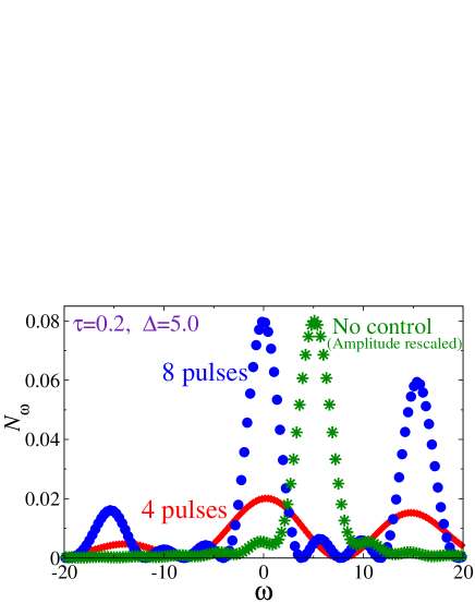
Figure 2: (Color online) Emission profile $N_{\omega}$ in the presence of control pulses, for $\tau=0.2$ and $\Delta=5.0$, after 4 pulses (red diamonds) and 8 pulses (blue circles), as compared with the free spontaneous emission spectrum (green stars). Amplitude of the latter is rescaled for easier comparison with the 8-pulse spectrum.

The analytically calculated fluorescence spectra $N_{\omega}(t)$ are shown in Fig. 2 for $\Delta=5.0$. The free emission (no control pulses) spectrum is compared with the pulse-controlled emission for the inter-pulse delay $\tau=0.2$. The total number of emitted photons increases with the number of pulses, so the amplitude of the no-control spectrum has been rescaled. The spectra agree with our qualitative arguments. The no-control ZPL is centered at $\omega=\Delta$, and only a tiny fraction of emission is present at the target frequency $\omega=0$. In contrast, the control pulses shift the ZPL to the target position. Although additional satellite peaks appear on the sides, about 50% of the spectral weight is successfully moved to $\omega=0$ peak. The emission peaks are wide at $t<t_{0}$, and acquire their natural width $\Gamma$ at longer times.

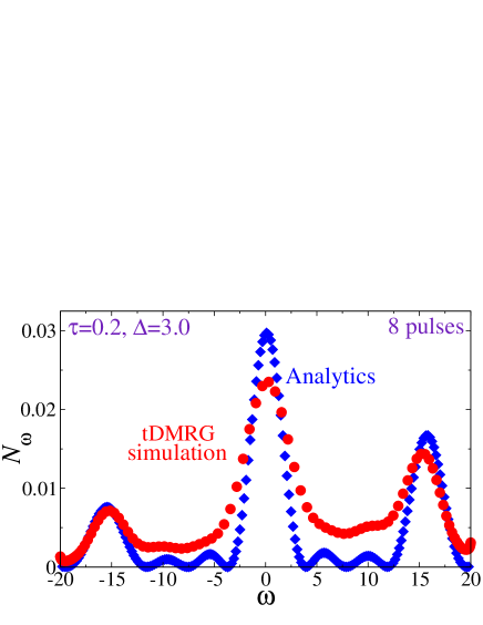
Figure 3: (Color online) Emission profiles $N_{\omega}$ in the presence of control pulses, for $\tau=0.2$ and $\Delta=3.0$, after the 8-th pulse. Blue diamonds represent the analytical results, while the red circles represent the spectrum obtained via time-dependent density matrix renormalization group (tDMRG) simulations. The latter is rescaled by a factor $2/\pi$ in order to take into account different density of the photon modes between the analytical model and the 1-D chain used in tDMRG simulations.

We used numerical simulations to independently check analytical approximation, and to investigate the impact of the pulse imperfections. Each pulse increases the number of total excitations in the system, $n_{ex}=(1+\sigma_{z})/2+\sum_{k}a^{\dagger}_{k}a_{k}$, leading to an exponential increase in the number of relevant states with time. To make the problem tractable, we model the photonic bath in a different way, as a periodic 1-D chain of $L$ harmonic oscillators, with the site 0 coupled to the two-level system (emitter); the corresponding Hamiltonian is

$$H = H_{c}(t)+\frac{\Delta}{2}\sigma_{z}+C\left(\sigma^{+}b_{0}+\sigma^{-}b_{0}^{\dagger}\right)$$ (3)

$$-i(D/2)\sum_{j=0}^{L-1}\left(b_{j}b_{j+1}^{\dagger}-b_{j}^{\dagger}b_{j+1}\right)$$

where $b_{j}^{\dagger}$ and $b_{j}$ are the creation and annihilation operators for a boson at site $j$, respectively. Using Fourier transform of the bosonic operators, it is easy to see that this Hamiltonian is equivalent to Eq. 1, provided that $g_{k}=g=C/\sqrt{L}$ and $\omega_{k}=D\sin{2\pi k/L}$. The latter dispersion relation ensures that the density of states in the vicinity of the emission line (near $\omega_{k}=0$) is also constant, $\rho_{\omega}=[\pi D/L]^{-1}$ (note the double degeneracy of each $\omega_{k}$), and the value of $g$ is adjusted to ensure $\Gamma=2$. The increased density of states at the edges (near $\omega_{k}=\pm D$) is irrelevant because $N_{\omega}(t)$ is small there. Using this model for the photonic bath, the problem can be efficiently solved for large values of $L$ and long times (large number of control pulses), using the time-dependent density matrix renormalization group (tDMRG) method tDMRG using symmetries to reduce the entanglements introduced by the periodic boundary conditions tDMRG2 .

The two methods, analytics vs. tDMRG, are compared in Fig. 3. Good agreement between the two approaches is clearly seen, taking into account the different photon dispersion laws and couplings $g$, the used analytical approximations (weak coupling, large number of pulses), and despite the fact that the parameters ($L=201$, $D=20$, $\rho_{\omega}\approx 3.2$) are far from the ideal quasi-continuous broad spectrum of the photons with $L\gg 1$, $D\gg 1$, and $\rho_{\omega}\gg 1$. In order to account for different spectral density of the photon modes ($\rho_{\omega}=L/(2D)$ for analytics and $\rho_{\omega}=L/(\pi D)$ for tDMRG), the tDMRG simulation results for $N_{\omega}$ are multiplied by a factor $2/\pi$.

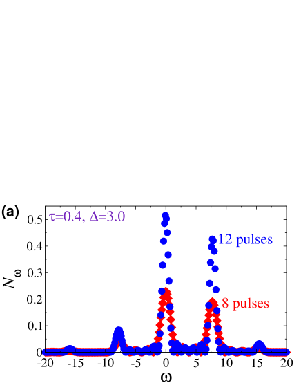
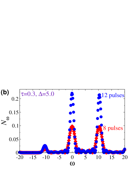
Figure 4: (Color online) Emission profiles $N_{\omega}$ after 8 pulses (red diamonds) and 12 pulses (blue circles). (a) $\tau=0.4$ and $\Delta=3.0$, The satellite peaks at $\omega=\pm\pi/\tau$ and $\pm 2\pi/\tau$ are clearly seen. (b) $\tau=0.4$ and $\Delta=5.0$. Both graphs show that the protocol works for large delays $\tau>1/\Delta$, delivering about 50% of emission to the target frequency.

Dependence of the controlled emission profile on $\Delta$ and $\tau$ is shown in Fig. 4. As expected, the central peak at $\omega=0$ is flanked with the satellite peaks at $\omega=\pm\pi/\tau,\pm 3\pi/\tau,\dots$, since each pulse produces a 180^∘ phase rotation. While the emission into these satellites is unwanted, a large fraction of the spectral power is still retained in the central peak. It is important that our protocol does not require very short inter-pulse delays $\tau$, and works even when $\tau>\Delta^{-1}$, so that even large detunings can be eliminated with moderately spaced pulses. The overall structure of the emission profile remains unchanged even at larger $\tau$. Only, the spectral weight of the central peak decreases for $\tau>2\Delta^{-1}$, while the satellite peak with the frequency closest to $\Delta$ grows SupMat .

Finally, we tested robustness of the approach with respect to two most typical experimental non-idealities, the incomplete rotation during the optical control pulses, and the finite width of the control pulses. We find that a moderate 5^∘ error in the rotation angle does not affect efficiency of the control. In the same way, pulses as wide as $t_{p}=0.05$ (which is 1/4 of the inter-pulse distance $\tau$) remain as efficient as ideal pulses. The corresponding spectra are given in the Supplemental Material. Thus, the requirement of sufficiently large optical Rabi driving, $\Delta\ll\Omega=\pi/t_{p}$, which is needed to ensure that the rotation is close to 180^∘, would not be difficult to satisfy.

By suppressing the spectral diffusion, our protocol improves indistinguishability of the emitted photons. We analyzed the coincidence count rate for the two-photon interference experiments, and the results show significant improvement: informally speaking, about half of the photons become indistinguishable when the pulse control is applied to the emitter; the detailed calculations are presented in the Supplemental Material.

As a specific example, let us consider a nitrogen-vacancy (NV) center in diamond, which has several ZPL separated by 3–5 GHz, corresponding to different excited orbital levels FuEtal ; NVzpls ; NVzpls2 ; RogersNJP ; PfaffHanson . At low temperatures FuEtal ; ZPL_LowT the ZPL has the natural width $\Gamma=2\pi\cdot 16$ MHz, corresponding to the spontaneous decay time $t_{0}=10$ ns. The typical range of the detuning fluctuations $\Delta\sim 5\Gamma=2\pi\cdot 100$ MHz, so that only a small portion of emission occurs at the target frequency $\omega=0$. However, if the control pulses of duration $t_{p}=0.05$ are applied, separated by $\tau=0.3$, then about 50% of the emission goes into the central line at $\omega=0$. For NV centers, this corresponds to the inter-pulse delay $\tau=6$ ns and the pulse width $t_{p}=1$ ns, i.e. optical Rabi driving $\Omega=\pi/t_{p}=2\pi\cdot 0.5$ GHz. These parameters are easily achievable in comparison with the typically used optical Rabi driving of few GHz and sub-ns timing. The modest Rabi driving also limits ionization of NV center, and ensures that other ZPLs, located several GHz away, are not affected.

Concluding, we suggested and analyzed a pulse protocol for suppression of spectral diffusion of the zero-phonon line of a solid-state emitter, which is one of the central problems on the way to implementing the long-range quantum networks with solid-state nodes. We demonstrated feasibility and robustness of the protocol. This approach is simple, does not involve additional levels, and avoids long delays associated with feedback methods (but can also be used along with the latter for fine tuning of the ZPL). More generally, our results show that the pulse control can be efficiently used to manipulate even fast (Markovian) environments, where the typical intra-bath evolution times are far shorter than the inter-pulse delays and pulse durations. Exploring this venue of quantum control can develop solutions for a wide class of problems concerning bosonic and fermionic environments.

We thank L. C. Bassett, R. Hanson, and T. H. Taminiau for inspiring discussions. This work was partially supported by AFOSR MURI program and NSF. The work at Ames Laboratory (design and analysis of the protocol) was supported by the Department of Energy — Basic Energy Sciences under Contract No. DE-AC02-07CH11358. A.E.F. acknowledges NSF support through grant DMR-1339564.

References

- (1) H. J. Kimble, Nature 453, 1023 (2008).
- (2) L.-M. Duan, M. D. Lukin, J. I. Cirac, and P. Zoller, Nature 414, 413 (2001).
- (3) L. Childress, J. M. Taylor, A. S. Sørensen, and M. D. Lukin, Phys. Rev. Lett. 96, 070504 (2006)
- (4) W. Pfaff, B. J. Hensen, H. Bernien, S. B. van Dam, M. S. Blok, T. H. Taminiau, M. J. Tiggelman, R. N. Schouten, M. Markham, D. J. Twitchen, R. Hanson, Science 345, 532 (2014).
- (5) H. Bernien, B. Hensen, W. Pfaff, G. Koolstra, M. S. Blok, L. Robledo, T. H. Taminiau, M. Markham, D. J. Twitchen, L. Childress and R. Hanson, Nature 497, 86 (2013).
- (6) W. B. Gao, P. Fallahi, E. Togan, A. Delteil, Y. S. Chin, J. Miguel-Sanchez, and A. Imamoğlu, Nature Comm. 4, 2744 (2013).
- (7) S. D. Barrett and P. Kok, Phys. Rev. A 71, 060310(R), (2005).
- (8) E. Togan, Y. Chu, A. S. Trifonov, L. Jiang, J. Maze, L. Childress, M. V. G. Dutt, A. S. Sørensen, P. R. Hemmer, A. S. Zibrov, and M. D. Lukin, Nature 466, 730 (2010).
- (9) B. B. Buckley, G. D. Fuchs, L. C. Bassett, and D. D. Awschalom, Science 330, 1212 (2010).
- (10) A. Batalov, V. Jacques, F. Kaiser, P. Siyushev, P. Neumann, L. J. Rogers, R. L. McMurtrie, N. B. Manson, F. Jelezko, and J. Wrachtrup, Phys. Rev. Lett. 102, 195506 (2009).
- (11) C. Santori, D. Fattal, J. Vučković, G. S. Solomon, and Y. Yamamoto, Nature 419, 594 (2002).
- (12) J. R. Schaibley, A. P. Burgers, G. A. McCracken, L.-M. Duan, P. R. Berman, D. G. Steel, A. S. Bracker, D. Gammon, and L. J. Sham, Phys. Rev. Lett. 110, 167401 (2013)
- (13) S. G. Carter, T. M. Sweeney, M. Kim, C. S. Kim, D. Solenov, S. E. Economou, T. L. Reinecke, L. Yang, A. S. Bracker, and D. Gammon, Nature Photonics 7, 329 (2013).
- (14) J. C. Lee, I. Aharonovich, A. P. Magyar, F. Rol, and E. L. Hu, Opt. Express 20, 8892 (2012).
- (15) A. Faraon, P. E. Barclay, C. Santori, K.-M. C. Fu, and R. G. Beausoleil, Nature Photonics 5, 301 (2011)
- (16) K.-M. C. Fu, C. Santori, P. E. Barclay, L. J. Rogers, N. B. Manson, and R. G. Beausoleil, Phys. Rev. Lett. 103, 256404 (2009).
- (17) L. C. Bassett, F. J. Heremans, C. G. Yale, B. B. Buckley, and D. D. Awschalom, Phys. Rev. Lett. 107, 266403 (2011).
- (18) J. Hansom, C. H. H. Schulte, C. Matthiesen, M. J. Stanley, and M. Atatüre, Appl. Phys. Let. 105, 172107 (2014)
- (19) V. M. Acosta, C. Santori, A. Faraon, Z. Huang, K.-M. C. Fu, A. Stacey, D. A. Simpson, K. Ganesan, S. Tomljenovic-Hanic, A. D. Greentree, S. Prawer, and R. G. Beausoleil, Phys. Rev. Lett. 108, 206401 (2012).
- (20) J. H. Prechtel, A. V. Kuhlmann, J. Houel, L. Greuter, A. Ludwig, D. Reuter, A. D. Wieck, and R. J. Warburton, Phys. Rev. X 3, 041006 (2013).
- (21) A. V. Kuhlmann, J. Houel, A. Ludwig, L. Greuter, D. Reuter, A. D. Wieck, M. Poggio, and R. J. Warburton, Nature Physics 9, 570 (2013)
- (22) S. A. Crooker, J. Brandt, C. Sandfort, A. Greilich, D. R. Yakovlev, D. Reuter, A. D. Wieck, and M. Bayer, Phys. Rev. Lett. 104, 036601 (2010).
- (23) C. Matthiesen, M. J. Stanley, M. Hugues, E. Clarke, and M. Atatüre, Sci. Reports 4, 4911 (2014)
- (24) C. Santori, D. Fattal, K.-M. Fu, P. E. Barclay, and R. G. Beausoleil, New J. Phys. 11 123009 (2009).
- (25) Y. He, Y.-M. He, Y.-J. Wei, X. Jiang, M.-C. Chen, F.-L. Xiong, Y. Zhao, C. Schneider, M. Kamp, S. Höfling, C.-Y. Lu, and J.-W. Pan, Phys. Rev. Lett. 111, 237403 (2013).
- (26) C. Matthiesen, M. Geller, C. H. H. Schulte, C. Le Gall, J. Hansom, Z. Li, M. Hugues, E. Clarke, and M. Atatüre, Nature Comm. 4, 1600 (2013).
- (27) C. Matthiesen, A. N. Vamivakas, and M. Atatüre, Phys. Rev. Lett. 108, 093602 (2012).
- (28) P. L. Knight and P. W. Milonni, Phys. Reports 66, 21 (1980).
- (29) J. R. Ackerhalt and J. H. Eberly, Phys. Rev. D 10, 3350 (1974).
- (30) H. J. Kimble and L. Mandel, Phys. Rev. A 15, 689 (1977).
- (31) K. Wódkiewicz and J. H. Eberly, Ann. Phys. 101, 574 (1976).
- (32) J.-S. Lee, M. A. Rohrdanz, and A. K. Khitrin, J. Phys. B 41 045504 (2008).
- (33) L. Viola, E. Knill, and S. Lloyd, Phys. Rev. Lett. 82, 2417 (1999).
- (34) M. J. Biercuk, H. Uys, A. P. Vandevender, N. Shiga, W. M. Itano, and J. J. Bollinger, Nature 458, 996 (2009).
- (35) V. V. Dobrovitski, G. D. Fuchs, A. L. Falk, C. Santori, and D. D. Awschalom, Ann. Rev. Cond. Matter Physics 4, 23 (2013).
- (36) H. Bluhm, S. Foletti, I. Neder, M. Rudner, D. Mahalu, V. Umansky, and A. Yacoby, Nat. Phys. 7, 109 (2011).
- (37) A. G. Kofman and G. Kurizki, Nature 405, 546 (2000).
- (38) G. S. Agarwal, M. O. Scully, and H. Walther, Phys. Rev. Lett. 86, 4271 (2001).
- (39) P. Facchi, D. A. Lidar, and S. Pascazio, Phys. Rev. A 69, 032314 (2004).
- (40) J.-M. Cai, B. Naydenov, R. Pfeiffer, L. P. McGuinness, K. D. Jahnke, F. Jelezko, M. B. Plenio, and A. Retzker, New J. Phys. 14, 113023 (2012).
- (41) X. Xu, Z. Wang, C. Duan, P. Huang, P. Wang, Y. Wang, N. Xu, X. Kong, F. Shi, X. Rong, and J. Du, Phys. Rev. Lett. 109, 070502 (2012)
- (42) D. A. Golter, T. K. Baldwin, and H. Wang, Phys. Rev. Lett. 113, 237601 (2014)
- (43) W. Heitler, The Quantum Theory of Radiation (Oxford University Press, London, 1960).
- (44) See Supplemental Material [url], which includes Refs. CohenTann –LZK .
- (45) C. Cohen-Tannoudji, J. Dupont-Roc, and G. Grynberg, Atom-Photon Interactions. Basic Processes and Applications (John Wiley & Sons, Inc., New York, 1992).
- (46) M. O. Scully and M. S. Zubairy, Quantum Optics (Cambridge University Press, New York, 1997).
- (47) B. R. Mollow, Phys. Rev. 188, 1969 (1969).
- (48) A. Kiraz, M. Atatüre, and A. Imamoğlu, Phys. Rev. A 69, 032305 (2004).
- (49) R. Loudon, The Quantum Theory of Light (Clarendon Press, Oxford, 1983).
- (50) D. A. Lidar, P. Zanardi, K. Khodjasteh, Phys. Rev. A 78, 012308 (2008).
- (51) S.R. White and A.E. Feiguin, Phys. Rev. Lett. 93, 076401 (2004).
- (52) A. E. Feiguin and C. A. Büsser, Phys. Rev. B 84, 115403 (2011).
- (53) N. B. Manson, J. P. Harrison, and M. J. Sellars, Phys. Rev. B 74, 104303 (2006).
- (54) L. J. Rogers, R. L. McMurtrie, M. J. Sellars, and N. B. Manson, New J. Phys. 11, 063007 (2009).
- (55) Y. Shen, T. M. Sweeney, and H. Wang, Phys. Rev. B 77, 033201 (2008).