An interplay of migratory and division forces as a generic mechanism for stem cell patterns

Résumé

In many adult tissues, stem cells and differentiated cells are not homogeneously distributed: stem cells are arranged in periodic "niches", and differentiated cells are constantly produced and migrate out of these niches. In this article, we provide a general theoretical framework to study mixtures of dividing and actively migrating particles, which we apply to biological tissues. We show in particular that the interplay between the stresses arising from active cell migration and stem cell division give rise to robust stem cell patterns. The instability of the tissue leads to spatial patterns which are either steady or oscillating in time. The wavelength of the instability has an order of magnitude consistent with the biological observations. We also discuss the implications of these results for future in vitro and in vivo experiments.

A fascinating property of developing biological tissues is the ability of initially identical cells to differentiate and form robust macroscopic patterns. This raises the important question of the transmission of biological information on scales much larger than the cell size, and of the origin of the positional information. The pioneering work of Turing 1 has shown that diffusion-reaction mechanisms are a generic way of to create self-organized patterns 2 ; 2b ; 5 ; 5b ; 7c , and the discovery of morphogens has stimulated a renewed interest for these ideas 7d . Nevertheless, their applicability in biology remains limited, and most of the patterns that have been studied have been shown to result rather from short range cellular inhibition than from a long-range diffusion gradient 3 .

On the other hand, mechanical stress is increasingly being recognized as an important regulator of tissue homeostasis and of many cellular events such as cell division, differentiation and death 8 ; 9 ; 10 ; 11 ; 12 ; 12a . It is therefore of major importance to understand the coupling between the mechanical state of a tissue and the regulation and patterning of stem cells. Although long-ranged morphogens gradients play a crucial role in differentiation 7d , mechanical signaling is long-range and propagates fast, which makes it a robust candidate for patterning as well. On the other hand, collective cell migration in cultured cells creates large stresses, which propagate on macroscopic scales 13 , in a similar manner to the flocking studied by Toner and Tu 13aa . Nevertheless, the contribution of active cell migration to the homeostasis and patterning of stem cells in tissues has not, to the best of our knowledge, been investigated in the past. In many instances such as in the skin and intestinal epithelia, stem cells are not homogeneously distributed, but are rather located in periodically spaced niches, where they divide and give rise to differentiated cells. Here, we build up a theoretical framework to investigate simultaneously cell division, differentiation and active migration in a tissue. We show that the interplay between the stresses generated by division and migration is a generic route toward tissue patterning. Indeed, as the differentiated cells actively migrate out of the niches, they create stress gradients that maintain the niche under tension, a mechanical feedback that has been shown to enhance cell division and influence stem cell fate. This creates a self-reinforcing loop, where stem cells produce differentiated cells, which migrate away, enabling yet more stem cell divisions.

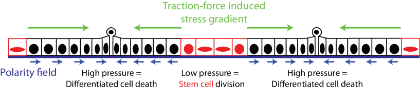
Figure 1: Sketch of our model. Differentiate cells actively migrate out of the stem cell compartment, putting it under tension. Stem cell give rise to differentiate cells which actively migrate out of the stem cell compartment. By doing so, they put under tension the stem cell compartment, enabling more stem cell division, and actively maintaining the phase separation.

We consider only two cell types: stem cells divide and differentiate, but cannot actively migrate, whereas differentiated cells actively migrate but cannot divide 15 . Cells actively migrate by exerting lamellipodial forces on the substrate in a polarized manner. We model this migratory polarization by a vector $\bf{p}$, pointing towards the front of the cell (i.e. from the center of mass of the cell towards the lamellipodia). There are therefore four hydrodynamic variables: the densities of stem and differentiated cells $\rho_{s}$ and $\rho_{d}$, the hydrodynamic velocity of the mixture $\bf{v}$ and the polarization field $\bf{p}$. The conservation equations for cell densities read:

$$\partial_{t}\rho_{s}+\nabla(\rho_{s}{\bf v_{s}}) = k(\rho_{s},\rho_{d})\rho_{s}-k_{d}\rho_{s}$$

$$\partial_{t}\rho_{d}+\nabla(\rho_{d}{\bf v_{d}}) = k_{d}\rho_{s}-k_{a}\rho_{d}$$ (1)

where $k$, $k_{d}$ are respectively the division and differentiation rate of stem cells and $k_{a}$ the loss rate of differentiated cells. At homeostasis, in the absence of cell flow ($v=0$), the cell densities $\rho_{s}^{h}$ and $\rho_{d}^{h}$ are uniform. However, Eqns. 1 are unstable if there is no negative feedback preventing infinite growth of tissues as soon as $k>k_{d}$. Following previous works, we assume that cell division is regulated by the total cell density and expand the division rate at linear order around the homeostatic state:

$$k-k_{d}=-\frac{1}{\tau_{s}}(\rho_{s}+\rho_{d}-1)$$

setting $\rho_{s}^{h}+\rho_{d}^{h}=1$ without loss of generality. Finally, one needs to specify a constitutive equation for the relative flux $J$. We assume it is a diffusive current caused by gradients in the fraction of stem cells: $J=D\nabla\frac{\rho_{s}}{\rho_{s}+\rho_{d}}$, $D$ being a diffusion constant. In the following, we assume $D=0$ for the sake of simplicity, although a finite value of D simply shifts the instability threshold without changing the physics of the instability.

We use the theoretical framework of Ref.16 for the dynamics of two cell populations of respective densities and local velocities $\rho_{\alpha}$ and $v_{\alpha}$ ($\alpha=s,d$). The barycentric velocity ${\bf v}$ and the relative flux ${\bf J}$ are defined by ${\bf v_{s}}={\bf v}+{\bf J}/\rho_{s}$ and ${\bf v_{d}}={\bf v}-{\bf J}/\rho_{d}$. The barycentric velocity is then determined from force balance:

$$\partial_{i}\sigma_{ij}=\xi(\rho_{s},\rho_{d})(v_{j}-V(\rho_{s},\rho_{d})p_{j})$$ (2)

where $\sigma_{ij}$ is the stress tensor, $\xi$ is the friction coefficient of the cell mixture on the solid substrate. The active migration speed $V$ is written as $V=V_{0}\phi$, to first order, with $V_{0}$ and $\phi=\frac{\rho_{d}}{\rho_{s}+\rho_{d}}$ respectively the migration speed and fraction of differentiated cells. This frictional force assumes that the cells are resting on a solid substrate, which is the case for most epithelial cells resting on a stroma, and that only differentiated cells can actively migrate, a hypothesis which has biological grounds, as discussed in Ref. 15

On timescales larger than the cell turnover time, tissues have been shown to behave as viscous fluids 18 , yielding a constitutive equation for the stress: $\sigma_{ij}=-\Pi\delta_{ij}+2\eta_{1}v_{ij}+\eta_{2}\partial_{k}v_{k}\delta_{ij}$, where $\eta_{1}$ and $\eta_{2}$ are the shear and bulk viscosities respectively, $v_{ij}=1/2(\partial_{i}v_{j}+\partial_{j}v_{i}-2/3\partial_{k}v_{k}\delta_{ij})$ and $\Pi$ the pressure in the tissue. We redefined $2\eta_{1}+\eta_{2}=\eta$ in the following, which is the only relevant quantity in the one-dimensional case that we study in the main text. In order to calculate the pressure and the polarization fields, we follow Ref.17 and treat the tissue as a quasi-equilibrium mixture close to the homeostatic state. We define the relative dimensionless concentrations $\delta\rho_{\alpha}=\frac{\rho_{\alpha}-\rho_{\alpha}^{h}}{\rho_{\alpha}^{h}}$ and expand the effective energy density, keeping all quadratic terms allowed by symmetry and of first order close to equilibrium. Moreover, we make the crucial assumption that differentiated cells have no spontaneous polarity, and expand the energy around ${\bf p}={\bf 0}$:

$$f=\frac{1}{2\chi_{s}}\delta\rho_{s}^{2}+\frac{1}{2\chi_{d}}\delta\rho_{d}^{2}+\frac{1}{\chi}\delta\rho_{s}\delta\rho_{d}+\frac{\nu}{2}p^{2}\\ +\frac{K}{2}(\partial_{\alpha}p_{\beta})(\partial_{\alpha}p_{\beta})+w(\delta\rho_{s},\delta\rho_{d})\partial_{\alpha}p_{\alpha}$$ (3)

$\chi_{s}$, $\chi_{d}$, $\chi$ are the compressibilities associated with the mixture, $\nu$ is a positive constant, $K$ is the Frank constant of the polarization field (using the standard one-constant approximation) and $w(\delta\rho_{s},\delta\rho_{d})$ can be expanded to first order around the homeostatic state: $w(\delta\rho_{s},\delta\rho_{d})=w_{0}+w_{s}\delta\rho_{s}+w_{d}\delta\rho_{d}$. This last term exists by symmetry for polar nematics and couples the polarity field to the density. $w_{s}$ and $w_{d}$ are coefficients which, because the system is active, can have any signs, and represent the magnitude of the coupling between polarity and the gradients of stem and differentiated cell densities, respectively.

Then the polarization equation reads:

$$\gamma\partial_{t}\textbf{p}=-\frac{\delta F}{\delta\textbf{p}}=-\nu\textbf{p}+K\Delta\textbf{p}+w_{s}\nabla\rho_{s}+w_{d}\nabla\rho_{d}$$ (4)

where $\gamma$ is a rotational viscosity.

We now rewrite the equations for the evolution of the tissue in dimensionless units using $\tau=\gamma/\nu$ as the time unit and $L=(\eta/\xi)^{1/2}$ as the length unit.

$$\partial_{t}\rho_{s}+\nabla(\rho_{s}\textbf{v})=-(\rho_{s}+\rho_{d}-1)\rho_{s}/\tau_{s}\\ \partial_{t}\rho_{d}+\nabla(\rho_{d}\textbf{v})=\epsilon\left(\rho_{s}-\rho_{s}^{h}\rho_{d}\right/\rho_{d}^{h})/\tau_{s}\\ \partial_{t}\textbf{p}=-\textbf{p}+K\Delta\textbf{p}+(w_{d}/\nu)\nabla\rho_{d}+(w_{s}/\nu)\nabla\rho_{s}\\ \textbf{v}-V_{0}\phi\textbf{p}=\Delta\textbf{v}-\nabla\rho_{s}/\chi_{s}-\nabla\rho_{d}/\chi_{d}-W\Delta{\bf p}$$ (5)

where $1/\chi_{\alpha}+1/\chi=1/{\tilde{\chi}}_{\alpha}$, $\epsilon=\tau_{s}k_{d}$, $(K\xi)/(\nu\eta)={\tilde{K}}$, $\tau_{s}/\tau={\tilde{\tau}}_{s}$, $V_{0}\tau/L={\tilde{V}}_{0}$, $\chi_{\alpha}L^{2}\xi/\tau={\tilde{\chi}}_{\alpha}$ and $W=(w_{s}+w_{d})/(L^{2}v_{1}\xi)$ and we have omitted all ${\tilde{\ }}$ symbols.

In the following, we assume for a sake of simplicity that the compressibility of the two cell types are identical, and define $\chi=\chi_{s}=\chi_{d}$. We perform a linear stability analysis of the homeostatic state of Eqns.5, i.e. $v=0,\bf{p}=0$, $\rho_{i}=$ constant, by looking for the evolution of Fourier modes of wave vector $\bf q$. We define a $3$-dimensional vector ${\bf X}(\delta\rho_{s},\delta\rho_{d},{\bf p})$ and denote by ${\tilde{\bf X}}({\bf q})$ its Fourier transform. The linearization of Eqns.5 is written in the form ${\partial_{t}}{\tilde{\bf X}}=M{\tilde{\bf X}}$ with M defined as

$$M=\left({\begin{array}[]{ccc}-(1-\phi)(\frac{1}{\tau_{s}}+\frac{1}{\chi}\frac{q^{2}}{1+q^{2}})&-(1-\phi)(\frac{1}{\tau_{s}}+\frac{1}{\chi}\frac{q^{2}}{1+q^{2}})&-\frac{iq}{1+q^{2}}V_{0}\phi(1-\phi)-\frac{iq^{3}}{1+q^{2}}W\\ \epsilon\frac{1}{\tau_{s}}-\phi\frac{1}{\chi}\frac{q^{2}}{1+q^{2}}&-(\frac{1}{\phi}-1)\epsilon\frac{1}{\tau_{s}}-\phi\frac{1}{\chi}\frac{q^{2}}{1+q^{2}}&-\frac{iq}{1+q^{2}}V_{0}\phi^{2}-\frac{iq^{3}}{1+q^{2}}W\\ iqw_{s}&iqw_{d}&-1-Kq^{2}\end{array}}\right)$$ (6)

The signs of the eigenvalues of the stability matrix $M$ determine the stability of the tissue. If an eigenvalue $s_{i}(i=1,2,3)$ becomes positive above a threshold $V_{c}$ of migratory speed $V_{0}$, a perturbation grows at the most unstable wavevector $q_{c}$.

The solution of this system is rather complicated in the general case, but we deduce below the general behavior from special cases and numerical calculations of the eigenvalues. The coupling between polarization and density drives the instability via two terms : $w_{i}$ promotes an instability at a finite wavelength, and $W$, which is a higher order term, promotes an instability at vanishing wavelength ($q_{c}\to\infty$) above a threshold $W_{c}$. This instability is unphysical, and higher order terms that would stabilize the tissue must be included if $W>W_{c}$. In the following, we study only the limit $W=0$. The results would be qualitatively similar for any $W<W_{c}$ since, far from the threshold, the wavelength of the instability is insensitive to the value of $W$.

Moreover, the eigenvalue associated with the polarization is always negative. Therefore, we can assume without qualitatively modifying the results, that the polarization equation relaxes instantly, and reduce $M$ to a $(2\times 2)$ matrix (see SI Text for details). Our analysis shows that either one or two eigenvalues of the stability matrix can be positive and therefore the bifurcation is of co-dimension 2. We distinguish three types of instabilities: the homogeneous phase is unstable if either only one eigenvalue is real positive, two complex conjugate eigenvalues have a positive real part or two eigenvalues are real positive. We plot an illustrative example of the evolution of the eigenvalues in the Supplementary Text.

Interestingly nevertheless, the wavelength of the stationary spatial instability depends only on the parameters $K$, $\chi$ and $\tau_{s}$:

$$\lambda_{c}=2\pi\left(K(\tau_{s}+\chi)/\chi\right)^{1/4}$$ (7)

In the following, we choose for simplicity the example were $\chi=1$, $K=1$ and $\phi=0.5$. One can give exact expressions for the instability threshold. In order to simplify the analysis, we define $A=\frac{1}{\chi}\frac{q^{2}}{1+q^{2}}$ and $B=\frac{V_{0}\phi q^{2}}{(1+Kq^{2})(1+q^{2})}$.

A first transition occurs when only one eigenvalue becomes real positive if the active speed exceeds a critical value $V_{c}^{1}$, such as $B$ is:

$$V_{c}^{1}\propto B=\frac{1}{w_{d}(1+\epsilon)-w_{s}(1-\frac{1-\phi}{\phi}\epsilon)}\left(A+\frac{1}{\tau_{s}}\right)\frac{\epsilon}{\phi}$$ (8)

As expected, the instability threshold increases monotonously with the turnover rates $\tau_{s}$. Increasing the coupling $w_{d}$ decreases the threshold. This criterion also indicates that the value $\epsilon_{c}=\frac{\phi}{1-\phi}$ plays a special role. For $\epsilon<\epsilon_{c}$, increasing $|w_{s}|$ (if $w_{s}<0$, i.e. towards more negative values) decreases the threshold of the instability. As we expect the turnover of differentiated cells to be much faster than the turnover of stem cells ($\epsilon\ll 1$), this is likely the more realistic limit. In the following, we concentrate on this limit $\epsilon<\epsilon_{c}$. At this transition, the positive eigenvalue is real and has no imaginary part, so that we expect formation of steady patterns. In the Supplementary Text, we examine the case $\epsilon>\epsilon_{c}$, which yields to a global phase separation with regions rich in both stem and differentiated cells, and regions poor in both.

A second transition occurs when the two eigenvalues are complex conjugate and their reals parts become positive simultaneously. This occurs only above a critical value of the speed $V^{2}_{c}$. At this transition, the presence of two complex conjugate eigenvalues suggest the appearance of spatial patterns oscillating in time, with a frequency given by the imaginary part of the eigenvalue. For this second, non-stationary bifurcation, the most unstable wavelength $q_{2}$ is defined by $q_{2}^{4}=\frac{\chi}{K}\frac{1}{\chi+\bar{\tau_{s}}}$ where $\bar{\tau_{s}}=\frac{\tau_{s}}{1-\phi}\frac{\phi}{\phi+\epsilon}$. One should note the resulting wavelength can become very different from the one of the first transition, in particular if one cell type is in large excess compared to the other ($\phi\to 1$ or $\phi\to 0$).

The critical velocity speed at the threshold $V_{c}^{2}$ is such that for $q=q_{2}$:

$$V_{c}^{2}\propto B=\frac{1}{w_{s}\phi+(1-\phi)w_{d}}\left(A+\frac{1-\phi}{\tau_{s}}(\frac{\epsilon}{\phi}+1)\right)$$

which is always a decreasing function of both couplings $w_{s}$ and $w_{d}$.

Importantly, there is always an intersection point between the two transition curves. Indeed, the equation $V^{1}_{c}=V^{2}_{c}$ always has a solution, which defines a critical point $w_{sc}$ in the $(w_{s},V_{0})$ space for any value of $w_{d}$. One can usefully define $\Delta=w_{s}-w_{d}$ as the difference of the two couplings, and see that the transition occurs for $\Delta w=0$ (see SI Text). At this critical point, both eigenvalues have vanishing real and imaginary parts at the same time, characteristic of a Bogdanov-Takens bifurcation.

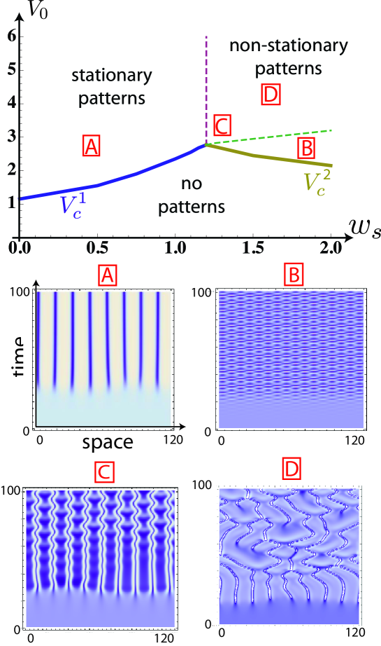
Figure 2: Phase diagram of the patterning instability in 1 dimension. Stationary patterns arises above a critical value of the active migration speed $V_{0}$, but also non-stationary patterns above a critical value of the coupling $w_{s}$. We display representative examples of the four phases of the diagram (bellow), showing kymographs of the evolution of the stem cell concentration.

Moreover, for $\epsilon<\epsilon_{c}$, $V^{1}_{c}$ is an increasing function of $w_{s}$ whereas $V^{2}_{c}$ is a decreasing function of $w_{s}$. Therefore, we expect a reentry phenomena due to this non-monotonous threshold for the instability: the homogeneous system is stable for intermediate values of $w_{s}$, and unstable both for small (steady patterns) and large (unsteady patterns) values of $w_{s}$, as can be seen by following a horizontal line in the phase diagram Fig. 2.

We now concentrate on the orders of magnitude of the various parameters. In various epithelial tissues 12 ; 13 , the typical migration speed is $V_{0}=10\mu m/h$, the typical density is $\rho_{0}=0.01$ cell$/\mu m^{2}$, the typical division time of stem cells is $\tau_{s}=24h$ and the typical fraction of differentiated cell is $\phi\approx 0.9$. Moreover, measurements suggest $\eta_{3D}\approx 10^{5}Pa.s$ 18 and $\zeta=10^{10}Pa.m^{-1}$ 18a . If $h=10\mu m$ is the characteristic height of a cell, then $L=(\eta_{3D}h/\zeta)^{1/2}=10\mu m$, agreeing with measurements 19 in the Drosophila scutellum. Finally, observations on actin dynamics in epithelial sheets and experiments on cells under tension 16a suggest a characteristic protrusion time $\tau=1-2min$. The typical compressibility is the inverse of the typical pressure exerted by tissues: $\chi\approx 10^{-3}Pa^{-1}$ 20 .

We can then evaluate several of the rescaled quantities: $\frac{1}{\chi}\approx 10$, $\tau_{s}\approx 10^{3}$, $V_{0}\approx 1$. Based on available evidence, we suppose that the interaction between two polarization vectors is only effective a few cell distances, leading to $K\approx 1$. This predicts a critical wavelength of the pattern: $\lambda_{c}\approx 600\text{ }\mu m$, close to the values observed both in the intestinal and skin epithelia 15 ; 2 . By construction, we have the polarity field $\textbf{p}\sim 1$, and since $\textbf{p}\propto w_{s,d}\textbf{q}$, it imposes $w_{s,d}\approx 10$. Furthermore, imposing a turnover rate $\epsilon\approx 0.1-1$, we can calculate numerically the typical value of the critical migration speed, $V_{c}\approx 0.1-1$, close to the estimated active migration speed: the stress exerted by differentiated cells is large enough to trigger the instability.

In order to go beyond our stability analysis, we performed a full numerical integration of Eq. 5. We show the results in 1 dimension on Fig. 3, as well as in 2 dimensions on Fig. 4. We started with $w_{s}=0$, $w_{d}=1$ and increasing values of the active migration rate $V_{0}$. The result is plotted on Fig. 3 and displays phase separation and formation of steady state stem cell patterns for high values of $V_{0}$. The wavelength calculated from this simulation agrees perfectly with the wavelength deduced from our linear stability analysis. The values that we have used for this simulation are $\chi=1$, $K=1$ and $\phi=1/2$, $\epsilon=0.2$, $\tau=10$, with four values of $V_{0}$ indicated on the figure.

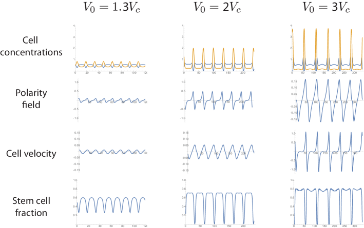
Figure 3: Numerical integration of our equations in 1 dimension, for $\epsilon=0.2$, demonstrating the formation of stem cell pattern for high values of the active migration rate $V_{0}$. We plot the stem/differentiated cell concentration (reps. in orange and blue on the top row) as well as the polarity field $p$, the cell barycentric velocity $v$ and and the stem cell fraction (in blue on the second, third and fourth row respectively).

In two-dimensions, hexagonal patterns are observed for all the values we tested, and we show an example for $V_{0}=1.2V_{c}$. We neglected the bulk viscosity in the simulation, although we verified that including it did not yield qualitatively different results. We give in Fig. 4 the intensity plots for the densities of stem and differentiated cells, as well as the polarity field, which goes from stem cell-rich to stem-cell poor regions.

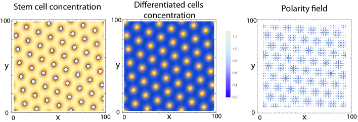
Figure 4: Numerical integration of our equations in 2 dimensions, demonstrating the formation of stem cell pattern for high values of the active migration rate $V_{0}$. We show a density plot of the stem cell and differentiated cell concentration profile (left and center), and the polarity field (right) as a function of the two spatial coordinates. The parameters we use, as in Fig. 3 are $\chi=1$, $K=1$ and $\phi=1/2$, $\epsilon=0.2$, $\tau=10$ and $V_{0}=1.2V_{c}$.

We also explored the phase diagram in the plane ($w_{s}$, $V_{0}$) for a constant value of $w_{d}=1.25$, and drew the numerical transition lines from a homogeneous to a patterned state (see Fig. 2), for many values of $w_{s}$, which agree perfectly with the previous analytical criteria. Patterns can only be seen above a critical value of $V_{0}$, which depends on $w_{s}$. Moreover, below a critical value of the coupling $w_{s}$, only steady spatial patterns are formed (Fig. 2A), whereas above, we observe the appearance of standing waves of finite spatial and temporal frequency (Fig. 2B), as predicted by our bifurcation analysis. The numerical transition lines match quantitatively our analytical prediction for $V_{c}^{1}$ and $V_{c}^{2}$.

As shown in Fig. 2, there is a complex zoology of non-stationary patterns, when the active migration speed is increased further, ranging from caged oscillation of stem cell compartments to chaotic motion. These patterns are not accessible by a linear stability analysis, and a full non-linear treatment would be necessary, but is well beyond the scope of this paper. Physically, this corresponds to the fact that for large positive values of both $w_{s}$ and $w_{d}$, the cell polarity field is oriented by two gradients in opposite directions ($\rho_{s}$ and $\rho_{d}$). Therefore, the cells alternate between the two cues, ans this gives rise to complex spatio-temporal patterns (Fig. 2C-D).

In this article, we have presented a simple analytical model to describe epithelial tissues and stem cell patterns. Our model is nevertheless general for any mixture of particles actively dividing and migration, since we considered all hydrodynamical coupling allowed by symmetry, our only assumption being that there was no spontaneous polarisation in the homogeneous state. The patterns we studied reflect a compromise between stresses exerted by the migration of differentiated cells and the division of stem cells. Above a threshold value for the active migration velocity, a positive feedback loop drives the partial phase separation of the tissue into stem cell-rich and stem cell poor regions, which are either stationary or dynamic in time. This is due to an effective collective migration effect, where migration polarity is coupled to the gradient of cell concentrations in the tissue. Complete phase-separation has been found to be quite general in active self-propelled one-component systems 45 , although here, turnover prevents complete phase separation, yielding robust patterns.

This mechanism is in contrast with previous mechanism of patterning, which rely on diffusion, either of a contractile specie in active fluids 12 or of a morphogen in the classical Turing framework 1 . One advantage of our mechanism is that it does not require a given genetic pathway, but only rather two ingredients that are already known to exist generically in tissues : coupling of neigbouring cells polarity fields, and cell turnover. This could be a source of robustness, in addition to not requiring diffusion of a molecule over long ranges, which might be challenging be achieve in many situations.

In our framework, the pressure in the epithelium would follow the same pattern as the cell concentration. A straightforward extension of our model would therefore be to consider a two dimensional description of the epithelium flows on an arbitrarily curved substrate, and to study the corresponding buckling instability 22b . This is particularly topical given a recent combination of theory and experiment suggesting that stem cell fate was linked to the local curvature of the epithelium and underlying stroma 22c .

Our modelling therefore suggests two future research directions. On the one hand, experiments would be needed to verify our analytical prediction on the influence of active migration velocity on patterning. In vivo, this could be achieved by inhibiting actin cell migration through specific Arp2/3 inhibitors 22a to test whether this disrupts stem cell niches. In vivo, traction force microscopy 13 could be used on cultured reconstituted epidermis, which exhibit stem cell patterns 2 . The measured active migration field could then be correlated in time and space with live-markers for stem cells, in order to test our predictions, as well as measuring the coupling constants $w_{i}$. The existence of oscillating patterns could also be tested in the same system, as well as the dependency of the pattern wavelength on division rate. On the other hand, more theoretical work would be necessary to include in our description various non-linear terms which could prove especially important for patterning.

- (1) Turing, A. M. (1952). Phil. Trans. Royal Soc. B, 237(641), 37-72.
- (2) Klein, A. M. et al (2011). J Royal Soc Inter, rsif20110240.
- (3) Maini, P. K. (2004). Mathematics Today, 40(4), 140-141.
- (4) Cates, M. E., Marenduzzo, D., Pagonabarraga, I., and Tailleur, J. (2010). Proc Nat Acad Sc, 107(26), 11715-11720.
- (5) Sankararaman, S., and Ramaswamy, S. (2009) Phys Rev Lett, 102(11), 118107, 1-118107.
- (6) Bois, J. S., Julicher, F., and Grill, S. W. (2011). Phys Rev Lett, 106(2), 028103.
- (7) Wolpert, L. (1969). J. Theor. Biol., 25(1), 1-47.
- (8) Inaba, M., Yamanaka, H., and Kondo, S. (2012). Science, 335(6069), 677-677.
- (9) Shraiman, B. I. (2005). Proc Nat Acad Sc, 102(9), 3318-3323.
- (10) Montel, F. et al (2011). Phys Rev Lett, 107(18), 188102.
- (11) Streichan, S et al. (2014). Proc Nat Acad Sc, 111(15), 5586-5591.
- (12) Sun, Y., Chen, C. S., and Fu, J. (2012). An. Rev. Biophys., 41, 519-542.
- (13) Eisenhoffer, G. T. et al (2012). Nature, 484(7395), 546-549.
- (14) Hannezo, E., Prost, J., and Joanny, J. F. (2014). J Royal Soc Inter, 11(93), 20130895.
- (15) Zhang, L., Lander, A. D., and Nie, Q. (2012). BMC systems biology, 6(1), 93.
- (16) Trepat, X. et al (2009). Nat. Phys., 5(6), 426-430.
- (17) Toner, J. (2012) Phys. Rev. Lett., 108(8), 088102.
- (18) Barker et al (2008) Genes and Dev 22.14 : 1856-1864.
- (19) Benoit, Yannick D., et al. Biol of the Cell 101.12 (2009): 695-708.
- (20) Ranft, J., et al. New J. Phys. 16.3 (2014): 035002.
- (21) Weber, G. F. et al. (2012). Dev Cell, 22(1), 104-115.
- (22) Marmottant, et al. (2009).Proc Nat Acad Sc, 106(41), 17271-17275.
- (23) Marchetti, M. C. et al (2013). Rev Mod Phys, 85(3), 1143.
- (24) Marcy, Y., Prost, J., Carlier, M. F., and Sykes, C. (2004). Proc Nat Acad Sc, 101(16), 5992-5997.
- (25) Bonnet, I. et al(2012). J Royal Soc Inter, rsif20120263.
- (26) Alessandri, K. et al. (2013).Proc Nat Acad Sc, 110(37), 14843-14848.
- (27) Gopinath, A., Hagan, M. F., Marchetti, M. C., and Baskaran, A. (2012).Phys. Rev. E, 85(6), 061903.
- (28) Hannezo, E., Prost, J., and Joanny, J. F. (2011). Phys. Rev. Lett., 107(7), 078104.
- (29) Shyer, A. E., Huycke, T. R., Lee, C., Mahadevan, L., and Tabin, C. J. (2015) Cell, 161(3), 569-580.
- (30) Nolen, B. J., et al. (2009) Nature 460.7258 : 1031-1034.