Exploring the spectroscopic diversity of type Ia supernovae with DRACULA: a machine learning approach

Abstract

The existence of multiple subclasses of type Ia supernovae (SNeIa) has been the subject of great debate in the last decade. One major challenge inevitably met when trying to infer the existence of one or more subclasses is the time consuming, and subjective, process of subclass definition. In this work, we show how machine learning tools facilitate identification of subtypes of SNe Ia through the establishment of a hierarchical group structure in the continuous space of spectral diversity formed by these objects. Using Deep Learning, we were capable of performing such identification in a 4 dimensional feature space (+1 for time evolution), while the standard Principal Component Analysis barely achieves similar results using 15 principal components. This is evidence that the progenitor system and the explosion mechanism can be described by a small number of initial physical parameters. As a proof of concept, we show that our results are in close agreement with a previously suggested classification scheme and that our proposed method can grasp the main spectral features behind the definition of such subtypes. This allows the confirmation of the velocity of lines as a first order effect in the determination of SN Ia subtypes, followed by 91bg-like events. Given the expected data deluge in the forthcoming years, our proposed approach is essential to allow a quick and statistically coherent identification of SNeIa subtypes (and outliers). All tools used in this work were made publicly available in the Python package DRACULA (Dimensionality Reduction And Clustering for Unsupervised Learning in Astronomy) and can be found within COINtoolbox (https://github.com/COINtoolbox/DRACULA).

1 Introduction

Type Ia supernovae (SNe Ia) are extremely bright objects, exhibiting a good degree of spectroscopic and photometric homogeneity. Among other characteristics, the fact that their luminosity correlates with a set of distance independent quantities constructed using multi-band light curves is particularly relevant. These correlations enable the use of SNe Ia as standard candles, which combined with their strong luminosity, allows us to probe large cosmological distances. This played a major contribution to the discovery of the accelerating expansion of the Universe in the late 20^th century (Riess et al., 1998; Perlmutter et al., 1999).

Although most SNe Ia are spectroscopically quite uniform, there is a significant fraction of spectroscopically peculiar objects (Li et al., 2001b), some of which are very different from the average SN Ia. At this moment, it is still unclear if there exists different subclasses in the space of SN Ia spectra that are truly distinct (e.g Benetti et al., 2005) or if subtypes defined in the literature are just extremes of a continuum distribution of properties (e.g Blondin et al., 2012).

Parallel to such considerations derived from the analysis of observed spectra, theoretical developments also investigate multiple hypotheses to explain SN Ia diversity. A large number of possible progenitor systems and explosion mechanisms have been proposed (e.g. Hillebrandt et al., 2013) leading to an agreement that the origin of the majority of SNe Ia lies in the thermonuclear runaway of a CO white dwarf in a binary system. Nevertheless, the nature of the companion and the explosion mechanism are still fiercely debated. Proving the existence of well-defined and distinct subclasses would strongly support the hypothesis of different progenitor systems or, qualitatively, different explosion mechanisms.

To identify which spectral feature(s) might carry the signature of physically distinct subclasses (if they exist), a number of different classification schemes have been proposed. SNe Ia have been classified into High and Low Velocity Gradient based on the time gradient of the velocity of the Si ii 6355Å line (Benetti et al., 2005). They have also been classified into Shallow and Broad-Silicon classes according to the Equivalent Width (EW) of the Si ii 6355Å line, referred to as Cool when the ratio between the Si ii  5972Å and the Si ii 6355Å is above a certain value at $B$-band maximum (Branch et al., 2009). Many of these classification schemes do not exhibit a clear transition between its subsets when applied to a large number of observations (Blondin et al., 2012), suggesting that SNe Ia characteristics are more a continuum of features than a discretely separable parameter space. However, most of these schemes are based on a very small subset of spectral features. The situation is likely to be quite different if all the information contained in the spectra is taken into account. Additionally, SNe Ia are classified in spectroscopic subclasses after the first peculiar object of a certain kind (e.g. Li et al., 2001b). For example, 91T-like when they are similar to SN 1991T before maximum, 91bg-like when they are similar to the faint SN 1991bg, and 02cx-like when they are similar to the faint and hot SN 2002cx. This is a non-quantitative criterion that complicates the study of subtype definition (see appendix A for a detailed description of the jargon used throughout this paper, including the difference between classes and types).

One main driving force behind the development of classification schemes based on individual spectral features was the difficulty in obtaining a large number of high quality observations. Having only a few observed objects of each category, the only viable approach was to minutely study the observations at hand, extrapolating their characteristics to the entire SN Ia population. Nowadays, the situation is rapidly changing. In the last few years, data released from a number of observation campaigns increased the number of available spectra by at least an order of magnitude (Blondin et al., 2012; Silverman et al., 2012; Folatelli et al., 2013). In this new paradigm, we face a different challenge: to develop methods and tools capable of dealing with a large number of spectra at once. The overwhelming volume of data defies dependence on human inspection of individual spectra; the process must be automatized.

Fortunately, similar problems are at the core of machine learning research; such tools can be adapted to a large variety of tasks, as has been reported in other fields (see e.g. Crisci et al., 2012; Libbrecht & Noble, 2015; Vidyasagar, 2015). Following this trend, the present work is an additional effort to popularize modern machine learning techniques within astronomy (see Ball & Brunner, 2010; Krone-Martins et al., 2014; Ivezic et al., 2014, and references therein).

In what follows, we describe a series of machine learning tools and demonstrate how they can help automatize the visualization and classification of a large set of SN Ia spectra. Our goal is to provide a proof of concept, showing that the algorithm is able to leverage the same set of spectral features one would choose by visual recognition, opening the path for an automatic first screening in a situation where the number of available spectra far outnumbers the capacity of the researcher to individually analyse them. Our approach involves two steps: reducing the dimensionality of an initially very large space, and subsequently using unsupervised learning (clustering) to automatically identify subtypes of SNe Ia. On each step we use state of the art machine learning techniques, which lead to powerful insights on questions underlying SN Ia spectral features. The tools used here are implemented in the DRACULA Python package (Dimensionality Reduction And Clustering for Unsupervised Learning in Astronomy) and are publicly available within the COINtoolbox.

This paper is organized as follows: Section 2 describes the data used for our analysis; Section 3 explains our approach to dimensionality reduction; Section 4 demonstrates how transfer learning can be used in the context of SN Ia spectral analysis; Section 5 shows the improvement in dimensionality reduction achieved by Deep Learning in comparison with Principal Component Analysis; Section 6 gives a brief overview of the methods used for data visualization; Section 7 reviews the K-Means algorithm; Section 8 goes over our main results. Lastly, Section 9 gives summary and discussion. In order to avoid confusion between similar expressions with distinct meanings in the machine learning and astronomy communities, we provide a small glossary in Appendix A with the definitions used throughout the paper. Appendix B describes the DRACULA package, where our proposed tools are implemented.

2 Data

We compiled a set of publicly available SN Ia spectra from a variety of sources: the Berkeley Supernova Program (Silverman et al., 2012), the CfA spectroscopic release (Blondin et al., 2012) and the Carnegie Supernova Project (CSP) (Folatelli et al., 2013). Spectra have been collected from the SUSPECT (Barbon et al., 1990; Mazzali et al., 1995; Patat et al., 1996; Turatto et al., 1996; Gómez & López, 1998; Turatto et al., 1998; Jha et al., 1999; Li et al., 1999; Cappellaro et al., 2001; Li et al., 2001a; Salvo et al., 2001; Hamuy et al., 2002; Branch et al., 2003a; Valentini et al., 2003; Benetti et al., 2004; Garavini et al., 2004; Anupama et al., 2005; Gerardy, 2005; Kotak et al., 2005; Chornock et al., 2006; Elias-Rosa et al., 2006; Altavilla et al., 2007; Garavini et al., 2007; Gerardy et al., 2007; Hicken et al., 2007; Krisciunas et al., 2007; Leonard, 2007; Pastorello et al., 2007; Phillips et al., 2007; Stanishev et al., 2007; Matheson et al., 2008; Pignata et al., 2008; Taubenberger et al., 2008; Wang et al., 2008; Bufano et al., 2009; Yamanaka et al., 2009; Wang et al., 2009a) and the WISEREP (Yaron & Gal-Yam, 2012) repositories. CSP spectra are published in rest frame; the remaining spectra were deredshifted using heliocentric redshifts from Blondin et al. (2012).

In order to build the input data matrix, the spectra need to be smoothed, binned in a homogeneous wavelength window, and systematics must be taken into account. Here we follow the procedure used by Sasdelli et al. (2015), smoothing the spectra through the use of the Savitzky-Golay filter (Morrey, 1968) and applying the derivative over wavelength to the logarithm of the measured flux. The Savitzky-Golay filter is effective in reducing a large amount of the noise and, at the same time, preserving the shape of the features present in the spectra. The use of derivative spectroscopy allows us to remove the systematics due to the uncertainty in the distance determination and in the global spectrum calibration. Sasdelli et al. (2015) show that the intrinsic luminosity information is well included in the derivative and that there is no significant loss of information. This is confirmed by the study of Sasdelli et al. (2016). The correlation between the luminosity and the spectral features is largely due to the effect of temperature in the behaviour of the spectral lines (e.g. Nugent et al., 1995; Hachinger et al., 2006).

A possible alternative to the Savitzky-Golay filter and derivative approach is the use of a wavelet decomposition (see e.g. Madgwick et al., 2003; Paykari et al., 2014), discarding the coefficients heavily affected by reddening and noise (Arsenijevic, 2011). We plan to investigate this further in future work.

Once the pre-processing is done, it is necessary to design the data matrix which will be given as input to the dimensionality reduction algorithm, taking into account the drastic changes in SN spectra with time and the non-ideal epoch coverage. Time sampling of SN data is highly irregular, having large periods without observations, specially at very early and very late epochs. In Sasdelli et al. (2015) this problem was dealt with by concatenating spectra along the same line in the data matrix, thus taking into account the time evolution of each object. This strategy presents promising results, but generates a matrix with a large fraction of missing data. We propose an alternative approach that allows us to exploit all available spectroscopic information (regardless of the epoch of observation) to attain a stable low dimensional space (Section 4). However, before addressing the effectiveness of our proposal, we review main concepts behind dimensionality reduction techniques.

3 Dimensionality Reduction

After the data have been pre-processed, the first step is to transform it to a low dimensional feature space, that is a space of parameters describing well the original input space. We briefly describe below the two main dimensionality reduction algorithms used in this work: Principal Component Analysis (PCA) and Deep Learning (DL).

3.1 Principal Component Analysis

PCA is a method designed to reduce the dimensionality of a multivariate dataset, by projecting the data onto a lower dimensional feature space. Given its versatility, PCA and variations of it have been applied to a broad range of astronomical studies (e.g., Yip et al., 2004a, b; Ferreras et al., 2006; Ishida & de Souza, 2011; Mitra et al., 2011; Ishida et al., 2011; Graur & Maoz, 2013; Ishida & de Souza, 2013; Benitez-Herrera et al., 2013; De Souza et al., 2014a; De Souza et al., 2014b; Sasdelli et al., 2015).

The principal components (PCs) are computed diagonalizing the covariance matrix ($\Sigma^{2}$), with the eigenvectors being the PCs and the eigenvalues indicating the fraction of total variance explained by their corresponding PCs. The first eigenvector (PC1 - the component associated with the largest eigenvalue) indicates the direction of greatest variance, the second eigenvector (PC2 - component with second largest eigenvalue) points to the second direction holding highest variance subjected to being orthogonal to PC1, and so on.

Mathematically, this can be described as follows: given $\Gamma$ measured features $y_{1},\ldots,y_{\Gamma}$, all of them column vectors of dimension $n$ (1 for each object in the data set), the first PC is obtained by finding a unit vector $\mathbf{a}$ that maximizes the variance, $S$, of the data projected onto it:

$$\mathbf{a_{1}}=\underset{||\mathbf{a}||=1}{\rm\arg\max}~{}S^{2}(\mathbf{a}^{t}y_{1},\cdots,\mathbf{a}^{t}y_{\Gamma}),$$ (1)

where $t$ is the transpose operation and $\mathbf{a_{1}}$ is the direction of the first PC and $\underset{y}{\arg\max}~{}f(y)$ is the set of values of $y$ for which the function $f(y)$ attains its largest value. Once we have computed the $(k-1)^{\rm th}$ PC, the direction of the $k^{\rm th}$ component, for $1<k\leqslant\Gamma$, is given by

$$\mathbf{\mathbf{a}_{k}}=\underset{||\mathbf{a}||=1,\mathbf{a}\bot\mathbf{a}_{1},\cdots,\mathbf{a}\bot\mathbf{a}_{k-1}}{\rm\arg\max}S^{2}(\mathbf{a}^{t}y_{1},\cdots,\mathbf{a}^{t}y_{\Gamma}),$$ (2)

where the condition that each PC must be orthogonal to all previous PCs ensures a new uncorrelated basis.

It is possible to show that the above is equivalent to computing the eigenvalues and eigenvectors of the $\Sigma^{2}$ (Jolliffe, 1986, chapter 1). Once the PCs are computed, one can use the percentage of total variance encoded in the eigenvalues in order to determine the dimensionality of the new feature space (see Section 2 of Ishida & de Souza, 2011).

3.2 Deep Learning

In Deep Learning (DL), we take the input data $\mathbf{x}=x_{1},x_{2},...,x_{n}$ and represent it in the form of a layer of nodes, or neurons, where each node is a variable $x_{i}$ (see Fig. 1, bottom layer). Additional layers of neurons above the original input signal are built to ensure that each new layer captures a more abstract representation of the original input signal. In DL, each layer constructs new features by forming non-linear combinations of the features in the layer below. This hierarchical approach to feature construction has been effective in disentangling factors of variation in the data (Hinton & Salakhutdinov, 2006; Bengio et al., 2013; LeCun et al., 2015). DL has contributed to a rapid advancement in the field of neural networks through new mechanisms to train architectures made of many layers of intermediate neurons.

To illustrate these ideas, consider the task of image processing. Specifically, assume we have an image with thousands of pixels where we wish to recognize the object depicted in the image. We can represent the entire image as a feature vector $\mathbf{p}=(p_{1},p_{2},...,p_{n})$, where each pixel $p_{i}$ is a measured feature. The resulting space is not only very large; in addition, each pixel contains low-level information about the main object in need of recognition. In DL we make each pixel $p_{i}$ stand as one node along the first layer of the neural network. The second layer is made of nodes computing non-linear combinations of all nodes (pixels) below. The third layer captures non-linear combinations of the nodes on the second layer, and so on. Each layer captures more abstract, global structures of the object under analysis. Starting with low-level pixel information, upper layers can gradually capture edges, motifs, and larger structures of the main object.

Figure 1: A simple auto-encoder where the input $\mathbf{X}$ is reproduced in the output layer $\mathbf{Z}$. The middle layer $\mathbf{Y}$ “compresses” the input signal $\mathbf{X}$, effectively reducing the dimensionality of the data.

While different approaches exist to deal with DL architectures, we focus our attention on the problem of dimensionality reduction. In such unsupervised learning setting, auto-encoders have played a prominent role (Vincent et al., 2008). An illustration of a simple auto-encoder is shown in Fig. 1. The goal here is to compress the input signal by a transformation that reduces the size of the feature space. Specifically, the first layer corresponds to input vector $\mathbf{x}\in\mathcal{R}^{n}$. The intermediate layer corresponds to a new vector $\mathbf{y}\in\mathcal{R}^{d}$, $d<n$, where each node computes a non-linear combination of the input features. The last layer maps the internal representation back to the original dimensionality through a new vector $\mathbf{z}\in\mathcal{R}^{n}$, with the objective of reproducing the input vector $\mathbf{x}$ as best as possible, $\mathbf{x}\sim\mathbf{z}$. The weight parameters of the auto-encoder are the weight matrices $\mathbf{W}$ and $\mathbf{\overline{W}}$ connecting nodes from one layer to the one above. Weights are optimized during the training phase using the training sample. We assume weight matrices contain both weights and bias terms (see Fig. 1). The network is trained by adjusting the weights to minimize an error function that computes the distance between input and output: $\parallel\mathbf{x}-\mathbf{z}\parallel^{2}$. Specifically, the transformation from the first layer to the second layer “encodes” the input signal through a non-linear transformation:

$$\mathbf{y_{i}}=f_{i}(\mathbf{x})=\sigma(\mathbf{w_{i}}^{t}\mathbf{x})$$ (3)

where $\mathbf{y_{i}}$ is one intermediate node, $\mathbf{w_{i}}$ is the weight vector (containing the bias term), and $\sigma(u)$ can vary in nature, a common choice being the sigmoid function $\sigma(u)=\frac{1}{1+e^{-u}}$. The new vector $\mathbf{y}$ is then “decoded” into a new vector $\mathbf{z}$ that reconstructs the input vector $\mathbf{x}$:

$$\mathbf{z_{j}}=g_{j}(\mathbf{y})=\sigma(\mathbf{\overline{w_{j}}}^{t}\mathbf{y})$$ (4)

While learning to reproduce an input signal may appear as a trivial exercise, the interesting part of the auto-encoder is that the intermediate layer (vector $\mathbf{y}$) “abstracts” the representation of the input layer during the training phase, essentially compressing the input data through a combination of non-linear representations. This is similar to the goal behind PCA, except here the combination of features is non-linear, and there is no orthogonality constraint. Each of the intermediate nodes stands as a new variable in the reduced dimensionality space.

Notice that the auto-encoder can be divided into two sections. The “encoder” section generates more compact representations (Fig. 1; layers 1 and 2), while the “decoder” section simply unfolds the compact representation in an attempt to reproduce the input signal (Fig. 1; layers 2 and 3).

Figure 2: A deep auto-encoder where intermediate layers provide increasingly more abstract representations of the input signal. The most abstract representation is stored in layer 4 (vector $\mathbf{Y}$).

3.2.1 Stacking Multiple Layers

The ideas above have been extended to “deep” architectures with many layers of neurons. Fig. 2 shows an example of a deep auto-encoder. Training such deep architectures can be done iteratively by stacking several auto-encoders in such a way that the intermediate layer of nodes becomes input to the next auto-encoder. Alternatively we can simply build a deep auto-encoder directly, and let the optimization phase (gradient descent) look for the weight values that minimize the distance between input $\mathbf{x}$ and output $\mathbf{z}$. The net result is a vector $\mathbf{y}$ (middle layer) that in effect summarizes the input signal in a compact fashion. This technique was recently used by Huertas-Company et al. (2015) in the construction of a galaxy morphology catalogue, but its potential in different areas of astronomy still needs to be discovered. This work represents the first effort to use DL techniques in the characterization of spectral features.

It is important to emphasize that unlike the eigenvectors from PCA, the elements of the middle layer within a deep network do not follow a natural ordering. The power of DL resides on providing a compact representation of the initial data, preserving relevant information through multiple layers of abstraction. This compact representation has extraordinary potential in characterizing the data, as will be made clear shortly.

4 Transfer learning

We are interested in a data driven approach to investigate the diversity of SNe Ia at maximum brightness. Our strategy consists in reducing the dimensionality of the initial feature space and subsequently applying an unsupervised learning algorithm. However, if we follow the traditional approach of constructing the input matrix only with spectra at maximum (or in a certain epoch bin around it), we will end up with a very small matrix ($\sim$150 objects). It would be difficult for any dimensionality reduction algorithm to grasp the details of a complex space starting with such a small matrix. Concatenating spectra according to the observed epoch bin is a good alternative, but requires a dimensionality reduction tool armed to cope with missing data, as has already been demonstrated in Sasdelli et al. (2015).

Here we choose to use transfer learning, a recent area in machine learning that deals with the general problem of exploiting information from a variety of different environments to help with learning, inference, and prediction in a new environment where training data is scarce (Quionero-Candela et al., 2009). A simple example is spam filter detection, where one could aim at using the feedback (i.e., labeled data) of a group of existing users to help generating a model for a new user (Pan & Yang, 2010).

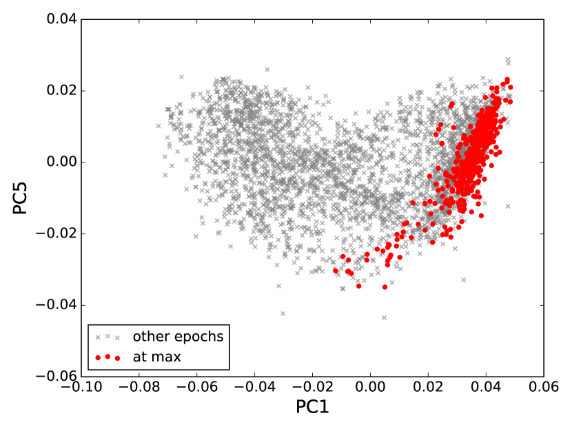
Figure 3: Distribution of spectra in the feature space formed by the 1^st and $5^{\boldsymbol{t}h}$ principal components. The red circles represent SN Ia spectra at maximum and the grey crosses denote SN Ia spectra in other epochs.

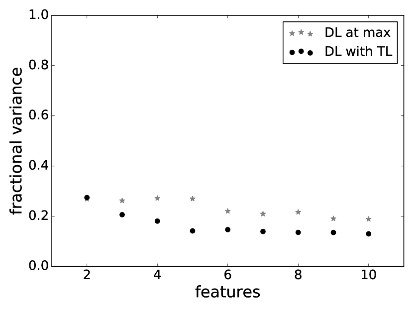
Figure 4: Variance between the deep learning reconstructions and observed SN Ia spectra at $B$ max. Gray crosses correspond to a data configuration using only SNe Ia at maximum (no transfer learning) and black circles denote results from an initial data matrix containing spectra from all epochs (with transfer learning). The horizontal axis stands for the number of features; the vertical axis shows the deviation between real data and reconstruction.

Our data scenario fits within the scope of transfer learning. One is given spectra from the same supernova at various epochs, which can be treated as different observations. Despite being the electromagnetic signature of different astrophysical conditions, spectra from different epochs share common properties (e.g., they all have absorption/emission lines). Consequently, if we consider each spectrum as an independent object (a different line in the data matrix) we can use all of them to train the deep learning network in recognizing spectral features.

Following this reasoning, our initial data matrix was built with all available SN Ia spectra, regardless of the epoch of the observation. This allows us to exploit all available spectra, even those with unknown epoch of observation, in the investigation of spectra properties at maximum. Closely related strategies, with different goals, were used by Richards et al. (2012) for semi-supervised photometric classification of SN curves, Vilalta et al. (2013) for cepheids classification and Kremer et al. (2015) for photometric redshift determination. Despite the increase in data volume, the resulting feature space is much more stable, less affected by the inclusion/removal of individual spectra, and provides a safer ground for spectral feature recognition. Thus, each line in our data matrix holds the derivative of the flux for an observed spectrum between $4000$ and $7000$Å, sampled in bins of 10Å. The complete matrix contains $3677$ lines and 300 columns and serves as input to the dimensionality reduction algorithm (Section 3).

Once the low dimensional space is determined, we select only those spectra of interest (within 3 days from maximum brightness, resulting in 486 individual spectra) for the unsupervised learning phase. Fig. 3 illustrates how the spectra around maximum occupy a well defined region in the principal component parameter space. This configuration can easily be used to study the time evolution of spectral features, as well as to estimate the epoch of a given spectrum. In this work, we focus on recognizing characteristics of SN Ia spectra at maximum.

In Fig. 4, we show how this approach impacts the reconstruction power of the DL feature space. The vertical axis represents residual variance between the reconstruction and the original data with (black circles) and without (grey stars) the transfer learning approach. To calculate variance, both data sets (one with all the spectra and another containing only spectra at B-maximum) were randomly split in a training ($80\%$) and a test set ($20\%$). DL was applied to both training sets with different number of features in the central layer. Resulting features were than used to reconstruct the spectra in the test set and the normalized residual variances between the predictions and the measured derivative spectra in the test set were then calculated. We observe that with transfer learning, 4 features suffice to converge to a stable fractional variance. Without transfer learning, the same performance level cannot be achieved, even if we employ 10 features along the intermediate layer.

5 Comparing feature spaces

In order to demonstrate how DL outperforms the standard PCA algorithm, we provide a detailed comparison between the two parameter spaces. Fig. LABEL:fig:rec_examples shows the reconstruction of the original spectra using PCA and DL. In black we show a few examples of SN Ia spectra at three representative epochs. The first four spectra are at ${\sim-13}$ days from $B$ max. Three spectra are close to $B$ max and, finally, three spectra are found in the nebular phase at ${\sim+180}$ days from maximum (from top left to bottom right).

Reconstructions using DL show very good agreement with observations at all epochs due to the non-linearity of its representations. It performs exceptionally well in the earliest and the latest spectra and on SNe with rare spectroscopic peculiarities such as, for example, SN 2005hk. The behaviour of the High Velocity Feature (Mazzali et al., 2005) of the Si ii 6355Å in the early spectra (for example SN 2002dj and SN 2002bo) are also finely reproduced by DL when compared to PCA. The latter is competitive only away from the early and late epochs, and on objects that are not too peculiar. For PCA to obtain reconstructions comparable to DL, we would need a large number of components. From this, it is clear that DL has an outstanding performance when compared to PCA, even when the latter uses almost 4 times the number of parameters.

Fig. 5 confirms this superiority quantitatively and, at the same time, highlights still another important advantage of the DL approach: the asymptotic behaviour of residual variances as the number of features increases. DL greatly outperforms PCA even when using a small number of features. Its reconstruction capability shows steady improvement until $\sim 5$ features, after that it remains approximately constant. PCA only achieves a comparable reconstruction with $\sim 15$ PCs. However, a large fraction of the variance explained by PCA can be traced to noise, and an unnecessary large number of components overfits the data (this is represented by the constant decrease in fractional variance as a function of the number of PCs). DL behaves robustly, less affected by noise, and preventing overfitting (the variance explained remains approximately constant for more than $\sim$4 features). This suggests that the intrinsic dimension in SN Ia spectra is $\sim 5$, leaving only $4$ hidden physical parameters to characterize the explosion (one of these dimensions is needed to explain the time evolution of the spectrum). Similar results concerning the number of significant parameters necessary to describe the spectral features of SN Ia were reported by Sasdelli et al. (2015). This hints to the apparent simplicity of the space of SN Ia spectra and should be considered in model development process.

Once we have demonstrated the superiority of DL in reducing the dimensionality of the parameter space we move to the visualization and unsupervised clustering steps. In what follows, all analyses where performed on the 4 dimensional DL feature space.

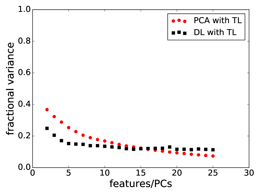
Figure 5: Comparison between Deep Learning and PCA in their capacity to reconstruct the original spectra and robustness to overfitting. Horizontal axis stands for the number of PCs/features and vertical axis shows the deviation between real data and reconstruction.

6 Data visualization

Given that DL is a relatively new technology in machine learning, and has no precedence in the study of SN Ia spectra, we provide the reader with a couple of visualization tools to enable analysis of this feature space. The two algorithms described below are part of the field of dimensionality reduction, but here we employ them as visualization tools.

6.1 Self-organizing maps

Self-Organizing Maps (SOM) are a special kind of artificial neural networks, often invoked to visualize data in an unsupervised manner. They are commonly used to find a two-dimensional embedding of the data and have been extensively employed in astronomy, e.g., in stellar spectra (Mahdi, 2011), light curve classification (Brett et al., 2004), and object selection and photometric redshift estimation (Way & Klose, 2012; Geach, 2012).

The main idea behind SOM is to construct a 2-dimensional representation of the data where similar objects are placed close to each other. The algorithm can be described as follows: consider data in $\mathbb{R}^{d}$, and a two-dimensional grid $M=S_{1}\times S_{2}$. Initially each cell of the grid, $C\in M$, hosts a random vector $\mathbf{c}\in\mathbb{R}^{d}$, called prototype (these are initially random, they iteratively become more representative of the data vectors assigned to their cell). One then chooses, at random, one element from the data set, $\mathbf{x}\in\mathbb{R}^{d}$, and compares it to all prototypes in the grid using, for example, the Euclidean distance in $\mathbb{R}^{d}$. Let $\mathbf{p}$ be the prototype in the grid that is closest to $\mathbf{x}_{i}$ and $P\in M$ denote the grid cell hosting $\mathbf{p}$. Subsequently, $\mathbf{p}$ and all prototypes $\mathbf{q}$ of neighbouring cells $Q$ of $P$ are updated according to the following rule:

$$\mathbf{q}=\mathbf{q}+\alpha\cdot h(P,Q)\cdot(\mathbf{x}-\mathbf{p}),$$ (5)

where $h$ is a neighbourhood function (typical functions are $h\equiv 1$, $h(P,Q)=\left\lVert P-Q\right\rVert$, or $h(P,Q)=e^{-{(\sqrt{2}\sigma)}^{-2}\left\lVert P-Q\right\rVert^{2}}$) and $\alpha$, named learning rate, is usually reduced during the iterative process. Thus, prototypes of $P$ and its neighbouring cells are made “more similar” to $\mathbf{x}$. Another element from the data set, $\mathbf{x}$', is then compared to this new grid configuration. If this data vector is very similar to the first, it is allocated in $P$ or one of its neighbouring cells. Otherwise, it will populate another cell, $P$', defining a new locus on the grid which will host its characteristics. The comparison is repeated for all objects in the data and for the entire data set until convergence. As a result, we are left with a 2-dimensional re-organization of the initial data, where similar objects are allocated in nearby cells, and distinct ones occupy different extremes of the grid.

Fig. 6 shows results after applying SOM to the 4-dimensional DL feature space. As described in Section 4, in this task we select only spectra close to maximum. The grid contains 10$\times$10 individual cells showing the mean spectra (black line), standard deviations (pink/purple), the numbers of spectra allocated in each individual cell and the sub-type of the majority of objects in each cell (when the cell population is exactly split between subtypes both labels are shown). We emphasize that Fig. 6 does not show the final prototypes in each cell, but the mean of all the spectra allocated in them. We chose this visualization because the prototypes in our case would relate to the 4-dimensional DL space, making it impossible to recognize spectral features. Different spectroscopic classes are arranged over different parts of the grid. Normal SNe Ia such as SN 1994D and SN 2011fe are close to the centre of the grid, the peculiar and faint 91bg-like cluster on the top left and the high velocity SNe are on the bottom left corner. We also recognize 91T-like SNe on the right side of the grid. From this configuration, we can already tell that the DL feature space is able to grasp crucial differences between different spectral features. Literature suggests that 91T-like, High Velocity and 91bg-like SNe are the extremes of SN Ia spectral variability, while 91bg-like SNe are possibly a more isolated group (Cormier & Davis, 2011; Blondin et al., 2012). In this context, spectroscopically normal SNe Ia form the bulk of the data set, connecting the other subtypes together through an almost continuous change in spectral features. These findings are nicely confirmed by our SOM analysis, which gives us a glimpse of the potential of this feature space. In the following sections, we show how this first visual analysis is in concordance with the more quantitative results obtained using unsupervised learning.

Figure 6: A self organized map of SN Ia spectra at maximum, constructed from the Deep Learning 4-dimensional feature space. Black lines correspond to the mean spectra of each cell, purple and blue bands correspond $1\sigma$ and $2\sigma$ respectively. Also shown are the number of spectra allocated in each individual cell and the subtype of the majority of SNe populating each cell according to the classification proposed by Wang et al. (2009b). In case there are exactly the same number of objects of different subtypes both labels are shown.

6.2 Isomap

Isomap belongs to a broader class of dimensionality reduction techniques known as manifold learning. While PCA seeks to preserve the variance of the data, Isomap preserves its intrinsic geometry (Tenenbaum et al., 2000). More precisely, it can be seen as an extension of another classical dimensionality reduction method, called multi-dimensional scaling (MDS), which aims at finding a low-dimensional embedding of the data, such that the distance between any pair of two points is preserved. Isomap generalizes this idea by resorting to “geodesic manifold distances”, which are approximated via, e.g., a neighbourhood graph in which two points (nodes) are connected if one of the points is within the set of the $K$-nearest neighbours of the other one (Tenenbaum et al., 2000). The geodesic distance, $d_{M}(i,j)$, between two points $i$ and $j$ can be defined as the shortest path between the two points in that graph. These distances are then used as in classical MDS, which usually resorts to the standard Euclidean distance (“straight lines”). Thus, in contrast to MDS, Isomap can also capture non-linear manifold structures. In astronomy, it was recently applied to spectroscopic classification by Bu et al. (2014).

In what follows, we use Isomap to provide a 2-dimensional visualization of the 4-dimensional feature space obtained with DL. It provides a much clearer view of the distribution of points in the DL feature space and facilitates a visual comparison with other classifications schemes.

7 Unsupervised learning

In previous sections we introduced efficient dimensionality reduction techniques. We now turn to the last step of our endeavour: unsupervised learning. Our main goal is to show the feasibility of automatically identifying subtypes of SNe Ia with minimum assumptions about the physics and dynamics of the SN mechanism. Unsupervised learning techniques identify clusters in a data set by maximizing the similarity among objects within the same cluster, and maximizing the dissimilarity among objects from different clusters.

The computational complexity of a clustering algorithm increases as the dimension of the data grows larger. This is because added dimensions quickly increase the volume of the feature space and the data becomes sparse; the capacity of finding clusters then deteriorates. This effect is known as the curse of dimensionality. DL represents our solution to mitigate this effect.

While there are many clustering algorithms readily available, K-Means is certainly the most popular. We have compared different methods using simulated data and found K-Means to exhibit good performance. We focus on this method in the following sections.

7.1 K-means

The K-means algorithm is one of the most well-known clustering techniques, yielding intuitive solutions. In its original form (MacQueen, 1967) it begins by choosing at random $k$ vectors of the same dimensions of the data (with $k$ chosen by the user). These will act as centres for potential clusters definition. A distance (Euclidean) is then calculated between all vectors in the data set and the centre candidates. Each data point is assigned to the cluster represented by its closest centre candidate. Once the first set of clusters is defined, the centre candidates are updated to the centroid defined by all the members in each cluster. The process is repeated until the centroids are not changed due to further iterations. In practice, this local search strategy quickly converges to a solution (e.g., after 50 iterations).

One drawback of K-means is the need to explicitly state the number of clusters a priori. In our case, we wish to show that our approach is able to grasp the main spectral features underlying the classification proposed by Wang et al. (2009b) (which is composed by subtypes normal, high-velocity, 91T-like and 91bg-like) and, as a consequence, we will search for up to 4 clusters. A deeper analysis quantifying the degree of cluster coherence throughout different number of clusters will be addressed in a subsequent paper.

All the methods described above have been made available in a single toolbox that enables quick analysis of a (potentially) large initial data set. We present DRACULA (Dimensionality Reduction And Clustering for Unsupervised Learning in Astronomy) in detail in appendix B.

8 Results

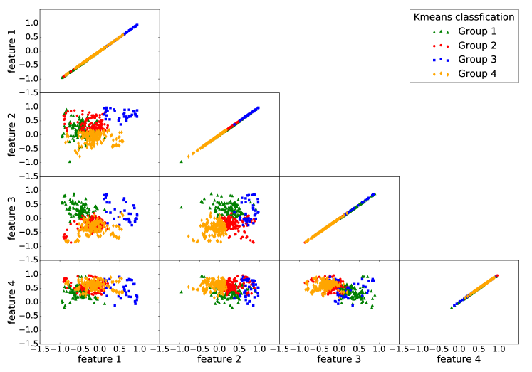
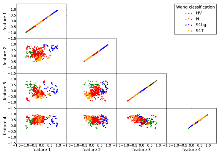
Figure 7: Four dimensional feature space resulting from Deep Learning. Each point corresponds to one SN Ia spectrum within $-3$ and $+3$ days since $B$-maximum. Top: Colours represent the groups found by the K-Means algorithm when 4 groups are required. Bottom: Colours correspond to the classification suggested by Wang et al. (2009b). This plot does not show the objects classified as “peculiar”.

We used DRACULA to analyse the sample of SN Ia spectra introduced in Section 2. Results shown below correspond to the 4-dimensional DL feature space (Section 5) ran through the K-Means algorithm. In order to compare our results with the classification proposed by Wang et al. (2009b), we set K-Means to search for 4 distinct clusters (Section 7).

Fig. 7 shows the 4-dimensional DL feature space configuration. In the upper panel, colours correspond to the clusters found by K-Means; in the lower panel points are identified according to Wang et al. (2009b) classification (the lower panel of Fig. 7 does not show the SNe classified as “peculiar” by Wang et al. (2009b) because there is not a unique underlying spectral characteristic which defines this group). Although the two classification schemes are not in complete agreement, they share some basic characteristics. For example, the scatter plot in the feature space formed by features 1 and 2 are quite similar in the upper and lower panels, indicating the correspondence between group 3 (upper panel) and 1991bg-like SNe (lower panel).

A better visualization of this feature space is achieved by applying the isomap algorithm (Section 6.2) to the 4-dimensional DL feature space. Fig. 9 shows the resulting 2-dimensional isomap space with the clusters found by K-Means (left panel) and the SN Ia subtypes defined by Wang et al. (2009b, right panel). The spectra of a few SNe located at the transition between two subclasses are highlighted. This figure not only demonstrates how isomaps can be a powerful tool in high dimensional data visualization, but also clarifies the potential of combining DL with unsupervised learning algorithms. Moreover, it confirms that currently defined SNe Ia subtypes are extremes of a continuous distribution of spectral features. Many of the SNe located between different classes have been recognized as peculiar (e.g. SN 2006bt Foley et al., 2010), or “unusual” (SN 1999ac Garavini et al., 2005) objects, and the classification of SN 1999ac as a 91T-like is at least dubious (Phillips et al., 2006). Peculiar characteristics, like a blue $B-V$ colour typical of 91T-like objects, are recognized even in the cases where these transitional objects were classified as normal (e.g. SN 1998aq Branch et al., 2003b). This is a clear evidence of the existence of intermediary objects in the frontiers of SNe Ia subclasses and the consequent continuum characteristics of its spectral features space.

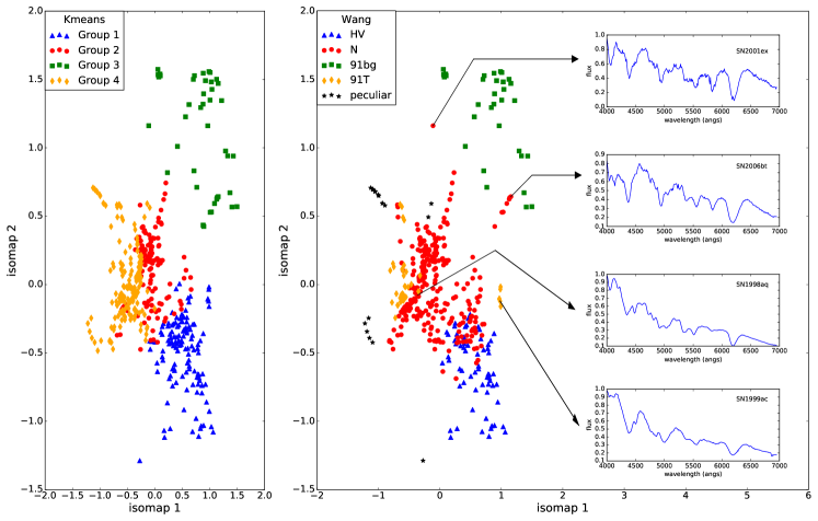
Figure 8: Four dimensional feature space from Deep Learning reduced to 2 dimensions through isomap. Left: Groups found by the K-Means algorithm when 4 groups are imposed. Right: Objects separated according to the classification proposed by Wang et al. (2009b). In this panel we also highlight spectra of 4 SNe lying in the boundary between classes.

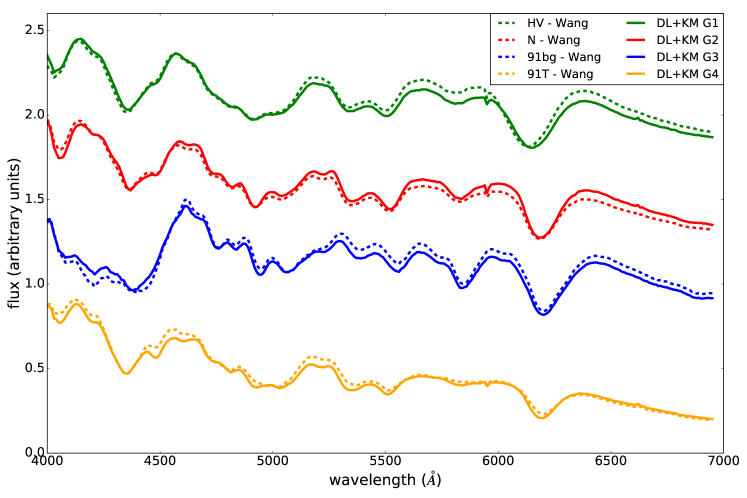
Figure 9: Comparison between the mean spectrum found by Deep Learning + K-Means (full lines) and mean spectrum of the SNe Ia subtypes defined by Wang et al. (2009b, dashed lines).

Our goal is to identify which spectral characteristics correspond to the extremes. Fig. 9 shows the mean spectrum of each cluster in both classification schemes. The agreement between the mean spectra is proof that DL, when coupled with unsupervised learning algorithms, is able to automatically identify important spectral features without human screening. The method recovers classes similar to those defined by visual inspection; this can be used to optimize the current identification of types or subtypes of SNe.

Our methodology is also capable of identifying a hierarchical structure within the data set. Fig. LABEL:fig:KMeans1234 shows the mean spectrum of all SN Ia spectra at maximum (top-left panel) as well as the mean spectrum of each cluster found by K-Means using $k=2$ to $k=4$ clusters, comparing it with the mean spectra of subtypes proposed by Wang et al. (2009b). Given the data set at hand, we see that the velocity at which most lines form (the velocity of the photosphere) is the first order spectral characteristic which defines subtypes of SNe Ia (2-cluster configuration). After this, 1991bg-like objects are kept in a cluster of their own (3-cluster configuration) and finally 91T-like objects are separated. Depending on the degree of specialization we demand from the data, we are able to recognize a sequence of spectral features which might be used to guide the physical basis of future data-driven classification systems.

Our analysis suggests that the currently defined SN Ia subtypes are extremes of a continuous distribution of spectral features and that SNe Ia live in a small multi-dimensional continuum with no strict boundaries separating subclasses and likely governed by few key physical parameters.

9 Summary and Discussion

We propose a framework to automatically identify subtypes of SNe Ia within a set of measured spectra by combining modern machine learning techniques. As a first application of this tool, we investigate how to recover previously reported subtypes of SNe Ia.

The set of public SN Ia spectra (Section 2) was first submitted to the preprocessing described in Sasdelli et al. (2015) and the resulting matrix was used as input for the algorithm which can be summarized in 3 main steps: transfer learning, dimensionality reduction, and unsupervised learning.

The goal of transfer learning is to ensure the stability of the low dimensional feature space by adding a large variety of spectra in the original data matrix. In our example, although the clustering analysis is focused at B-maximum, we use spectra from all available epochs for training. Once the low dimensional feature space is constructed, only the projections corresponding to spectra at maximum are selected for the next phase (figure 3).

We introduce Deep Learning for dimensionality reduction on SN Ia spectra. This is a cutting-edge technique only recently introduced to astronomy (Huertas-Company et al., 2015). We prove its effectiveness in spectroscopy data analysis and show that it outperforms the PCA algorithm in the reconstruction of measured spectra, reducing the dimensionality of the feature space from $\sim 300$ hundreds to 4. Since this is the first application of Deep Learning for SN Ia spectra characterization, we use Self- Organizing Maps (SOM) to better understand the potential of the new reduced feature space (figure 6); this visualization technique shows how spectral properties vary in the SN Ia spectra space; specifically it allows the visualization of the peculiarity of subtypes reported in the literature, e.g., the 91bg-like SNe (Cormier & Davis, 2011; Blondin et al., 2012).

Lastly, we use unsupervised learning techniques to investigate the possibility of identifying spectroscopic features in subclasses of SN Ia spectra at maximum light. This allows us to define a data-driven classification scheme a posteriori and analyse clusters separately in order to look for their spectroscopic characteristics. This facilitates the classification of a fairly large data set requiring the astronomer to visually inspect only a handful of possibilities (the mean spectra). We use the low dimensional space from Deep Learning as an input for the K-Means algorithm. In order to provide a more friendly visualization of the four dimensional feature space, we use isomap as a further layer of dimensionality reduction. Here the separation between the clusters is more evident; the identification with the Wang et al. (2009b) clusters is also clearer.

We find that the spectral variability of SNe Ia can be summarized by a low dimensional space. Spectra starting from few days from the explosion up to more than a year afterwards can be parametrized by a 5-dimensional space. The time evolution of the spectra uses one of these dimensions. This result suggests that only 4 underlying physical parameters suffice to describe SN Ia explosions and their spectroscopic variability, including the most “peculiar” objects, such as 91bg-like and the 02cx-like SNe.

SNe Ia are well known as a uniform class of objects. Our results prove this claim, and suggest that progenitors should be a “simple” system with no more than a handful of initial parameters. Moreover, we also show that the currently identified SN Ia sub-types are in fact the extremes of a continuous distribution of spectral features. We also do not find strong evidences of distinct subclasses.

Our complete software apparatus was built under DRACULA, a publicly available Python package that is here tested on a public data set of SN Ia spectra. Our results show agreement between mean cluster spectra and those proposed by Wang et al. (2009b). Our method is also able to identify a hierarchical structure within the data set, confirming previous statements that high velocity features are of the first order effect in separating currently available samples of SNe Ia (Wang et al., 2013). Future work considers analysis of time evolution in SN Ia spectra, and the possibility of using our tool in the classification of other supernova types.

Appendix A Glossary

To avoid confusion due to different nomenclatures used by the machine learning and astronomy communities, we provide a list of the terms used in this paper:

• Class/subclass (Supernova Physics): these denote different underlying physical models or characteristics of the progenitor system.

• Feature (Machine Learning): a recorded property or observation. In our context it corresponds to the flux (or the derivative of the flux) of a given wavelength bin.

• Feature space (Machine Learning): commonly known in astronomy as parameter space. This space is originally of high dimensionality ($\sim 300$ wavelength bins), but is reduced to a 4-dimensional space when we invoke Deep Learning.

• Parameter (Computing): an input variable of a computer algorithm.

• Physical parameter (Supernova Physics): a generic term to describe one of the initial conditions of the supernova explosion.

• Prototype (SOM): vectors populating each cell of a SOM grid. Initially random, they iteratively become more representative of the data vectors assigned to their cell.

• Spectral feature (Spectroscopy): absorption and/or emission feature in the spectrum. It originates from a group of atomic lines with similar energy. It is usually dominated by the lines of a single ion.

• Type/subtype (Supernova Physics): these denote different categories of SNe based on spectral features (e.g. HV, 91T-like, etc.).

• Weight parameter (Deep Learning): weight matrices connecting adjacent layers of the Deep Learning network. Weights are optimized during the training phase using the training sample.

Appendix B DRACULA

We present DRACULA (Dimensionality Reduction And Clustering for Unsupervised Learning in Astronomy), an implementation of the methods discussed in this paper. The toolbox is written in Python, is publicly available, and can be easily adapted to multiple applications. The software relies heavily on tools developed in scikit-learn (Pedregosa et al., 2011). The DL analysis used the H2O package (Arora et al., 2015) and the SOM routine used the Kajić et al. (2014) implementation. Thanks to its modular design, all main steps, e.g., dimensionality reduction, unsupervised learning (clustering) and plotting, can be run separately. A flowchart illustrating the code capabilities is shown in Fig. LABEL:fig:flowchart.

In what follows, we demonstrate how DRACULA can be invoked to obtain similar results to those presented in this paper. We avoid a detailed description of all code functionalities, and focus on main procedures (the documentation provides more detailed descriptions). Let us start assuming an initially big data matrix. In our case, this is composed of derivatives over the flux logarithm, as described in Section 2. We now go through each step described in previous sections and demonstrate how the user can reproduce our results using DRACULA.

B.1 Dimensionality Reduction

To begin, the user needs to set up a configuration file (which must be named config.py) to define the type of desired analysis. This module contains four methods: PCA (Jolliffe, 1986), Expectation Maximization PCA (Bailey, 2012), Kernel PCA (Schölkopf et al., 1999) and DL (Deng & Yu, 2014). Dimensionality reduction requires as input a list of observed features for each object (1 line per object, 1 column per feature). For clarity, input and output are defined next:

• input: data amenable to reduction (ex: spectra derivatives)

• output: reduced data

In order to perform dimensionality reduction with DL the configuration file must contain the keywords: ORG_DATA, that receives the path to the file with uncompressed data and REDUCTION_METHOD that determines the dimensionality reduction algorithm. If no other options are included in the configuration file, the code will run using default values. The user might change default values by modifying the random seed, DeepLearning_seed, number and structure of hidden layers, DeepLearning_n_layers and DeepLearning_hidden respectively, in the configuration file.

One can run the chosen dimensionality reduction routine from the command line typing DRAC_REDUCTION. The output containing the reduced data is created in a folder called red_data.

B.2 Clustering

Clustering follows using the output file from the last section or using an externally reduced dataset. In the case of an external source, ORG_DATA should be commented out and the path to the externally reduced file must be given as

⬇

1REDUCED_DATA_EXTERNAL = "<path to reduced data>"

The running format is the same as dimensionality reduction, where the input is the reduced data. After clusters are detected, the algorithm outputs their centres and the corresponding labels for each object. In short:

• input: reduced data

• output: centers of clusters and labels for each object in the reduced data file

Available options here are KMeans (MacQueen, 1967; Arthur & Vassilvitskii, 2007), Mean Shift (Comaniciu & Meer, 2002), Agglomerative Clustering (Voorhees, 1986), Affinity Propagation (Comaniciu & Meer, 2002) and DBSCAN (Ester et al., 1996). For our particular case, the configuration file contains:

⬇

1CLUSTERING_METHOD = "KMeans"

Analogous to the dimensionality reduction case, the user can change parameters. An example is the number of clusters, using variable KMeans_n_clusters. The default value is KMeans_n_clusters=4. At this stage it is also possible to use a mask, which is specially important for cases where transfer learning is applied (e.g., when the dimensionality reduction algorithm is applied to a big diverse matrix and only a subset of the reduced data is intended for clustering). The mask consists of a file with the same number of lines as the reduced data; in each line “1” indicates objects included in the clustering analysis and “0” refers to all remaining objects. The path for the mask should be provided as follows:

⬇

1MASK_DATA = ’<path to mask file>’

The clustering routines can be run in the command line by typing DRAC_CLUSTERING.

B.3 Varying parameters

In cases where it is necessary to compare the output from a range of parameters, DRACULA allows the user do it automatically, however, beware that this functionality only permits to change one parameter at a time. The parameters to be declared in the configuration file are

⬇

1VAR_TYPE = ’CLUSTERING’ or ’REDUCTION’

2VAR_PAR = ’REDUCTION_METHOD’ or ’CLUSTERING_METHOD’

3VAR_VALS = [1,2,3] or [’name1’,’name2’,’name2’] or [vec1,vec2,vec3]

This functionality uses the same configuration file (config.py) with the above extra keys, and can be run by typing DRAC_COMPARISON.

B.4 Plotting

It is useful to plot results to gain insight on the cluster quality. Plots can be generated for the whole process, from reduction to clustering, with input and output given by:

• input: reduced data, cluster centres and labels for each object in the reduced data file

• output: scatter plot of reduced data coloured according to labels

Scatter plots, similar to those shown in Fig. 7, are generated by typing DRAC_PLOT. The format of the output files is selected by setting the keyword PLOT_EXT, in the configuration file.

If one wishes to use this tool for plotting clusters assigned by an external clustering algorithm, the path to the corresponding labels should be provided:

⬇

1LABELS_DATA_EXTERNAL = "<path to labels file>"

Finally, it is useful to visualize the mean input data within each cluster so features can be compared with expected patterns. The interface in this case is

• input: reduced data and cluster labels

• output: plot of mean input data for each cluster

If the data for visualization is not in the file used to make the reduction (in our case the reduction is performed on the derivative of the spectra, but we would like to observe the mean spectrum of each group found by K-Means), it can be plotted by setting:

⬇

1SPECTRAL_DATA_EXTERNAL = "<path to original data file>"

The format of the output file for the mean data (or mean spectrum) needs to be set separately through the keyword PLOT_SPEC_EXT. The plots can be generated using the command DRAC_PLOT_SPECS.

We emphasize that the above provides only a glimpse of the capabilities of DRACULA. The package has other functionalities (e.g. cluster validation routines) which will be fully explored, and described, in subsequent work.

B.5 SOM

The SOM module (Section 6.1) is independent from the steps previously described. The interface is as follows:

• input: reduced data

• output: SOM grid

This module requires its own configuration file, which must be called config_som.py. The path to the reduced data file is given through the keyword ORG_DATA. When no other option is provided in the configuration file, the module will run a $10\times 10$ matrix through 100 iterations, and the output plot will show the prototypes populating each cell. If the user wants the SOM grid to show the mean of the original data (in our case, the mean of observed spectra assigned to each cell), the keyword SPECTRAL_DATA_EXTERNAL must point to the original data file. The number of iterations can be set by adding the keyword Niter to the configuration file. The grid shown in Fig. 6 was constructed with Niter = 10000000. SOM module can be run by typing DRAC_SOM.

References

- Altavilla et al. (2007) Altavilla G., et al., 2007, A&A, 475, 585
- Anupama et al. (2005) Anupama G. C., Sahu D. K., Jose J., 2005, A&A, 429, 667
- Arora et al. (2015) Arora A., Candel A., Lanford J., LeDell E., Parmar V., 2015, Deep Learning with H2O. http://h2o.ai/resources
- Arsenijevic (2011) Arsenijevic V., 2011, MNRAS, 414, 1617
- Arthur & Vassilvitskii (2007) Arthur D., Vassilvitskii S., 2007, in Proceedings of the Eighteenth Annual ACM-SIAM Symposium on Discrete Algorithms. SODA ’07. Society for Industrial and Applied Mathematics, Philadelphia, PA, USA, pp 1027–1035, http://dl.acm.org/citation.cfm?id=1283383.1283494
- Bailey (2012) Bailey S., 2012, PASP, 124, 1015
- Ball & Brunner (2010) Ball N. M., Brunner R. J., 2010, International Journal of Modern Physics D, 19, 1049
- Barbon et al. (1990) Barbon R., Benetti S., Rosino L., Cappellaro E., Turatto M., 1990, A&A, 237, 79
- Benetti et al. (2004) Benetti S., et al., 2004, MNRAS, 348, 261
- Benetti et al. (2005) Benetti S., et al., 2005, ApJ, 623, 1011
- Bengio et al. (2013) Bengio Y., Courville A., Vincent P., 2013, IEEE Transactions on Pattern Analysis and Machine Intelligence, 35, 1798
- Benitez-Herrera et al. (2013) Benitez-Herrera S., Ishida E. E. O., Maturi M., Hillebrandt W., Bartelmann M., Röpke F., 2013, MNRAS, 436, 854
- Blondin et al. (2012) Blondin S., et al., 2012, AJ, 143, 126
- Branch et al. (2003a) Branch D., et al., 2003a, AJ, 126, 1489
- Branch et al. (2003b) Branch D., et al., 2003b, AJ, 126, 1489
- Branch et al. (2009) Branch D., Dang L. C., Baron E., 2009, PASP, 121, 238
- Brett et al. (2004) Brett D. R., West R. G., Wheatley P. J., 2004, Monthly Notices of the Royal Astronomical Society, 353, 369
- Bu et al. (2014) Bu Y., Chen F., Pan J., 2014, New Astronomy, 28, 35
- Bufano et al. (2009) Bufano F., et al., 2009, ApJ, 700, 1456
- Cappellaro et al. (2001) Cappellaro E., et al., 2001, ApJ, 549, L215
- Chornock et al. (2006) Chornock R., Filippenko A. V., Branch D., Foley R. J., Jha S., Li W., 2006, PASP, 118, 722
- Comaniciu & Meer (2002) Comaniciu D., Meer P., 2002, Pattern Analysis and Machine Intelligence, IEEE Transactions on, 24, 603
- Cormier & Davis (2011) Cormier D., Davis T. M., 2011, MNRAS, 410, 2137
- Crisci et al. (2012) Crisci C., Ghattas B., Perera G., 2012, Ecological Modelling, 240, 113
- De Souza et al. (2014a) De Souza R. S., Maio U., Biffi V., Ciardi B., 2014a, MNRAS, 440, 240
- De Souza et al. (2014b) De Souza R. S., Ishida E. E. O., Whalen D. J., Johnson J. L., Ferrara A., 2014b, MNRAS, 442, 1640
- Deng & Yu (2014) Deng L., Yu D., 2014, Found. Trends Signal Process., 7, 197
- Elias-Rosa et al. (2006) Elias-Rosa N., et al., 2006, MNRAS, 369, 1880
- Ester et al. (1996) Ester M., Kriegel H.-P., Sander J., Xu X., 1996, in Proc. of 2nd International Conference on Knowledge Discovery and. pp 226–231
- Ferreras et al. (2006) Ferreras I., Pasquali A., de Carvalho R. R., de la Rosa I. G., Lahav O., 2006, MNRAS, 370, 828
- Folatelli et al. (2013) Folatelli G., et al., 2013, ApJ, 773, 53
- Foley et al. (2010) Foley R. J., Narayan G., Challis P. J., Filippenko A. V., Kirshner R. P., Silverman J. M., Steele T. N., 2010, ApJ, 708, 1748
- Garavini et al. (2004) Garavini G., et al., 2004, AJ, 128, 387
- Garavini et al. (2005) Garavini G., et al., 2005, AJ, 130, 2278
- Garavini et al. (2007) Garavini G., et al., 2007, A&A, 471, 527
- Geach (2012) Geach J. E., 2012, MNRAS, 419, 2633
- Gerardy (2005) Gerardy C. L., 2005, in Turatto M., Benetti S., Zampieri L., Shea W., eds, Astronomical Society of the Pacific Conference Series Vol. 342, 1604-2004: Supernovae as Cosmological Lighthouses. p. 250
- Gerardy et al. (2007) Gerardy C. L., Meikle W. P. S., Kotak R., Höflich P., Farrah D., Filippenko A. V., Foley R. J., et al. 2007, ApJ, 661, 995
- Gómez & López (1998) Gómez G., López R., 1998, AJ, 115, 1096
- Graur & Maoz (2013) Graur O., Maoz D., 2013, MNRAS, 430, 1746
- Hachinger et al. (2006) Hachinger S., Mazzali P. A., Benetti S., 2006, MNRAS, 370, 299
- Hamuy et al. (2002) Hamuy M., et al., 2002, AJ, 124, 417
- Hicken et al. (2007) Hicken M., Garnavich P. M., Prieto J. L., Blondin S., DePoy D. L., Kirshner R. P., Parrent J., 2007, ApJ, 669, L17
- Hillebrandt et al. (2013) Hillebrandt W., Kromer M., Röpke F. K., Ruiter A. J., 2013, Frontiers of Physics, 8, 116
- Hinton & Salakhutdinov (2006) Hinton G. E., Salakhutdinov R. R., 2006, Science, 313, 504
- Huertas-Company et al. (2015) Huertas-Company M., et al., 2015, ApJS, 221, 8
- Ishida & de Souza (2011) Ishida E. E. O., de Souza R. S., 2011, A&A, 527, A49
- Ishida & de Souza (2013) Ishida E. E. O., de Souza R. S., 2013, MNRAS, 430, 509
- Ishida et al. (2011) Ishida E. E. O., de Souza R. S., Ferrara A., 2011, MNRAS, 418, 500
- Ivezic et al. (2014) Ivezic Z., Connolly A. J., VanderPlas J. T., Gray A., 2014, Statistics, Data Mining, and Machine Learning in Astronomy: A Practical Python Guide for the Analysis of Survey Data, stu - student edition edn. Princeton University Press, http://www.jstor.org/stable/j.ctt4cgbdj
- Jha et al. (1999) Jha S., Garnavich P., Challis P., Kirshner R., Berlind P., 1999, IAU Circ., 7149
- Jolliffe (1986) Jolliffe I., 1986, Principal Component Analysis. Springer Verlag
- Kajić et al. (2014) Kajić I., Schillaci G., Bodiroža S., Hafner V. V., 2014, in Proceedings of the 2014 ACM/IEEE International Conference on Human-robot Interaction. HRI ’14. ACM, New York, NY, USA, pp 192–193, doi:10.1145/2559636.2559816, http://doi.acm.org/10.1145/2559636.2559816
- Kotak et al. (2005) Kotak R., et al., 2005, A&A, 436, 1021
- Kremer et al. (2015) Kremer J., Gieseke F., Steenstrup Pedersen K., Igel C., 2015, Astronomy and Computing, 12, 67
- Krisciunas et al. (2007) Krisciunas K., et al., 2007, AJ, 133, 58
- Krone-Martins et al. (2014) Krone-Martins A., Ishida E. E. O., de Souza R. S., 2014, MNRAS, 443, L34
- LeCun et al. (2015) LeCun Y., Bengio Y., Hinton G., 2015, Nature, 521, 436
- Leonard (2007) Leonard D. C., 2007, in Immler S., Weiler K., McCray R., eds, American Institute of Physics Conference Series Vol. 937, Supernova 1987A: 20 Years After: Supernovae and Gamma-Ray Bursters. pp 311–315, doi:10.1063/1.3682922
- Li et al. (1999) Li W. D., et al., 1999, AJ, 117, 2709
- Li et al. (2001a) Li W., et al., 2001a, PASP, 113, 1178
- Li et al. (2001b) Li W., Filippenko A. V., Treffers R. R., Riess A. G., Hu J., Qiu Y., 2001b, ApJ, 546, 734
- Libbrecht & Noble (2015) Libbrecht M. W., Noble W. S., 2015, Nat Rev Genet, 16, 321
- MacQueen (1967) MacQueen J. B., 1967, in Proceedings of 5th Berkeley Symposium on Mathematical Statistics and Probability. pp 281–297
- Madgwick et al. (2003) Madgwick D. S., Hewett P. C., Mortlock D. J., Wang L., 2003, ApJ, 599, L33
- Mahdi (2011) Mahdi B., 2011, preprint, (arXiv:1108.0514)
- Matheson et al. (2008) Matheson T., et al., 2008, AJ, 135, 1598
- Mazzali et al. (1995) Mazzali P. A., Danziger I. J., Turatto M., 1995, A&A, 297, 509
- Mazzali et al. (2005) Mazzali P. A., et al., 2005, ApJ, 623, L37
- Mitra et al. (2011) Mitra S., Choudhury T. R., Ferrara A., 2011, MNRAS, 413, 1569
- Morrey (1968) Morrey J. R., 1968, Analytical Chemistry, 40, 905
- Nugent et al. (1995) Nugent P., Phillips M., Baron E., Branch D., Hauschildt P., 1995, ApJ, 455, L147
- Pan & Yang (2010) Pan S. J., Yang Q., 2010, IEEE Trans. on Knowl. and Data Eng., 22, 1345
- Pastorello et al. (2007) Pastorello A., et al., 2007, MNRAS, 377, 1531
- Patat et al. (1996) Patat F., Benetti S., Cappellaro E., Danziger I. J., della Valle M., Mazzali P. A., Turatto M., 1996, MNRAS, 278, 111
- Paykari et al. (2014) Paykari P., Lanusse F., Starck J.-L., Sureau F., Bobin J., 2014, A&A, 566, A77
- Pedregosa et al. (2011) Pedregosa F., et al., 2011, Journal of Machine Learning Research, 12, 2825
- Perlmutter et al. (1999) Perlmutter S., et al., 1999, ApJ, 517, 565
- Phillips et al. (2006) Phillips M. M., et al., 2006, AJ, 131, 2615
- Phillips et al. (2007) Phillips M. M., et al., 2007, PASP, 119, 360
- Pignata et al. (2008) Pignata G., et al., 2008, MNRAS, 388, 971
- Quionero-Candela et al. (2009) Quionero-Candela J., Sugiyama M., Schwaighofer A., Lawrence N. D., 2009, Dataset Shift in Machine Learning. The MIT Press
- Richards et al. (2012) Richards J. W., Homrighausen D., Freeman P. E., Schafer C. M., Poznanski D., 2012, MNRAS, 419, 1121
- Riess et al. (1998) Riess A. G., et al., 1998, AJ, 116, 1009
- Salvo et al. (2001) Salvo M. E., Cappellaro E., Mazzali P. A., Benetti S., Danziger I. J., Patat F., Turatto M., 2001, MNRAS, 321, 254
- Sasdelli et al. (2015) Sasdelli M., et al., 2015, MNRAS, 447, 1247
- Sasdelli et al. (2016) Sasdelli M., Ishida E. E. O., Hillebrandt W., Ashall C., Mazzali P. A., Prentice S., 2016, MNRAS,
- Schölkopf et al. (1999) Schölkopf B., Smola A. J., Müller K.-R., 1999, MIT Press, Cambridge, MA, USA, Chapt. Kernel Principal Component Analysis, pp 327–352, http://dl.acm.org/citation.cfm?id=299094.299113
- Silverman et al. (2012) Silverman J. M., et al., 2012, MNRAS, 425, 1789
- Stanishev et al. (2007) Stanishev V., et al., 2007, A&A, 469, 645
- Taubenberger et al. (2008) Taubenberger S., et al., 2008, MNRAS, 385, 75
- Tenenbaum et al. (2000) Tenenbaum J. B., Silva V. d., Langford J. C., 2000, Science, 290, 2319
- Turatto et al. (1996) Turatto M., Benetti S., Cappellaro E., Danziger I. J., Della Valle M., Gouiffes C., Mazzali P. A., Patat F., 1996, MNRAS, 283, 1
- Turatto et al. (1998) Turatto M., Piemonte A., Benetti S., Cappellaro E., Mazzali P. A., Danziger I. J., Patat F., 1998, AJ, 116, 2431
- Valentini et al. (2003) Valentini G., et al., 2003, ApJ, 595, 779
- Vidyasagar (2015) Vidyasagar M., 2015, Annual Review of Pharmacology and Toxicology, 55, 15
- Vilalta et al. (2013) Vilalta R., Gupta K. D., Macri L., 2013, Astronomy and Computing, 2, 46
- Vincent et al. (2008) Vincent P., Larochelle H., Bengio Y., Manzagol P. A., 2008, in Proceedings of the International Conference on Machine Learning..
- Voorhees (1986) Voorhees E. M., 1986, Inf. Process. Manage., 22, 465
- Wang et al. (2008) Wang X., et al., 2008, ApJ, 675, 626
- Wang et al. (2009a) Wang X., et al., 2009a, ApJ, 697, 380
- Wang et al. (2009b) Wang X., et al., 2009b, ApJ, 699, L139
- Wang et al. (2013) Wang X., Wang L., Filippenko A. V., Zhang T., Zhao X., 2013, Science, 340, 170
- Way & Klose (2012) Way M. J., Klose C. D., 2012, PASP, 124, 274
- Yamanaka et al. (2009) Yamanaka M., et al., 2009, PASJ, 61, 713
- Yaron & Gal-Yam (2012) Yaron O., Gal-Yam A., 2012, PASP, 124, 668
- Yip et al. (2004a) Yip C. W., et al., 2004a, AJ, 128, 585
- Yip et al. (2004b) Yip C. W., et al., 2004b, AJ, 128, 2603