Global String Embeddings for the Nilpotent Goldstino

Abstract

We discuss techniques for embedding a nilpotent Goldstino sector both in weakly coupled type IIB compactifications and F-theory models at arbitrary coupling, providing examples of both scenarios in semi-realistic compactifications. We start by showing how to construct a local embedding for the nilpotent Goldstino in terms of an anti D3-brane in a local conifold throat, and then discuss how to engineer the required local structure in globally consistent compact models. We present two explicit examples, the last one supporting also chiral matter and Kähler moduli stabilisation.

1 Introduction

$\mathcal{N}=1$ supergravity theories coupled to matter have been studied for more than 30 years. The combination of supersymmetry and chirality makes them one of the most interesting effective field theories (EFT) that can address unsolved issues of particle physics. They are also the natural effective field theories that represent the dynamics of chiral low-energy string modes upon compactifications on Calabi-Yau (CY) spaces (where in fact supersymmetry plays an important role for having proper control on the EFT). Matter is usually represented by chiral superfields and supersymmetry is linearly realised. But further constraints may be imposed on the chiral superfields that can furnish non-linear representations of supersymmetry.

The simplest case is a superfield $X$ satisfying a nilpotent condition $X^{2}=0$. Such a superfield $X$ has only one propagating component, that can be identified with the goldstino arising from spontaneously supersymmetry breaking at higher scales. Since the scalar component of $X$ is a bilinear of the fermion component that gets zero vev and the most general superpotential is linear in $X$, its contribution to the total scalar potential is a positive definite term $\delta V\propto|\partial W/\partial X|^{2}$ that can be used to lift the minimum of the scalar potential and potentially lead to de Sitter vacua Bergshoeff:2015tra ; Dudas:2015eha ; Antoniadis:2015ala ; Hasegawa:2015bza ; Kallosh:2015tea ; Dall'Agata:2015zla ; Schillo:2015ssx ; Kallosh:2015pho .

In string compactifications it has recently been realised that a nilpotent superfield might capture the low-energy physics representing the presence of an anti-D3-brane at the tip of a throat Kallosh:2014wsa ; Bergshoeff:2015jxa ; Kallosh:2015nia ; Aparicio:2015psl (see Bandos:2015xnf for a complementary approach). This setup was the basic ingredient in the original proposal of KKLT Kachru:2003aw to obtain de Sitter space in flux compactifications with stabilised moduli Giddings:2001yu . In Kallosh:2015nia explicit string realisations were found in which the presence of an anti-D3-brane leaves the goldstino as the only low-energy degree of freedom, justifying the use of a nilpotent superfield $X$ to describe the EFT. In particular this is true if the anti-D3-brane is on top of an O3-plane at the tip of a warped throat with (2,1) three-form fluxes. The constructions presented in Kallosh:2015nia were at the local level, and constructing a fully-fledged compact string construction with a nilpotent goldstino was left as an open challenge.

In this article we address the open issue of embedding the local setup of Kallosh:2015nia in a compact Calabi-Yau. We first analyse in a systematic way the local approaches to obtain a goldstino in local conifold-like geometries obtained by orientifolded conifolds, refining and generalising the analysis in Kallosh:2015nia . Very importantly for our purposes of finding global embeddings, and contrary to what was claimed in Kallosh:2015nia , we find that already the standard conifold singularity Candelas:1989js ; Klebanov:1998hh can support an orientifold involution necessary to produce an O3-plane at the tip of the throat. This O3-plane is necessary to obtain the spectrum encoded in the nilpotent superfield. We show that, deforming the conifold singularity leads to two O3-planes sit on the blown-up three-sphere at the tip of the throat. By a field theory analysis, based on probe D3-branes, we identified the O-plane type, finding that for our choice of involution the two O3-planes are either both $O3^{-}$ or both $O3^{+}$. We also verify our conclusions by comparing the results with the T-dual type IIA setup.

After settling the local setup, we proceed to embed it in globally consistent compact string theory backgrounds, as shown schematically in figure 1. We followed two strategies to do this. First we construct a compact non-CY threefold with the wanted properties, i.e. it has a local patch that behaves as the deformed conifold geometry and an involution that restricts on the local patch as the involution studied previously. Then, in the F-theory context we use this manifold to create an elliptically fibred Calabi-Yau fourfold. The weak coupling Sen limit allows then to construct a Calabi-Yau three-fold with the wanted features.

The second strategy is based on searching for suitable manifolds among the Calabi-Yau hypersurfaces in toric varieties Kreuzer:2000xy . We look for spaces and involutions that produce more than one O3-plane. Among these we choose the one where there is a complex structure deformation that leads two O3-planes on top of the same point, and at the same time produces a conifold singularity at this point. Then deforming back to a smooth CY, we obtain the wanted configuration. By these methods we find two explicit examples of Calabi-Yau where the nilpotent goldstino can be embedded.

Independent of the goldstino representation, it is important to emphasise that despite the fact that the KKLT proposal for de Sitter uplift was presented more than 10 years ago, the explicit realisation of the anti-D3-brane uplift in a globally defined compactification, including potentially chiral matter had, to the best of our knowledge, not been achieved so far. It is one of the motivations for the current article to fill this gap.

Figure 1: From local to global orientifold realisation of the anti-D3-brane at the tip of orientifolded conifold threaded by three-form fluxes on two dual three-cycles

This article is organised as follows. In section 2 we recall the basic issues regarding the $\overline{\rm{D3}}$ brane uplift and its representation in an EFT by nilpotent superfields. Section 3 is devoted to addressing in a systematic way the local realisation of an $\overline{\rm{D3}}$ sitting on top of orientifold plane configuration O3 at the tip of a deformed and orientifolded Klebanov-Strassler (KS) throat. Finally in section 4 we address the main goal of the article which is to embed the local constructions into compact CY backgrounds. We present two concrete examples. In the first example we illustrate how to construct models with the right local structure basically from scratch. It turns out that F-theory provides an efficient way of building such models. The second example is in fact a Calabi-Yau that had already been studied in the model building context before. We show that it has the right local structure in order to admit a nilpotent Goldstino sector. We end with the conclusions in section 5.

2 Anti-D3-branes and nilpotent goldstino

In type IIB string theory has RR and NSNS three forms field strength, encoded into the complex three-form $G_{3}$, can thread quantised fluxes on the non-trivial 3-cycles of Calabi-Yau compactifications. Their impact is to fix the corresponding complex structure moduli and at the same time inducing a warp factor $e^{2D}$ in the background metric:

$$ds^{2}=e^{2D}ds_{4}^{2}+e^{-2D}ds_{CY}^{2}\>.$$ (1)

One can write the (internal coordinate dependent) warp factor such as $e^{-4D}=1+\frac{e^{-4A}}{\mathcal{V}^{2/3}}$. A large warped region, called warped throat, is made up of points where $e^{-2D}\gg\mathcal{V}^{1/3}$. Typically these throats arise around deformed conifold singularities. At the tip of the throat one finds the blown-up three-sphere. The warp factor at the tip depends on the flux numbers $K,M$ (that are the integrals of the three-form fluxes on the three-sphere and its dual three-cycle) Giddings:2001yu : $e^{4A_{0}}=e^{-8\pi K/3g_{s}M}\ll 1$. Depending on the relative value of the integer fluxes ($K,M$) the corresponding warp factor may give rise to a long throat.

These fluxes combined with non-perturbative effects are enough to fix all geometric moduli and the dilaton but usually lead to a negative vacuum energy and therefore anti de Sitter space. Adding an anti-D3-brane at the tip of a throat adds a positive component to the vacuum energy and can uplift the minimum to de Sitter space. Notice that the anti-D3-brane will naturally minimise the energy by sitting precisely at the tip of a throat in which the warp factor provides the standard redshift factor to reduce the corresponding scale. Furthermore, this redshift is crucial for the effective field theory describing the presence of the anti-D3-brane to be well defined since the contribution to the energy of the anti-D3-brane is Kachru:2003sx

$$\delta V=M_{ws}^{4}=\mathcal{V}^{2/3}e^{4A_{0}}M_{s}^{4}\sim\frac{e^{4A_{0}}M_{p}^{4}}{\mathcal{V}^{4/3}}\ll M_{s}^{4}$$ (2)

where $M_{ws}$ is the warped string scale, $e^{4A_{0}}$ the warp factor at the tip of the throat and $\mathcal{V}$ the volume of the extra dimensions. $M_{s}$ and $M_{p}$ are the string and Planck scale respectively. Since the effective field theory is only valid at scales smaller than the string scale $M_{s}^{4}$ a hierarchically small warp factor is needed to have a consistent field theory description of the anti-D3-brane.

On an independent direction constrained superfields have been considered on and off over the years Rocek:1978nb ; Ivanov:1978mx ; Lindstrom:1979kq ; Casalbuoni:1988xh ; Komargodski:2009rz . A chiral nilpotent superfield $X$ can be written as

$$X(y,\theta)=X_{0}(y)+\sqrt{2}\psi(y)\theta+F(y)\theta\overline{\theta},$$ (3)

with, as usual, $y^{\mu}=x^{\mu}+i\theta\sigma^{\mu}\overline{\theta}$. The nilpotent condition $X^{2}=0$ implies $2X_{0}=\psi\psi/F$ and therefore does not propagate. It furnishes a non-linear representation of supersymmetry with a single propagating component, the goldstino $\psi$.

For a string compactification after fixing the dilaton and complex structure moduli the Kähler potential for Kähler moduli and nilpotent goldstino can be written as

$$K=-2\log\mathcal{V}+\frac{\alpha}{\mathcal{V}^{n}}XX^{*}\>,$$ (4)

while the superpotential is

$$W=\rho X+W_{0}\>,$$ (5)

where we have used the fact that higher powers of $X$ are zero because of the nilpotency of $X$. The scalar potential contribution of $X$ is then

$$\delta V_{X}=M_{p}^{4}e^{K}K^{-1}_{XX^{*}}\left|\frac{\partial W}{\partial X}\right|^{2}=\frac{M_{p}^{4}|\rho|^{2}}{\alpha\mathcal{V}^{2-n}}\>,$$ (6)

which agrees with the KKLMMT Kachru:2003sx result above for $n=2/3$ with the warp factor being reproduced by $|\rho|^{2}/\alpha$ Kallosh:2015nia ; Aparicio:2015psl .

Another effect of the three form fluxes $G_{3}$ is to give mass to some of the $\overline{\rm{D3}}$ brane states. One $\overline{\rm{D3}}$ brane by itself carries the degrees of freedom of an $\mathcal{N}=4$ vector multiplet. In the presence of supersymmetry preserving $(2,1)$ ISD fluxes the scalar fields inside the anti-D3-brane get massive, consistent with the fact that the $\overline{\rm{D3}}$ gets fixed at the tip of the throat. Fluxes also give mass to three of the four $\mathcal{N}=4$ fermions by the couplings $G_{3}\lambda\lambda$. This is through the coupling $\bf{10}\cdot\overline{\bf 4}\cdot\overline{\bf 4}$ in terms of representations of $SO(6)$ once they are decomposed in terms of $SU(3)\times U(1)$ representations relevant for $\mathcal{N}=1$ supersymmetry. Therefore $(2,1)$ fluxes leave only a $U(1)$ gauge field and one single fermion (goldstino) in the massless spectrum.

In order to have only the goldstino in the spectrum and justify the use of the nilpotent $X$ superfield we need to project out the gauge field by orientifolding. Orientifold involutions are a basic component of type IIB compactifications. Having the action of the orientifold involution such that the tip of the throat coincides with the fixed point of the orientifold needs a detailed analysis that was started in reference Kallosh:2015nia . We reconsider the local constructions in the next section, extending the analysis of Kallosh:2015nia , before embedding them in global constructions.

3 The conifold embedding of the nilpotent Goldstino

The local model of interest will be an isolated orientifold of the conifold, which we parametrise by the equation

$$xy=zw$$ (7)

in $\mathbb{C}^{4}$, with a singularity at $x=y=z=w=0$. The deformed version of the conifold is given by

$$zw=xy+t^{2}\,.$$ (8)

For simplicity we will often take $t\in\mathbb{R}$.

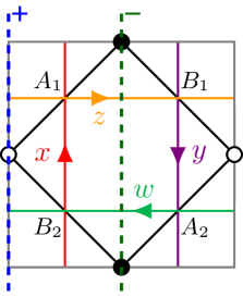
(a) Dimer model.

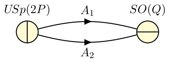
(b) Quiver.

Figure 2: 2(a) Dimer model for the orientifold of the conifold that we are considering. The dashed lines indicate the dimer involution that we are considering (a line orientifold, in the nomenclature of Franco:2007ii ). The solid lines denote the four elementary mesons. We have also named the bifundamentals as in the text. 2(b) The corresponding quiver. We have denoted the bifundamentals with arrows to indicate that they are $\mathcal{N}=1$ chiral multiplets, but they live in real representations so the orientation of the arrow is immaterial.

We are interested in an orientifold action with geometric part acting as

$$\sigma\colon(x,y,z,w)\to(y,x,-z,-w)\,.$$ (9)

In the $z_{4}\neq 0$ patch (and similarly for other patches) the holomorphic three form for the conifold can be written as

$$\Omega=\frac{dz_{1}\wedge dz_{2}\wedge dz_{3}}{z_{4}}$$ (10)

which transforms under (9) as $\Omega\to-\Omega$, as befits an orientifold compatible with the presence of D3-branes. Acting on the singular conifold (7) the involution (9) leaves the origin $x=y=z=w=0$ fixed, while acting on the deformed conifold (8) it leaves two fixed points at $(x,y,z,w)=(\lambda,\lambda,0,0)$ with $\lambda=\pm it$ fixed. The brane tiling and corresponding quiver for the theory of fractional branes on the orientifolded singularity can be determined using the techniques in Franco:2007ii , or more directly via our explicit type IIA construction below.

As is well known, in the absence of the orientifold the deformation of the conifold takes place dynamically due to confinement in the brane system Klebanov:2000hb . The same is true in the presence of the orientifold. Our goal in this section will be to clarify various aspects of the dynamics of this orientifolded configuration. Most importantly for our purposes, we will determine which type of orientifold fixed plane arises after confinement, which we need to know in order to construct explicit embeddings of the nilpotent goldstino.

We will describe the physics of branes in type IIB language momentarily, but we first discuss the physics of the type IIA dual, since it is clearer in many respects.

3.1 Type IIA perspective

Let us start by reviewing well known facts about T-duality on the conifold. The singular conifold $xy=zw$ has a $U(1)$ symmetry

$$(x,y,z,w)\to(e^{i\alpha}x,e^{-i\alpha}y,z,w)\,.$$ (11)

The full symmetry group is $SU(2)\times SU(2)\times U(1)$, as is well known Klebanov:1998hh , but we focus on this subgroup for convenience. We can view (11) as a $\mathbb{C}^{*}$ fibration over $(z,w)$, with the $\mathbb{C}^{*}$ fibre constructed as the hypersurface $xy=zw$ in the $(x,y)$ ambient $\mathbb{C}^{2}$. The $\mathbb{C}^{*}$ fibre becomes singular at $\{z=0\}\cap\{w=0\}$. Fixing a finite radius at infinity, we can T-dualise along this isometry and obtain a IIA dual on $\mathbb{R}^{9}\times S^{1}$, in the presence of NS5 branes located where the $\mathbb{C}^{*}$ fibre (or equivalently the $U(1)$ action (11)) degenerates, i.e. $\{z=0\}\cup\{w=0\}$. The position of the NS5 branes on the fibre directions depends on the value of the $B$-field across the $\mathbb{P}^{1}$ cycle in the resolved description of the conifold. For concreteness, we label the coordinates as $x^{i}$, with $x^{0},\ldots,x^{3}$ the four Minkowski directions, $z=x^{4}+ix^{5}$, $w=x^{8}+ix^{9}$ and $x^{6}\in S^{1}$ the direction on which we T-dualise. We have

$$\begin{array}[]{c|cccccccccc}&0&1&2&3&4&5&6&7&8&9\\ \hline\cr\text{NS5}&-&-&-&-&-&-\\ \text{NS5}^{\prime}&-&-&-&-&&&&&-&-\\ \text{D4}&-&-&-&-&&&-\end{array}$$ (12)

We have also indicated the D4-branes appearing from dualising a D3-brane at the conifold. Fractional D3-branes are D4-branes ending on the NS5 and NS5^′ branes, instead of wrapping fully around the $x^{6}$ direction.

For the purposes of relating the IIA and IIB pictures we write local coordinates $r,s$ for the $\mathbb{C}^{*}$

$$s+ir=\frac{1}{4\pi i}\log\left(\frac{x}{y}\right)\,.$$ (13)

The $U(1)$ isometry acts by shifts on the periodic coordinate $s$, leaving $r$ invariant. (We have introduced an extra factor of $\frac{1}{2}$ so that $s\to s+1$ as we act with a full $U(1)$ rotation.) For finite asymptotic radius of the $\mathbb{C}^{*}$ we have, far enough from the core, a flat $\mathbb{R}\times S^{1}$ geometry parametrised by $(r,s)$. T-duality in this asymptotic region then acts on $s$ only, so we identify $r\cong x^{7}$, and $s$ and $x^{6}$ are coordinates on the T-dual circles.

The complex deformation of the conifold has equation $zw=xy+t^{2}$. For simplicity we will take $t\in\mathbb{R}$. Clearly the isometry (11) is still there, so we can still T-dualise. The picture is similar, but now the two NS5 branes recombine into the smooth 2-cycle $zw=t^{2}$.

The previous discussion has nothing which is not well known. Let us now orientifold the configuration, and see what we obtain. The orientifold action of interest to us is given by $(x,y,z,w)\to(y,x,-z,-w)$ in (9). Exchanging $x$ with $y$, the action on the local coordinates is $(r,s)\to(-r,-s)$. Upon T-duality this maps to $x^{7}\to-x^{7}$. Together with the sign change in $(z,w)$, this gives precisely an O4-plane wrapping $x^{6}$, as expected. Recalling that the orientifold type changes when crossing a NS5 brane, we find a $U\!Sp\times SO$ structure for the gauge algebra on the branes, as in figure 2.

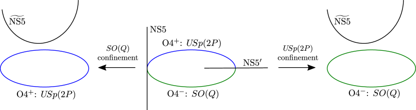
Figure 3: Confinement on the orientifolded conifold from the IIA perspective. The central Hanany-Witten Hanany:1996ie configuration is the classical description. Confinement on the $SO(Q)$ factor (left diagram) corresponds to joining together the NS5 and NS5^′ branes by shrinking to zero size the $SO(Q)$ side (i.e. the side with the O4^- plane), and then recombining the two intersecting NS5 branes into the recombined object $\widetilde{\text{NS5}}$, which does not intersect the remaining O4⁺ plane. Similarly confinement of the $U\!Sp(2P)$ factor (right) leads to a O4^- plane after confinement. In either case, we observe that the remaining O4-plane has sign opposite to the O4-plane on the gauge factor giving rise to confinement.

Now we do the geometric deformation. There are two key facts to observe: the locus $\{zw=t^{2}\}$ wrapped by the NS5 maps to itself under $(z,w)\to(-z,-w)$, but it does so without any fixed points. So the recombined NS5 does not intersect the O4. The two fixed points of the deformed conifold in the $(x,y,z,w)$ coordinates are at $(x,x,0,0)$, with $x=\pm it$. This is at $r=0$, $s=\{0,\frac{1}{2}\}$ in our coordinates above, so we expect that they appear simply from T-dualising the O4 on $x^{6}$ (now with no NS5 branes complicating the discussion). This implies the two fixed points have the same NSNS charge, with an associated projection opposite to that of the gauge factor being confined. Explicitly, this means that if we have a confining $U\!Sp$ group, we end up with two fixed points of type O3^- (with one or both possibly of type $\widetilde{\text{O3}^{-}}$, depending on discrete gauge and RR flux choices). And similarly, if the $SO$ group confines we get two orientifolds of type O3⁺. We have depicted the confining process in the type IIA picture in figure 3.

It may be illuminating to describe more explicitly the fate of the deformation $S^{3}$ after T-duality. The manifold wrapped by the NS5 branes, given by $zw=t^{2}$, has the topology of a smooth $\mathbb{C}^{*}$ when $t\neq 0$. There is a minimal area $S^{1}$ in this $\mathbb{C}^{*}$, which bounds a minimal area disk. T-dualising the $x^{6}$ coordinate over this disk produces in the dual a $S^{1}$ fibration over a disk where the fibre degenerates at the $S^{1}$ boundary of the disk, a well known construction of $S^{3}$.

Let us describe this construction in some detail. We introduce (as we will do in (32) below) the new coordinates

$$z_{i}=(z+w,-i(x+y),x-y,i(w-z))\,.$$ (14)

In these variables the deformed conifold equation can be written as

$$\sum_{i=1}^{4}z_{i}^{2}=4t^{2}\,.$$ (15)

We also have $z_{1}^{2}+z_{4}^{2}=4zw$, so in these variables the NS5 brane in the IIA side is wrapping $z_{1}^{2}+z_{4}^{2}=\frac{1}{4}t^{2}$. We will identify below the $S^{3}$ on the type IIB side as living at $z_{i}\in\mathbb{R}$. This naturally defines a disk $\Re(z_{1})^{2}+\Re(z_{4})^{2}=\rho^{2}$, with $\rho\in[0,\frac{1}{2}t]$, ending on the NS5. T-duality acts as $(z_{1},z_{4})\to(-z_{1},-z_{4})$, so any fixed points must be at the origin of the disk. We expect that in the type IIB picture the fibre over the origin of the disk is the $S^{1}$ parametrised by $s$; we will now verify this. From (15), we have that at the origin of the disk the $S^{1}$ fibre in the $S^{3}$ is given by $\Re(z_{2})^{2}+\Re(z_{3})^{2}=4t^{2}$. The locus $r=0$ corresponds to $(x,y)=(ye^{4\pi is},y)$. We require $xy=-t^{2}$, so $y^{2}e^{4\pi is}=-t^{2}$, or alternatively $y=ite^{-2\pi is}$, $x=ite^{2\pi is}$. Then

$$(\Re(z_{2}),\Re(z_{3}))=(\Im(x+y),\Re(x-y))=(2t\cos(2\pi s),-2t\sin(2\pi s))$$ (16)

precisely according to expectations. So in this notation we see very clearly that the two O3-planes at $s=\{0,\frac{1}{2}\}$ (equivalently, at $\Re(z_{1})=\Re(z_{3})=\Re(z_{4})=0$) arise from T-duality of the O4 wrapping the circle T-dual to the $s$ direction, which implies that they are of the same sign (since in the deformed configuration the NS5 branes do not intersect the O4, so its NSNS charge is the same all along the circle).

3.2 The singular orientifolded conifold in type IIB

We will now reproduce and extend these results directly from the type IIB perspective. There are a number of initially puzzling aspects of the construction when reinterpreted in this context, as we now discuss. We will be using the description of fractional branes as coherent sheaves (see Aspinwall:2002ke for a review which also discusses the conifold explicitly).

Fractional branes and resolved phase

A useful operation from the IIB perspective is the blow-up of the singularity. Geometrically, we can think of the singular conifold as a limit of the blown-up conifold, given by the total space of the $\mathcal{O}(-1)\oplus\mathcal{O}(-1)$ bundle over $\mathbb{P}^{1}$. The conifold singularity appears when the geometric size of the $\mathbb{P}^{1}$ goes to zero. In addition to the geometric volume of the $\mathbb{P}^{1}$ one should also consider the integral of the $B$ field over the $\mathbb{P}^{1}$. We have identified the geometric result of introducing a $B$ field in the T-dual picture in our discussion above: it corresponds to the relative separation of the two NS5 branes along the fibre $S^{1}$. We now would like to identify the effect of geometrically blowing up the $\mathbb{P}^{1}$.

There is basically a unique choice, suggested by analyticity: recall that the homolorphic Kähler coordinate at low energies is $B+iJ$, with $J$ the volume of the $\mathbb{P}^{1}$. Geometrically, the complex coordinate in the T-dualised conifold is given by $x^{6}+ix^{7}$. So, by holomorphicity, we should identify blow-ups of the $\mathbb{P}^{1}$ in the conifold with displacements of the NS5 branes on the $x^{7}$ direction. That this is the right identification can be verified in a number of ways, see for example Giveon:1998sr ; Kutasov:2012rv .

The complexified Kähler moduli space of the conifold can be compactified to a $\mathbb{P}^{1}$. Let us parametrise this $\mathbb{P}^{1}$ of Kähler moduli by a coordinate $\zeta$, with $\zeta=0$ the infinitely blown-up conifold, and $\zeta=\infty$ the infinitely blown-up conifold in the flopped phase. The ordinary $B$ and $J$ Kähler moduli then appear as

$$t\equiv B+iJ=\frac{1}{2\pi i}\log\zeta\,.$$ (17)

The two fractional branes in which a D3 decomposes in the conifold locus can be described in terms of the derived category of coherent sheaves on the resolved conifold $\widetilde{X}$ (choosing a phase) by $\mathcal{O}_{C}(-1)[1]$ and $\mathcal{O}_{C}$, with $C$ the resolution $\mathbb{P}^{1}$. The central charges are fairly easy to compute in this geometry, since they are uncorrected by world-sheet instantons. They are given by the large volume expression

$$Z(\mathcal{O}_{C}(m)[k])=(-1)^{k}(-t+m+1)\,.$$ (18)

We see that the quiver locus, where the central charges of both fractional branes are real, is precisely when $t\in\mathbb{R}$, i.e. $J=0$, as one may have expected. When in addition $B=0$, one finds that some of the fractional branes become massless (mass being given by $|Z|$), so this is a point where light strings can arise. In the type IIA description this corresponds to the locus in moduli space where the $x^{6}$ position of the two NS5 branes coincide.

The type IIA orientifold of interest to us must have a number of surprising features when reinterpreted in the original language of type IIB at singularities. First, notice from the IIA description that the orientifold fixes the NS5 branes to be at $x^{7}=0$, while allowing motions in the $x^{6}$ direction. In IIB language, this can be reinterpreted as the statement that the orientifold projects out the size of the resolution $\mathbb{P}^{1}$, while preserving the integral of the $B$ field as a dynamical field. The same point can be seen already from field theory: the theory with $SO\times U\!Sp$ group does not admit Fayet-Iliopoulos terms (simply because there are no $U(1)$s), so there is no baryonic direction in moduli space. Geometrically, such a baryonic direction would come from blowing up the singularity: this would force misalignment between the fractional branes, since they have opposite BPS phases at large volume. So we also conclude from this perspective that the blow-up mode must be projected out. This is somewhat surprising, and contrary to the usual behavior of ordinary $O3$/$O7$ planes in type IIB.

A more surprising property (but, as we will see, related to the previous point) comes again from the fact that the fractional branes at the conifold admit a description as wrapped D5 and anti-D5 branes. The orientifold that we want must map these fractional branes to themselves, while being compatible with the supersymmetry preserved by a background D3. So at the level of the worldsheet it should act as $\Omega(-1)^{F_{L}}$, while at the same time somehow mapping a fractional D3, which is microscopically a wrapped D5, to itself. Our first goal will be to resolve these tensions.

These issues could be resolved if we take an involution of the resolved $\mathbb{P}^{1}$ that reverses its orientation, such as the $\mathbb{Z}_{2}$ action defining the $\mathbb{P}^{1}\to\mathbb{R}\mathbb{P}^{2}$ map. Under this involution the Fubini-Study metric changes sign. So the combined action of $\Omega$ and the geometric action preserves $B$, but not $J$. And similarly, the D5 wrapping the $\mathbb{P}^{1}$ maps to minus itself, which allows it to survive when combined with the intrinsic minus sign coming from $\Omega(-1)^{F_{L}}$. An ordinary D3 is pointlike, so it also survives. We now show that we do indeed have an orientation reversing involution.

Orientifold geometric involution in the resolved phase

Recall that the geometric action for our orientifold is given by

$$(x,y,z,w)\to(y,x,-z,-w)\,.$$ (19)

It will be useful to rewrite this action in terms of GLSM fields. The conifold is described by a GLSM with fields $(x_{1},x_{2},y_{1},y_{2})$ with charges $(1,1,-1,-1)$ under a $U(1)$ gauge group. We take the FI term to be according to

$$V_{D}=\left(|x_{1}|^{2}+|x_{2}|^{2}-|y_{1}|^{2}-|y_{2}|^{2}-\xi\right)^{2}$$ (20)

and the map to the gauge invariant coordinates to be

$$(x,y,z,w)=(x_{1}y_{2},x_{2}y_{1},x_{1}y_{1},x_{2}y_{2})\,.$$ (21)

In these coordinates, the action (19) is described by

$$\sigma\colon(x_{1},x_{2},y_{1},y_{2})\to(-y_{1},y_{2},x_{1},-x_{2})\,.$$ (22)

There are various things to note in this expression. First, it is a well defined $\mathbb{Z}_{2}$ action when we take the $U(1)$ gauge symmetry into account: orbits are mapped to orbits. (Even if $\sigma^{2}=-1$.)

The D-term changes sign, though: if we have a point satisfying the D-term with $\xi>0$, it will get mapped to a point satisfying the D-term with $\xi<0$. In other words, the $\mathbb{Z}_{2}$ action defines an involution of the conifold only for the singular conifold, with $\xi=0$. If $\xi\neq 0$, so we are in some resolved phase, the $\mathbb{Z}_{2}$ action maps to the flopped phase: $\xi\to-\xi$. Since $\xi$ can be interpreted as the volume of the resolved $\mathbb{P}^{1}$, this action achieves precisely what we expected from the general arguments above: $J=0$ but $B$ is arbitrary, since the volume form in $\mathbb{P}^{1}$ geometrically changes sign. In the algebraic language, the statement is that the $\mathbb{Z}_{2}$ acts on the Stanley-Reisner ideal: it exchanges the Stanley-Reisner ideal $\left\langle x_{1}x_{2}\right\rangle$ of a resolved phase ($\xi>0$) with the Stanley-Reisner ideal $\left\langle y_{1}y_{2}\right\rangle$ of the flopped phase ($\xi<0$).

For later purposes it will also be useful to describe in more detail the action of the orientifold on the geometry, which will also give an explicit proof of the inversion of the volume element of the resolution $\mathbb{P}^{1}$. In particular, we will now describe how the involution (22) acts on the conifold seen as the real cone over $S^{2}\times S^{3}$. We start by reviewing how to go from the GLSM description in terms of the $x_{i},y_{i}$ variables to the description in terms of a real cone over $S^{2}\times S^{3}$. (The following discussion of the unorientifolded geometry summarises Evslin:2007ux ; Evslin:2008ve , although we deviate slightly from the presentation there in order to highlight some aspects of the construction that will become useful to us later.) We will do the calculation for the singular conifold $\xi=0$. The horizon $S^{2}\times S^{3}$ at a radial distance $r$ is obtained by imposing

$$|x_{1}|^{2}+|x_{2}|^{2}=|y_{1}|^{2}+|y_{2}|^{2}=r\,.$$ (23)

We will work at $r=1$ for simplicity. Start by introducing the matrices

$$\begin{split}U&=\begin{pmatrix}x_{1}&-\overline{x_{2}}\\ x_{2}&\overline{x_{1}}\end{pmatrix}\,,\\ V&=\begin{pmatrix}\overline{y_{1}}&-y_{2}\\ \overline{y_{2}}&y_{1}\end{pmatrix}\,.\end{split}$$ (24)

It is a simple calculation to show that on the horizon these two matrices belong to $SU(2)$. Under the $U(1)$ action of the GLSM they transform as $U\to Ue^{i\alpha\sigma_{3}}$, $V\to Ve^{i\alpha\sigma_{3}}$, with $\sigma_{3}=\left(\begin{smallmatrix}1&0\\ 0&-1\end{smallmatrix}\right)$ the third Pauli matrix. Introduce now the gauge invariants

$$\begin{split}X&=UV^{\dagger}\,,\\ Y&=-iU\sigma_{3}V^{\dagger}\,.\end{split}$$ (25)

These matrices also clearly belong to $SU(2)$. Following Evslin:2007ux , we also introduce

$$Q=X^{\dagger}Y=-iV\sigma_{3}V^{\dagger}\,,$$ (26)

which is nothing but the Hopf projection of $V\in SU(2)=S^{3}\to S^{2}$. It is clear from the second expression that in addition to being an element of $SU(2)$, $Q$ is traceless, anti-hermitian, and squares to $-1$. One can also easily see that there is a bijection between the pair $(X,Q)$ and the usual set of coordinates for the conifold

$$W=\begin{pmatrix}x_{1}y_{1}&x_{1}y_{2}\\ x_{2}y_{1}&x_{2}y_{2}\end{pmatrix}=\frac{1}{2}(X+iY)=\frac{1}{2}X({\bf 1}+iQ)\,.$$ (27)

That the bijection exists is manifest if we construct $X$, $Y$ in terms of $W$ as follows

$$\begin{split}X&=\operatorname{Tr}W^{\dagger}+W-W^{\dagger}\\ Y&=i\operatorname{Tr}W^{\dagger}-i(W-W^{\dagger})\,.\end{split}$$ (28)

Now, $X$ and $Q$ are independent, so they parametrise a product space. $X$ is a generic $SU(2)$ matrix, so it parametrises a $S^{3}$, while the condition that $Q$ is a traceless $SU(2)$ matrix implies that it parametrises an $S^{2}$. We thus have a good set of coordinates for $S^{2}\times S^{3}$, and we showed explicitly the diffeomorphism to the conifold base in the usual coordinates. It will be convenient to be more explicit about the coordinates of the spheres. For a generic $SU(2)$ matrix $S$ one has the Pauli decomposition

$$S=S_{0}+i\sum_{i=1}^{3}S_{i}\sigma_{i}$$ (29)

with $\sigma_{i}$ the Pauli matrices, $S_{0}=\frac{1}{2}\operatorname{Tr}S$, $S_{i}=-\frac{i}{2}\operatorname{Tr}(S\sigma_{i})$. $\det S=1$ implies $\sum_{\mu=0}^{3}S_{\mu}^{2}=1$, which is the usual equation of $S^{3}\subset\mathbb{R}^{4}$. Imposing tracelessness of $S$, as for $Q$, sets $S_{0}=0$, and thus gives a $S^{2}\subset S^{3}$, as we claimed above. In what follows we denote by $U_{\mu},V_{\mu},X_{\mu},Y_{\mu},Q_{\mu}$ the components of the $SU(2)$ matrices $U,V,X,Y,Q$ in this basis.

With this description of the $S^{2}\times S^{3}$ horizon of the conifold in hand we can come back to the orientifold action (22). In terms of the projective coordinates

$$\begin{split}X_{\mu}&=\biggl{(}\frac{1}{2}\,x_{1}y_{1}+\frac{1}{2}\,x_{2}y_{2}+\frac{1}{2}\,\overline{x_{1}}\overline{y_{1}}+\frac{1}{2}\,\overline{x_{2}}\overline{y_{2}}\,,\\ &\phantom{=\biggl{(}}-\frac{1}{2}i\,x_{2}y_{1}-\frac{1}{2}i\,x_{1}y_{2}+\frac{1}{2}i\,\overline{x_{2}}\overline{y_{1}}+\frac{1}{2}i\,\overline{x_{1}}\overline{y_{2}}\,,\\ &\phantom{=\biggl{(}}-\frac{1}{2}\,x_{2}y_{1}+\frac{1}{2}\,x_{1}y_{2}-\frac{1}{2}\,\overline{x_{2}}\overline{y_{1}}+\frac{1}{2}\,\overline{x_{1}}\overline{y_{2}}\,,\\ &\phantom{=\biggl{(}}-\frac{1}{2}i\,x_{1}y_{1}+\frac{1}{2}i\,x_{2}y_{2}+\frac{1}{2}i\,\overline{x_{1}}\overline{y_{1}}-\frac{1}{2}i\,\overline{x_{2}}\overline{y_{2}}\biggr{)}\,.\end{split}$$ (30)

We can rewrite this equation in terms of the GLSM invariant coordinates $x,y,z,w$ as

$$X_{\mu}=(\Re(z+w),\Im(x+y),\Re(x-y),\Im(z-w))\,.$$ (31)

This suggests introducing the new variables

$$z_{i}=(z+w,-i(x+y),x-y,i(w-z))\,,$$ (32)

so that

$$X_{\mu}=(\Re(z_{1}),\Re(z_{2}),\Re(z_{3}),\Re(z_{4}))\,.$$ (33)

In terms of these variables the conifold equation $xy=zw$ becomes

$$\sum_{i=1}^{4}z_{i}^{2}=0\,,$$ (34)

and the deformed conifold equation $zw=xy+t^{2}$ becomes

$$\sum_{i=1}^{4}z_{i}^{2}=4t^{2}\,.$$ (35)

The involution (19) acts on these variables as

$$z_{i}\to(-z_{1},z_{2},-z_{3},-z_{4})\,.$$ (36)

From here, or directly doing a bit of algebra on (30), one finds that the action (22) on the $S^{3}$ coordinates $X$ is given by

$$X_{\mu}\to(-X_{0},X_{1},-X_{2},-X_{3})$$ (37)

which has fixed points (forgetting about the $S^{2}$ momentarily) at $X_{0}=X_{2}=X_{3}=0$, i.e. two points in the $S^{3}$. This agrees with the fixed point structure we found from our type IIA picture in §3.1.

Let us study the structure of the $S^{2}$ component at one of these fixed points in the $S^{3}$. Going to the patch $x_{1}\neq 0$ we can gauge fix $x_{1}$ to be real and positive. A solution to $X_{0}=X_{2}=X_{3}=0$ can then be found at $(x_{1},x_{2},y_{1},y_{2})=(1,0,0,i)$, which maps to $X_{\mu}=(0,1,0,0)$. As a small consistency check, notice that the action of (22) on this point gives $(x_{1},x_{2},y_{1},y_{2})=(0,i,1,0)$, which again maps to $X_{\mu}=(0,1,0,0)$, but as expected acts freely on the total space $S^{3}\times S^{2}$. To reconstruct the whole $\mathbb{P}^{1}$ we start with the point $(x_{1},x_{2},y_{1},y_{2})=(1,0,0,i)$, giving

$$U_{0}=\begin{pmatrix}1&0\\ 0&1\end{pmatrix}=\sigma_{0}\qquad;\qquad V_{0}=\begin{pmatrix}0&-i\\ -i&0\end{pmatrix}=-i\sigma_{1}\,.$$ (38)

Tracing through the definitions, this gives $X=i\sigma_{1}$, $Y=i\sigma_{2}$ and $Q=i\sigma_{3}$. Any other point in the $\mathbb{P}^{1}$ above $(U_{0},V_{0})$ can be written as $(U,V)=(U_{0}g,V_{0}g)$ for some $g\in SU(2)$. This leaves $X=U_{0}V_{0}^{\dagger}$ invariant, but introduces a dependence of $Q=-i\sigma_{1}g\sigma_{3}g^{-1}\sigma_{1}$ on $g$.

In terms of $U,V$ the action (22) acts as

$$U\to-\sigma_{1}V\sigma_{1}\qquad;\qquad V\to\sigma_{1}U\sigma_{1}$$ (39)

so it sends

$$Q=-iV\sigma_{3}V^{\dagger}\to-i\sigma_{1}U\sigma_{1}\sigma_{3}\sigma_{1}U^{\dagger}\sigma_{1}=i\sigma_{1}U\sigma_{3}U^{\dagger}\sigma_{1}$$ (40)

which for the $\mathbb{P}^{1}$ we are studying reduces to

$$Q_{g}=-i\sigma_{1}g\sigma_{3}g^{-1}\sigma_{1}\to i\sigma_{1}g\sigma_{3}g^{-1}\sigma_{1}=-Q_{g}\,.$$ (41)

So we learn that the action of the involution on the $\mathbb{P}^{1}$ above $(U_{0},V_{0})$ is the orientation-reversing $\mathbb{P}^{1}\to\mathbb{R}\mathbb{P}^{2}$ map, as we guessed above based on the IIA dual and microscopic considerations. There is also a second fixed point at $X_{\mu}=(0,-1,0,0)$, for which a very similar discussion applies.

3.3 The orientifolded cascade

The discussion in the previous section was about the singular conifold. In analogy with the behavior in absence of the orientifold Klebanov:2000hb , for nontrivial fractional brane configurations the orientifolded conifold is deformed dynamically. In this section, we want to study this effect from the field theory point of view. In particular, by this method we will verify the prediction for the orientifold charges given in §3.1. Useful references for this section are Dymarsky:2005xt ; Krishnan:2008gx .

Classical dynamics

The dimer model and the quiver describing the low energy dynamics for D3-branes on the orientifold of the conifold we are studying were given in figure 2. The superpotential for the resulting theory is somewhat subtle, but its form is important for the considerations below, so let us derive it in some detail. We parametrise the fields of the $SU(N)\times SU(M)$ theory before taking the orientifold as $A_{i},B_{i}$, with $A_{i}\in(\leavevmode\hbox{$\vbox{\hbox{\vtop{ \offinterlineskip\openup-0.39993pt\halign{&\opttoksa@YT={\font@YT}\getcolor@YT{\save@YT{\opttoksb@YT}}\nil@YT\getcolor@YT{\startbox@@YT\the\opttoksa@YT\the\opttoksb@YT}#\endbox@YT\cr\lower 0.39993pt\vbox{\kern 0.19997pt\hbox{\kern 0.39993pt\vbox to5.39993pt{\vss\hbox to5.0pt{\hss$$\hss}\vss}\kern-5.39993pt\vrule height=5.39993pt,width=0.39993pt\kern 5.0pt\vrule height=5.39993pt,width=0.39993pt}\kern-0.19997pt\kern-5.39993pt\hrule width=5.79987pt,height=0.39993pt\kern 5.0pt\hrule width=5.79987pt,height=0.39993pt}\cr}}\kern 6.19986pt}}$}_{M},\overline{\leavevmode\hbox{$\vbox{\hbox{\vtop{ \offinterlineskip\openup-0.39993pt\halign{&\opttoksa@YT={\font@YT}\getcolor@YT{\save@YT{\opttoksb@YT}}\nil@YT\getcolor@YT{\startbox@@YT\the\opttoksa@YT\the\opttoksb@YT}#\endbox@YT\cr\lower 0.39993pt\vbox{\kern 0.19997pt\hbox{\kern 0.39993pt\vbox to5.39993pt{\vss\hbox to5.0pt{\hss$$\hss}\vss}\kern-5.39993pt\vrule height=5.39993pt,width=0.39993pt\kern 5.0pt\vrule height=5.39993pt,width=0.39993pt}\kern-0.19997pt\kern-5.39993pt\hrule width=5.79987pt,height=0.39993pt\kern 5.0pt\hrule width=5.79987pt,height=0.39993pt}\cr}}\hbox{\vtop{ \offinterlineskip\openup-0.39993pt\halign{&\opttoksa@YT={\font@YT}\getcolor@YT{\save@YT{\opttoksb@YT}}\nil@YT\getcolor@YT{\startbox@@YT\the\opttoksa@YT\the\opttoksb@YT}#\endbox@YT\cr\lower 0.39993pt\vbox{\kern 0.19997pt\hbox{\kern 0.39993pt\vbox to5.39993pt{\vss\hbox to5.0pt{\hss$$\hss}\vss}\kern-5.39993pt\vrule height=5.39993pt,width=0.39993pt\kern 5.0pt\vrule height=5.39993pt,width=0.39993pt}\kern-0.19997pt\kern-5.39993pt\hrule width=5.79987pt,height=0.39993pt\kern 5.0pt\hrule width=5.79987pt,height=0.39993pt}\cr}}\kern 6.19986pt}\kern 6.19986pt}}$}}_{N})$ and $B_{i}\in(\overline{}\leavevmode\hbox{$\vbox{\hbox{\vtop{ \offinterlineskip\openup-0.39993pt\halign{&\opttoksa@YT={\font@YT}\getcolor@YT{\save@YT{\opttoksb@YT}}\nil@YT\getcolor@YT{\startbox@@YT\the\opttoksa@YT\the\opttoksb@YT}#\endbox@YT\cr\lower 0.39993pt\vbox{\kern 0.19997pt\hbox{\kern 0.39993pt\vbox to5.39993pt{\vss\hbox to5.0pt{\hss$$\hss}\vss}\kern-5.39993pt\vrule height=5.39993pt,width=0.39993pt\kern 5.0pt\vrule height=5.39993pt,width=0.39993pt}\kern-0.19997pt\kern-5.39993pt\hrule width=5.79987pt,height=0.39993pt\kern 5.0pt\hrule width=5.79987pt,height=0.39993pt}\cr}}\kern 6.19986pt}}$}_{M},\leavevmode\hbox{$\vbox{\hbox{\vtop{ \offinterlineskip\openup-0.39993pt\halign{&\opttoksa@YT={\font@YT}\getcolor@YT{\save@YT{\opttoksb@YT}}\nil@YT\getcolor@YT{\startbox@@YT\the\opttoksa@YT\the\opttoksb@YT}#\endbox@YT\cr\lower 0.39993pt\vbox{\kern 0.19997pt\hbox{\kern 0.39993pt\vbox to5.39993pt{\vss\hbox to5.0pt{\hss$$\hss}\vss}\kern-5.39993pt\vrule height=5.39993pt,width=0.39993pt\kern 5.0pt\vrule height=5.39993pt,width=0.39993pt}\kern-0.19997pt\kern-5.39993pt\hrule width=5.79987pt,height=0.39993pt\kern 5.0pt\hrule width=5.79987pt,height=0.39993pt}\cr}}\hbox{\vtop{ \offinterlineskip\openup-0.39993pt\halign{&\opttoksa@YT={\font@YT}\getcolor@YT{\save@YT{\opttoksb@YT}}\nil@YT\getcolor@YT{\startbox@@YT\the\opttoksa@YT\the\opttoksb@YT}#\endbox@YT\cr\lower 0.39993pt\vbox{\kern 0.19997pt\hbox{\kern 0.39993pt\vbox to5.39993pt{\vss\hbox to5.0pt{\hss$$\hss}\vss}\kern-5.39993pt\vrule height=5.39993pt,width=0.39993pt\kern 5.0pt\vrule height=5.39993pt,width=0.39993pt}\kern-0.19997pt\kern-5.39993pt\hrule width=5.79987pt,height=0.39993pt\kern 5.0pt\hrule width=5.79987pt,height=0.39993pt}\cr}}\kern 6.19986pt}\kern 6.19986pt}}$}_{N})$. The superpotential for this theory is well known Klebanov:1998hh :

$$W=\frac{1}{2}\varepsilon_{ij}\varepsilon_{lm}\operatorname{Tr}\left(A_{i}B_{l}A_{j}B_{m}\right)=\operatorname{Tr}\left(A_{1}B_{1}A_{2}B_{2}-B_{2}A_{2}B_{1}A_{1}\right)\,.$$ (42)

There is a $SO(4)=SU(2)_{1}\times SU(2)_{2}$ global symmetry of the singular conifold. In terms of the GLSM it manifests itself as $(x_{i},y_{i})\to(g_{1}\bm{x},g_{2}\bm{y})$, with $g_{i}\in SU(2)_{i}$ in the fundamental representation, and $\bm{x}=(x_{1},x_{2})$, $\bm{y}=(y_{1},y_{2})$. For the case $N=M=1$ of a single brane probing the conifold we can identify $\left\langle A_{i}\right\rangle=x_{i}$, $\left\langle B_{i}\right\rangle=y_{i}$. The involution (22) can be written in these variables as

$$\sigma\colon(\bm{x},\bm{y})\to(-\sigma_{3}\bm{y},\sigma_{3}\bm{x})\,.$$ (43)

We want to determine the subgroup $G\subset SU(2)_{1}\times SU(2)_{2}$ compatible with $\sigma$. That is, for every $g\in G$, $\sigma g=g\sigma$, modulo the $U(1)$ GLSM action $(\bm{x},\bm{y})\to(e^{i\alpha}\bm{x},e^{-i\alpha}\bm{y})$. Equivalently, in block matrix form

$$\begin{pmatrix}g_{1}&0\\ 0&g_{2}\end{pmatrix}=-\begin{pmatrix}0&-\sigma_{3}\\ \sigma_{3}&0\end{pmatrix}\begin{pmatrix}g_{1}&0\\ 0&g_{2}\end{pmatrix}\begin{pmatrix}0&-\sigma_{3}\\ \sigma_{3}&0\end{pmatrix}=\begin{pmatrix}\sigma_{3}g_{2}\sigma_{3}&0\\ 0&\sigma_{3}g_{1}\sigma_{3}\end{pmatrix}$$ (44)

which can be satisfied by $g_{1}=\sigma_{3}g_{2}\sigma_{3}$. Parametrising $g_{1}=a_{0}+i\sum_{k=1}^{3}a_{k}\sigma_{k}$, $g_{2}=b_{0}+i\sum_{k=1}^{3}b_{k}\sigma_{k}$ (with $\sum a_{\mu}^{2}=\sum b_{\mu}^{2}=1$), this requires $(a_{0},a_{1},a_{2},a_{3})=(b_{0},-b_{1},-b_{2},b_{3})$. So we learn that $SU(2)_{d}\subset G$ is conserved by the orientifold action.

Let us come back to the field theory arising after orientifolding, described by the quiver in figure 2(b). From the action of the involution on the dimer model in figure 2(a) we immediately read that the invariant fields under the involution satisfy

$$\begin{split}B_{1}&=s_{1}\gamma_{U\!Sp}A_{1}^{t}\gamma_{SO}\,,\\ B_{2}&=s_{2}\gamma_{U\!Sp}A_{2}^{t}\gamma_{SO}\,.\end{split}$$ (45)

We take the following block-diagonal representation for the Chan-Paton matrices

$$\gamma_{SO}=\bm{1}\qquad;\qquad\gamma_{U\!Sp}=\begin{pmatrix}\sigma_{2}\\ &\sigma_{2}\\ &&\ddots\\ &&&\sigma_{2}\end{pmatrix}$$ (46)

with $\sigma_{2}=\left(\begin{smallmatrix}0&-i\\ i&0\end{smallmatrix}\right)$ for the action of the orientifold on the gauge factors. The transpose in (45) is, as usual, coming from the reflection of the worldsheet. We have additionally included a possible sign $s_{i}=\pm 1$ for completeness. We can nevertheless now use our observation of the presence of the $SU(2)_{d}$ symmetry after orientifolding to impose $s_{1}=s_{2}$, and then redefine these signs away. We will set $s_{i}=+1$ in what follows.

We thus find that the superpotential after orientifolding is

$$\begin{split}W&=\frac{1}{4}\varepsilon_{ij}\varepsilon_{lm}\operatorname{Tr}\left(A_{i}\gamma_{U\!Sp}A_{l}^{t}\gamma_{SO}A_{j}\gamma_{U\!Sp}A_{m}^{t}\gamma_{SO}\right)\,.\end{split}$$ (47)

As one may have guessed, this is the projection of the original superpotential to the invariant fields, and it preserves the $SU(2)$ symmetry we have identified geometrically above.

Let us try to gain some intuition for this theory, before we start analysing the cascade. A simple thing to try is to construct the classical moduli space of a single mobile brane probing the geometry. (The following analysis was also done in Imai:2001cq , but the details of the argument will be slightly different since our convention (46) for the Chan-Paton matrices is different, so we include it here since it may be illuminating for later discussion.)

When the brane is at the singularity, the gauge algebra is $\mathfrak{so}(2)\oplus\mathfrak{usp}(2)$. (The gauge group has in addition a gauged $\mathbb{Z}_{2}$ external automorphism, and is more precisely $O(2)\times U\!Sp(2)$.) In this case we can treat the $A_{i}$ fields as $2\times 2$ matrices, transforming under $(g,h)\in O(2)\times U\!Sp(2)$ as $A_{k}\to gA_{k}h$. The non-abelian D-terms for $\mathfrak{so}(2)$ are

$$\sum_{k=1}^{2}\operatorname{Tr}(A_{k}^{\dagger}\sigma_{2}A_{k})=0\>,$$ (48)

while the non-abelian D-terms for $\mathfrak{usp}(2)$ are

$$\sum_{k=1}^{2}\operatorname{Tr}(A_{k}\sigma_{i}A_{k}^{\dagger})=0$$ (49)

for any Pauli matrix $\sigma_{i}$.

A generic solution of the F-term coming from (47), together with the D-terms (48) and (49) can be written as

$$A_{1}=\begin{pmatrix}\mathsf{x}_{1}&\mathsf{y}_{1}\\ i\mathsf{x}_{1}&-i\mathsf{y}_{1}\end{pmatrix}\,\qquad\qquad A_{2}=\begin{pmatrix}\mathsf{x}_{2}&\mathsf{y}_{2}\\ i\mathsf{x}_{2}&-i\mathsf{y}_{2}\end{pmatrix}\,,$$ (50)

subject to the condition

$$|\mathsf{x}_{1}|^{2}+|\mathsf{x}_{2}|^{2}-|\mathsf{y}_{1}|^{2}-|\mathsf{y}_{2}|^{2}=0\,.$$ (51)

We still have a remnant of the $O(2)\times U\!Sp(2)$ symmetry acting on $A_{i}$, while keeping the form (50). These are $U\!Sp(2)$ transformations acting as

$$A_{1}\to A_{1}\begin{pmatrix}e^{i\alpha}&0\\ 0&e^{-i\alpha}\end{pmatrix}$$ (52)

which in terms of the $\mathsf{x}_{i},\mathsf{y}_{i}$ components is $(\mathsf{x}_{1},\mathsf{x}_{2},\mathsf{y}_{1},\mathsf{y}_{2})\to(e^{i\alpha}\mathsf{x}_{1},e^{i\alpha}\mathsf{x}_{2},e^{-i\alpha}\mathsf{y}_{1},e^{-i\alpha}\mathsf{y}_{2})$. This, together with the D-term (51), reproduces the standard GLSM construction for the singular conifold. In addition, we have the external $\mathbb{Z}_{2}$ automorphism, which acts as $A_{i}\to\sigma_{3}A_{i}$. Combining this action with an appropriate $U\!Sp(2)$ transformation we obtain an extra $\mathbb{Z}_{2}$ action leaving the form of the solution (50) invariant

$$A_{i}\to\sigma_{3}A_{i}(i\sigma_{2})=\begin{pmatrix}-\mathsf{y}_{i}&\mathsf{x}_{i}\\ -i\mathsf{y}_{i}&-i\mathsf{x}_{i}\end{pmatrix}$$ (53)

or directly in terms of the GLSM coordinates $(\mathsf{x}_{i},\mathsf{y}_{i})\to(-\mathsf{y}_{i},\mathsf{x}_{i})$, which perfectly reproduces (22) (up to a harmless sign redefinition).

Quantum dynamics

Now that we have an understanding of the single probe brane case in the classical setting, let us move on to the calculation of interest, namely the determination of the properties of the mesonic branch of the deformed orientifolded conifold, when we have more than one mobile brane probing the dynamics. (We take more than one brane in order to be able to more clearly study $O$ and $U\!Sp$ enhancements at the conifold loci.) The case without the orientifold has been extensively studied, some useful references are Klebanov:2000hb ; Dymarsky:2005xt ; Krishnan:2008gx . The orientifolded case has been studied (in part, we will need to extend the analysis) in Imai:2001cq . A first easy observation is that the seem to be various basic channels for confinement in the $O(Q)\times U\!Sp(2P)$ theory. If $Q\gg P$ the $O(Q)$ node will confine first, and we will end up with a theory of $U\!Sp(2P)$ adjoint mesons. Similarly, if $P\gg Q$ confinement in the $U\!Sp(2P)$ node will occur first, so we will have a theory of $O(Q)$ adjoint mesons.

We want to understand the nature of the O3-planes after confinement in each of these cases. From the IIA perspective we expect that when $U\!Sp(2P)$ confinement dominates we end up with O3^- planes. In the case where $Q\in 2\mathbb{Z}$ we expect the two O3^- planes to be of the same type (either both O3^- or both $\widetilde{\text{O3}}^{-}$), while in the $Q\in 2\mathbb{Z}+1$ we expect one O3^- and one $\widetilde{\text{O3}}^{-}$. In the case where the $O(Q)$ node confines first we expect the two O3-planes to be O3⁺. In this case we cannot say whether they are O3⁺ or $\widetilde{\text{O3}}^{+}$ with the techniques in this section, since they lead to identical perturbative physics, but this distinction is not interesting for our model building purposes in any case.

We will focus on $U\!Sp(2P)$ confinement driving the dynamics. In order to have a weakly coupled geometry after confinement we require $P\gg 1$. In this case we expect to end up with two O3^- planes of the same or different type, depending on the parity of $Q$. We choose to analyze $Q\in 2\mathbb{Z}$, since it makes the analysis a little bit simpler, and is seems to be the most convenient one for model building purposes: the D3 charge of the orientifold system is integral, as opposed to half-integral. The rest of the cases can be analysed very similarly, confirming the IIA predictions just mentioned, so we omit their explicit discussion.

The confined description is in terms of gauge invariant mesons

$$\mathcal{M}_{ij}=A_{i}\gamma_{U\!Sp}A_{j}^{t}\,.$$ (54)

In order to understand the dynamics of the probe stack, consider again the classical moduli space of a stack of $k$ mobile D3-branes. We can construct it by choosing block-diagonal and equal vevs for the $2k\times(2P+2k)$ matrix $A_{i}$

$$A_{i}=\begin{pmatrix}\bm{\mathsf{x}}_{i}&&&&\bm{0}_{k,2P}\\ &\bm{\mathsf{x}}_{i}&&&\bm{0}_{k,2P}\\ &&\ddots&&\vdots\\ &&&\bm{\mathsf{x}}_{i}&\bm{0}_{k,2P}\end{pmatrix}$$ (55)

with $\bm{0}_{r,s}$ is the $r\times s$ zero matrix, and

$$\bm{\mathsf{x}}_{i}=\begin{pmatrix}\mathsf{x}_{i}&\mathsf{y}_{i}\\ i\mathsf{x}_{i}&-i\mathsf{y}_{i}\end{pmatrix}$$ (56)

as in (50). The classical $U\!Sp$ mesons, transforming in the adjoint of $O(2k)$, are given by

$$\mathcal{M}_{ij}=\underbrace{\begin{pmatrix}\bm{\mathsf{x}}_{i}\sigma_{2}\bm{\mathsf{x}}_{j}^{t}\\ &\bm{\mathsf{x}}_{i}\sigma_{2}\bm{\mathsf{x}}_{j}^{t}\\ &&\ddots\\ &&&\bm{\mathsf{x}}_{i}\sigma_{2}\bm{\mathsf{x}}_{j}^{t}\end{pmatrix}}_{k\text{ blocks}}\,.$$ (57)

In the confined description the mesons become elementary fields. The classical picture suggests parametrising the moduli space of mesons in the following way. Introduce the basic elementary meson $\mathsf{z}_{ij}$, which in the classical limit can be written as

$$\mathsf{z}=\begin{pmatrix}\mathsf{x}_{1}\mathsf{y}_{1}&\mathsf{x}_{1}\mathsf{y}_{2}\\ \mathsf{x}_{2}\mathsf{y}_{1}&\mathsf{x}_{2}\mathsf{y}_{2}\end{pmatrix}\,.$$ (58)

We parametrise the possible space of vacua by rewriting the classical expressions for the mesons in (57) by their expression in terms of the fundamental mesons $\mathsf{z}_{ij}$:

$$\mathcal{M}_{ij}=\begin{pmatrix}\bm{\mathsf{m}}_{ij}\\ &\ddots\\ &&\bm{\mathsf{m}}_{ij}\end{pmatrix}$$ (59)

with

$$\begin{split}\bm{\mathsf{m}}_{11}=\begin{pmatrix}0&-2\mathsf{z}_{11}\\ 2\mathsf{z}_{11}&0\end{pmatrix}\quad&;\quad\bm{\mathsf{m}}_{12}=\begin{pmatrix}i(\mathsf{z}_{21}-\mathsf{z}_{12})&-(\mathsf{z}_{12}+\mathsf{z}_{21})\\ \mathsf{z}_{12}+\mathsf{z}_{21}&i(\mathsf{z}_{21}-\mathsf{z}_{12})\end{pmatrix}\\ \bm{\mathsf{m}}_{21}=\begin{pmatrix}i(\mathsf{z}_{12}-\mathsf{z}_{21})&-(\mathsf{z}_{12}+\mathsf{z}_{21})\\ \mathsf{z}_{12}+\mathsf{z}_{21}&i(\mathsf{z}_{12}-\mathsf{z}_{21})\end{pmatrix}\quad&;\quad\bm{\mathsf{m}}_{22}=\begin{pmatrix}0&-2\mathsf{z}_{22}\\ 2\mathsf{z}_{22}&0\end{pmatrix}\end{split}$$ (60)

One can easily see that these vevs satisfy the non-abelian D-term conditions for $O(2k)$. The F-terms are satisfied as follows. In the confined mesonic variables the classical superpotential (47) becomes

$$W=\frac{1}{4}\varepsilon_{ij}\varepsilon_{lm}\operatorname{Tr}\left(\mathcal{M}_{il}\gamma_{SO}\mathcal{M}_{jm}\gamma_{SO}\right)\,.$$ (61)

It is well know that this superpotential gets modified non-perturbatively to Terning:2003th

$$W=\frac{1}{4}\varepsilon_{ij}\varepsilon_{lm}\operatorname{Tr}\left(\mathcal{M}_{il}\gamma_{SO}\mathcal{M}_{jm}\gamma_{SO}\right)+\left(\frac{\Lambda^{\frac{b}{2}}}{\operatorname{Pf}([\mathcal{M}])}\right)^{\frac{1}{P-k+1}}$$ (62)

with $\Lambda$ the dynamical scale of the $U\!Sp$ node, $b=2(3P+k+3)$ the one-loop $\beta$ function coefficient of the $U\!Sp$ theory, and

$$[\mathcal{M}]=\begin{pmatrix}\mathcal{M}_{11}&\mathcal{M}_{12}\\ \mathcal{M}_{21}&\mathcal{M}_{22}\end{pmatrix}\,.$$ (63)

The F-term equations then imply for the ansatz (59) that

$$\det(\mathsf{z})=\Lambda^{\frac{b}{2(P+1)}}$$ (64)

ignoring some irrelevant numerical constants. This is precisely the equation for the deformed conifold, with the small subtlety of the presence of a branch structure (due to the $2(P+1)$-th root), associated with the flux appearing after confinement Klebanov:2000hb .

In order to determine the nature of the orientifolds we need to determine the subgroup of $O(2k)$ leaving invariant all the meson vevs (57) for all points in the moduli space. It is not hard to see that at generic points in moduli space the preserved gauge symmetry is $U(k)$. We interpret this as the $U(k)$ theory on the D3 probe stack away from any enhancement points.

In the current field theory conventions, the orientifold involution (encoded in the $\mathbb{Z}_{2}$ automorphism part of the $O(2k)$ gauge group) acts on the moduli space as

$$(z_{11},z_{12},z_{21},z_{22})\to(-z_{11},-z_{21},-z_{12},-z_{22})$$ (65)

so there are fixed points of the involution at $z_{11}=z_{22}=0$, $z_{12}=-z_{21}$. Notice from (64) that there are exactly two such points in the moduli space for each branch of moduli space, coming from $\mathsf{z}_{12}^{2}=\Lambda^{\frac{b}{2(P+1)}}$. At these two points in moduli space we have $\mathcal{M}_{11}=\mathcal{M}_{22}=0$, and $\mathcal{M}_{12}=-\mathcal{M}_{21}\propto\bm{1}$, so the $O(2k)$ gauge group is unbroken. The natural interpretation of these points in moduli space is as the locations where the probe stack of branes comes on top of the two orientifold planes that we expect. Since both enhancements are to $O(2k)$, this shows that both orientifold planes are O3^- planes.

3.4 Orientifold type changing transitions

There is one small loose end in this whole discussion. Assume that we do not put any (fractional or regular) branes on the conifold. It seems like we have a choice in whether we deform into the configuration with two O3^- or two O3⁺ planes, and furthermore, these two configurations seem to be smoothly connected by a local operation on the conifold. On the other hand, these two configurations have opposite RR charge, differing in the charge of a mobile D3. This is measurable asymptotically, so we have a puzzle.

A careful formulation of the puzzle leads almost immediately to the solution. Notice that, since the O4^- and O4⁺ planes have opposite RR charge, in the absence of fractional branes the type IIA configuration does not have the same tension on both sides of the NS5 branes, and the O4⁺ side will tend to confine. This may perhaps sounds surprising, but it is a manifestation of the fact that isolated $U\!Sp(0)$ nodes in string theory behave as if there was gaugino condensation on them Intriligator:2003xs ; Aganagic:2007py ; GarciaEtxebarria:2008iw . In order to truly have the two kinds of orientifold configurations connected in moduli space, we need to balance the tension by adding two fractional branes on the $SO$ side, giving rise to a $SO(2)\times U\!Sp(0)$ theory. In this case the $U\!Sp(0)$ node no longer confines, due to the extra flavors.

For the $SO(2)\times U\!Sp(0)$ theory, where one does have a moduli space connecting both types of configurations, the contradiction evaporates: if we deform by contracting the $SO(2)$ side to nothing we end up with two O3⁺ planes at the fixed points, while if we deform by contracting the $U\!Sp(0)$ side we end up with two O3^- planes and a mobile D3-brane (or alternatively two $\widetilde{\text{O3}}^{-}$ planes with no D3, depending on which branch of moduli space we choose), which has the same overall D3 charge.

3.5 Decay to a supersymmetric configuration

The supersymmetry breaking system of interest to us, realising the nilpotent Goldstino, can now be easily engineered by putting a stuck D3 on top of one of the O3^- planes, and a stuck $\overline{\rm{D3}}$ on top of the other O3^-. We emphasize that this is certainly not the only choice, particularly in the models below where we have more than two O3-planes, but we find it convenient, since in this way one can add a nilpotent Goldstino sector to an existing supersymmetric model without affecting the tadpoles.

If we arrange branes in this way there is an interesting non-perturbative decay channel, somewhat similar to the one in Kachru:2002gs , that we now discuss briefly. Recall from Witten:1998xy ; Hyakutake:2000mr that in flat space the stuck D3 brane on top of the O3^-, or in other words the $\widetilde{\text{O3}}^{-}$, can be alternatively described by a D5-brane wrapping the topologically nontrivial $\mathbb{R}\mathbb{P}^{2}\in H_{2}(\mathbb{R}\mathbb{P}^{5},\widetilde{\mathbb{Z}})$ around the O3^-. This D5 dynamically decays onto the O3^-, and produces the $\widetilde{\text{O3}}^{-}$.

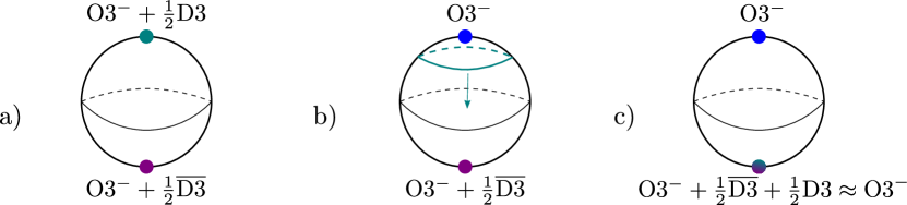
Figure 4: Non-perturbative decay process into the supersymmetric configuration. a) The original configuration with a nilpotent Goldstino. We display the $S^{3}/\mathbb{Z}_{2}$ at the bottom of the throat. b) We resolve the stuck D3-brane into a D5 wrapping $\mathbb{RP}^{2}\in S^{3}/\mathbb{Z}_{2}$. c) We close the $\mathbb{R}\mathbb{P}^{2}$ over the other orientifold fixed point, and tachyon condensation takes over, rolling down to the supersymmetric vacuum.

If we adapt this discussion to the case of the two O3-planes at the bottom of the cascade with stuck D3 and $\overline{\rm{D3}}$ branes, we have that we can resolve the stuck D3-brane (say) into a D5-brane wrapping the $\mathbb{R}\mathbb{P}^{2}$ at the equator of the $S^{3}/\mathbb{Z}_{2}$ at the bottom of the cascade, and then close this D5 on the other side of the $S^{3}/\mathbb{Z}_{2}$, where the $\overline{\rm{D3}}$ is stuck. The resulting system has an ordinary O3^- on one fixed point on the $S^{3}/\mathbb{Z}_{2}$, and a D3-$\overline{\rm{D3}}$ pair stuck on top of the other O3^-. The brane-antibrane pair can then annihilate by ordinary tachyon condensation, and we return to the original supersymmetric vacuum. We show the process in figure 4.

4 Global embeddings

Now that we understand the local dynamics in detail, let us try to construct a global example exhibiting these dynamics. The conifold singularity is ubiquitous in the space of Calabi-Yau compactifications. It is, however, less easy to find a space that admits the involution described above and allows for the cancellation of all tadpoles.

We may try to find global embeddings on the “resolution phase”, or on the “deformation phase”. In the first case, we try to construct a toric space such that is has a conifold singularity admitting the desired involution. The simplest construction would have the conifold realised as a face of the toric polytope, as in Balasubramanian:2012wd . These are ubiquitous, as discussed in that paper. One should then search the subclass of models compatible with an involution of the form (22).

We can instead choose to search for models in the “deformation phase”, namely directly on the side described by flux and a $S^{3}$ with O3-planes at the north and south poles of a deformed conifold, which is the description of interest for model building. In this paper we focus on models directly described in the deformation phase, leaving the search for models in the resolution phase for future work.

A possible search strategy is as follows: first we construct consistent type IIB models with O3-planes in them. We choose to construct them by giving a Calabi-Yau threefold, and specifying an appropriate involution on it. Then we try to deform the complex structure such that two O3-planes are brought together. If this is possible, we analyze the topology of the resulting Calabi-Yau (before taking the involution) to see whether the neighborhood of the points where the O3 planes coincide is locally a conifold. If so, we need to verify whether tadpoles can be cancelled. This is the way we found one of our two examples, that we describe in §4.2. An exhaustive search may produce several candidates. We leave this for future work.

In our first example, however, we present a variation of this strategy. One can construct some (non-Calabi-Yau) base $\mathcal{B}$, with some interesting properties to be discussed momentarily, over which we fibre a torus in such a way that we obtain a Calabi-Yau fourfold. We then take the F-theory limit in order to produce the desired type IIB background. The defining property of $\mathcal{B}$ is that it has one or more (deformed) conifold singularities, and that the local involution (19) extends to an involution $\sigma$ over $\mathcal{B}$. The fourfold of interest will then be a Calabi-Yau genus one fibration over $\mathsf{B}=\mathcal{B}/\sigma$. Over the fixed points in $\mathsf{B}$ we will find a local structure of the form $\mathbb{C}^{3}/\mathbb{Z}_{2}$, with the $\mathbb{Z}_{2}$ acting as $(x,y,z)\to(-x,-y,-z)$, which is not Calabi-Yau. The Calabi-Yau fourfold will then promote this local structure to four terminal $\mathbb{C}^{4}/\mathbb{Z}_{2}$ singularities, which signal the appearance of an O3.

These conditions on $\mathcal{B}$ do not seem very restrictive, so we expect to be able to find examples with relative ease. We again leave a systematic classification for the future. Here we present a simple example of this sort, that we now discuss.

4.1 F-theory construction

One early well-known example of conifold embedding in the string phenomenology literature already exhibits the structure we want Giddings:2001yu . Take $\mathcal{B}$ to be defined by a quartic on $\mathbb{P}^{4}$ of the form

$$P=\sum_{i=1}^{4}(z_{5}^{2}+z_{i}^{2})z_{i}^{2}-t^{2}z_{5}^{4}=0\,.$$ (66)

We have intentionally abused notation, and denoted the projective coordinates of $\mathbb{P}^{4}$ by $z_{1},\ldots,z_{5}$, similarly to a set of coordinates used for the conifold above. As in Giddings:2001yu , we choose $t$ to be real. It is then easily checked that $\mathcal{B}$ is smooth for $t\neq 0$, but develops a conifold singularity at $[0:0:0:0:1]$ when $t=0$. In a neighborhood of this point we can gauge-fix $z_{5}=1$, obtaining a local structure

$$\widetilde{P}=\sum_{i=1}^{4}(1+z_{i}^{2})z_{i}^{2}-t^{2}=0$$ (67)

which for small enough $z_{i}$ is the standard form of the conifold.

The involution (36) is then clearly extensible to $\mathcal{B}$, by taking

$$\sigma\colon(z_{1},z_{2},z_{3},z_{4},z_{5})\to(-z_{1},z_{2},-z_{3},-z_{4},z_{5})\,.$$ (68)

The fixed loci are at $z_{1}=z_{3}=z_{4}=0$ and $z_{2}=z_{5}=0$. (We will later blow-up the latter). The first set consists of four points in $\mathcal{B}$, given by the solutions of $(z_{5}^{2}+z_{2}^{2})z_{2}^{2}-t^{2}z_{5}^{4}$. In all four points we need to have $z_{5}\neq 0$ (otherwise $z_{1}=\ldots=z_{5}=0$, which is not in $\mathbb{P}^{4}$). Gauge fixing $z_{5}=1$ again, the four fixed points are at the solutions of $(1+z_{2}^{2})z_{2}^{2}=t^{2}$. As we send $t\to 0$, two of these fixed points go into the singularity, while the other two stay at finite distance, at $z_{2}^{2}+1=0$.

If we take the quotient of the described manifold by the involution (68), we would get the local structure we want around the shrinking $S^{3}$, but we would have a slightly strange behavior around the other fixed point locus, i.e. the one at $z_{2}=z_{5}=0$. In fact, this would be a codimension-2 orientifold locus, which is unconventional in compactifications with O3-planes. For this reason we slightly change the base manifold, by blowing up $\mathbb{P}^{4}$ along $z_{2}=z_{5}=0$. We then obtain a toric ambient space described by the following GLSM

$$\begin{array}[]{c|cccccc}&z_{1}&z_{2}&z_{3}&z_{4}&z_{5}&\lambda\\ \hline\cr\mathbb{C}^{*}_{1}&1&1&1&1&1&0\\ \mathbb{C}^{*}_{2}&1&0&1&1&0&1\end{array}$$ (69)

with SR-ideal $\{z_{1}z_{3}z_{4}\lambda,z_{2}z_{5}\}$. Now $z_{2}z_{5}$ is in the SR-ideal, i.e. the unwanted codimension-2 fixed point locus does not exist anymore. On the other hand, there is now a codimension-1 fixed point locus, i.e. $\lambda=0$. The base equation is now

$$\hat{P}=\sum_{i=1,3,4}(z_{5}^{2}\lambda^{2}+z_{i}^{2})z_{i}^{2}+(z_{5}^{2}+z_{2}^{2})z_{2}^{2}\lambda^{4}-t^{2}z_{5}^{4}\lambda^{4}=0\,.$$ (70)

It again restricts to (67) around the conifold singularity (when $t=0$). Notice that the fixed points $z_{1}=z_{3}=z_{4}=0$ are far away from the codimension-1 fixed point locus $\lambda=0$. Moreover, the involution can now be given by $\lambda\mapsto-\lambda$ (due to the scaling relations).

In order to describe $\mathsf{B}=\mathcal{B}/\sigma$, with $\sigma\colon\lambda\mapsto-\lambda$, we introduce the invariant coordinate $\Lambda=\lambda^{2}$. Our new base is now a complete intersection in the ambient space described by

$$\begin{array}[]{c|cccccc}&z_{1}&z_{2}&z_{3}&z_{4}&z_{5}&\Lambda\\ \hline\cr\mathbb{C}^{*}_{1}&1&1&1&1&1&0\\ \mathbb{C}^{*}_{2}&1&0&1&1&0&2\end{array}$$ (71)

with SR-ideal $\{z_{1}z_{3}z_{4}\Lambda,z_{2}z_{5}\}$. This is a two-to-one map from the previous base, except on the fixed loci $\lambda=0$ and $z_{1}=z_{3}=z_{4}=0$, where it is one-to-one. The defining equation is $\mathsf{P}=0$ where $\mathsf{P}$ comes from (70):

$$\mathsf{P}=\sum_{i=1,3,4}(z_{5}^{2}\Lambda+z_{i}^{2})z_{i}^{2}+(z_{5}^{2}+z_{2}^{2})z_{2}^{2}\Lambda^{2}-t^{2}z_{5}^{4}\Lambda^{2}=0\,.$$ (72)

As an example, consider a neighborhood of the fixed points at $z_{1}=z_{3}=z_{4}=0$. We necessarily have $\Lambda\neq 0$ and $z_{5}\neq 0$ (otherwise at $\mathsf{P}=0$ we would have $z_{5}=z_{2}=0$). We can thus gauge fix $\Lambda=1$ and $z_{5}=1$, which leaves

$$\widetilde{\mathsf{P}}=\sum_{i=1,3,4}(1+z_{i}^{2})z_{i}^{2}+(z_{2}^{2}+1)z_{2}^{2}-t^{2}=0$$ (73)

and a $\mathbb{Z}_{2}$ inverting the $z_{1},z_{3},z_{4}$ coordinates. So we are left with precisely the quotient of the deformed conifold that we had locally.

We now uplift this configuration to F-theory. We choose the standard Weierstrass model: a genus-one fibration with a section, with the fibre realised as a degree six hypersurface on $\mathbb{P}^{2,3,1}$. Notice that the base has first Chern class $c_{1}(\mathsf{B})=[z_{1}]$. The CY four-fold will be a complete intersection on a an ambient toric space $\mathcal{A}$ given by the GLSM

$$\begin{array}[]{c|ccccccccc}&z_{1}&z_{2}&z_{3}&z_{4}&z_{5}&\Lambda&x&y&z\\ \hline\cr\mathbb{C}^{*}_{1}&1&1&1&1&1&0&0&0&-1\\ \mathbb{C}^{*}_{2}&1&0&1&1&0&2&0&0&-1\\ \mathbb{C}^{*}_{3}&0&0&0&0&0&0&2&3&1\end{array}$$ (74)

where we took the coordinate $z$ to belong to the anticanonical bundle of $\mathsf{B}$. The degree six equation will be given by

$$\mathsf{Q}=x^{3}+f(z_{i},\Lambda)xz^{4}+g(z_{i},\Lambda)z^{6}-y^{2}=0$$ (75)

with $f,g$ homogeneous polynomials of the base coordinates of degrees $(4,4)$ and $(6,6)$ respectively.

At this point we can do a couple of sanity checks of our construction:

1. The neighborhood of the O3-planes on the contracting $S^{3}$ should look like an elliptic fibration over $\mathbb{C}^{3}/\mathbb{Z}_{2}$ (with a fixed point) with monodromy in the fibre given by $-1\in SL(2,\mathbb{Z})$. In particular, it should be the case that generically $\Delta=0$ does not intersect the location of the O3-planes. But there should be, at any fixed point in the base corresponding to an O3, an involution of the $T^{2}$ sending $q\to-q$ (with $q$ the flat coordinate in the $T^{2}$).

2. Relatedly, $\Delta=0$ should not intersect the conifold point in the base if we send $t\to 0$, so the local system is the one we wanted to embed originally.

We now perform these sanity checks. We work directly in the limit $t=0$. If we find that $\Delta\neq 0$ at the conifold point this will imply that for finite $t$ there is no intersection with the fixed points either (this second fact can also be checked easily independently for $t\neq 0$, but we will not do so explicitly here). When $t=0$, the conifold fixed point $\mathcal{P}_{c}$, where the two O3 planes come on top of each other, is at $(z_{1},z_{2},z_{3},z_{4},z_{5})=[0\colon 0\colon 0\colon 0\colon 1]$. A generic degree $(4,4)$ section (such as $f$) restricted to $\mathcal{P}_{c}$ has the form

$$f|_{\mathcal{P}_{c}}=f_{0}z_{5}^{4}\Lambda^{2}=f_{0}$$ (76)

with generically $f_{0}\neq 0$. So we learn that $f\neq 0$ at the fixed points. A similar argument for $g$ gives $g|_{\mathcal{P}_{c}}\neq 0$, and generically also $\Delta|_{\mathcal{P}_{c}}=4f_{0}^{3}+27g_{0}^{2}\neq 0$ for generic $f_{0}$ and $g_{0}$. So we learn that the discriminant does not intersect the O3-planes. Furthermore, the argument is independent of the value of $t$, so the discriminant locus does not intersect the conifold singularity either, and locally we just have the type IIB system of interest. This is as expected, since locally we have a O3 involution of a Calabi-Yau, which can be realised supersymmetrically at constant $\tau$, so there is no need to have 7-branes to restore supersymmetry.

Let us look at the structure around a fixed point at $z_{1}=z_{3}=z_{4}=0$. As discussed above, we can fix $\Lambda=1$ and $z_{5}=1$. This leaves a $\mathbb{Z}_{2}$ symmetry acting as $z\to-z$, leaving all other non-zero coordinates invariant. Choose a root for $\widetilde{P}=(z_{2}^{2}+1)z_{2}^{2}-t^{2}$. This leaves us with the fibre, as expected, quotiented by a $\mathbb{Z}_{2}$ acting as

$$\widehat{\sigma}\colon(x,y,z)\to(x,-y,z)\,.$$ (77)

(We have used the $\mathbb{P}^{2,3,1}$ $\mathbb{C}^{*}$ to make the sign act on $y$, instead of $z$.) In terms of the flat coordinate $q$ on the torus we have $x=\wp(q)$ and $y=\wp^{\prime}(q)$, using the Weierstrass $\wp$-function. Since $\wp(q)$ is even on $q$, and thus $\wp^{\prime}(q)$ odd, we can identify the $\mathbb{Z}_{2}$ action (77) precisely as $q\to-q$, or in terms of IIB variables $(-1)^{F_{L}}\Omega$.

We are now going to consider the weak coupling limit, to extract a Calabi-Yau three-fold with the wanted involution and properties. We will also consider the simple situation in which the D7-brane tadpole is canceled locally Sen:1996vd . We then have $f=\phi\,h^{2}$ and $g=\gamma\,h^{3}$ where $\phi,\gamma$ are constant and $h$ is a polynomial of degree $(2,2)$ in $z_{i},\Lambda$. Its most generic form is

$$h(z_{i},\Lambda)\equiv\Lambda\,p_{2}(z_{2},z_{5})+q_{2}(z_{1},z_{3},z_{4})\>,$$ (78)

where $p_{2},q_{2}$ are polynomials of degree 2. The Calabi-Yau three-fold is then given by adding the equation $\xi^{2}=h$, i.e.

$$\xi^{2}=\Lambda\,p_{2}(z_{2},z_{5})+q_{2}(z_{1},z_{3},z_{4})\qquad{\rm AND}\qquad\mathsf{P}=0$$ (79)

in the ambient space

$$\begin{array}[]{c|ccccccc}&z_{1}&z_{2}&z_{3}&z_{4}&z_{5}&\Lambda&\xi\\ \hline\cr\mathbb{C}^{*}_{1}&1&1&1&1&1&0&1\\ \mathbb{C}^{*}_{2}&1&0&1&1&0&2&1\end{array}$$ (80)

with SR-ideal $\{z_{2}z_{5},\,\,z_{1}z_{3}z_{4}\Lambda\xi\}$. From (79) we see that we have one O7-plane at $\xi=0$.

The intersection form on the 5-fold ambient space is computed in the following way. Let us first take the basis $D_{1}=D_{z_{1}}$ and $D_{2}=D_{z_{2}}$. We moreover observe that we have one point at $(z_{1},z_{2},z_{3},z_{4},z_{5},\Lambda,\xi)=(0,0,0,0,1,0,1)$, i.e. $H_{1}^{4}(2H_{1}-2H_{2})=1$. The SR-ideal tells us that $H_{2}^{2}=0$ and $H_{1}^{4}(H_{1}-H_{2})=0$. Hence we obtain that the only two non-vanishing intersection numbers are $H_{1}^{5}=H_{1}^{4}H_{2}=\frac{1}{2}$. Hence on the CY three-fold, that is defined by intersecting the two divisors in the classes $[P]=4H_{1}$ and $[\xi^{2}]=2H_{1}$, we have the intersection form

$$I_{3}=4D_{1}^{3}+4D_{1}^{2}D_{2}\>.$$ (81)

We can also compute the second Chern class of the three-fold by adjunction. We obtain

$$c_{2}(X_{3})=6D_{1}^{2}+4D_{1}D_{2}\>.$$ (82)

For our purposes, the important equation is $\mathsf{P}=0$ that gives the conifold singularity and the physics we are interested in. One can easily see that in the double cover description we indeed have a conifold singularity (as opposed to its quotient). To see this, zoom on the neighborhood of $z_{1}=z_{3}=z_{4}=0$. Looking to the expression (78), we see that on the $z_{1}=z_{3}=z_{4}=0$ locus $\Lambda=0$ implies $\xi=0$, so given that $z_{1}z_{3}z_{4}\Lambda\xi$ belongs to the SR-ideal, we conclude that in this neighborhood, for generic $p_{2}(z_{2},z_{5})$, $\Lambda\neq 0$. We can thus gauge fix $\Lambda=1$, which leaves a $\mathbb{Z}_{2}$ subgroup unfixed. This subgroup is precisely the one that exchanges the two roots of $\xi^{2}=h$, so we can gauge fix it by choosing arbitrarily one of the roots in the whole neighborhood. As above, due to the $\mathsf{P}=0$ equation and the fact that $z_{2}z_{5}$ belongs to the SR-ideal, we have that $z_{5}\neq 0$, so we can use it to gauge-fix the remaining $\mathbb{C}^{*}$ symmetry by setting $z_{5}=1$. We thus end up with $\widetilde{P}(z_{1},z_{2},z_{3},z_{4})=0$, as in (73), i.e. a deformed conifold singularity with no quotient acting on it.

We can also compute the Euler characteristic of the O7-plane divisor, that allows us to compute the D3-charge of the O7-plane and four D7-branes (plus their images) on top of it. In fact we have $[O7]=H_{1}$. The Euler characteristic of a four-cycle $D$ is

$$\chi(D)=\int_{D}c_{2}(D)=\int_{X_{3}}D(D^{2}+c_{2}(X))\>,$$ (83)

where in the last step we used the adjunction formula (to obtain $c_{2}(D)=c_{1}(D)^{2}+c_{2}(X)$) and the fact that $D$ is a divisor of a CY (and then $c_{1}(D)=-D$). In our case $\chi([O7])=H_{1}^{3}+H_{1}c_{2}(X)=44$. Hence the geometric induced D3-charge of the system made up of the O7-plane plus four D7-branes (plus their images) on top of it is

$$Q_{D3}^{(4D7+O7)}=-\frac{\chi([O7])}{2}=-22\>.$$ (84)

Any half-integral flux (that could be induced by the Freed-Witten anomaly cancellation condition) gives an integral contribution in this configuration (since there are eight D7-branes).

One further thing to check is whether there are constraints on the NSNS three-form flux coming from the Freed-Witten anomaly Witten:1998xy ; Freed:1999vc . These will be absent if $H^{3}(O7,\mathbb{Z})=0$. This follows from the Lefschetz hyperplane theorem as follows. We start by desingularising the ambient toric space (80). The singularity is at $z_{1}=z_{3}=z_{4}=\xi=0$. It can be easily seen that this locus does not intersect the Calabi-Yau hypersurface, for generic $p_{2},q_{2}$. So if we blow up along the singular point we do not alter the Calabi-Yau itself (or any of its divisors). A possible desingularised ambient space is

$$\begin{array}[]{c|cccccccc}&z_{1}&z_{2}&z_{3}&z_{4}&z_{5}&\Lambda&\xi&s\\ \hline\cr\mathbb{C}^{*}_{1}&1&1&1&1&1&0&1&0\\ \mathbb{C}^{*}_{2}&1&0&1&1&0&2&1&0\\ \mathbb{C}^{*}_{3}&0&0&0&0&0&1&0&1\end{array}$$ (85)

with SR-ideal $\{z_{2}z_{5},s\Lambda,z_{1}z_{3}z_{4}\xi\}$. The locus of interest is given by

$$\{\xi=0\}\quad\cap\quad\{s\xi^{2}=\hat{h}\}\quad\cap\quad\{\hat{P}=0\}$$ (86)

with

$$\hat{P}=\sum_{i=1,3,4}(z_{5}^{2}\Lambda+sz_{i}^{2})sz_{i}^{2}+(z_{5}^{2}+z_{2}^{2})z_{2}^{2}\Lambda^{2}-t^{2}z_{5}^{4}\Lambda^{2}$$ (87)

and

$$\hat{h}=\Lambda p_{2}(z_{2},z_{5})+sq_{2}(z_{1},z_{3},z_{4})$$ (88)

the proper transforms of the original divisors. We start by imposing $\xi=0$. This gives rise to a toric space $\mathcal{A}_{\xi}$ of one dimension lower, which can easily be seen to be smooth. Similarly, $\hat{h}=0$ gives rise to a smooth hypersurface $Y$ in $\mathcal{A}_{\xi}$, and it can be seen that the O7 locus $\hat{P}=0\subset Y$ is also smooth. So by straightforward repeated application of the Lefschetz hyperplane theorem we learn that $H_{1}(O7,\mathbb{Z})=H_{1}(\hat{\mathcal{A}},\mathbb{Z})$, with $\hat{\mathcal{A}}$ the ambient toric space (85). But it is easy to see that $\pi_{1}(\hat{\mathcal{A}})=0$ from standard considerations in toric geometry (see for instance theorem 12.1.10 in cox2011toric ), so by the Hurewicz isomorphism and Poincaré duality on the O7 worldvolume we learn that $H^{3}(O7,\mathbb{Z})=0$.

4.2 Goldstino retrofitting

The model in the previous section was designed in order to display the structure of interest. While this is interesting, it is also interesting to see if existing, phenomenologically interesting type IIB models with O3-planes admit the addition of a nilpotent Goldstino sector, “retrofitting” them with a possible de Sitter uplift mechanism at little cost.

To show that this is indeed the case, we consider the model in Diaconescu:2007ah ; Cicoli:2012vw . It is constructed starting from a hypersurface in the toric ambient space

$$\begin{array}[]{c|cccccccc|c}&W_{1}&W_{2}&W_{3}&W_{4}&W_{5}&Z&X&Y&D_{\textmd{H}}\cr\hline\cr\mathbb{C}_{1}^{*}&0&0&0&0&0&1&2&3&6\cr\mathbb{C}_{2}^{*}&1&1&1&0&0&0&6&9&18\cr\mathbb{C}_{3}^{*}&0&1&0&1&0&0&4&6&12\cr\mathbb{C}_{4}^{*}&0&0&1&0&1&0&4&6&12\cr\end{array}\,,$$ (89)

with SR-ideal

$${\rm SR}=\{W_{1}\,W_{2}\,W_{3},\,W_{2}\,W_{4},\,W_{3}\,W_{5},\,W_{4}\,W_{5},\,W_{1}\,W_{2}\,X\,Y,\,W_{1}\,W_{3}\,X\,Y,\,W_{4}\,Z,\,W_{5}\,Z,\,X\,Y\,Z\}\,.$$ (90)

The last column indicates the degree of the polynomial defining the CY three-fold. This polynomial takes the form of a Weierstrass model

$$Y^{2}=X^{3}+f(W_{i})\,X\,Z^{4}+g(W_{i})\,Z^{6}\>,$$ (91)

where $f$ and $g$ are respectively polynomials of degree $(0,12,8,8)$ and $(0,18,12,12)$ in the coordinates $W_{1},\ldots,W_{5}$.

This CY $X$ has Hodge numbers $h^{1,1}=4$ and $h^{1,2}=214$. The intersection form takes the simple expression

$$I_{3}=9D_{1}^{3}+D_{2}^{3}+D_{3}^{3}+9D_{4}^{3}$$ (92)

in the following basis of $H^{1,1}(X)$:

$$D_{1}=3D_{W_{3}}+3D_{W_{4}}+D_{Z}\qquad D_{2}=D_{W_{4}}\qquad D_{3}=D_{W_{5}}\qquad D_{4}=D_{Z}\>.$$ (93)

Three of the basis elements are del Pezzo surfaces. In particular $\{Z=0\}$ is a $dP_{0}$, while $\{W_{4}=0\}$ and $\{W_{5}=0\}$ are $dP_{8}$’s. The second Chern class of the Calabi-Yau is

$$c_{2}(X_{3})=\frac{1}{3}\left(34D_{1}^{2}+30D_{2}^{2}+30D_{3}^{2}-2D_{4}^{2}\right)\>.$$ (94)

We consider the involution Diaconescu:2007ah ; Cicoli:2012vw

$$W_{2}\leftrightarrow W_{3}\qquad\mbox{and}\qquad W_{4}\leftrightarrow W_{5}$$ (95)

exchanging the two $dP_{8}$’s. The CY three-fold equation must be restricted to be invariant under this involution. $X,Y,Z$ are invariant under such involution. The rest of invariant monomials are $W_{1}$, $u\equiv W_{2}W_{3}$, $v\equiv W_{4}W_{5}$ and $w\equiv W_{3}W_{4}+W_{2}W_{5}$. The equation becomes invariant if $f$ and $g$ depend on $W_{i}$ only as functions of $W_{1},u,v,w$.

Let us consider the fixed point locus. It is made up of a codimension-1 locus at $W_{3}W_{4}-W_{2}W_{5}=0$ and four isolated fixed points: one at the intersection $W_{3}W_{4}+W_{2}W_{5}=W_{1}=Z=0$ and three at the intersection $W_{3}W_{4}+W_{2}W_{5}=W_{1}=Y=0$ Diaconescu:2007ah ; Cicoli:2012vw . So by implementing this orientifold involution, one obtains one O7-plane in the class $[D_{O7}]=[D_{W_{3}}]+[D_{W_{4}}]$ and four O3-planes.

We focus on the neighborhood of the O3-planes at $Y=W_{1}=w=0$ (we have used the above definition $w\equiv W_{3}W_{4}+W_{2}W_{5}$). If we plug these relations inside the defining equation (91), we get a cubic in X

$$X^{3}+\alpha Xu^{6}v^{2}Z^{4}+\beta u^{9}v^{3}Z^{6}=0$$ (96)

where, as said above, $f$ and $g$ are functions of the invariant monomials, and $\alpha,\beta$ are tunable complex structure moduli. First of all, because of SR-ideal, we know that $u$, $v$ and $Z$ are non-vanishing. We can thus fix $W_{4}=W_{5}=Z=1$ and $W_{2}=i$ via the projective rescalings, in which case $W_{3}W_{4}+W_{2}W_{5}=0$ becomes simply $W_{3}=-i$. In terms of the invariant coordinates we have $u=v=1$. With this gauge choice we have that (96) becomes

$$X^{3}+\alpha X+\beta=0\,.$$ (97)

Hence the zeros of (96) are at the zeros of the cubic equation. We are interested to the case when two of these zeros come together. This happens when the discriminant of the cubic is zero, i.e. when

$$\Delta\equiv 4\alpha^{3}+27\beta^{2}=0\>,$$ (98)

that is a relation among the complex structure parameters. We can parametrise this situation by taking $\alpha=-3a^{2}$ and $\beta=2a^{3}-\delta$. When $\delta=0$ two of the roots come together. We can also rewrite the cubic equation as

$$(X-a)^{2}(X+2a)-\delta=0\>.$$ (99)

Now it is manifest that when $\delta=0$ we have a double root at $X=a$.

Let us study the local form of (91) around $Y=W_{1}=w=X-a=0$. As above, we use the $\mathbb{C}^{*}$ symmetries to fix $W_{4}=W_{5}=Z=1$. In addition, we gauge fix $u=1$. Notice that this leaves an unfixed $\mathbb{Z}_{2}$ subgroup, generated by $(\lambda_{1},\lambda_{2},\lambda_{3},\lambda_{4})=(1,-1,1,1)$. We choose to fix this subgroup by requiring that at the fixed point $W_{2}=i$, as above, or in terms of coordinates on a neighborhood of the point, that $W_{2}=i+\omega-\frac{i}{2}\omega^{2}$, with $|\omega|\ll 1$. To quadratic order in $\omega$ this gauge fixing implies $W_{3}=W_{2}^{-1}=-i+\omega+\frac{i}{2}\omega^{2}$. Expanding in terms of these new coordinates around $Y=W_{1}=w=X-a=0$ we have

$$-Y^{2}+(X-a)^{2}(3a+\ldots)+W_{1}^{2}(c_{W_{1}}+\ldots)+\omega^{2}(c_{\omega}+\ldots)=\delta$$ (100)

where $\ldots$ are terms that vanish on the analysed locus and $c_{W_{1}}$ and $c_{w}$ are generically non zero constants (in the chosen patch). We have used the freedom in redefining the complex coordinates in order to erase possible $W_{1}\omega$ mixed terms. We immediately see that we obtain a conifold singularity when $\delta\rightarrow 0$.

How does the permutation involution act on this local conifold? The coordinates $X,Y,Z,u,v$ are all invariant, as is the gauge fixing $Z=W_{4}=W_{5}=u=1$. On the other hand, the image of $(W_{2},W_{3})=(i+\omega-\frac{i}{2}\omega^{2},-i+\omega+\frac{i}{2}\omega^{2})$ is $(W_{2},W_{3})=(-i+\omega+\frac{i}{2}\omega^{2},i+\omega-\frac{i}{2}\omega^{2})$, which is not in the form given by the $\mathbb{Z}_{2}$ gauge fixing above. We can go back to the desired gauge frame by acting with $\lambda_{2}=-1$, which acts on our local conifold coordinates as

$$(X-a,Y,W_{1},\omega)\mapsto(X-a,-Y,-W_{1},-\omega)$$ (101)

and perfectly reproduces the geometric action required for the retrofitting of a nilpotent Goldstino sector.

Let us finish with some considerations on the D3-charge. Remember first that we have four O3-planes. The D3-charge of the system of the O7-plane and four D7-branes (plus their images) on top of it, is given by $-\chi([O7])/2$, where $[O7]$ is the homology class of the O7-plane locus. In our case $[O7]=D_{W_{3}}+D_{W_{4}}=\frac{1}{3}(D_{1}-D_{4})$. By using (94), the Euler characteristic can be computed, as $\chi(D)=D^{3}+c_{2}(X_{3})D$ in a CY three-fold. We obtain $\chi([O7])=36$. Hence the localised objects in the compactification have integral D3-charge. As discussed in §3.5, choose for instance to put a stuck D3 at one of the O3^- points on the contracting $S^{3}$, and a stuck $\overline{\rm{D3}}$ on the other O3^- on this same $S^{3}$. This pair of stuck branes does not contribute to the D3 tadpole. Finally, recall that we introduce fractional branes in the orientifolded conifold cascade in order to create the warped throat by confinement. The number of branes to introduce is arbitrarily tunable, and completely determines the amount of D3 charge induced by the fluxes in the confined description, i.e. threading the warped throat.

5 Conclusions

We have presented the first explicit CY compactifications with anti-D3-branes at the tip of a long throat for which the single propagating degree of freedom is the goldstino and therefore can be represented by a nilpotent superfield.

Anti-D3-branes are an important tool for type IIB phenomenology. An anti-D3-brane at the tip of a warped throat, generated by three-form fluxes Giddings:2001yu , produces an uplifting term to the scalar potential, that allows to obtain de Sitter minima Kachru:2003aw . By a mild tuning of the three-form fluxes, one can get a fine tuning of the cosmological constant, that is model independent if the throat is localised far from the visible spectrum. The presence of the anti-D3-brane can be described in a supersymmetric effective field theory (even if non-linearly) by the introduction of constrained superfields. The simplest situation is when the anti-D3-brane is on top of an O3-plane at the tip of the throat: one needs just to add one nilpotent superfield that captures the goldstino degrees of freedom. This has been studied in Kallosh:2015nia .

In this paper we have discussed how to realise this setup in a globally consistent Calabi-Yau compactification. The necessary ingredients are a warped throat, realised by considering a KS deformed conifold throat embedded in a compact CY like in Giddings:2001yu , and an orientifold involution that produces a couple of O3-planes at the tip of the throat.

We first analysed the local neighbourhood of the O3/$\overline{\rm{D3}}$ system. We started from considering the conifold singularity. It is well know that putting three-form fluxes on the deformed conifold produces a warped throat with a three-sphere at the tip. This three-sphere collapses when the deformation goes to zero and the conifold singularity is generated. We have first studied the situation for the singular conifold and then transported our result to the deformed one. We have considered the simplest involution that keeps the singularity fixed. This involution has no fixed points in the resolved phase (although this statement is somewhat subtle due to the fact that the geometric resolution mode is projected out, as we have explained), but has still two fixed points on the deformed phase, that are placed on the north and south poles of the three-sphere at the tip of the throat. These two fixed points collapse on top of each other when one takes the singular limit. Hence, by using this orientifold involution in the deformed phase, one generates two O3-planes at the tip of the throat. We also mapped the system to the T-dual type IIA configuration, that is well known also in the orientifolded case. This allowed us to double check some of our conclusions and solve some apparent puzzles.

For the unorientifolded KS throat it is well known that the deformed phase is realised dynamically in the field theory living on a stack of D3-branes probing the conifold singularity: the classical moduli space is deformed quantum mechanically due to the dynamically generated F-terms. The same process takes place in the orientifolded case, and by a careful analysis of the quantum dynamics of the $SO\times U\!Sp$ theory at the singularity we have determined which type of O3-plane is generated. We have found agreement with the prediction from the type IIA dual configuration: the two O3-planes are of the same type, either both $O3^{-}$ for $U\!Sp$ confinement (with one or both of type $\widetilde{O3}^{-}$), or both $O3^{+}$ for $SO$ confinement.

We have used the local results outlined above to embed the system in a compact CY. We have found two examples. In both cases, we have constructed a CY three-fold with the following properties: 1) It has a definite complex structure deformation that allows to take the explicit conifold limit, i.e. we have identified a parameter in the CY defining equation that generates a conifold singularity when set to zero. 2) It has an involution that, in the local patch around the conifold singularity (or the tip of the deformed one), acts in the same way we found in the local analysis and that gives two O3-planes on top of the deformed conifold three-sphere. We have followed two procedures to find our compact examples. In the first case we constructed the CY, by first embedding the orientifolded conifold in a non-Calabi-Yau compact threefold. Then, by constructing a F-theory model over this base and taking its Sen weak coupling limit, we have constructed a CY three-fold with the wanted features. In the second case, we started with a previously studied phenomenologically interesting CY with an involution that generates more than one O3-plane and then checked that there is a deformation of the defining equation that brings two O3-planes on top of each other. We showed that this deformation generates a conifold singularity on the point where the two O3-planes coincide. It would be interesting to systematise both methods (direct construction and search) to obtain a list of suitable CYs.

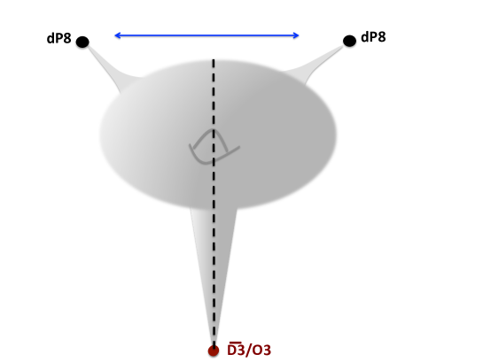
Figure 5: CY manifold of §4.2, when two dP₈ divisors are shrunk to zero size to generate two singularities (exchanged by orientifold involution). D3-branes on these singularities produce non-abelian gauge groups and chiral spectrum.

In summary, we have achieved the concrete construction of simple models satisfying all requirements for a proper global embedding of the $\overline{\rm{D3}}$ at the tip of a throat with the nilpotent goldstino in the spectrum. One can extend our results to present explicit calculations for moduli stabilisation for both KKLT Kachru:2003aw and Large Volume (LVS) Balasubramanian:2005zx ; Conlon:2005ki scenarios. The CY manifold in §4.2 and the studied involution was used in Cicoli:2012vw to realise a type IIB global model with chiral spectrum coming from D3-branes at dP₈ singularities (these are realised by shrinking the four-cycles $D_{W_{4}}$ and $D_{W_{5}}$) and with all geometric moduli stabilised. In that paper the dS uplift was meant to be induced by a T-brane Cicoli:2015ylx , but here we have shown that also the anti-D3-brane uplift may be realised. See figure 5 for a picture of the setup. We will study this example in detail in a future work.

- (1) E. A. Bergshoeff, D. Z. Freedman, R. Kallosh and A. Van Proeyen, Pure de Sitter Supergravity, Phys. Rev. D92 (2015) 085040, [1507.08264].
- (2) E. Dudas, S. Ferrara, A. Kehagias and A. Sagnotti, Properties of Nilpotent Supergravity, JHEP 09 (2015) 217, [1507.07842].
- (3) I. Antoniadis and C. Markou, The coupling of Non-linear Supersymmetry to Supergravity, Eur. Phys. J. C75 (2015) 582, [1508.06767].
- (4) F. Hasegawa and Y. Yamada, Component action of nilpotent multiplet coupled to matter in 4 dimensional supergravity, JHEP 10 (2015) 106, [1507.08619].
- (5) R. Kallosh and T. Wrase, De Sitter Supergravity Model Building, Phys. Rev. D92 (2015) 105010, [1509.02137].
- (6) G. Dall’Agata, S. Ferrara and F. Zwirner, Minimal scalar-less matter-coupled supergravity, Phys. Lett. B752 (2016) 263–266, [1509.06345].
- (7) M. Schillo, E. van der Woerd and T. Wrase, The general de Sitter supergravity component action, in 21st European String Workshop: The String Theory Universe Leuven, Belgium, September 7-11, 2015, 2015. 1511.01542.
- (8) R. Kallosh, A. Karlsson and D. Murli, From Linear to Non-linear Supersymmetry via Functional Integration, 1511.07547.
- (9) R. Kallosh and T. Wrase, Emergence of Spontaneously Broken Supersymmetry on an Anti-D3-Brane in KKLT dS Vacua, JHEP 12 (2014) 117, [1411.1121].
- (10) E. A. Bergshoeff, K. Dasgupta, R. Kallosh, A. Van Proeyen and T. Wrase, and dS, JHEP 05 (2015) 058, [1502.07627].
- (11) R. Kallosh, F. Quevedo and A. M. Uranga, String Theory Realizations of the Nilpotent Goldstino, 1507.07556.
- (12) L. Aparicio, F. Quevedo and R. Valandro, Moduli Stabilisation with Nilpotent Goldstino: Vacuum Structure and SUSY Breaking, 1511.08105.
- (13) I. Bandos, L. Martucci, D. Sorokin and M. Tonin, Brane induced supersymmetry breaking and de Sitter supergravity, 1511.03024.
- (14) S. Kachru, R. Kallosh, A. D. Linde and S. P. Trivedi, De Sitter vacua in string theory, Phys. Rev. D68 (2003) 046005, [hep-th/0301240].
- (15) S. B. Giddings, S. Kachru and J. Polchinski, Hierarchies from fluxes in string compactifications, Phys. Rev. D66 (2002) 106006, [hep-th/0105097].
- (16) P. Candelas and X. C. de la Ossa, Comments on Conifolds, Nucl. Phys. B342 (1990) 246–268.
- (17) I. R. Klebanov and E. Witten, Superconformal field theory on three-branes at a Calabi-Yau singularity, Nucl. Phys. B536 (1998) 199–218, [hep-th/9807080].
- (18) M. Kreuzer and H. Skarke, Complete classification of reflexive polyhedra in four-dimensions, Adv. Theor. Math. Phys. 4 (2002) 1209–1230, [hep-th/0002240].
- (19) S. Kachru, R. Kallosh, A. D. Linde, J. M. Maldacena, L. P. McAllister and S. P. Trivedi, Towards inflation in string theory, JCAP 0310 (2003) 013, [hep-th/0308055].
- (20) M. Rocek, Linearizing the Volkov-Akulov Model, Phys. Rev. Lett. 41 (1978) 451–453.
- (21) E. A. Ivanov and A. A. Kapustnikov, General Relationship Between Linear and Nonlinear Realizations of Supersymmetry, J. Phys. A11 (1978) 2375–2384.
- (22) U. Lindstrom and M. Rocek, CONSTRAINED LOCAL SUPERFIELDS, Phys. Rev. D19 (1979) 2300–2303.
- (23) R. Casalbuoni, S. De Curtis, D. Dominici, F. Feruglio and R. Gatto, Nonlinear Realization of Supersymmetry Algebra From Supersymmetric Constraint, Phys. Lett. B220 (1989) 569.
- (24) Z. Komargodski and N. Seiberg, From Linear SUSY to Constrained Superfields, JHEP 09 (2009) 066, [0907.2441].
- (25) S. Franco, A. Hanany, D. Krefl, J. Park, A. M. Uranga et al., Dimers and orientifolds, JHEP 0709 (2007) 075, [0707.0298].
- (26) I. R. Klebanov and M. J. Strassler, Supergravity and a confining gauge theory: Duality cascades and chi SB resolution of naked singularities, JHEP 08 (2000) 052, [hep-th/0007191].
- (27) C.-h. Ahn, S. Nam and S.-J. Sin, Orientifold in conifold and quantum deformation, Phys. Lett. B517 (2001) 397–405, [hep-th/0106093].
- (28) S. Imai and T. Yokono, Comments on orientifold projection in the conifold and duality cascade, Phys. Rev. D65 (2002) 066007, [hep-th/0110209].
- (29) A. M. Uranga, Brane configurations for branes at conifolds, JHEP 01 (1999) 022, [hep-th/9811004].
- (30) K. Dasgupta and S. Mukhi, Brane constructions, conifolds and M theory, Nucl. Phys. B551 (1999) 204–228, [hep-th/9811139].
- (31) A. Hanany and E. Witten, Type IIB superstrings, BPS monopoles, and three-dimensional gauge dynamics, Nucl. Phys. B492 (1997) 152–190, [hep-th/9611230].
- (32) P. S. Aspinwall, A Point’s point of view of stringy geometry, JHEP 0301 (2003) 002, [hep-th/0203111].
- (33) A. Giveon and D. Kutasov, Brane dynamics and gauge theory, Rev.Mod.Phys. 71 (1999) 983–1084, [hep-th/9802067].
- (34) D. Kutasov and A. Wissanji, IIA Perspective On Cascading Gauge Theory, JHEP 1209 (2012) 080, [1206.0747].
- (35) J. Evslin and S. Kuperstein, Trivializing and Orbifolding the Conifold’s Base, JHEP 0704 (2007) 001, [hep-th/0702041].
- (36) J. Evslin and S. Kuperstein, Trivializing a Family of Sasaki-Einstein Spaces, JHEP 0806 (2008) 045, [0803.3241].
- (37) A. Dymarsky, I. R. Klebanov and N. Seiberg, On the moduli space of the cascading gauge theory, JHEP 01 (2006) 155, [hep-th/0511254].
- (38) C. Krishnan and S. Kuperstein, The Mesonic Branch of the Deformed Conifold, JHEP 05 (2008) 072, [0802.3674].
- (39) J. Terning, TASI 2002 lectures: Nonperturbative supersymmetry, in Particle physics and cosmology: The quest for physics beyond the standard model(s). Proceedings, Theoretical Advanced Study Institute, TASI 2002, Boulder, USA, June 3-28, 2002, pp. 343–443, 2003. hep-th/0306119.
- (40) K. A. Intriligator, P. Kraus, A. V. Ryzhov, M. Shigemori and C. Vafa, On low rank classical groups in string theory, gauge theory and matrix models, Nucl. Phys. B682 (2004) 45–82, [hep-th/0311181].
- (41) M. Aganagic, C. Beem and S. Kachru, Geometric transitions and dynamical SUSY breaking, Nucl. Phys. B796 (2008) 1–24, [0709.4277].
- (42) I. Garcia-Etxebarria, D-brane instantons and matrix models, JHEP 07 (2009) 017, [0810.1482].
- (43) S. Kachru, J. Pearson and H. L. Verlinde, Brane / flux annihilation and the string dual of a nonsupersymmetric field theory, JHEP 06 (2002) 021, [hep-th/0112197].
- (44) E. Witten, Baryons and branes in anti-de Sitter space, JHEP 07 (1998) 006, [hep-th/9805112].
- (45) Y. Hyakutake, Y. Imamura and S. Sugimoto, Orientifold planes, type I Wilson lines and nonBPS D-branes, JHEP 08 (2000) 043, [hep-th/0007012].
- (46) R. C. Myers, Dielectric branes, JHEP 12 (1999) 022, [hep-th/9910053].
- (47) V. Balasubramanian, P. Berglund, V. Braun and I. Garcia-Etxebarria, Global embeddings for branes at toric singularities, JHEP 1210 (2012) 132, [1201.5379].
- (48) A. Sen, F theory and orientifolds, Nucl. Phys. B475 (1996) 562–578, [hep-th/9605150].
- (49) D. S. Freed and E. Witten, Anomalies in string theory with D-branes, Asian J. Math. 3 (1999) 819, [hep-th/9907189].
- (50) D. Cox, J. Little and H. Schenck, Toric Varieties. Graduate studies in mathematics. American Mathematical Soc., 2011.
- (51) D.-E. Diaconescu, R. Donagi and B. Florea, Metastable Quivers in String Compactifications, Nucl. Phys. B774 (2007) 102–126, [hep-th/0701104].
- (52) M. Cicoli, S. Krippendorf, C. Mayrhofer, F. Quevedo and R. Valandro, D-Branes at del Pezzo Singularities: Global Embedding and Moduli Stabilisation, JHEP 09 (2012) 019, [1206.5237].
- (53) V. Balasubramanian, P. Berglund, J. P. Conlon and F. Quevedo, Systematics of moduli stabilisation in Calabi-Yau flux compactifications, JHEP 03 (2005) 007, [hep-th/0502058].
- (54) J. P. Conlon, F. Quevedo and K. Suruliz, Large-volume flux compactifications: Moduli spectrum and D3/D7 soft supersymmetry breaking, JHEP 08 (2005) 007, [hep-th/0505076].
- (55) M. Cicoli, F. Quevedo and R. Valandro, De Sitter from T-branes, 1512.04558.