Facility Deployment Decisions through Warp Optimizaton of Regressed Gaussian Processes

Abstract

A method for quickly determining deployment schedules that meet a given fuel cycle demand is presented here. This algorithm is fast enough to perform in situ within low-fidelity fuel cycle simulators. It uses Gaussian process regression models to predict the production curve as a function of time and the number of deployed facilities. Each of these predictions is measured against the demand curve using the dynamic time warping distance. The minimum distance deployment schedule is evaluated in a full fuel cycle simulation, whose generated production curve then informs the model on the next optimization iteration. The method converges within five to ten iterations to a distance that is less than one percent of the total deployable production. A representative once-through fuel cycle is used to demonstrate the methodology for reactor deployment.

Anthony M. Scopatz 541 Main Street, Columbia, SC 29208 scopatz@cec.sc.edu

1 Introduction

With the recent advent of agent-based nuclear fuel cycle simulators, such as Cyclus [1, 2], there comes the possibility to make in situ, dynamic facility deployment decisions. This would more fully model real-world fuel cycles where institutions (such as utility companies) predict future demand and choose their future deployment schedules appropriately. However, one of the major challenges to making in situ deployment decisions is the speed at which “good enough” decisions can be made. This paper proposes three related deployment-specific optimization algorithms that can be used for any demand curve and facility type.

The demands of a fuel cycle scenario can often be simply stated, e.g. 1% growth in power production [GWe]. Picking a deployment schedule for a certain kind of facility (e.g. reactors) can thus be seen as an optimization problem of how well the deployment schedule meets the demand. Here, the dynamic time warping (DTW) [3] distance is minimized between the demand curve and the regression of a Gaussian Process model (GP) [4] of prior simulations. This minimization produces a guess for a deployment schedule which is subsequently tested using an actual simulator. This process is repeated until an optimal deployment schedule for the given demand is found.

Importantly, by using the Gaussian process surrogates, the number of simulation realizations that must be executed as part of the optimization may be reduced to only a handful. Furthermore, it is at least two orders-of-magnitude faster to test the model than it is to run a single low-fidelity fuel cycle simulation. Because of the relative computational cheapness, it is suitable to be used inside of a fuel cycle simulation. Traditional ex situ optimizers may be able to find more precise solutions but at a computational cost beyond the scope and need of an in situ use case that is capable of dynamic adjustment.

Every iteration of the warp optimization of regressed Gaussian processes (WORG) method described here has two phases. The first is an estimation phase where the Gaussian process model is built and evaluated. The second takes the deployment schedule from the estimation phase and runs it in a fuel cycle simulator. The results of the simulator of the $s$-th iteration are then used to inform the model on the $(s+1)$-th iteration.

Inside of each estimation phase there are three possible strategies for choosing the next deployment schedule. The first is to sample of the space of all possible deployment strategies stochastically and then take the best guess. The second is to search through the inner product of all choices, picking the best option for each deployment parameter. The third strategy is to perform the two previous strategies and determine which one has picked the better guess.

Nuclear fuel cycle demand curve optimization faces many challenges. Foremost among these is that even though the demand curve is specified on the range of the real numbers, the optimization parameters are fundamentally integral in nature. For a discrete time simulator, deployments can only be issued in multiples of the size of the time step [5]. Furthermore, it is not possible to deploy only part of a facility; the facility is either deployed or it is not. While it may be possible to deploy a facility and only run it at partial capacity, most fuel cycle models do not support such a feature for keystone facilities. For example, it is unlikely that a utility would build a new reactor only to run it at 50% power. Thus, deployment is an integer programming problem, as opposed to its easier linear programming cousin [6].

As an integer programming problem, the option space is combinatorially large. Assuming a 50 year deployment schedule where no more than 3 facilities are allowed to be deployed each time step, there are more than $10^{30}$ combinations. If every simulation took a very generous 1 sec, simulating each option would still take $\approx 3\times 10^{12}$ times the current age of the universe.

Moreover because all of the parameters are integral, there is not a meaningful formulation of a continuous Jacobian. Derivative-free optimizers are required. Methods such as particle swarm [7], pswarm [8], and the simplex method [6] all could work. However, typical implementations require more evaluations of the objective function (i.e. fuel cycle simulations) than are within an in situ budget.

Even the usual case of Gaussian process optimization (sometimes known as kriging) [9, 10] will still require too many full realizations in order to form an accurate model. WORG, on the other hand, uses the dynamic time warping distance as a measure of how two time series differ. This is because the DTW distance is more separative than the typical $L_{1}$ norm. Such additional separation drives the estimation phase to make better choices sooner. This in turn helps the overall algorithm converge on a reasonable deployment schedule sooner. The stochastic strategy for WORG additionally utilizes Gaussian processes to weight the choice of parameters. This guides the guesses for the deployment schedules such that fewer guesses are needed while simultaneously not forbidding any option. So while WORG relies on Gaussian processes, it does so in a way that is distinct from normal kriging. WORG takes advantage of the a priori knowledge that a deployment schedule is requested to meet a demand curve. This is not a strategy a generic, off-the-shelf optimizer would be capable of implementing.

The structure of the WORG algorithm is detailed in §2. The different strategies for selecting a best guess estimate of the deployment schedule are then discussed in §3. Performance and results of the method for a sample once-through fuel cycle scenario are presented in §4. Finally, §5 summarizes WORG and lists opportunities for future work.

2 The WORG Method

In order to describe the WORG method, first it is is useful to define notation for demand curves and their parameterization. Call $t$ the time [years] up to some maximal time horizon $T$ (e.g. 50 years) over which time the demand curve is known. Then call $f(t)$ the demand curve in the natural units of the facility type (such as [GWe] for reactors). $f(t)$ may be any function that is desired, including non-differential functions. For example, though, the demand curve for a 1% growth rate starting at 90 [GWe] has the following form:

$$f(t)=90\times 1.01^{t}$$ (1)

Additionally, call $\Theta$ the deployment schedule for the facilities that may be constructed to meet the demand. $\Theta$ is a sequence of $P$ parameters, indexed by $p$, as seen in Equation 2.

$$\Theta=\left\{\theta_{1},\theta_{2},\ldots,\theta_{P}\right\}$$ (2)

Each $\theta_{p}$ represents that number of facilities to deploy on its time step. In simple cases where there is only one type of facility to deploy $P==T$. However, when the deployment schedules of multiple facility types are needed to meet the same demand curve, $P>T$. The usual example for $P>T$ is for transition scenarios which necessarily require multiple kinds of reactors.

Now denote $M$ as the sequence for the minimum number of facilities deployable for each deployment parameter. Also, call $N$ the sequence of the maximum number of facilities deployable. The deployment parameters are thus each defined on the range $\theta_{p}\in[M_{p},N_{p}]$. Furthermore, because only whole numbers of facilities may be deployed $\theta_{p}\in\mathbb{N}$. It is also typical, but not required, for $M=\mathbf{0}$. Zero is also the lower bound for all possible $\theta_{p}$ as facilities may not be forcibly retired via the deployment schedule.

From here, call $g(t,\Theta)$ the production as a function of time for a given deployment schedule. This has the same units as the demand curve. Thus for power demand and reactor deployments, $g$ is in units of [GWe]. The optimization problem can now be posed as an attempt to find a $\Theta$ that minimizes the difference between $f$ and $g$.

2.1 Dynamic Time Warping

The question of how to take the difference between the demand curve and the production curve is an important one. The naïve option is to simply take the $L_{1}$ norm of the difference between these two time series, as seen in Equation 3. However, since the $g(t,\Theta)$ computed from a simulation is expensive, any operation that can meaningfully exacerbate the difference between time series helps drive down the number of optimization iterations.

Dynamic time warping is just such a mechanism. It computes a distance between any two time series which compounds the separation between the two. Additionally, the time series are not required to be of the same length, though for optimization purposes there is no reason for them not to be. DTW gives a measure of the amount that one time series would need to be warped to become the other time series. It is, therefore, a holistic measure that operates over all times. Dynamic time warping is more fully covered in [3]. However, an optimization-relevant introduction is given here.

For the time series $f$ and $g$, there are three parts to dynamic time warping. The first is the distance $d$, which will be minimized. The second is a cost matrix $C$ that helps compute $d$ by indicating how far a point on $f$ is from another point on $g$. Thirdly, the warp path $u$ is the minimal cost curve through the $C$ matrix from the fist point in time to the last. The DTW distance can thus be interpreted as the total cost of traveling the warp path.

The first step in computing a dynamic time warp distance is to assemble the cost matrix. Say that the demand time series $f$ has length $A$ indexed by $a$, and the production time series $g$ has length $B$ indexed by $b$. For the optimization problem here, $A$ and $B$ are in practice both equal to $T$. However, it is useful to have $a$ and $b$ index the two time series separately. Now denote an $A\times B$ matrix $\Delta L$ as the $L_{1}$ norm of the difference between $f$ and $g$:

$$\Delta L_{a,b}=\left|f(a)-g(b,\Theta)\right|_{1}$$ (3)

The cost matrix $C$ may now be defined as the $A\times B$ sized matrix which follows the recursion relations seen in Equation 4.

$$\begin{split}C_{1,1}&=\Delta L_{1,1}\\ C_{1,b+1}&=\Delta L_{1,b}+C_{1,b}\\ C_{a+1,1}&=\Delta L_{a,1}+C_{a,1}\\ C_{a+1,b+1}&=\Delta L_{a,b}+\min\left[C_{a,b},C_{a+1,b},C_{a,b+1}\right]\end{split}$$ (4)

The boundary conditions above are the same as setting an infinite cost to any $a\leq 0$ or $b\leq 0$. The cost matrix $C$ has the same units as the demand curve. However, the scale of $C$ is larger than the demand, except for in the fiducial case. This is because the cost matrix compounds the minimum value of previous entries.

Knowing a cost matrix, the warp path can be computed by traversing the matrix backwards from the $(A,B)$ corner to the $(1,1)$ corner. If the length of the warp is $I$ indexed by $i$, the warp path itself can be thought of as a sequence of coordinate points $u_{i}$. For a given point $u_{i}$ in the warp path, the previous point $u_{i-1}$ may be found by picking the minimum cost point among the locations one column over $(a,b-1)$, one row over $(a-1,b)$, and one previous diagonal element to $(a-1,b-1)$. Equation 5 expresses this mathematically.

$$u_{i-1}=\mathrm{argmin}\left[C_{a-1,b-1},C_{a-1,b},C_{a,b-1}\right]$$ (5)

The maximum possible length of $u$ is thus $\max(I)=A+B$. The minimum possible length, though, is $\min(I)=\sqrt{A^{2}+B^{2}}$.

The dynamic time warping distance distance $d$ can now be stated as the cost of the final entry of the warp path normalized by the maximum possible length of the warp path.

$$d(f,g)=\frac{C_{A,B}}{A+B}$$ (6)

However, because the demand curve and the production curve are often defined on the same time grid, $d$ can be further reduced to the following:

$$d(f,g)=\frac{C_{T,T}}{2T}$$ (7)

Therefore, $d$ has the same units as the demand curve, production curve, and cost matrix.

As an example, take a 1% growth that starts with 90 GWe in the year 2016 as the demand curve. Then consider a production curve that under-produces the demand by 5% for 25 years before switching to over-producing this curve by 5% for the next 25 years. Figure 1 shows the dynamic time warping cost matrix between these two time series as a heat map.

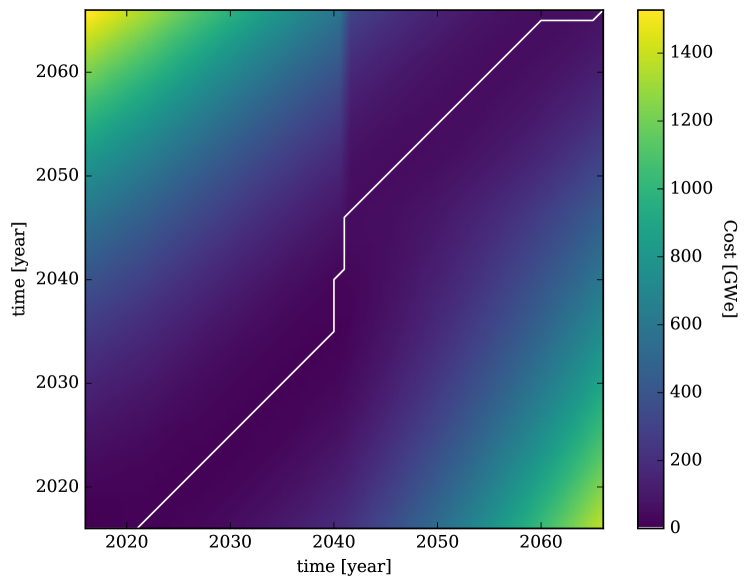
Figure 1: Heat map of the cost matrix between a 1% growth demand curve and a production curve the under produces by 5% for the first 25 years and then over produces for the second 25 years. The warp path $u$ is superimposed as the white curve on top of the cost matrix.

Additionally, the warp path between the example demand and production curves is presented as the white curve on top of the heat map in Figure 1. Recognize that $u$ is monotonic along both time axes. Furthermore, the precise path of $u$ minimizes the cost matrix at every step. Regions of increased cost in the cost matrix can be seen to repel the warp path. The distance $d$ between the demand and production curves here happens to be 0.756 GWe.

Dynamic time warping distance can therefore be used as an objective function to minimize for any demand and production curves. However, using full simulations to find $g(t,\Theta)$ remains expensive, even though DTW itself is computationally cheap. Therefore, a mechanism to reduce the overhead from production curve evaluation is needed.

2.2 Gaussian Process Regression

Evaluating the production curve for a specific kind of facility using full fuel cycle simulations is relatively expensive, even in the computationally cheapest case of low-fidelity simulations. This is because a fuel cycle realization typically computes many features that, though coupled to the production curve, are not directly the production curve. For example, the mass balance of the fuel cycle physically bound the electricity production. However, the mass balances are not explicitly taken into account when trying to meet a power demand curve.

Alternatively, surrogate models that predict the production curve directly have many orders-of-magnitude fewer operations by virtue of not computing implicit physical characteristics. This is not to say that the surrogate models are correct. Rather, they are simply good enough to drive a demand curve optimization. Surrogate models are used here inform a simulator about where in the parameter space to look next. Truth about production curves should still be derived from the fuel cycle simulator and not the surrogate model. In the WORG algorithm, Gaussian processes are used to form the model.

Gaussian processes are more fully covered elsewhere [4]. Using Gaussian process for optimization has also been previously explored [9], though such studies tend not to investigate the integral problems posed by facility deployment. As with dynamic time warping, a minimal but sufficient introduction to GP regression is presented for the purposes of the deployment optimization. Consider the case of $Z$ simulations indexed by $z$ that each have a $\Theta_{z}$ deployment schedule and $g_{z}(t,\Theta_{z})$ production curve.

A Gaussian process of these $Z$ simulations is set by its mean and covariance functions. The mean function is denoted as $\mu(t,\Theta)$ and is the expectation value $\mathbb{E}$ of the series of $G$ inputs:

$$G=\left\{g_{1}(t,\Theta_{1}),g_{2}(t,\Theta_{2}),\ldots,g_{Z}(t,\Theta_{Z})\right\}$$ (8)

The covariance function is denoted $k(t,\Theta,t^{\prime},\Theta^{\prime})$ and is the expected value of the input to the mean. The mean and covariance can be expressed as in Equations 9 & 10 respectively.

$$\mu(t,\Theta)=\mathbb{E}G$$ (9)

$$k(t,\Theta,t^{\prime},\Theta^{\prime})=\mathbb{E}\left[(g_{z}(t,\Theta)-\mu(t,\Theta))(g_{z}(t^{\prime},\Theta^{\prime})-\mu(t^{\prime},\Theta^{\prime}))\right]$$ (10)

Note that in the above, the Gaussian process is itself $P+1$ dimensional, since the means and covariance are a function of both the deployment schedule ($P$) and time ($+1$).

The Gaussian process $\mathpzc{GP}$ approximates the production curve given $Z$ simulations. Allow $*$ to indicate that the a quantity comes from the model as opposed to coming from the results of the simulator. A model production curve can then be written using either functional or operator notation, as appropriate:

$$g_{*}(t,\Theta)\approx\mathpzc{GP}\left(\mu(t,\Theta),k(t,\Theta,t^{\prime},\Theta^{\prime})\right)\equiv\mathpzc{GP}G$$ (11)

In machine learning terminology, $G$ serves as the training set for the GP model.

Now, when performing a regression on Gaussian processes, the nominal functional form for the covariance must be given. Such a functional form is also known as the the kernel function. The kernel contains the hyperparameters that are solved for to obtained a best-fit Gaussian process. The hyperparameters themselves are defined based on the definition of the kernel function. Hyperparameter values are found via a regression of the maximal likelihood of the production curve. Any functional form could potentially serve as a kernel function. However, a generally useful form is the is the exponential squared. This kernel can be seen in Equation 12 with hyperparameters $\ell$ and $\sigma^{2}$ for a vector of parameters $r$:

$$k(r,r^{\prime})=\sigma^{2}\exp\left[-\frac{1}{2\ell}(r-r^{\prime})^{2}\right]$$ (12)

However, other kernels such as the Matérn $3/2$ kernel and Matérn $5/2$ kernel [11] were observed to be more robust for the WORG method. These can be seen in Equations 13 and 14 respectively.

$$k(r,r^{\prime})=\sigma^{2}\left(1+\frac{\sqrt{3}}{\ell}|r-r^{\prime}|\right)\exp\left(-\frac{\sqrt{3}}{\ell}|r-r^{\prime}|\right)$$ (13)

$$k(r,r^{\prime})=\sigma^{2}\left(1+\frac{\sqrt{5}}{\ell}|r-r^{\prime}|+\frac{5}{3\ell^{2}}|r-r^{\prime}|^{2}\right)\exp\left(-\frac{\sqrt{5}}{\ell}|r-r^{\prime}|\right)$$ (14)

From here, say that $\mathbf{K}$ is a covariance matrix such that the element at the $r$-th row and $r^{\prime}$-th column is given by whichever kernel is chosen from Equations 12-14. Then the log likelihood $\log q$ of obtaining the training set production curves $G$ for a given time grid $\mathbf{t}$ and deployment schedule is as seen in Equation 15.

$$\log q(G|\mathbf{t},\Theta)=-\frac{1}{2}G^{\top}\left(\mathbf{K}+\tau^{2}\mathbf{I}\right)^{-1}G-\frac{1}{2}\log\left|\mathbf{K}+\tau^{2}\mathbf{I}\right|-\frac{ZTP}{2}\log 2\pi$$ (15)

Here, $\tau$ is the uncertainty in the production curves coming from the simulations themselves. As most simulators do not report such uncertainties, $\tau$ may be set to floating point precision. $\mathbf{I}$ is the usual identity matrix. The hyperparameters $\ell$ and $\sigma^{2}$ are then adjusted via standard real-valued optimization methods such that Equation 15 is as close to zero as possible. This regression of the Gaussian process itself yields the most likely model of the production curve knowing only a limited number of simulations.

However, the purpose of such a Gaussian process regression is to evaluate the production curve at points in time and for deployment schedules that have not been simulated. Take a time grid $\mathbf{t_{*}}$ and a hypothetical deployment schedule $\Theta_{*}$. Now call the covariance vector between the training set and the model evaluation $\mathbf{k}_{*}=\mathbf{k}(\mathbf{t_{*}},\Theta_{*})$. The production curve predicted by this Gaussian process is then given by the following:

$$\mathbf{g}_{*}(\mathbf{t}_{*},\Theta_{*})=\mathbf{k}_{*}^{\top}\left(\mathbf{K}+\tau^{2}\mathbf{I}\right)^{-1}G$$ (16)

Equations 9-16 are derived and discussed fully in [4].

Implementing the above Gaussian process mathematics for the specific case of the WORG algorithm is not needed. Free and open source Gaussian process modeling software libraries already exist and are applicable to the regression problem here. Scikit-learn v0.17 [12] and George v0.2.1 [13] implement such a method and have a Python interface. George is specialized around Gaussian processes, and thus is preferred for WORG over scikit-learn, which is a general purpose machine learning library.

As an example, consider a Gaussian process between two power production curves similar to the example used in §2.1. The first is a nominal 1% growth in GWe for 50 years starting at 90 GWe in 2016. The second curve under-produces the first curve by 10% for the first 25 years and over-produces by 10% for the last 25 years. Additionally, assume that there is a 10% error on the training set data. This will produce a model of the mean and covariance that splits the difference between these two curves. This example may be seen graphically in Figure 2.

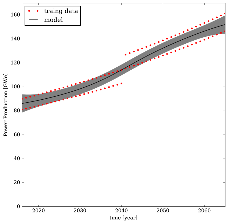
Figure 2: The Gaussian process model of a 1% growth curve along with the an initial 10% under production followed by a 10% under production. The model is represented by the black line that runs between the red training points. Two standard deviations form the model are displayed as the gray region.

The simple example above does not take advantage of an important feature of Gaussian processes. Namely, it is not limited to two production curves in the training set. As many as desirable may be used. This will allow the WORG algorithm to dynamically adjust the number of $Z$ simulations which are used to predict the next deployment schedule. WORG is thus capable of effortlessly expanding $Z$ when new and useful simulations yield valuable production curves. However, it also enables $Z$ to contract to discard production curves that would drive the deployment schedule away from an optimum.

Now that the Gaussian process regression and dynamic time warping tools have been added to the toolbox, the architecture of the WORG algorithm can itself be described.

2.3 WORG Algorithm

The WORG algorithm has two fundamental phases on each iteration: estimation and simulation. These are preceded by an initialization before the optimization loop. Additionally, each iteration decides which information from the previous simulations is worth keeping for the next estimation. Furthermore, the method of estimating deployment schedules may be altered each iteration. Listing 1 shows the WORG algorithm as Python pseudo-code. A detailed walkthrough explanation of this code will now be presented.

Begin by initializing three empty sequences $\vec{\Theta}$, $G$, and $D$. Each element of these series represents deployment schedule $\Theta$, a production curve $g(t,\Theta)$, and a dynamic time warping history between the demand and production curves $d(f,g)$. Importantly, $\vec{\Theta}$, $G$, and $D$ only contain values for the relevant optimization window $Z$. For example, root finding algorithms such as Newton’s method and the bisection method have a length-2 window since they use the $(z-1)^{\mathrm{th}}$ point and the $z^{\mathrm{th}}$ point to compute the $(z+1)^{\mathrm{th}}$ guess. Since a Gaussian process model is formed, any or all of the $s$ iterations may be used. However, restricting the optimization window to be either two or three depending on the circumstances balances the need to keep the points with the lowest $d$ values while pushing the model far from known regions with higher distances. Essentially, WORG tries to have $D$ contain one high-value $d$ and one or two low valued $d$ at all iterations. Such a tactic helps form a meaningfully diverse GP model.

To this end, $\vec{\Theta}$, $G$, and $D$ are initialized with two bounding cases. The first is to set the deployment schedule equal to the lower bound of the number of deployments $M$. Recall that this is usually $\mathbf{0}$ everywhere, unless a minimum number of facilities must be deployed at a specific point in time. Running a simulation with $M$ will then yield a production curve $g(f,g)$ and the DTW distance to this curve. Note that just because the no facilities are deployed, the production curve need not be zero due to the initial conditions of the simulation. Existing initial facilities will continue to be productive.

Similarly, another simulation may be executed for the maximum possible deployment schedule $N$. This will also provide information on the production over time and the distance to the demand curve. $M$ and $N$ form the first two simulations, and therefore the loop variable $s$ is set to two.

Listing 1: WORG Algorithm in Python Pseudo-code

⬇

Thetas, G, D = [], [], [] # initialize history

# run lower bound simulation

g, d = run_sim(M, f)

Thetas.append(M)

G.append(g)

D.append(d)

# run upper bound simulation

g, d = run_sim(N, f)

Thetas.append(N)

G.append(g)

D.append(d)

s = 2

while MAX_D < D[-1] and s < S:

# set estimation method

method = initial_method

if method == 'all' and (s%4 < 2):

method = 'stochastic'

# estimate deployment schedule and run simulation

Theta = estimate(Thetas, G, D, f, method)

g, d = run_sim(Theta, f)

Thetas.append(Theta)

G.append(g)

D.append(d)

# take only the most important and most recent schedules

idx = argsort(D)[:2]

if D[-1] == max(D):

idx.append(-1)

Thetas = [Thetas[i] for i in idx]

G = [G[i] for i in idx]

D = [D[i] for i in idx]

s = (s + 1)

The optimization loop may now be entered. This loop has two conditions. The first is that the next iteration occurs only if the last distance is greater than a threshold value $\mathrm{MAX\_D}$. The second is that the loop variable $s$ must be less than the maximum number of iteration $S$.

The first step in each iteration is to choose the estimation method. The three mechanisms will be discussed in detail in §3. For the purposes of the optimization loop, they may be represented by the ‘stochastic’, ‘inner-prod’, and ‘all’ flags. The stochastic method chooses many random deployment schedules to test. Alternatively, an inner product search of the space defined by $M$ and $N$ may be performed. Lastly, the ‘all’ flag performs both of the previous estimates and takes the one with lowest computed distance. However, ‘all’ can sometimes declare the inner product search the winner for all $s$. This can itself be problematic since this estimation method has the tendency to form deterministic loops when close to an optimum. This behavior is not unlike similar loops formed with floating point approximations to Newton’s method. To prevent this when using ‘all’, WORG forces the stochastic method for two consecutive iterations out of every four.

A best-guess estimate for a deployment schedule $\Theta$ may finally be made. This takes the previous deployment schedules $\vec{\Theta}$ and production curves $G$ and forms a Gaussian process model. Potential values for $\Theta$ are explored according to the selected estimation method. The $\Theta$ that produces the minimum dynamic time warping distance between the demand curve and the model $d(f,g_{*})$ is then returned.

The $\Theta$ estimate is then supplied to the the simulator itself and a simulation is executed. The details of this procedure are, of course, simulator specific. However, the simulation combined with any post-processing needed should return an aggregate production curve $g_{s}(t,\Theta)$. This is then compared to demand curve via $d(f,g_{s})$. After the simulation, $\Theta$, $g_{s}(t,\Theta)$, and $d(f,g_{s})$ are appended to the $\vec{\Theta}$, $G$, and $D$ sequences. Note that the production curve and DTW distance from the simulator are appended, not the production curve and distance from the model estimate.

Concluding the optimization loop, $\vec{\Theta}$, $G$, $D$, and $s$ are updated. This begins by finding and keeping the two elements with the lowest distances between the demand and production curves. However, if the most recent simulation yielded the largest distance, this is also kept for the next iteration. Keeping the largest distance serves to deter exploration in this direction on the next iteration. Thus a sequence of two or three indices is chosen. These indices are applied to redefine $\vec{\Theta}$, $G$, and $D$. Lastly, $s$ is incremented by one and the next iteration begins.

The WORG algorithm presented here shows the overall structure of the optimization. However, equally important and not covered in this section is how the estimation phase chooses $\Theta$. The methods that WORG may use are presented in the following section and completes the methodology.

3 Selecting Deployment Schedule Estimates

There are three methods for choosing a new deployment schedule $\Theta$ to attempt to run in a simulator. The first is stochastic with weighted probabilities for the $\theta_{p}$. The second does a deterministic sweep iteratively over all options, minimizing the dynamic time warping distance at each point in time for each deployment parameter. The last combines these two and choose the one with the minimum distance to the demand curve.

All of these rely on a Gaussian process model of the production curve. This is because constructing and evaluating GP model $g_{*}$ is significantly faster than performing even a low-fidelity simulation. As a demonstrative example, say each evaluation of $d(f,g_{*})$ takes a tenth of a second (which is excessively long) and $d(f,g_{s})$ for a low fidelity simulation takes ten seconds (which is reasonable), the model evaluation is still one hundred times faster. Furthermore, the cost of constructing the GP model can is amortized over the number of guesses that are made.

However, the choice of which $\theta_{p}$ to pick is extremely important as they drive the optimization. In a vanilla stochastic algorithm, each $\theta_{p}$ would be selected as a univariate integer on the range $[M_{p},N_{p}]$. However, this ignores the distance information $D$ that is known about the training set which is used to create the Gaussian process. More intelligent guesses for $\theta_{p}$ focus the model evaluations to more promising regions of the option space. This in turn helps reduce the overall number of expensive simulations needed to find a ‘good enough’ deployment schedule.

The three WORG $\Theta$ selection methods are described in order in the following subsections.

3.1 Stochastic Estimation

The stochastic method works by randomly choosing $\Gamma$ deployment schedules and evaluating $g_{*}(t,\Theta_{\gamma})$ for each guess $\gamma$. The $\Theta_{\gamma}$ which has the minimum distance $d_{\gamma}$ is taken as the best-guess deployment schedule. The number of guesses may be as large or as small as desired. However, a reasonable number to pick spans the option space. This is simply is the $L_{1}$ norm of the difference of the inclusive bounds. Namely, set $\Gamma$ as in Equation 17 for a minimum number of for stochastic guesses.

$$\Gamma=\sum_{p}^{P}(N_{p}-M_{p}+1)$$ (17)

Each $\theta_{p}$ has $N_{p}-M_{p}+1$ options. Thus a reasonable choice for $\Gamma$ is the sum of the number of independent options.

Still, each option for $\theta_{p}$ should not be equally likely. For example, if the demand curve is relatively low, the number of deployed facilities is unlikely to be relatively high. For this reason, the choice of $\theta_{p}$ should be weighted. Furthermore, note that each $\theta_{p}$ is potentially weighted differently as they are all independent parameters. Denote $n\in[M_{p},N_{p}]$ such that the n-th weight for the p-th parameter is called $w_{n,p}$.

To choose weights, first observe that the distances $D$ can be said to be inversely proportional to how likely each deployment schedule in $\vec{\Theta}$ should be. A one-dimensional Gaussian process can thus be constructed to model inverse distances given the values of the deployment parameter for each schedule, namely $\vec{\theta_{p}}$. Call this model $d_{*}^{-1}$ as seen in Equation 18.

$$d_{*}^{-1}(\theta_{p})=\mathpzc{GP}\left(\mu(\vec{\theta_{p}}),k(\vec{\theta_{p}},\vec{\theta_{p}}^{\prime})\right)\equiv\mathpzc{GP}\left[D^{-1}\right]$$ (18)

The construction, regression of hyperparameters, and evaluation of this model follows analogously to the production curve modeling presented in §2.2.

The weights for $\theta_{p}$ are then the normalized evaluation of the inverse distance model for all $m$ and $n$ defined on the p-th range. Symbolically,

$$w_{n,p}=\frac{d_{*}^{-1}(n)}{\sum_{m=M_{p}}^{N_{p}}d_{*}^{-1}(m)}$$ (19)

Equation 19 works very well as long as a valid model can be established. However, this is sometimes not the case when the $\theta_{p}$ are degenerate, the distances are too close together, the distances are too close to zero, or other stability issues arise.

In cases where a valid model may not be formed for $d_{*}^{-1}(\theta_{p})$, a Poisson distribution may be used instead. Take the mean of the Poisson distribution $\lambda$ to be the value of $\theta_{p}$ where the distance is minimized.

$$\lambda_{p}=\theta_{p}|\mathrm{argmin}(D)$$ (20)

Hence, the Poisson probability distribution for the $n$-th weight of the $p$-th deployment parameter is,

$$\mathrm{Poisson(n)}=\frac{(\lambda_{p})^{n}}{n!}e^{-\lambda_{p}}$$ (21)

Now, because $n$ is bounded, it is important to renormalize Equation 21 when constructing stochastic weights.

$$\begin{split}w_{n,p}&=\frac{\frac{(\lambda_{p})^{n}}{n!}e^{-\lambda_{p}}}{\sum_{m=M_{p}}^{N_{p}}\frac{(\lambda_{p})^{m}}{m!}e^{-\lambda_{p}}}\\ &=\frac{(\lambda_{p})^{n}}{n!\sum_{m=M_{p}}^{N_{p}}\frac{(\lambda_{p})^{m}}{m!}}\\ \end{split}$$ (22)

Poisson-based weights could be used exclusively, foregoing the inverse distance Gaussian process models completely. However, a Poisson-only method takes into account less information about the demand-to-production curve distances. It was therefore observed to converge more slowly on an optimum than using Poisson weights as a backup. Since the total number of simulations is aiming to be minimized for in situ use, the WORG method uses Poisson weights as a fallback only.

After weights are computed for all $P$ deployment parameters, a set of $\Gamma$ deployment schedules may be stochastically chosen. The Gaussian process for each $g_{*}(\mathbf{t},\Theta_{\gamma})$ is then evaluated and the dynamic time warping distance to the demand curve is computed. The deployment schedule with the minimum distance is then selected and returned.

3.2 Inner Product Estimation

As an alternative to the stochastic method demonstrated in §3.1, a best-guess for $\Theta$ can also be built up iteratively over all times. The method here uses the same production curve Gaussian process $g_{*}$ to predict production levels and measure the distance to the demand curve. However, this method minimizes the distance at time $t$ and then uses this to inform the minimization of $t+1$. Starting at $t=1$ and moving through the whole time grid to $t=T$, a complete deployment schedule is generated.

The following description is for the simplified case when $P==T$. However, this method is easily extended to the case where $P>T$, such as for multiple reactor types. When $P>T$, group $\theta_{p}$ that occur on the same time step together and take the outer product of their options prior to stepping through time.

For this method, define the time sub-grid $\mathbf{t}_{p}$ as the sequence of all times less than or equal to the time when parameter $p$ occurs, $t(p)$.

$$\mathbf{t}_{p}=\left\{t|t\leq t(p)\right\}$$ (23)

Now define the deployment schedule $\Theta^{t}$ up to time $t$ through the following recursion relations:

$$\begin{split}\theta_{1}&=n\,|\,\mathrm{min}\left[d(f,g_{*}(1,n))\right]\forall n\in[M_{1},N_{1}]\\ \Theta^{1}&=\left\{\theta_{1}\right\}\\ \theta_{p}&=n\,|\,\mathrm{min}\left[d(f,g_{*}(\mathbf{t}_{p},\Theta^{t-1},n))\right]\forall n\in[M_{p},N_{p}]\\ \Theta^{t}&=\left\{\Theta_{1}^{t-1},\ldots,\Theta_{p-1}^{t-1},\theta_{p}\right\}\end{split}$$ (24)

Equation 24 has the effect of choosing the the number of facilities to deploy at each time step that minimizes the distance function. The current time step uses the previous deployment schedule and only searches the option space of the its own deployment parameter $\theta_{p}$. Once $\Theta^{T}$ is reached, it is selected as the deployment schedule $\Theta$. The inner product method here requires the same number of model evaluations of $g_{*}$ as were selected for the default value of $\Gamma$ in Equation 17 for stochastic estimation.

3.3 All of the Above Estimation

This method is simply to run both the stochastic method and the inner product method and determine which has the lower $d(f,g_{*})$ for the deployment schedules they produce. This method contains both the advantages and disadvantages of its constituents. Additionally, it has the disadvantage of being more computationally expensive than the other methods individually.

The advantage from the stochastic method is that the entire space is potentially searched. There are no forbidden regions. This is important since there may be other optima far away from the current $\vec{\Theta}$ that produce lower distances. Searching globally prevents the stochastic method from becoming stuck locally. However, the stochastic method may take many iterations to make minor improvements on a $\Theta$ which is already close to a best-guess. It is, after all, searching globally for something better.

On the other hand, the inner product method is designed to search around the part of the Gaussian process model which already produces good results. It is meant to make minor adjustments as it goes. Unfortunately, this means the inner product method can more easily get stuck in a cycle where it produces the same series of deployment schedules over and over again. It has no mechanism on its own to break out of such cycles.

With the all-of-the-above option, the job of balancing the relative merits of the stochastic and inner product methods is left to the optimization loop itself. This can be seen in §2.3. If the ‘all’ flag is set as the estimation method, it is only executed as the ‘all’ flag two of every four iterations. Other strategies for determining how and when each of the three methods are used could be designed. However, any more complex strategy should be able to show that it meaningfully reduces the number of optimization loop iterations required.

At this point, the entire WORG method has been described. A demonstration of how it performs for a representative fuel cycle is presented in the next section.

4 Results & Performance

To demonstrate the three variant WORG methods, an unconstrained once-through fuel cycle is modeled with the Cyclus simulator [1]. In such a scenario, uranium mining, enrichment, fuel fabrication, and storage all have effectively infinite capacities. The only meaningful constraints on the system are how many light-water reactors (LWR) are built.

The base simulation begins with 100 reactors in 2016 that each produce 1 GWe, have an 18 month batch length with a one month reload time. The initial fleet of LWRs retires evenly over the 40 years from 2016 to 2056. All new reactors have 60 year life times. The simulation itself follows 20 years from 2016 to 2035. This is on the higher end of in situ time horizons expected, which presumably will be in the neighborhood of 1, 5, 10, or 20 years.

The study here compares how WORG performs for 0% (steady state), 1%, and 2% growth curves from an initial 90 GWe target. These are examined using the three estimation methods variants described in the previous section. Calling $\rho$ the growth rate as a fraction, the demand curve is thus,

$$f(t)=90(1+\rho)^{t}$$ (25)

Moreover, the upper bound for the number of deployable facilities at each time is set to be the ceiling of ten times the total growth. That is, assuming ten facilities at most could be deployed in the first year, increase the upper bound along with the growth rate. This yields the following expression for $N$.

$$N(t)=\left\lceil 10(1+\rho)^{t}\right\rceil$$ (26)

The lower bound for the number of deployed reactors is taken to be the zero vector, $M=\mathbf{0}$. A maximum of twenty simulations are allowed, or $S=20$. This is because an in situ method cannot afford many optimization iterations. The random seed for all optimizations was 424242.

Note that because of the integral nature of facility deployment, exactly matching a continuous demand curve is not possible in general. Slight over- and under-prediction are expected for most points in time. Furthermore, it is unlikely that the initial facilities will match the demand curve themselves. If the initial facilities do no meet the demand on their own, then the optimized deployment schedule is capable making up the difference. However if the initial facilities produce more than the demand curve, the the optimizer is only capable of deploying zero facilities at these times. The WORG method does not help make radical adjustments to accommodate problems with the initial conditions, such as when 50 GWe are demanded but 100 GWe are already being produced.

First examine Figures 3 - 5 which show the optimized deployment schedule for the three estimation methods. The figures represent the 0%, 1% and 2% growth curves respectively. Figures 3 & 4 show that the ‘stochastic’ method has the highest number of facilities deployed at any single time. In the 2% case, the ‘all’ method predicts the largest number of facilities deployed.

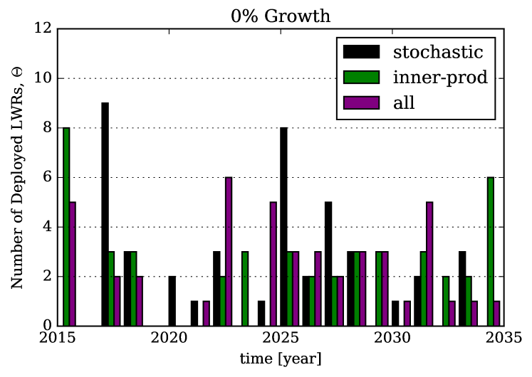
Figure 3: Optimized deployment schedule $\Theta$ for a 0% growth (steady state) demand curve. The number of deployed facilities shown are for the ‘stochastic’ (black), ‘inner-prod’ (green), and ‘all’ (purple) estimation methods.

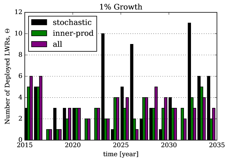
Figure 4: Optimized deployment schedule $\Theta$ for a 1% growth demand curve. The number of deployed facilities shown are for the ‘stochastic’ (black), ‘inner-prod’ (green), and ‘all’ (purple) estimation methods.

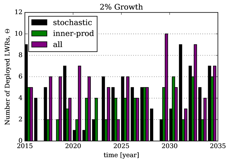
Figure 5: Optimized deployment schedule $\Theta$ for a 2% growth demand curve. The number of deployed facilities shown are for the ‘stochastic’ (black), ‘inner-prod’ (green), and ‘all’ (purple) estimation methods.

More important than the deployment schedules themselves, however, are the production curves that they elicit. Figures 6 - 8 display the power production for the best-guess deployment schedule $G_{1}$ (solid lines), production for the second best schedule $G_{2}$ (dotted lines), and demand curves (dashed lines) for 0%, 1%, and 2% growth. The figures show each estimation mechanism separately.

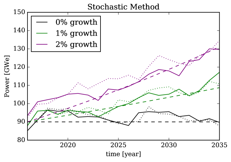
Figure 6: Power production to demand comparison for 20 year deployment schedule optimization using only the ‘stochastic’ estimation method. 0%, 1%, and 2% growth rates starting at 90 GWe are shown. Solid lines represent the best guess deployment schedule. Dotted lines are represent the second best guess deployment schedule. Dashed lines represent the demand curve that is targeted.

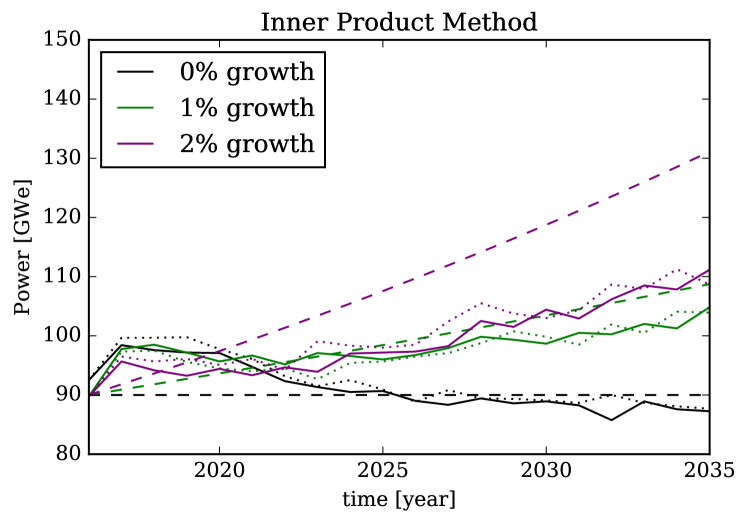
Figure 7: Power production to demand comparison for 20 year deployment schedule optimization using only the ‘inner-prod’ estimation method. 0%, 1%, and 2% growth rates starting at 90 GWe are shown. Solid lines represent the best guess deployment schedule. Dotted lines are represent the second best guess deployment schedule. Dashed lines represent the demand curve that is targeted.

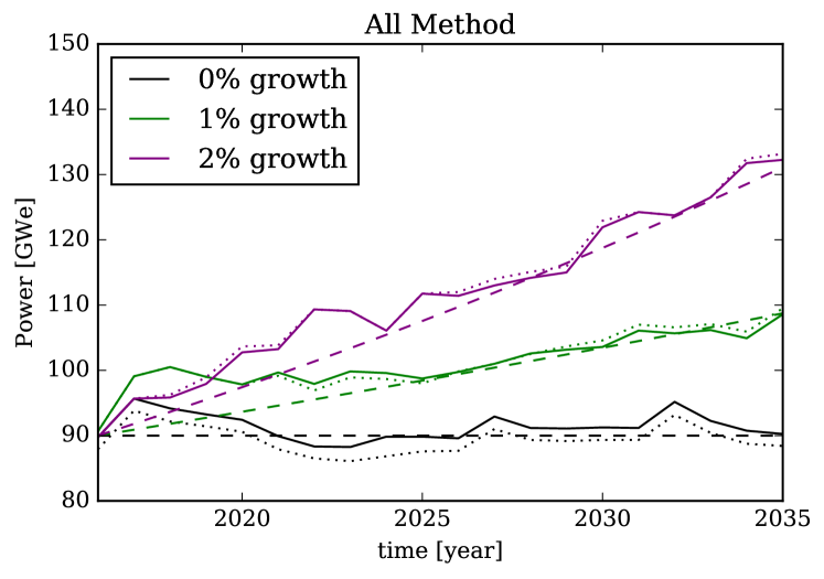
Figure 8: Power production to demand comparison for 20 year deployment schedule optimization using the ‘all’ estimation method that selects the best of both ‘stochastic’ and ‘inner-prod’ estimations. 0%, 1%, and 2% growth rates starting at 90 GWe are shown. Solid lines represent the best guess deployment schedule. Dotted lines are represent the second best guess deployment schedule. Dashed lines represent the demand curve that is targeted.

As seen in Figure 6, the ‘stochastic’ only estimations follow the trend line of the growth curve. However, only for a few regions such as for 2% growth between 2025 - 2030, does the production very closely match the the demand. The second best guess for the deployment schedule shows a relatively large degree of eccentricity. This indicates that $G_{2}$ at the end of the optimization is there to show the Gaussian process model regions in the $\Theta$ option space that do not work.

Alternatively the inner product search estimation can be seen in Figure 7. This method does a reasonable job of predicting a steady state scenario at later times. However, the 1% and 2% curves are largely under-predicted. For the 2% case, this is so severe as to be considered wholly wrong. This situation arises because the ‘inner-prod’ method can enter into deterministic traps where the same cycle of deployment schedules is predicted forever. If such a trap is fallen into when the production curve is far from an optimum, the inner product method does not yield a sufficiently close guess of the deployment schedule.

However, combining the stochastic and inner product estimation methods limits the weakness of each method. Figure 8 shows the production and demand information for the ‘all’ estimation flag. By inspection, this method produces production curves that match the demand much more closely. This is especially true for later times. Over-prediction discrepancies for early times come from the fact the initially deployed facilities (100 LWRs with 18 month cycles) does not precisely match an initial 90 GWe target. The problem was specified this way in order to show that reasonable deployments are still selected even in slightly unreasonable situations.

Still, the main purpose of the WORG algorithm is to converge as quickly as possible to a reasonable best-guess $\Theta$. The limiting factor is the number of predictive simulations which must be run. WORG will always execute at least three full simulations: the lower bound, the upper bound, and one iteration of the optimization loop. A reasonable limit on the total number of simulations $S$ is 20. For an in situ calculator, it is unlikely to want to compute more than this number of sub-simulations to predict the deployment schedule for the next 1, 5, 10, or 20 years. However, it may be possible to limit $S$ to significantly below 20 as well.

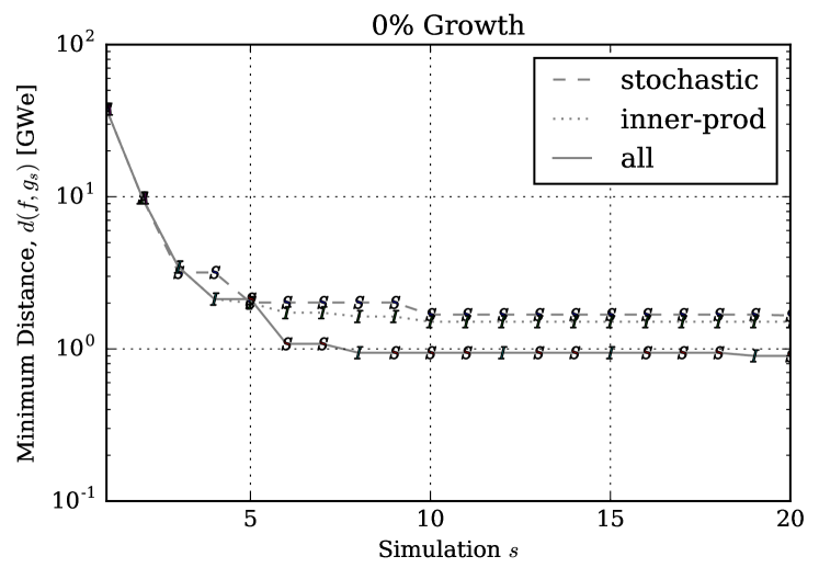
Figure 9: Convergence of 0% growth rate solution for the distance between the demand and production curves $d(f,g)$ as a function of the number of simulations. The three estimation methods are shown. Additionally, the $S$, $I$, and $A$ marker represent whether the ‘stochastic’, ‘inner-prod’, or ‘all’ method was selected as the best fit. For $2<s$, the ‘all’ will select either $S$ or $I$.

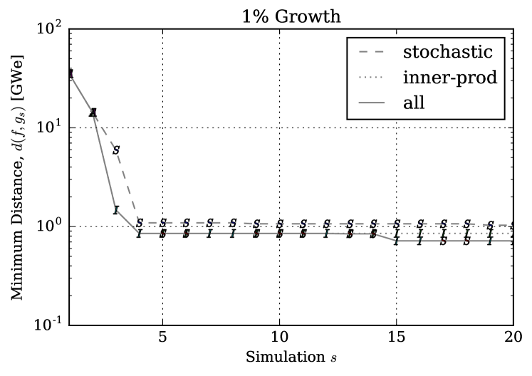
Figure 10: Convergence of 1% growth rate solution for the distance between the demand and production curves $d(f,g)$ as a function of the number of simulations. The three estimation methods are shown. Additionally, the $S$, $I$, and $A$ marker represent whether the ‘stochastic’, ‘inner-prod’, or ‘all’ method was selected as the best fit. For $2<s$, the ‘all’ will select either $S$ or $I$.

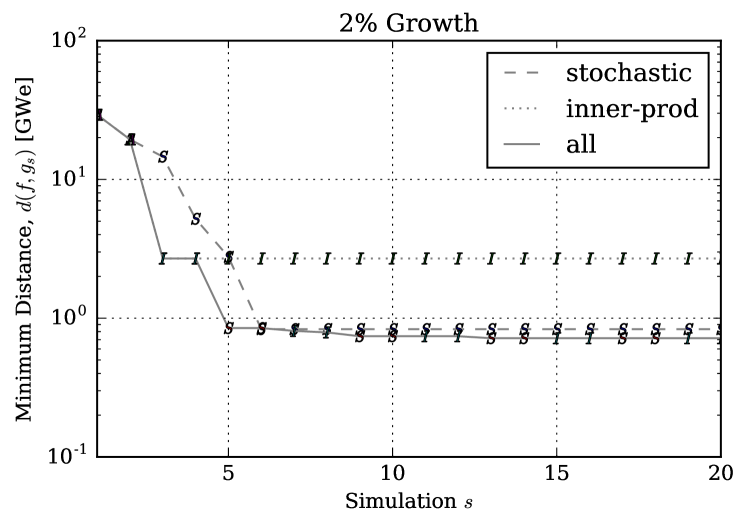
Figure 11: Convergence of 2% growth rate solution for the distance between the demand and production curves $d(f,g)$ as a function of the number of simulations. The three estimation methods are shown. Additionally, the $S$, $I$, and $A$ marker represent whether the ‘stochastic’, ‘inner-prod’, or ‘all’ method was selected as the best fit. For $2<s$, the ‘all’ will select either $S$ or $I$.

Figures 9 - 11 demonstrate a convergence study for the three different growth rates as a function of the number of simulations $s$. These three figures demonstrate important properties of the WORG method. The first is that the ‘all’ estimation method here consistently has the lowest minimum dynamic time warping distance, and thus the best guess for the deployment schedule $\Theta$. Furthermore, the ‘all’ curves in these figures show that the best estimation method consistently switches between the inner product search and stochastic search. These imply that together the ‘stochastic’ and ‘inner-prod’ methods converge more quickly that the sum of their parts. This is particularly visible in the 0% growth rate case seen in Figure 9.

Additionally, These convergence plots show that the majority of the $\Theta$ selection gains are made by $s=10$. Simulations past ten may show differential improvement for the ‘all’ method. However, they do not tend to generate any measurable improvement for ‘stochastic’ or ‘inner-prod’ selection mechanisms. Furthermore, most of the gains for the ‘all’ method are realized by simulation five or six. Thus a reduction by a factor of two to four in the number of simulations is available. This equates directly to a like reduction in computational cost.

Moreover, Figures 9 - 11 also show the tendency of the ‘inner-prod’ method to become deterministically stuck when used on its own. In all three cases the ‘inner-prod’ method resolves to a constant by simulation five or ten. In the 1% case, this solution happens to be quite close to the solution predicted by the ‘all’ method. In the 0% case, this constant is meaningfully distinct, but is still more akin to the ‘stochastic’ solution than the ‘all’ solution. In the 2% case, the converged ‘inner-prod’ result has little to do with the ‘all’ prediction. Thus it is not recommended to use ‘inner-prod’ on its own. While it may succeed, it is too risky because it may cease improving at the wrong place.

The ‘stochastic’ estimation method is also prone to similar cyclic behavior. However, in the ‘inner-prod’ method, is the second best guess $G_{2}$ is also in a constant prediction cycle along with $G_{1}$. With the stochastic search, the second best guess has more freedom to roam the option space, creating potentially different Gaussian process models with each iteration $s$. Eventually, given enough guesses and enough iterations, the stochastic model will break out of a local optimum to perhaps find a better global optimum elsewhere. For the in situ use case, though, eventual solution is not fast enough. The inner product search spans regions that the stochastic weighting labeled as unlikely. This assist is what enables the ‘all’ method to converge faster than the stochastic method on its own. That said, if the in situ use case is not relevant, the stochastic method on its own could be used without any algorithmic qualms.

5 Conclusions & Future Work

The WORG method provides a deployment schedule optimizer that converges both closely enough and fast enough to be used inside of a nuclear fuel cycle simulator. The algorithm can consistently obtain tolerances of half-a-percent to a percent (1 GWe distances for over 200 GWe deployable) for the once-through fuel cycle featured here within only five to ten simulations. Such optimization problems are made more challenging due to the integral nature of facility deployment and that any demand curve may be requested.

WORG works by setting up a Gaussian process to model the production as a function of time and the deployment schedule. This model may then be evaluated orders of magnitude faster than running a full simulation, enabling the search over many potential deployment schedules. The quality of these possible schedules is evaluated based on the dynamic time warping distance to the demand curve. The lowest distance curve is then evaluated in a full fuel cycle simulation. The production curve that is computed by the simulator in turn goes on to update the Gaussian process model and the cycle repeats until the limiting conditions are met.

However, choosing the deployment schedules to estimate with the Gaussian process may be performed in a number of ways. A blind approach would simply be to choose such schedules randomly from a univariate. However, the WORG method has more information available to it that helps drive down the number of loop iterations. The first method discussed remains stochastic but uses the inverse DTW distances of the GP model to weight the deployment options, falling back to a Poisson distribution as necessary. This second method minimizes the model distance for each point in time from start to end, iteratively building up a solution. Finally, another estimation strategy tries both previous options and chooses the best result, forcing the stochastic method two of every four iterations to avoid deterministic loops. It is this last all-of-the-above method that is seen to converge the fastest and to the lowest distance in most cases.

It is important to note that the WORG algorithm is applicable to any demand curve type and fuel cycle facility type. It is not restricted to reactors and power. Enrichment and separative work units, reprocessing and separations capacity, and deep geologic repositories and their space could be deployed via the WORG method for any applicable demand curve. Reactors were chosen for study here as the representative keystone example.

The next major step for this work is to actually employ the WORG method in a fuel cycle simulator. However, to the best knowledge of the author, no existing simulator is capable of spawning forks of itself during run time, rejoining the processes, and evaluating the results of the child simulations in the parent simulation. Concisely, while many simulators are ‘dynamic’ in the fuel cycle sense, none are ‘dynamic’ in the programming language sense. This latter usage of the term is what is required to take advantage of any sophisticated in situ deployment optimizer. The Cyclus fuel cycle simulator looks most promising as a platform for such work to be undertaken. However, many technical roadblocks on the software side remain, even for Cyclus.

Furthermore, adding in situ capability also adds the additional degree of freedom of how often to run the deployment schedule optimizer. Running WORG each and every time step seems excessive a priori. Is every year, five years, or ten years sufficient? How does this degree of freedom balance with the time horizon $T$ specificed in the optimizer? These questions remain unanswered, even in a heuristic sense, and thus the frequency of optimization will be a key parameter in a future in situ study.

References

- [1] K. D. HUFF et al., “Fundamental Concepts in the Cyclus Fuel Cycle Simulator Framework,” CoRR, abs/1509.03604 (2015).
- [2] R. W. CARLSEN et al., “Cyclus v1.0.0,” (2014), http://dx.doi.org/10.6084/m9.figshare.1041745.
- [3] M. MÜLLER, “Dynamic Time Warping,” in Information Retrieval for Music and Motion, pages 69–84, Springer Berlin Heidelberg, 2007.
- [4] C. E. RASMUSSEN and C. K. WILLIAMS, Gaussian processes for machine learning, The MIT Press (2006).
- [5] W. D. KELTON and A. M. LAW, Simulation modeling and analysis, McGraw Hill Boston (2000).
- [6] R. J. VANDERBEI, “Linear programming,” Foundations and Extensions. Second Edition-International Series in Operations Research and Management Science, 37 (2001).
- [7] J. KENNEDY, “Particle swarm optimization,” in Encyclopedia of Machine Learning, pages 760–766, Springer, 2010.
- [8] A. I. F. VAZ and L. N. VICENTE, “PSwarm: A hybrid solver for linearly constrained global derivative-free optimization,” Optimization Methods & Software, 24, 669 (2009).
- [9] M. A. OSBORNE, R. GARNETT, and S. J. ROBERTS, “Gaussian processes for global optimization,” Proc. 3rd international conference on learning and intelligent optimization (LION3), pages 1–15, 2009.
- [10] T. W. SIMPSON, T. M. MAUERY, J. J. KORTE, and F. MISTREE, “Kriging models for global approximation in simulation-based multidisciplinary design optimization,” AIAA journal, 39, 2233 (2001).
- [11] C. PACIOREK and M. SCHERVISH, “Nonstationary covariance functions for Gaussian process regression,” Advances in neural information processing systems, 16, 273 (2004).
- [12] F. PEDREGOSA et al., “Scikit-learn: Machine Learning in Python,” Journal of Machine Learning Research, 12, 2825 (2011).
- [13] S. Ambikasaran, D. Foreman-Mackey, L. Greengard, D. W. Hogg, and M. O’Neil, “Fast Direct Methods for Gaussian Processes and the Analysis of NASA Kepler Mission Data,” (2014).