1 INTRODUCTION

This work uses the meta-analysis method (the analysis of analyses). This method extensively was used already in $18-19$th centuries by Laplace [1] and astronomers [2] though this idea has been appeared even earlier among astronomers in $17$th century and was developing further, especially after invention by Blaise Pascal the mathematical ways of dealing with the games of chance used for gambling. The main goal of this work is to figure out the possible phase diagram of strongly interacting matter using already available published material obtained during decades.

The work is organized as follows. In the next section, a simple form of the mathematical foundation of the meta-analysis is shown. Section 3 is devoted to the application of the obtained formulas to the published results from experimental and theoretical investigations in the ultra-relativistic central nucleus-nucleus collisions. Section 4 contains conclusion.

2 JUSTIFICATION OF THE METHOD

Let’s consider some phenomenon $P$ of arbitrary nature. Let this phenomenon consist of several subprocesses: $P=\{p_{1},p_{2},...,p_{y}\}$. Let this phenomenon exist during a time interval and within some spatial volume $a_{P}=\{\tau_{f}(P)\,-\,\tau_{0}(P);V_{f}(P)\}$, and each subprocess also occupies own space-time interval: $a_{p_{i}}=\{\tau_{f}(p_{i})\,-\,\tau_{0}(p_{i});V_{f}(p_{i})\}$, such that $a_{p_{i}}\in{a_{P}},\,\forall{i}$. Let we observe a phenomenon $P$ through measurements of some set of observables $S(B)=\{B_{1},...,B_{x}\}$. Each $B_{i}$ is responsible for several subprocesses which influence on $B_{i}$: $s(B_{i})=\{p_{m},..,p_{r}\}\subset{P}$. Or, what the same, each subprocess $p_{i}$ gives a contribution to several observables $s(p_{i})=\{B_{j},...,B_{t}\}\subset{S(B)}$.

Let experiment can measure any observable $B_{i}\in{S(B)}$ within some interval of its change defined by an experimental conditions and this interval is broken into $n_{B_{i}}$ small bins (number of data points) with width determined by the sensitivity of experiment to $B_{i}$ and by the problem definition. A set of measured points of $B_{i}$ is $B^{exp}_{i}=\{B^{exp}_{i,1}\pm\sigma^{exp}(B_{i,1}),...,B^{exp}_{i,n_{B_{i}}}\pm\sigma^{exp}(B_{i,n_{B_{i}}})\}$, where $\sigma^{exp}(B_{i,j})$ is an experimental error corresponded to the $j$th point of data. For each subprocess $p_{i}\in{P}$, there is a set of measured observables on which $p_{i}$ influence: $s^{exp}(p_{i})=\{B^{exp}_{j},...,B^{exp}_{t}\}\subset{s(p_{i})}\subset{S(B)}$.

Now let’s consider a set of the theories $S(T)=\{T_{1},...,T_{s}\}$ describing the considered phenomenon $P$. Each model $T_{i}$ describes a phenomenon $P$, considering its consisting of a set of the subprocesses $P(T_{i})=\{t_{1}(T_{i}),...,t_{w}(T_{i})\}$ defined within phenomenology of the theory $T_{i}$. Note that the number of elements of sets $P$ and $P(T_{i})$ can be different. Let the theory $T_{i}$ allows to calculate all set of the observables $S(B)$, giving a set $S_{T_{i}}(B)=\{B_{1}(T_{i}),...,B_{x}(T_{i})\}$. Each $B_{j}(T_{i})$ is responsible for several subprocesses which influence on $B_{j}(T_{i})$: $s(B_{j}(T_{i}))=\{t_{q}(T_{i}),..,t_{v}(T_{i})\}\subset{P(T_{i})}$. Or, what the same, each subprocess $t_{r}(T_{i})$ gives a contribution to the set of observables $s(t_{r}(T_{i}))=\{B_{d}(T_{i}),...,B_{g}(T_{i})\}\subset{S_{T_{i}}(B)}$. For each $B^{exp}_{j}$, theoretical value should be calculated $B^{th}_{j}(T_{i})=\{B^{th}_{j,1}(T_{i})\pm\sigma^{th}(B_{j,1}(T_{i})),...,B^{th}_{j,n_{B_{j}}}(T_{i})\pm\sigma^{th}(B_{j,n_{B_{j}}}(T_{i}))\}$, where $\sigma^{th}(B_{j,f}(T_{i}))$ is an theoretical error corresponded to the $f$th point of data. Identity of theoretical subprocess $t_{r}(T_{i})$ to real $p_{k}$ can be checked by the comparison of the theoretical set $s(t_{r}(T_{i}))$ and set of measured observables $s^{exp}(p_{k})$. Having executed this comparison for all subprocesses from $P(T_{i})$ (or for all observables) it is possible to estimate adequacy of the theory $T_{i}$ in the description of a phenomenon $P$. Let’s introduce for this purpose a set of criteria $s_{T_{i}}(f(B_{j}))=\{f_{1,T_{i}}(B_{j}),...,f_{z,T_{i}}(B_{j})\}$. Each $f_{u,T_{i}}(B_{j})$ is a some function of theoretically calculated and measured observable $B_{j}$, their experimental and theoretical errors $\sigma^{exp(th)}(B_{j})$:

$$f_{u,T_{i}}(B_{j})=\sum f_{u}(B^{th}_{j}(T_{i}),B^{exp}_{j})\pm\sigma(f_{u,T_{i}}),$$ (1)

where summation runs over all data points of $B_{j}$ and:

$$\sigma(f_{u,T_{i}})=\sqrt{\sum(\frac{\partial{f_{u}}}{\partial{B^{th}_{j}}}\sigma^{th})^{2}+\sum(\frac{\partial{f_{u}}}{\partial{B^{exp}_{j}}}\sigma^{exp})^{2}},\mbox{ if }\sigma^{th,exp}\ll B^{th,exp},$$ (2)

otherwise

$$\sigma(f_{u,T_{i}})=\sum c_{1}\cdot\sigma^{th}(B_{j}(T_{i}))+\sum c_{2}\cdot\sigma^{exp}(B^{exp}_{j}),$$ (3)

where $c_{1(2)}$ depends from a type of functional dependence of $B^{exp(th)}_{j}$ in $f_{u,T_{i}}(B_{j})$. Having done these calculations according to (1 - 3) for all measured observables, we will receive a set of sets of various types of criteria: $s_{T_{i}}(f(B))=\{s_{T_{i}}(f(B_{1})),...,s_{T_{i}}(f(B_{x}))\}$. To obtain an information about adequacy of the description by the theory $T_{i}$ of phenomenon $P$, we will carry out summation of criteria of one type over all measured observables:

$$f_{u,T_{i}}(B)=\sum\limits_{j=1}^{x}f_{u,T_{i}}(B_{j}),u\in{[1,z]}.$$ (4)

Having repeated calculations according to (1 - 4) for all theories of $S(T)$, we will be able to choose the best theory with the set of criteria $s_{T_{i}}(f(B))$ containing the greatest number of the smallest criteria of any type (this is meaning that the best agreement of the theory with experiment gives the smallest criterion, irrespectively to the criterion’s type).

If theories use results of measurements of the different experiments, which obtained different number of data points for the same observable and different limits of its measurement defined by the experimental conditions, then comparison of the criteria calculated according to (1 - 4) for different theories will be incorrect. In addition, let theories were applied to the different number of observables, measured in the different experiments. Let the minimum and maximum value of measured observable $B_{j}$ in the $l$th experiment is $B^{exp.l}_{j;\,min}$ and $B^{exp.l}_{j;\,max}$ respectively. Then experimentally covered area of measurements in the $l$th experiment is: $\Omega_{l}\,=\,\bigcup\limits_{j=1}^{c}[B^{exp.l}_{j;\,min},B^{exp.l}_{j;\,max}],$ where number of measured observables $c$ is a different for each $l$. If we average the expression (1) over number of data points $n_{B_{j}}$:

$$\Phi_{u,T_{i}}(B_{j})=\frac{1}{n_{B_{j}}}\cdot(f_{u,T_{i}}(B_{j})\pm\sigma(f_{u,T_{i}})),$$ (5)

and average the expression (5) over number of measured observables $c$:

$$\Phi_{u,T_{i}}(B)=\frac{1}{c}\cdot\sum\limits_{j=1}^{c}\Phi_{u,T_{i}}(B_{j}),$$ (6)

we have received the criterion of $u$th type for theory $T_{i}$ which is equally spread over measurement’s area $\Omega_{l}$ of $l$th experiment. Having done this averaging for all set of theories $S(T)$, we can correctly compare criteria of different theories $\Phi_{u,T_{i}}(B)$ having minimized influence on the criteria of an inequality of the numbers of measured observables used by different theories and an inequality of areas of measurements $\Omega_{l}$ of different experiments.

If it is impossible to tell precisely which theory is better describes an experiment and, therefore, it is impossible to understand a phenomenon $P$, it makes sense to combine (to average) criteria of theories describing $P$ in the similar way - they assume existence of some subprocess $p_{i}$ identifying with it own subprocess $t_{o}(T_{j})$, where $j$ runs over all such theories. To compare combined criterion of these theories $\Phi_{u,T}(B),\,(T\,=\,T_{\alpha}\otimes...\otimes T_{\kappa}$, $\otimes$ is meaning a averaging of criteria of theories from left and right side from simbol), with the combined criterion of theories $\Phi_{u,\bar{T}}(B),\,(\bar{T}\,=\,T_{\lambda}\otimes...\otimes T_{\omega})$, are not considering this subprocess $p_{i}$ inside phenomenon $P$, we should check that all other subprocesses which included inside the theories from $T$ (or $\bar{T}$) should not contradict to each other (the rule of a combination of theories), otherwise criterion $\Phi_{u,T_{\alpha}\otimes...\otimes T_{\kappa}}(B)$ (or $\Phi_{u,T_{\lambda}\otimes...\otimes T_{\omega}}(B)$) has not sense because theory $T_{\alpha}\otimes...\otimes T_{\kappa}$ (or $T_{\lambda}\otimes...\otimes T_{\omega}$) contains mutually incompatible subprocesses. In the previous work [3] this rule was violated, therefore conclusions were made by me and co-authors the absolutely wrong. The combination of theories is understood further as averaging of their criteria.

In the reasonings stated above, the measured observable $B^{exp}_{i}$ is understood as the quantity which can be directly measured in the experiment. For functions with algebraic actions applied upon the measured observables, formulas (1 - 6) have to be changed. Let’s consider a function of any number of the measured observables with an arbitrary dependence between them: $\Gamma\,=\,\Gamma(B^{exp}_{1},...,B^{exp}_{\rho})$. Let some theory $T_{j}$ allows to calculate the same function: $\Gamma(T_{j})\,=\,\Gamma(B^{th}_{1}(T_{j}),...,B^{th}_{\rho}(T_{j}))$. It is obvious, that the criterion of comparison $F$ of theoretically calculated function $\Gamma(T_{j})$ and received from the measured observables $\Gamma$ is obliged to consider not only values of these two functions, but also all criteria of comparison of the theoretically calculated observables $B^{th}_{i}(T_{j}),\,i\in[1,\rho]$, with the measured observables $B^{exp}_{i},\,i\in[1,\rho]$: $F_{u,T_{j}}(\Gamma)=F(\Phi_{u,T_{j}}(\Gamma),\Phi_{u,T_{j}}(B_{1}),...,\Phi_{u,T_{j}}(B_{\rho})),$ where $\Phi_{u,T_{j}}(\Gamma)$ is calculated according to (5) (without summation and averaging here) with replacement $B_{j}\rightarrow\Gamma$, and $\Phi_{u,T_{j}}(B_{i})$ - exactly according to (5). The simplest form of $F_{u,T_{j}}(\Gamma)$ then can be written as:

$$F_{u,T_{j}}(\Gamma)=\frac{1}{2}\cdot(\Phi_{u,T_{j}}(\Gamma)+\Phi_{u,T_{j}}(B)),$$ (7)

where first summand inside bracket consider the structure of $\Gamma$, and second summand calculated according to (6) consider agreement theory with all measured observables. Thus, the calculated criterion $F$ excludes accidental agreement theory with combined function of several observables if calculation of second summand inside bracket of (7) is not made.

Let some subprocess $p_{\varepsilon}\in{P}$ happens in a negligible space-time interval $a_{p_{\varepsilon}}=\{\tau_{f}(p_{\varepsilon})\,-\,\tau_{0}(p_{\varepsilon});V_{f}(p_{\varepsilon})\},$ which is a tiny in the comparison with space-time interval of the phenomenon $P$ and all other subprocesses from $P$: $a_{p_{\varepsilon}}\,\ll\,a_{P},\,a_{p_{\varepsilon}}\,\ll\,a_{p_{i}},\,\forall{i\neq{\varepsilon}}$. Let this subprocess gives a contribution into the measured observables from set $s^{exp}(p_{\varepsilon})=\{B^{exp}_{\beta},...,B^{exp}_{\mu}\}\subset{S(B)}$. Each $B^{exp}_{i}\in{s^{exp}(p_{\varepsilon})}$ is influenced by several subprocesses from set $s(B^{exp}_{i})=\{p_{m},..,p_{r}\}\subset{P}$. At first sight, it will be impossible to distinguish subprocess $p_{\varepsilon}$ since it is suppressed by a contribution from other subprocesses. Now we should take into account that for experimental observable $B^{exp}_{i}\in{s^{exp}(p_{\varepsilon})}$ there is a set of measurements corresponded to $n_{B_{i}}$ data points: $B^{exp}_{i}=\{B^{exp}_{i,1}\pm\sigma^{exp}(B_{i,1}),...,B^{exp}_{i,n_{B_{i}}}\pm\sigma^{exp}(B_{i,n_{B_{i}}})\}$. Let’s introduce a hypothesis $H$.

${\bf H:\,}$Among all observables from $s^{exp}(p_{\varepsilon})\subset{S(B)}$ there is at least one, $B^{exp}_{i},\,i\in{[\beta,\mu]}$, which has at least one such $g$th point of data, $B^{exp}_{i,g}\pm\sigma^{exp}(B_{i,g})$, which is influenced by subprocess $p_{\varepsilon}$ in the not small degree at least comparable to the influences from other subprocesses. I.e., in a very narrow area of measurements corresponded to this $g$th point of data, subprocess $p_{\varepsilon}$ gives a largest contribution in the comparison to its influences in the other data points.

Let there is a set of theories $T(\bar{p}_{\varepsilon})\in{S(T)}$ each of which does not assumes existence of the subprocess $p_{\varepsilon}$ in the phenomenon $P$. According to hypothesis $H$ each of these theories should have the maximal difference between theoretically calculated and measured observable in $g$th point of data of $B^{exp}_{i}$ in comparison with differences in other data points. If, in the analysis, we use only one point of data of each observable, where difference between theory and measurements is largest, we artificially separate the area with, probably, the largest manifestation of the $p_{\varepsilon}$. Having calculated and averaged criteria calculated for such points over all observables and having combined all theories according to the rule of a combination, the obtained criteria $\Phi_{u,T_{1}(\bar{p}_{\varepsilon})\otimes...\otimes T_{e}(\bar{p}_{\varepsilon})}(B),\,T_{i}\in{T(\bar{p}_{\varepsilon})},i\in{[1,e]}$, should be maximal if $p_{\varepsilon}$ appears in $P$. Let’s call such criteria corresponded only to one point of data with largest difference between theory and experiment - the worst criteria.

Otherwise, for a set of mutually compatible theories $T(p_{\varepsilon})\in{S(T)}$ each of which assumes existence of subprocess $p_{\varepsilon}$ in the phenomenon $P$ the worst criterion $\Phi_{u,T_{1}(p_{\varepsilon})\otimes...\otimes T_{n}(p_{\varepsilon})}(B),\,T_{i}\in{T(p_{\varepsilon})},i\in{[1,n]}$, should be less than $\Phi_{u,T_{1}(\bar{p}_{\varepsilon})\otimes...\otimes T_{e}(\bar{p}_{\varepsilon})}(B)$.

One more reason of using only worst criteria calculated only for one point of data for each observable is next. Each developer of any theory wants to describe experimental data within experimental errors. If theory describes the most part of experimental data points for some observable within experimental errors, then calculation of criterion with averaging over all data points (5) will shade a divergence in a points with the worst agreement of theory with measurements. But we need an objective assessment of the theory, and the phenomenon can be understood and studied completely if the theory does not give any divergence with measurements anywhere inside the area of measurements $\Omega_{j},\,\forall j$, where $j$ is a name of experiment. Having kept for the analysis only a area of measurements with the worst agreement of the theory with experiment $\Omega^{worst}_{j}\subset{\Omega_{j}}$ we, thereby, isolated a problem area and further we work only within this problem, coming closer as it is possible to a noumenon of the studied phenomenon. That is, if the phenomenon so difficult that for its full understanding necessaryly creation of difficult mathematical model and construct the new expensive devices, i.e. necessary the big expenses of time and resources, then one of the possible ways to learn the phenomenon is to carry out the analysis of area of the worst agreement of the theory with experiment where a number of subprocesses are not considered by theory because of their complexity for the mathematical description and experimental measurement.

In the [1] and [2], the meta-analysis was applyed to the experimental data. If theory is a reflection of the nature expressed in the mathematical form, then meta-analysis should be also applicable to the theory which should take into account an initial and boundary conditions of combined experiments and conservation laws which, of couse, always work in the experiment. Otherwise the predictions of theory and experimental data of combined measurements never can be compared. In the above shown method, the meta-analysis was applyed to the criteria, i.e. to the functions of values applicable for the meta-analysis. Therefore, the criteria also applicable to the meta-analysis.

The meta-analysis in the form described above uses all available theoretical data applyed to experimental data without any restriction on observables, in contrast with the often used fitting of experimental data by trimming a set of parameters of the used theory. In the last case, the used observables are restricted crucially and final analysis is carryed out only in the area of the best fitting, does not paying attantion to the large heap of the not used observables and sometimes, if fitting was applyed to the function of observables, even without interest how their theory with the best parameters of fitting describes separately the observables included in the fitted function. Moreover, the used parameters of fitting are attributed to the phenomenon under investigation as physical values characterising phenomenon but which can be absent in real phenomenon. The meta-analysis uses the completed form of theory without any trimmings. The analysis of area of the worst agreement of theory with experiment can gives possibility to clarify the structure of phenomenon even if the used theories do not contain lot of subprocesses from phenomenon, by using phenomenology still not enveloped in the mathematical form applicable for the comparison with experimental data.

3 APPLICATION OF THE METHOD

In this work, I use the set of worst criteria $s_{S(T)}=\{\Delta_{max},\,\delta_{max},\,\chi^{2}_{max}\}$, where $\Delta_{max}$ is a maximal absolute criterion, $\delta_{max}$ is the worst relative criterion and the last is the worst $\chi^{2}$-criterion. $\chi^{2}$-criterion and relative criterion were calculated only for that point of data of each observable where absolute criterion is maximal in comparison to all other points. Thus, I have excluded, in some degree, the dependence of $\chi^{2}$ from experimental error, and relative criterion from relative scale.

Calculation of criteria were done by the next formulas:

$$\Delta_{max}(B_{i})=\biggl{|}B^{exp}_{i,m}-B^{th}_{i,m}\biggr{|}_{max},$$ (8)

$$\delta_{max}(B_{i})=\biggl{|}\frac{\Delta_{max}(B_{i})}{B^{exp}_{i,m}}\biggr{|}\pm\sigma(\delta_{max}(B_{i})),$$ (9)

$$\chi^{2}_{max}(B_{i})=\frac{(\Delta_{max}(B_{i}))^{2}}{\sigma^{2}_{exp,m}(B_{i})}\pm\sigma(\chi^{2}_{max}(B_{i})),$$ (10)

where $B_{i,m}$ is a some $m$th point of data of observable $B_{i}$, corresponded to maximal distance between theoretical and measured values, $\sigma^{2}_{exp,m}(B_{i})$ is a experimental error for this $m$th point of data. All errors of criteria were calculated by (2 - 3). If $\sigma(\delta_{max}(B_{i}))\,>\,\delta_{max}(B_{i})$ (or $\sigma(\chi^{2}_{max}(B_{i}))\,>\,\chi^{2}_{max}(B_{i})$) then such criterion was thrown out from analysis to reduce a resultant error. In result, statistics are different for different models and criteria. Averaging of criteria of each type (besides absolute criteria) over all observables used in the analysis was done according to (6).

The next set of theories was used: HSD, PHSD, HSDwCSR, PHSDwCSR, where Hadron-String Dynamics without chiral symmetry restoration (HSD) transport approach applied to experimental data for central nucleus-nucleus ultra-relativistic collisions from SIS/BEVALAC to top RHIC energies was taken from [4],[5],[6],[7],[8],[9],[10],[11],[12],[13],[14], Parton-Hadron-String Dynamics without chiral symmetry restoration (PHSD) transport approach applied to experimental data for central nucleus-nucleus ultra-relativistic collisions from top SIS to LHC energies was taken from [4],[5],[8],[9],[14],[15],[16],[17],[18]; Hadron-String Dynamics with chiral symmetry restoration (HSDwCSR) transport approach applied to experimental data for central nucleus-nucleus ultra-relativistic collisions from AGS to SPS energies was taken from [14], Parton-Hadron-String Dynamics with chiral symmetry restoration (PHSDwCSR) transport approach - from [14]. PHSD differs from HSD by incorporation of the partonic degrees of freedom (QGP formation) in the dynamical processes. HSD and PHSD models has different versions in the used literature, but all versions were combined together according with rule of combination of models described in the preceding section - each next version does not contradict to preceding one, the new included subprocesses are could be considered as mutually compatible to the other subprocesses.

The next set of observables taken from above mentioned articles was used in the analysis: the transverse mass $m_{T}$ (or momentum $p_{T}$) distributions $B_{1}=\frac{1}{m_{T}}\,\frac{d^{2}N}{dm_{T}dy}(m_{T})$, the longitudinal rapidity $y$ distributions $B_{2}=\frac{dN}{dy}(y)$, the hadronic yields measured at midrapidity $B_{3}=\frac{dN}{dy}\biggl{|}_{y=0}$, the total yields measured within 4$\pi$ solid angle $B_{4}=Y$ and dilepton invariant mass distributions $B_{5}=\frac{dN_{ll}}{dM_{ll}}(M_{ll})$. First four observables were taken for light flavor and strange hadrons, and $B_{1}$ was taken also for direct photons. Calculation of the worst criteria was done separately for each type of particles and then averaged according with formulas at Fig. 1. The same procedure was done for the worst $\chi^{2}$-criteria (Fig. 2).

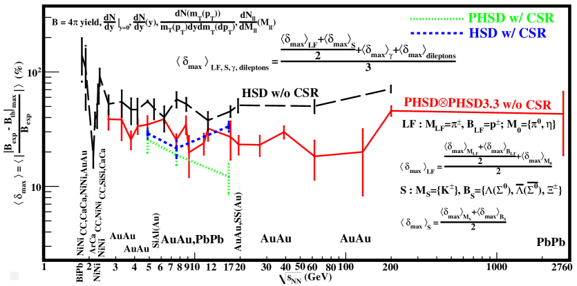
Figure 1: The worst relative criteria of comparison between models and experimental data as a function of the energy of central nucleus-nucleus collisions. The formulas are demonstrating the method described in the text. $LF,S$ are a sets of light flavor and strange hadrons respectively. Models without chiral symmetry restoration are denoted with ”w/o”. The points are connected by the lines to guide the eye.

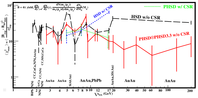
Figure 2: The worst $\chi^{2}$-criteria of comparison between models and experimental data as a function of the energy of central nucleus-nucleus collisions. Models without chiral symmetry restoration are denoted with ”w/o”. The points are connected by the lines to guide the eye.

Taking into account reasonings from [14], [19] and [20], interpretation of Fig. 1 and Fig. 2 is next. The separation of the worst $\chi^{2}$-criteria of PHSD and HSD models already at $\sqrt{s_{NN}}\,=\,2.7$ GeV (they only touch each other by errors) could be caused by ignition of QGP at top SIS energies (the full star at Fig. 3). I remind, that dependence of the worst $\chi^{2}$-criterion from an experimental error is reduced as described above. As partonic degree of freedom uses at most $40\%$ of the collision energy at top SPS energies [19] then it would be possible to say that at top SIS energies this QGP state of matter should occupy small part of a volume of the created fireball (other its largest part of volume consist of hadronic matter). Then the fireball can be regarded as consisting of drop of hot and dense exotic matter with temperature greater than temperature of the fireball’s peripheral hadronic corona. The separation of the worst relative criteria of PHSD and HSD models at $\sqrt{s_{NN}}\,=\,3.5$ GeV could be explained by the transition of QGP phase into Quarkyonic phase of matter - phase trajectory of a system (of a drop of exotic matter) intersect phase boundary (the point 3.5 GeV at Fig. 3). The phase trajectory of hadronic corona stays in the hadronic phase at this energy of collisions (Corona’s trajectory up to the point 3.5 GeV at Fig. 3). The energy pumped up into the fireball during nuclei collision is not enough to support the QGP phase in the drop at $\sqrt{s_{NN}}\,=\,3.5$ GeV because of increased volume of the fireball in comparison with its volume at top SIS energies (the estimation of volume is shown below). The separations of the worst relative criteria at $\sqrt{s_{NN}}\,=\,4.3$ GeV - $5.2$ GeV and the worst $\chi^{2}$-criteria of PHSD and HSD models at $\sqrt{s_{NN}}\,=\,4.6$ GeV - $5.5$ GeV give hint that at energy around $\sqrt{s_{NN}}\,=\,(4.3+4.6)/2\,=\,4.45$ GeV phase trajectory reaches the boundary between Hadronic and Quarkyonic states of matter (the point 4.4 GeV at Fig. 3). That is, the pumped up energy into the fireball at $\sqrt{s_{NN}}\,=\,4.3$ GeV is not enough to support Quarkyonic phase of matter of a drop because of, again, the increased volume of the fireball. The phase trajectory does not intersect this boundary but goes along it (the matter stays in the pre-Quarkyonic phase which is a some kind of confind matter which is different from pure hadronic one [21]) up to point corresponded to energy around $\sqrt{s_{NN}}\,=\,(5.5+5.2)/2\,=\,5.35$ GeV (the point 5.3 GeV at Fig. 3). Subsequent overturn of the worst $\chi^{2}$-criteria of HSD and PHSD relatively to each other and coincidence of the worst relative criteria could be interpreted as returning phase trajectory into the Quarkyonic phase after $\sqrt{s_{NN}}\,=\,5.35$ GeV. That is, the pumped up energy into the fireball is enough to return drop’s matter in the Quarkyonic phase. At point corresponded to around $\sqrt{s_{NN}}\,=\,9.3$ GeV the phase trajectory reaches the critical end point moving on the inside of Quarkyonic phase [20] - I take into account the sharp decreasing of the worst relative and $\chi^{2}$-criteria of PHSD after $8.8$ GeV with their minimums at $\sqrt{s_{NN}}\,=\,9.2$ GeV and divergence of the worst relative criteria for PHSDwCRS and HSDwCRS after $9.2$ GeV and their the worst $\chi^{2}$-criteria after $10$ GeV: $\frac{8.8+9.2+9.2+10}{4}=9.3$ GeV. As PHSD assumes transition to QGP over smooth (2-nd order) crossover, the next similar behaviour of two types of the worst criteria with their intersections at around $\sqrt{s_{NN}}\,=\,12.3$ GeV I interpret as the subsequent moving of phase trajectory, after critical end point, along boundary of transition with a smooth crossover between Quarkyonic and QGP phases up to triple point [20]. After triple point corresponded to around $\sqrt{s_{NN}}\,=\,12.3$ GeV (the intersection is visible there for both types of criteria) phase trajectory of a drop remains in the QGP phase. The phase trajectory of corona’s matter stays in the hadronic phase at all range of considered energies of nuclei collisions. At the Fig. 3, a possible scenario of phase trajectory of a drop at low SIS/BEVALAC energies was shown but other models are needed to figure out that phase trajectory.

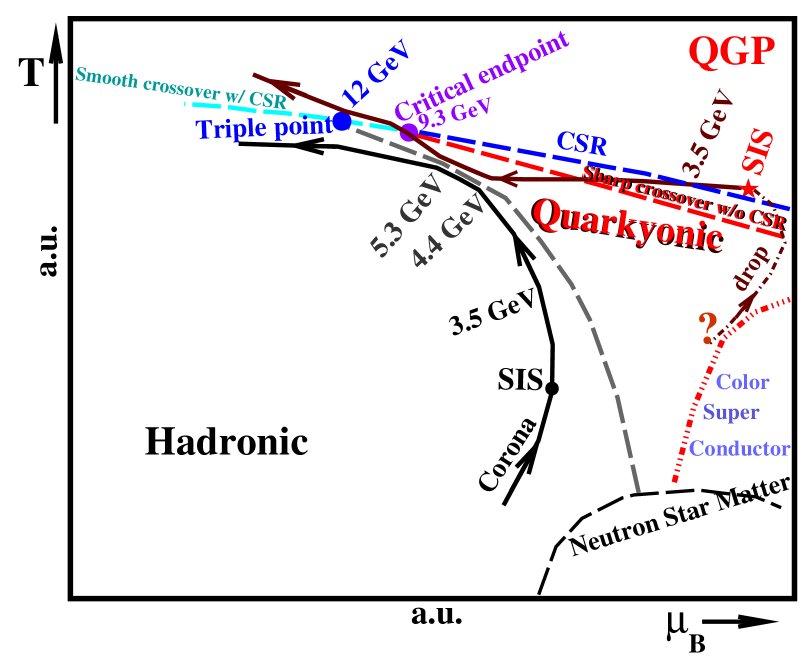
Figure 3: The sketch of the phase diagram of strongly interacting matter and the phase trajectories (with arrows) of a systems created in the central nucleus-nucleus collisions: Corona’s phase trajectory - a phase trajectory of a matter of peripheral outer layer of a fireball; the drop’s phase trajectory (solid with dash-dot line) - a phase trajectory of matter of central part of fireball. Temperature $T$ and baryon chemical potential $\mu_{B}$ are the values averaged over all time of existance and volume occupied by the drop or corona (see text).

Temperature and baryon chemical potential at Fig. 3 are understood by me as values averaged over all time of existence of drop or corona and over their volumes, but not as commonly used a freeze-out values [22]. That is, let the drop (corona) exist during time interval $\Delta_{d(c)}=\tau_{f}-\tau_{0}$, where $\tau_{0}$ is a time of formation of drop (corona) and $\tau_{f}$ is a time of a freezing-out, a disappearing, of drop (corona). The temperature of a drop is higher than corona and it increases toward center of a drop. Moreover, it is a function of time. The averaged volume of a drop (corona) over time interval its existance is $V_{d(c)}=\frac{1}{\Delta_{d(c)}}\int_{\tau_{0}}^{\tau_{f}}V_{d(c)}(t)dt$. Then averaged temperature of a drop (corona) is $T\equiv\langle T\rangle_{d(c)}=\frac{1}{\Delta_{d(c)}\cdot V_{d(c)}}\int_{\tau_{0}}^{\tau_{f}}\int_{v}T_{d(c)}(t,r)dtd^{3}r$, $\langle T\rangle_{d}>\langle T\rangle_{c}$. And I assume that $\langle T\rangle_{d}>\langle T\rangle_{fball}$, where the averaged temperature of whole fireball obtained analogously. The same for baryon chemical potential: $\mu_{B}\equiv\,\langle\mu_{B}\rangle_{d(c)}=\frac{1}{\Delta_{d(c)}\cdot V_{d(c)}}\int_{\tau_{0}}^{\tau_{f}}\int_{v}\mu_{Bd(c)}(t,r)dtd^{3}r$.

Let’s now estimate the radius and volume of a drop (corona) created in central collisions of nuclei. Let experiment measures the yield of particles created during time of fireball’s existence and produced over all volume of fireball $Y^{exp}_{fball}$. Assume that the phase of matter of drop is $A$ and the phase of matter of corona is $B$. Let theory $T_{1}$ describes fireball evolution paying not attention to co-existance of phase $B$ with $A$, assuming only phase’s $A$ existance. Then theory $T_{1}$ predicts yield of particles from phase $A$: $Y^{T_{1}}_{A}$. Let now theory $T_{2}$ describes fireball evolution paying not attention to co-existance of phase $A$ with $B$, assuming only phase’s $B$ existance. Then theory $T_{2}$ predicts yield of particles from phase $B$: $Y^{T_{2}}_{B}$. But experimental value $Y^{exp}_{fball}$ equal to sum of yields of particles from both phases: $Y^{exp}_{fball}=Y_{A}+Y_{B}$ and that summands can not be measured separately by experiment. Suppose that there are such numbers (there are such properties of created matter) $a_{1(2)}$ that $a_{1}=Y^{exp}_{fball}/Y_{A}\approx V_{fball}/V_{d},\,a_{2}=Y^{exp}_{fball}/Y_{B}\approx V_{fball}/V_{c}$, where $V_{d,c,fball}$ are an averaged volumes of drop, corona, fireball over their life time up to freeze-out. Then relative criterion $\delta=(Y^{exp}_{fball}-Y^{T_{1(2)}}_{A(B)})/Y^{exp}_{fball}=1-Y^{T_{1(2)}}_{A(B)}/Y^{exp}_{fball}=1-Y^{T_{1(2)}}_{A(B)}/(a_{1(2)}Y_{A(B)})$. Now let theories $T_{1(2)}$ can be regarded as very good. I.e., although they can strongly deviate from experiment: $Y^{T_{1(2)}}_{A(B)}\neq Y^{exp}_{fball}$, but at least approximately $Y^{T_{1(2)}}_{A(B)}\approx Y_{A(B)}$. Therefore, $\delta\approx 1-1/a_{1(2)}\approx 1-\frac{V_{d(c)}}{V_{fball}}$. Thus, the averaged relative criteria over all type of particles gives possibility to estimate averaged volume of different phases of the fireball. Exactly saying, the averaged relative criterion for yields of all type of particles shows a averaged volume is not occupied by phase considered by used theory. In the [23] I used larger statistics for yields than in this work because did not exlude criteria with large errors, what smeared the picture, but in result Fig.1 of [23] shows not only the agreement theory with experiment, but and relative volume of HG (hadron gas) and QGP phases in the range from AGS to RHIC energies. For example, the averaged volume is not occupied by HG (3FD with hadronic EoS model) in the fireball created in central heavy ion collisions at $\sqrt{s_{NN}}\,=\,63$ GeV is 100$\%$, what means that at this energy QGP phase fills all volume of fireball. At $\sqrt{s_{NN}}\,=\,2.7$ GeV, all 3 versions of used model, HG version and two QGP versions of 3FD (3-Fluid Dynamic), have the averaged relative criteria around 15$\%$. It is logically to assume that not occupied by HG (3FD with hadronic EoS does not assume coexistance of other phase) the averaged volume is 15$\%$: $V_{HG}=85\%$, then $V_{QGP}=100-85=15\%$. If we take radius of fireball created at $\sqrt{s_{NN}}\,=\,2.7$ GeV is 10 fm [24], then radius of drop of QGP is around 5.3 fm. Analogously, the volume of a exotic drop at $\sqrt{s_{NN}}\,=\,3.2$ GeV (Fig.1 of [23]) is around 10$\%$ of whole volume of fireball, therefore the drop’s radius is around 5.1 fm if radius of fireball has been increased up to, for example, 11 fm. That is, small volume of QGP’s drop does not mean its small radius because of cubic dependence between them. I note, that the increase of temperature of drop towards its center and the larger averaged temperature of a drop than chemical freeze-out temperature of fireball were not considered in [24] and in its conclusions. Now, let’s take density of QGP is 0.7 $fm^{-3}$ [24], then averaged distance between partons is 0.55 fm. Taking reasonings from [25] that if germ of new phase, immersed in the other phase, has size (5.1 fm) between the mean interparticle distance (0.55 fm) and the system size (11 fm) then this is a mesoscopic system ”with deconfinement being rather a sharp crossover” (1-st order) [25]. So, at around $\sqrt{s_{NN}}\,=\,3.5$ GeV the preferential transition is a sharp crossover and taking into account reasonings from [26] this sharp crossover transition is split from chiral symmetry restoration transition. Their boundaries meet in critical endpoint at $\sqrt{s_{NN}}\,=\,9.3$ GeV. According to [26], this splitting is a small and chiral symmetry restoration temperature is higher than deconfinement, sharp crossover in our case, temperature.

Two words about calculation of criterion of some function from combination of observables. At Fig. 4, taken from Fig.7 of [14], results of calculations by (7) of $\chi^{2}$-criterion of agreement PHSDwCSR with experimental data for ratios of yields of strange to non-strange hadrons $K^{+}/\pi^{+}$ and $\Lambda/\pi^{-}$ are shown. First summand of (7) is calculated as

$$\Phi_{\chi^{2},T}(\frac{K^{+}}{\pi^{+}})=\frac{((\frac{K^{+}}{\pi^{+}})_{exp}-(\frac{K^{+}}{\pi^{+}})_{T})^{2}}{\sigma^{2}_{exp}}$$ (11)

directly from Fig. 4 for three points: at $\sqrt{s_{NN}}\,=\,4.9,\,7.6,\,17.3$ GeV (only for that energies, article [14] has data for model’s calculation of hadronic yields for next calculations). $T$ is a PHSDwCSR. The second summand of (7) is calculated from data for rapidity distributions taken from Fig.4-6 of [14] for the same three points:

$$\Phi_{\chi^{2},T}(K^{+},\pi^{+})=\frac{1}{2}(\frac{(K^{+}_{exp}-K^{+}_{T})^{2}}{\sigma^{2}_{exp}}+\frac{(\pi^{+}_{exp}-\pi^{+}_{T})^{2}}{\sigma^{2}_{exp}}).$$ (12)

Then final result is:

$$\langle F_{\chi^{2},T}(\frac{K^{+}}{\pi^{+}})\rangle=\frac{1}{3}\sum\frac{1}{2}(\Phi_{\chi^{2},T}(\frac{K^{+}}{\pi^{+}})+\Phi_{\chi^{2},T}(K^{+},\pi^{+})),$$ (13)

where summation runs over that three points and result is shown at left side of Fig. 4. The same procedure was done for $\Lambda/\pi^{-}$ for the same energy points and result is shown at the right side of Fig. 4. For comparison, the results of fitting of calculations by Hadron Resonance Gas Model (HRGM) with the same ratios were taken from [27] and [28] and shown at Fig. 4 also. Though authors of [27] and [28] have proclaimed about the successful description of these ratios by HRGM they do not give information how the model describes numerator and denominator separately with the best set of fitting parameters taken from successful fitting of ratios. Therefore, their statement can be regarded as premature.

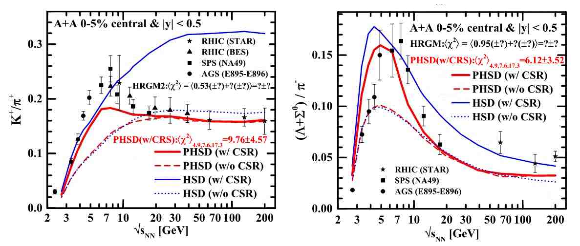
Figure 4: The ratios $K^{+}/\pi^{+}$ (l.h.s.) and $\Lambda/\pi^{−}$ (r.h.s.) at midrapidity from $5\%$ central Au+Au collisions as a function of the energy $\sqrt{s_{NN}}$. The figures were copied from Fig.7 of [14]. Points for HRGM(2) are not shown though they are very close to experimental points in a limits of errors. Calculation of $\langle\chi^{2}\rangle$ was done by (11 - 13).

4 CONCLUSION

Application of the meta-analysis has allowed to separate HSD and PHSD models already at energy $\sqrt{s_{NN}}\,=\,2.7$ GeV of central nucleus-nucleus collisions, though the amount of published data is not enough yet for separation of HSDwCSR and PHSDwCSR models below $\sqrt{s_{NN}}\,=\,6$ GeV. The meta-analysis has figured out the possible position of critical endpoint at around $\sqrt{s_{NN}}\,=\,9.3$ GeV, a triple point at around $\sqrt{s_{NN}}\,=\,12$ GeV and the boundaries of a states of nuclear matter at QCD phase diagram: the transition at $\sqrt{s_{NN}}\,=\,3.5$ GeV corresponds to a split sharp crossover transition and chiral symmetry restoration between QGP and Quarkyonic matter, the boundary of transition with a partial chiral symmetry restoration between Hadronic and Quarkyonic matter was localized between $\sqrt{s_{NN}}\,=\,$4.4 and 5.3 GeV, although it is not being crossed by phase trajectories of drop or corona. The boundary of a smooth crossover transition with chiral symmetry restoration between Quarkyonic matter and QGP was localized between $\sqrt{s_{NN}}\,=\,$9.3 and 12 GeV. The ignition of QGP’s drop happens at top SIS energies.

The calculation of temperatures and baryon chemical potentials of drop and corona parts of fireball is needed what will allow to figure out the curvatures of phase boundaries. Other models are needed to figure out the phase trajectory of a system at low SIS/BEVALAC energies.

References

- [1] Laplace P-S. Théorie Analytique des Probabilités. Oeuvres Complètes 7 (3rd edition). Paris: Courcier, 1820: lxxvii.
- [2] Airy GB. On the Algebraical and Numerical Theory of Errors of Observations and the Combination of Observations. London: Macmillan and Company, 1861.
- [3] V. A. Kizka, V. S. Trubnikov, K. A. Bugaev, D. R. Oliinychenko, arXiv:1504.06483 [hep-ph].
- [4] W. Cassing et al., Proceedings of the 3rd International Conference on New Frontiers in Physics, Kolymbari, Crete, July 28th - Aug. 6th, (2014); arXiv:1408.4313 [nucl-th].
- [5] W. Cassing, E.L. Bratkovskaya, Nucl. Phys. A 831, (2009) 215-242; arXiv:0907.5331 [nucl-th].
- [6] J. Geiss, W. Cassing, C. Greiner, Nucl. Phys. A 644, (1998) 107-138; arXiv:nucl-th/9805012.
- [7] W. Cassing, E. L. Bratkovskaya, Physics Reports 308, (1999) 65-233.
- [8] E. L. Bratkovskaya et al., Proceedings of the International Symposium on ‘Exciting Physics’, Makutsi-Range, South Africa, 13-20 November, 2011; arXiv:1202.4891 [nucl-th].
- [9] E. L. Bratkovskaya et al., 27th Winter Workshop on Nuclear Dynamics (WWND) in Colorado, USA on February 6 - 13, 2011; arXiv:1106.1859 [nucl-th].
- [10] T. Anticic et al. (NA49 Collaboration), Phys. Rev. C 86, (2012) 054903; arXiv:1207.0348 [nucl-exp].
- [11] T. Anticic et al. (NA49 Collaboration), Phys. Rev. C 80, (2009) 034906; arXiv:0906.0469 [nucl-exp].
- [12] E. L. Bratkovskaya et al., Phys. Rev. C 69 (2004) 054907; arXiv:nucl-th/0402026
- [13] H. Weber, E. L. Bratkovskaya, W. Cassing, H. Stoecker, Phys. Rev. C 67 (2003) 014904; arXiv:nucl-th/0209079
- [14] W. Cassing, A. Palmese, P. Moreau, E. L. Bratkovskaya, arXiv:1510.04120v1 [nucl-th].
- [15] V. P. Konchakovski, W. Cassing, V. D. Toneev, J. Phys. G: Nucl. Part. Phys. 42, (2015) 055106; arXiv:1411.5534 [nucl-th].
- [16] O. Linnyk et al., Phys. Rev. C 92, (2015) 054914; arXiv:1504.05699 [nucl-th].
- [17] Pierre Moreau et al., Proceedings of the 15th International Conference on Strangeness in Quark Matter (SQM2015), 6-11 July 2015, JINR, Dubna, Russia; arXiv:1509.04455 [nucl-th].
- [18] E. L. Bratkovskaya et al., Proceedings of the 28th Winter Workshop on Nuclear Dynamics, Dorado del Mar, Puerto Rico, April 7-14, 2012; arXiv:1207.3198 [nucl-th].
- [19] O. Linnyk, E. L. Bratkovskaya, W. Cassing, J. Phys. G: Nucl. Part. Phys. 37, (2010) 094039; arXiv:1001.2914v1 [nucl-th].
- [20] A. Andronic et al., Nucl. Phys. A 837, (2010) 65-86; arXiv:0911.4806v3 [hep-ph].
- [21] Larry McLerran, Robert D. Pisarski, Nucl. Phys. A796, (2007) 83-100; arXiv:0706.2191v3 [hep-ph].
- [22] A. Bazavov et al., Phys. Rev. D 93, (2016) 014512; arXiv:1509.05786v2 [hep-lat].
- [23] V. A. Kizka, arXiv:1508.03196 [nucl-th].
- [24] D. A. Fogaca, S. M. Sanches Jr., R. Fariello, F. S. Navarra, arXiv:1601.04596v1 [hep-ph].
- [25] V.I. Yukalov, E.P. Yukalova, Proc. Sci. (ISHEPP) (2012) 046; arXiv:1301.6910 [hep-ph].
- [26] C. A. Dominguez, M. Loewe, Y. Zhang, Phys. Rev. D 86, (2012) 034030; arXiv:1205.3361v3 [hep-ph].
- [27] V. V. Sagun, UJP 59, 8, (2014) 755-763; arXiv:1408.6110 [hep-ph].
- [28] K. A. Bugaev et al., arXiv:1412.6571 [hep-ph].